Uncertain Production Scheduling Based on Fuzzy Theory Considering Utility and Production Rate


1
School of Information and Control Engineering, Liaoning Shihua University, Fushun 113001, China
2
National Experimental Teaching Demonstration Center of Petrochemical Process Control, Liaoning Shihua University, Fushun 113001, China
3
State Key Laboratory of Industrial Control Technology, Institute of Cyber-Systems and Control, Zhejiang University, Hangzhou 310027, China
4
Zhejiang Supcon Software Co., Ltd., Hangzhou 310053, China
5
School of Innovation and Entrepreneurship, Shenzhen Polytechnic, Shenzhen 518055, China
*
Author to whom correspondence should be addressed.
Information 2017, 8(4), 158; https://doi.org/10.3390/info8040158
Submission received: 26 October 2017
/
Revised: 25 November 2017
/
Accepted: 27 November 2017
/
Published: 18 December 2017
(This article belongs to the Special Issue Smart Sensing, Information Security and Control of Industrial Cyber-Physical Systems)
Abstract
:Handling uncertainty in an appropriate manner during the real operation of a cyber-physical system (CPS) is critical. Uncertain production scheduling as a part of CPS uncertainty issues should attract more attention. In this paper, a Mixed Integer Nonlinear Programming (MINLP) uncertain model for batch process is formulated based on a unit-specific event-based continuous-time modeling method. Utility uncertainty and uncertain relationship between production rate and utility supply are described by fuzzy theory. The uncertain scheduling model is converted into deterministic model by mathematical method. Through one numerical example, the accuracy and practicability of the proposed model is proved. Fuzzy scheduling model can supply valuable decision options for enterprise managers to make decision more accurate and practical. The impact and selection of some key parameters of fuzzy scheduling model are elaborated.
1. Introduction
A cyber-physical system (CPS) was identified as a key research area by the US National Science Foundation (NSF) and was listed as the number one research priority by the US President’s Council of Advisors on Science and Technology [1]. In recent years, CPS is attracting much attention and is being considered as an emerging technology. It has wide potential applications in defense [2,3], transportation [4], industrial automation [5], energy [6,7], health care [1,8] and agriculture [9,10], etc. Cyber-physical systems (CPS) can be viewed as a new generation of systems with integrated control, communication and computational capabilities [1]. It combines computation and communication capabilities with the physical world [11].
Uncertainty is intrinsic in most technical systems, including CPS. CPS generally functions in an inherently complex and unpredictable physical environment. A major difficulty with CPS is that it must be designed and operated in the presence of uncertainty [12]. Therefore, handling uncertainty in an appropriate manner during the real operation of CPS is critical. In CPS, physical components are inserted by sensors and actuators. Sensors have the abilities of self-calibration, dynamic parameter setting, Ethernet-based communication and self-adaptation [13]. So CPS has enough capability to detect uncertainties in itself or from external environment.
For a manufacturing enterprise, the real operation of CPS is just the execution of production scheduling. So the uncertainty problem of production scheduling is a part of the CPS uncertainty issue. Uncertainties in manufacturing are various, which include demand uncertainty, processing time uncertainty, utility uncertainty, due date uncertainty, equipment failure and the absence of employee. For the uncertain scheduling problem of batch process, some research results have been obtained. Guillen, et al. [14] proposed a multistage stochastic optimization model to address the scheduling of supply chains with embedded multipurpose batch chemical plants under demand uncertainty. Zhu, et al. [15] proposed a robust optimization approach for the short-term scheduling of batch plants under demand uncertainty where the uncertain parameters can be described by a normal distribution function. Ierapetritou [16] developed a strategy to quantify scheduling robustness in the face of uncertainty, to increase scheduling flexibility, and to improve system performance when unexpected events occur during scheduling execution. Xu, et al. [17] established a scheduling mathematical model for multi-product batch processes under finite intermediate storage policy with uncertain processing time based on fuzzy programming theory.
Nowadays, most studies mainly deal with uncertainties of demand and processing time in production scheduling. Research on utility uncertainty is rare, and the supply amount of utility is assumed to be constant. In fact, utility disturbance is an important uncertain factor to the production process. In the production process, utilities such as steam, cooling water and electricity, are supplied to areas or product lines to support the normal operation of equipment. Sometimes, these utilities are shared by different areas. However, the utility supply is affected seriously by the energy system, and the energy system is also disturbed by many uncertainty factors. So, utility disturbances usually occur, which will affect the normal running of machines, make the scheduling decision infeasible, even leads to the shutdown of the product line [18,19,20]. Consequently, dealing with utility uncertainty well in production scheduling is vital to enterprise competitiveness. Moreover, the production rate is closely related to the utility supply. The relationship between them is roughly assumed to be linear in most studies, which is unable to reflect the actual production situation. So building the uncertain relationship between the production rate and the utility supply is another key point for production scheduling.
For the above two uncertainties, it is time-consuming and material-consuming to establish a mechanism model [21]. Existing methods to describe uncertainty include chance constraint programming, fuzzy theory and scenario trees [22,23]. Chance constraint programming needs a large amount of historical data to analyze the distribution function of uncertainty [24]. The scenario trees method adds many constraints, enables a large programming model scale, and has a computation time too long to meet requirements [25]. If the historical data of uncertainty is insufficient or difficult to acquire, then fuzzy theory is an effective means.
In this paper, a MINLP uncertain scheduling model for batch process is formulated based on unit-specific event-based continuous-time (USEBCT) modeling method. Fuzzy method is utilized to describe the uncertainty of utility supply. For the uncertain relationship between the production rate and the utility supply, firstly establish the linear function in deterministic scheduling model, and then use fuzzy method to represent the coefficient of linear function. The uncertain scheduling model is converted into deterministic model by mathematical method. Through one numerical example, the accuracy and practicability of the proposed model are proved.
This paper is organized as follows: Section 2 describes the problem definition of short scheduling for batch process. Section 3 formulates the deterministic scheduling model. Section 4 details the fuzzy scheduling model and the defuzzification method. A numerical example and roles of proposed model are given in Section 5. Conclusions are presented in Section 6.
2. Problem State
The short-term scheduling problem for batch processes is stated as follows. Given (i) the production recipe (i.e., the amount of the materials required for the production of each product); (ii) the available units, their capacity limits and utility; (iii) the available storage capacity for each of the materials; and (iv) the time horizon under consideration, then the objective is to determine (i) the optimal sequence of tasks taking place in each unit; (ii) the amount of material being processed at each time in each unit; and (iii) the processing time of each task in each unit.
3. Deterministic Scheduling Model Based on USEBCT Modeling Method
The USEBCT model is proposed by Ierapetritou and Floudas [31]. The USEBCT model permits event to happen at any moment in the scheduling horizon. The duration time of every event is varying. The scale of mathematical programming is smaller, and the computation time is shorter, so compared with discrete-time model, USEBCT model is more actual and accurate in describing the production situation.
3.1. Basic Concepts of USEBCT Model
- (1)
- Event: time measurement, each event has one start time and finish time;
- (2)
- State: raw materials, intermediates and final products;
- (3)
- Task: action of producing or consuming one state;
- (4)
- Unit: machines in which the task can be performed.
3.2. Deterministic Scheduling Model
The proposed deterministic scheduling model is formulated based on the model framework proposed by Vooradi and Shaik (V&S model) [26]. For the reason of computation time, is set to be zero. Moreover, material balances, duration constraints, tightening constraints and utility constraints are modified according to the requirements of modeling.
(1) Allocation constraints
In every unit, at the most one task can be active at each event as given by constraint (1), in which is binary variable. If task is active at event , , else .
(2) Capacity constraints
Constraint (2) limits the size of one batch. If task is active at event , then the decision variable of processed material is forced in the range of the minimum and maximum batch sizes. Otherwise, is forced to be zero.
(3) Material balances
When ,
When ,
Constraints (3) and (4) are material balances of raw materials, intermediates and products at initial event. Constraints (5)–(7) are material balances of the above three states at the later events. If n is equal to 1, the amount of states (raw material or intermediate) at event n is equal to the initial value, and decreased by any amounts consumed at event n, as given by constraint (3). The amount of final product at event n is calculated as initial value, as given by constraint (4).
If , the amount of a state at current event is adjusted by any amounts produced by tasks that ends at the previous event and adjusted by any amounts consumed by the tasks that starts at the current event, as given by constraint (5) to constraint (7).
(4) Duration constraints
In order to formulate the relationship between consumption of utility and production rate, the variable is introduced to represent the production rate of task at event . The finish time of task at event is equal to the start time plus duration time of the task, which is calculated by .
In constraint (9), production rate is formulated by the summery of minimum production rate, which maintains the equipment running, and linear function of consumption of utility. The parameter is assumed as a constant number in deterministic model. However the relationship between consumption of utility and production rate is not linear simply. In fuzzy model, the parameter is defined as a fuzzy number to describe the uncertain relationship between consumption of utility and production rate as given by constraint (25).
(5) Sequencing constraints
① Same task in the same unit
In constraint (10), the start time of task at event should be greater than or equal to the finish time of the same task at event .
② Different tasks in the same unit
The constraint (11) is written for two different tasks performed in the same unit at event and , respectively. If task is active at event , the start time of task must be greater than or equal to the finish time of previous task .
③ Different tasks in different units
According to the production recipe, for different tasks that produce or consume the same state, the start time of the consuming task at the next event is enforced to be later than the finish time of the producing task at the current event as given by constraint (12). Otherwise, the constraint is relaxed and the two times are not related.
(6) Tightening constraints
The sum of the durations of all tasks suitable in each unit should be less than the scheduling horizon as given by constraint (13).
(7) Utility constraints
The consumption of utility is a linear function of amount of processed material, which is given by constraint (14). The consumption of utility is limited by the total supply amount of utility. Constraint (15) expresses that the consumption of utility at event should not be greater than the maximum supply. The maximum supply amount of utility is another uncertain parameter and assumed as a constant number in deterministic model. But the supply amount of utility is affected seriously by energy system, and the energy system is also disturbed by lots of uncertain factors. So, utility disturbances usually occur. In fuzzy model, the parameter is defined as a fuzzy number to describe the uncertain utility supply as given by constraint (26).
Constraint (16) is similar to that for same task in the same unit written for each utility. The start time of consuming utility at event should not be earlier than that at event .
To account for the utility consumption over different tasks, constraints (17) and (18) enforce the start time of all suitable tasks that consume the same utility to be equal to , if the task is active at event .
If , constraints (17) and (18) can be rewritten by and , which is equivalent to . If , constraints (17) and (18) are relaxed.
In constraint (19), the finish times of all suitable tasks that consume a utility at previous event are enforced to occur before, if the task is active. Otherwise, constraint (19) is relaxed.
(8) Storage constraints
Infinite storage and dedicated finite intermediate storage policies are considered in this work. Constraint (20) expresses the limit of storage capacity. For handling dedicated finite intermediate storage case, constraint (21) along with constraint (12) is used to avoid real time storage violations without the need for considering storage as a separate task.
If constraints (12) and (21) are not relaxed, constraint (22) is workable. In constraint (22), the finish time of producing task at event should be greater than or equal to the start time of consuming task at the same event, and less than or equal to the start time of consuming task at event .
(9) Bounds on variables
Constraint (23) initials the consumption time of utility at the first event, and limits all the start and finish times of tasks to be within the scheduling horizon.
(10) Objective function
The objective function is the maximization of profit, and the total amount of the final products produced by the end of last event is calculated by constraint (24).
4. Fuzzy Scheduling Model and Defuzzification
4.1. Uncertainty Description
Coefficient and maximum supply amount of utility are fuzzy numbers, as given by constraints (25) and (26). The two fuzzy numbers are described by triangular possibility distributions. This description of fuzzy numbers has been extensively used in literatures due to their various advantages (e.g., Lai and Hwang, 1992 [32], 1993 [33], Liang, 2006 [34] and 2008 [35]). The simplicity in required data acquisition and simplicity in related fuzzy computations are the most important advantages [36,37,38]. These advantages are our main motivation in using the triangular fuzzy numbers for modeling the imprecise data in our problem. Figure 1 presents the triangular possibility distribution of fuzzy number , where , and are the most pessimistic value, the most possible value, and the most optimistic value. The triangular possibility distribution of is defined as Equation (27).
The universe U of fuzzy number is defined as Equation (28) according to Basyigit and Ulu [39], where is the minimum value in statistical data of fuzzy number, is the maximum value in statistical data of fuzzy number. and are defined as Equation (29) and (30) according to the experience of engineering. is the value of which the frequency of occurrence is the most in statistical data of fuzzy number.
Typically, the three prominent values, i.e., the most pessimistic, the most possible, and the most optimistic values for fuzzy numbers are estimated by decision maker [32,37,40]. In this paper, the three prominent values are defined according to determining method of universe [39] and the experience of engineering. The most pessimistic value is equal to the left boundary of universe. The most possible value is equal to . The most optimistic value is equal to the right boundary of universe. These relationships are given by Equations (31) to (33).
The deterministic scheduling model is replaced by the following fuzzy scheduling model:
Objective function: (24)
Constraints: (1)–(8), (10)–(14), (16)–(23)
(25), deterministic constraint (9) is replaced by fuzzy constraint (25)
(26), deterministic constraint (15) is replaced by fuzzy constraint (26).
4.2. Defuzzification of Fuzzy Scheduling Model
Defuzzification is a process whereby the fuzzy scheduling model is converted into a deterministic scheduling model. Constraint (25) can be converted into inequality constraints. All the fuzzy numbers are on one side of inequality constraints, so fuzzy numbers ranking problem is not involved. We apply the well-known weighted average method. This approach seems to be the simplest and most reliable defuzzification method in converting the fuzzy constraints into their deterministic ones [35,37,38,41]. In this regard, we also need to determine a minimal acceptable possibility level , which denotes the minimum acceptable possibility level of occurrence for the corresponding imprecise/fuzzy data. So, the equivalent deterministic constraints can be represented as follows:
where , and , and represent the weights of the most pessimistic, the most possible and the most optimistic value of the related fuzzy numbers, respectively. In practice, the suitable values for these weights as well as are usually determined subjectively by the experience and knowledge of the decision maker. Based on the most likely value concept proposed by Lai and Hwang [32] and considering several relevant works [42,43], we set these parameters to: = 1/6, = 4/6, = 1/6 in numerical experiments. , , , , , are boundary points of -cut fuzzy set. Take as example, boundary points calculated by (37) to (39). The relationships among them are illustrated in Figure 2.
Equivalent deterministic model through defuzzification is reformulated as follows:
Objective function: (24)
Constraints: (1)–(8), (10)–(14), (16)–(23) and (34)–(36).
5. Case Study
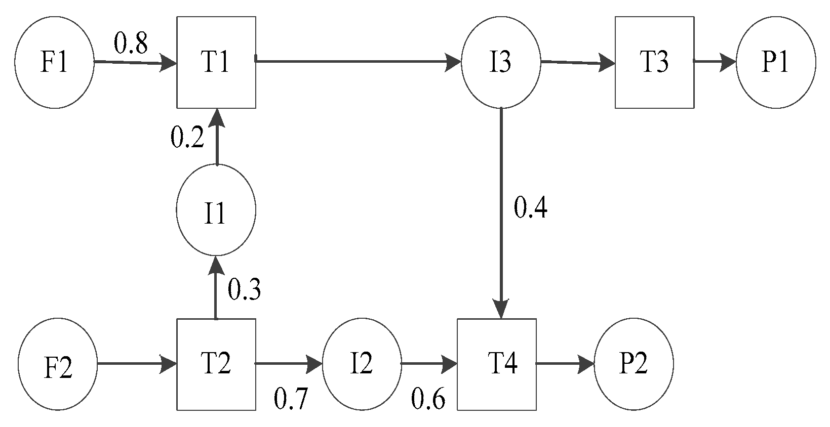
Numerical example is introduced firstly by Maravelias and Grossmann [44] and has been studied in several studies [31,45]. As shown in Figure 3, this example involves four tasks in three units processing seven states. The corresponding data is given in Table 1 and Table 2. There are two types of reactors available for the process (type I and II) with different number of corresponding units available: two reactors (RI1 and RI2) of type I, while one reactor (RII) of type II. Reactions R1 and R2 require type I reactor, while reactions R3 and R4 require type II reactor. Furthermore, reactions R1 and R3 require heat, provided by steam (HS) produced in limited amounts in the plant, while reactions R2 and R4 are exothermic and require cooling water (CW), also available in limited amounts. Due to safety reasons and temperature restrictions, the heat integration of the process is not possible.
The minimum batch-size for all tasks is the half of maximum capacities of units. Finite storage policy for intermediates and unlimited storage policy for the raw materials, final products, are applied. Numerical example is solved using Lingo 11.0 (Lindo Systems, Chicago, IL, USA) with a 2.20 GHz computer. Scheduling horizon is seven hours, and event number is set to 5. A better optimization solution cannot be found by larger event numbers. The data of fuzzy numbers are given in Table 3 and Table 4. Three prominent values (most pessimistic value, most possible value, and most optimistic value) of fuzzy numbers are in parentheses.
In order to demonstrate the advantages of proposed fuzzy mode, we input a set of actual data into the deterministic model. The results based on the actual data are viewed as a criterion for comparing the accuracy of deterministic model and fuzzy model. Actual data of fuzzy number and are given in Table 3 and Table 4.
.
Results based on actual data, of deterministic model and fuzzy model are compared in Table 5. In this numerical example, = 1/6, = 4/6, = 1/6. The objective function (maximization of profit) based on actual data is 5448$. The corresponding completion time is 11.20 h, which is the sum of processing time of three machine units (RI1, RI2 and RII).
The objective function of deterministic model is 5400$.The completion time of deterministic model is 12.30 h. For fuzzy model, the objective function ranges from 5426.25$ to 5410.50$, correspondingly, varies from 0.5 to 0.8. Completion time also varies depending on different . In order to compare the optimization results better, deviations of deterministic and fuzzy models as well as average values of deviations for fuzzy model are given in Table 6. Based on data in Table 5, taking results of actual data as criterion, the deviations of deterministic model and fuzzy model are calculated by formula , where is the measured data and is truth-value. Results of deterministic and fuzzy models are used as measured data. Results based on actual data are used as truth-value.
In the deterministic scheduling model, some uncertain parameters like and are assumed as constant numbers. In the fuzzy scheduling model, these uncertain parameters are defined as fuzzy numbers, which considers the uncertainties in scheduling problem. Actual data of these uncertain parameters are fluctuant, but not constant. Results based on actual data are optimized through the collected data from actual operating condition, which can reflect the practical situation of production line. So the results closer to that based on actual data should be more practical. For accuracy, in this paper, we view the results based on actual data as the truth-value to evaluate the accuracy of deterministic model and fuzzy model, because it is fairer than just comparing the results of deterministic model and fuzzy model. Consequently, the results closer to that based on actual data should be more accurate. As shown in Table 6, the average values of deviations in terms of objective function and completion time about fuzzy model are 0.545% and 5.09%, which are all smaller than that of deterministic model. It means that the results of fuzzy model are closer to results based on actual data. So the proposed fuzzy model is more practical and accurate than deterministic model.
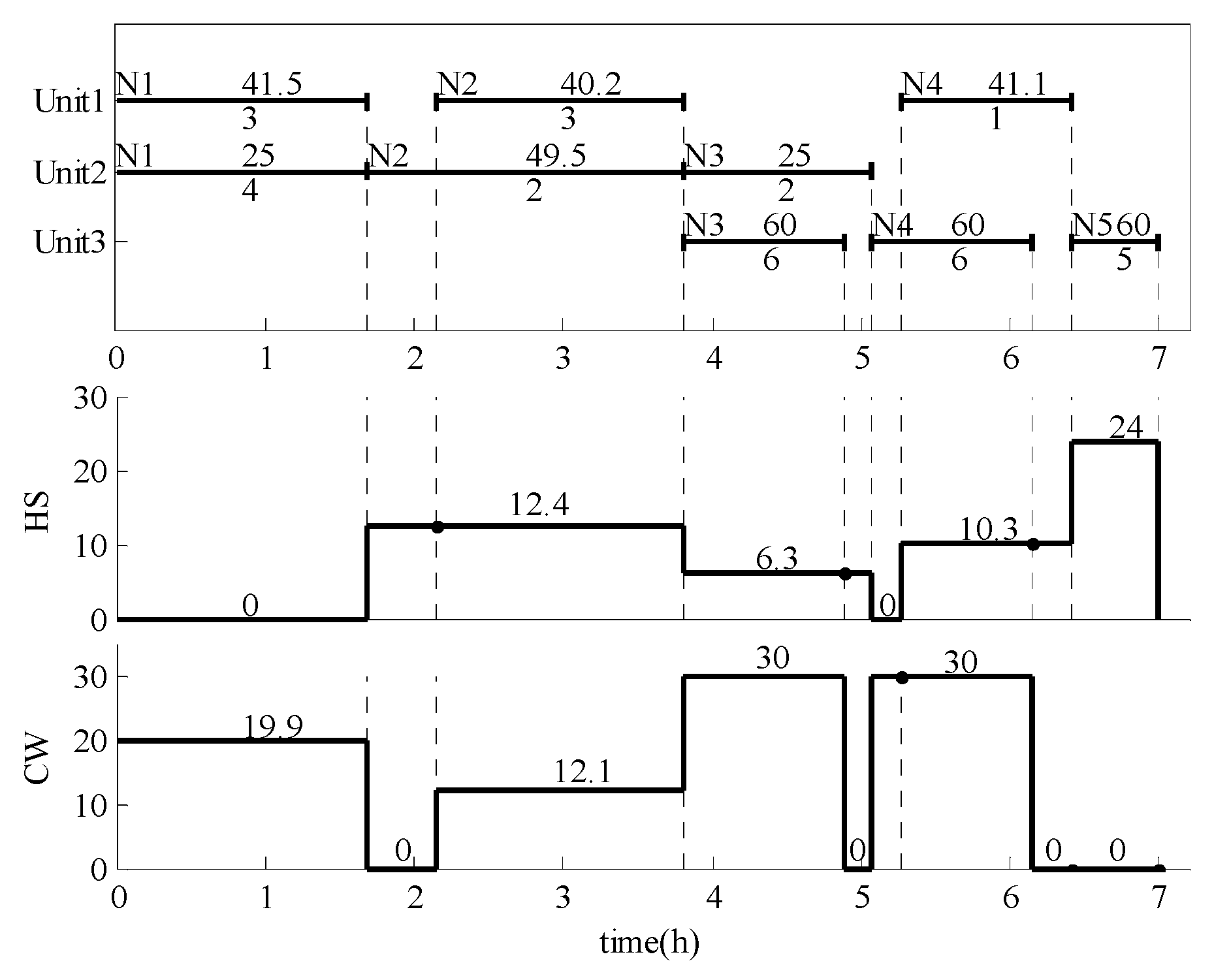
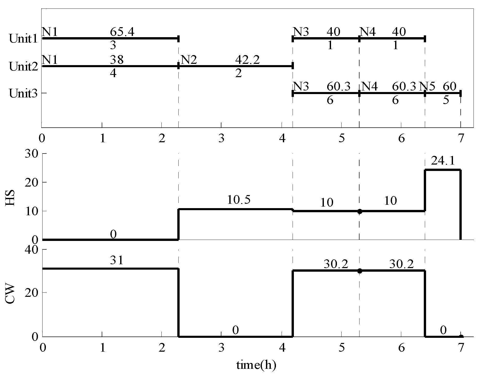
Fuzzy scheduling model can supply valuable decision options for enterprise managers to make decision more accurate and practical. Decision maker can adjust the acceptable possibility level , according to risks taken by enterprises, and then obtain more accurate and practical scheduling results. The smaller decider chooses, the higher risks are taken by enterprise, but the profit will be greater and the scheduling results will be more far away from that of deterministic model. In contrast, the larger decider chooses, the lower risks are taken by enterprise, but the profit will be less and the scheduling results will be closer to that of deterministic model. In addition to objective function and completion time, Gantt charts for deterministic model and fuzzy model are illustrated in Figure 4 and Figure 5.
It is noteworthy that the membership function of fuzzy number is vital for the quality of fuzzy scheduling results. If membership function is not symmetry and tends to the superior side, the objective function of fuzzy model will be better than that of deterministic model, and vice versa. So one precise membership function analyzed by historical data, is an important support for the accuracy of optimization results of fuzzy scheduling model. Some parameters, for example acceptable possibility level and weights , and , also have important impact on optimization result of fuzzy model. However these parameters only affect optimization result on quantitative value but not on the quality as membership function. With the increasing of acceptable possibility level , the optimization result gets close to that of deterministic model. That is because the greater the acceptable possibility level is, the more the fuzzy number is close to the most possible value. The selection of depends on decision maker. If decision maker doesn’t want to take too much risk, the acceptable possibility level should be greater, and vice versa. Weights , and , represent the inclination extent to most pessimistic value, the most possible value, and the most optimistic value in membership function. The three weights are usually selected by experience.
6. Conclusions
In this paper, a MINLP uncertain model for batch process is formulated based on the unit-specific event-based continuous-time modeling method. Utility uncertainty and uncertain relationship between production rate and utility supply are described by fuzzy theory. The uncertain scheduling model is converted into deterministic model by mathematical method. The accuracy and practicability of the proposed model is proved through one numerical example. Fuzzy scheduling model can supply valuable decision options for enterprise managers to make decision more accurate and practical. The impact and selection of some key parameters of fuzzy scheduling model are elaborated.
Acknowledgments
This work is supported by Key Project of Natural Science Foundation Program of Liaoning Province (No. 20170520319), supported by Open Research Project of the State Key Laboratory of Industrial Control Technology, Zhejiang University, China (No. ICT170286) and supported by Talent Scientific Research Fund of LSHU (No. 2016XJJ-101).
Author Contributions
Yue Wang conceived, formulated and verified the scheduling model. Yue Wang, Xin Jin, Lei Xie and Shan Lu analyzed the results, discussed the manuscript and corrected the manuscript. Yanhui Zhang contributed on experience about fuzzy number. All authors have read and approved the final manuscript.
Conflicts of Interest
The authors declare no conflict of interest.
Nomenclature
| Upper layer: | |
| Indices | |
| task | |
| unit | |
| event | |
| state | |
| utility | |
| Sets | |
| tasks | |
| tasks which can be performed in unit j | |
| tasks which produce state | |
| tasks which consume state | |
| tasks which consume utility | |
| units | |
| units which are suitable for performing task | |
| total events postulated in the scheduling horizon | |
| states | |
| states that are raw materials | |
| states that are final products | |
| states that are intermediates | |
| utilities | |
| utilities that are required by task | |
| intermediate states with dedicated finite intermediate storage | |
| Parameters | |
| minimum batch size of task | |
| maximum batch size of task | |
| initial amount available for state | |
| maximum storage capacity for state | |
| proportion of state consumed by task | |
| proportion of state produced by task | |
| coefficient between production rate and consumption of utility consumed by task | |
| minimum production rate of task | |
| price of state | |
| large positive number in big-M constraints | |
| short-term scheduling horizon | |
| coefficient between consumption of utility and amount of material consumed/processed by task at event | |
| maximum availability of utility for task | |
| limit on the maximum number of events over which a task is allowed to continue | |
| Binary variables | |
| binary variable for task active at event | |
| Positive variables | |
| amount of material processed by task at event | |
| production rate of task at event | |
| excess amount of state that needs to be stored at event | |
| start time of a task at event | |
| end time of a task at event | |
| consumption of utility by task at event | |
| start time at which there is a change in the consumption of utility at event |
References
- Wang, J.; Abid, H.; Lee, S.; Shu, L.; Xia, F. A Secured Health Care Application Architecture for Cyber-Physical Systems. J. Control Eng. Appl. Inform. 2011, 13, 101–108. [Google Scholar]
- Satchidanandan, B.; Kumar, P.R. Dynamic Watermarking: Active Defense of Networked Cyber–Physical Systems. Proc. IEEE 2016, 105, 219–240. [Google Scholar] [CrossRef]
- Niu, H.; Jagannathan, S. Optimal Defense and Control for Cyber-Physical Systems. In Proceedings of the 2015 IEEE Symposium Series on Computational Intelligence, Cape Town, South Africa, 7–10 December 2015; pp. 634–639. [Google Scholar]
- Moller, D.P.F.; Vakilzadian, H. Cyber-physical systems in smart transportation. In Proceedings of the IEEE International Conference on Electro Information Technology, Grand Forks, ND, USA, 19–21 May 2016; pp. 776–781. [Google Scholar]
- Thramboulidis, K. A cyber-physical system-based approach for industrial automation systems. Comput. Ind. 2015, 72, 92–102. [Google Scholar] [CrossRef]
- Al Faruque, M.A.; Ahourai, F. A model-based design of Cyber-Physical Energy Systems. In Proceedings of the 19th Asia and South Pacific, Design Automation Conference, Singapore, 20–23 January 2014; pp. 97–104. [Google Scholar]
- Ilic, M.D.; Xie, L.; Khan, U.A. Modeling future cyber-physical energy systems. In Proceedings of the 2008 IEEE Power and Energy Society General Meeting—Conversion and Delivery of Electrical Energy in the Century, Pittsburgh, PA, USA, 20–24 July 2008; pp. 1–9. [Google Scholar]
- Costanzo, A.; Faro, A.; Giordano, D.; Pino, C. Mobile cyber physical systems for health care: Functions, ambient ontology and e-diagnostics. In Proceedings of the IEEE Consumer Communications & Networking Conference, Las Vegas, NV, USA, 9–12 January 2016; pp. 972–975. [Google Scholar]
- Mehdipour, F. Smart Field Monitoring: An Application of Cyber-Physical Systems in Agriculture (Work in Progress). In Proceedings of the IIAI 3rd International Conference on Advanced Applied Informatics, Kitakyushu, Japan, 31 August–4 September 2014; pp. 181–184. [Google Scholar]
- Rad, C.R.; Olteanu, G.; Takacs, I.A.; Olteanu, G. Smart Monitoring of Potato Crop: A Cyber-Physical System Architecture Model in the Field of Precision Agriculture. Agric. Agric. Sci. Procedia 2015, 6, 73–79. [Google Scholar] [CrossRef]
- Haque, S.A.; Aziz, S.M.; Rahman, M. Review of Cyber-Physical System in Healthcare. Int. J. Distrib. Sens. Netw. 2014, 10, 20. [Google Scholar] [CrossRef]
- Zhang, M.; Selic, B.; Ali, S.; Yue, T.; Okariz, O.; Norgren, R. Understanding Uncertainty in Cyber-Physical Systems: A Conceptual Model. In Modelling Foundations and Applications; Springer International Publishing: Cham, The Switzerland, 2016. [Google Scholar]
- Berger, C.; Hees, A.; Braunreuther, S.; Reinhart, G. Characterization of Cyber-Physical Sensor Systems. Procedia CIRP 2016, 41, 638–643. [Google Scholar] [CrossRef]
- Guillén, G.; Mele, F.D.; Antonio Espuña, A.; Puigjaner, L. Addressing the Design of Chemical Supply Chains under Demand Uncertainty. Comput. Aided Chem. Eng. 2006, 21, 1095–1100. [Google Scholar]
- Zhu, J.; Gu, X.; Gu, W. Robust optimization approach for short-term scheduling of batch plants under demand uncertainty. Kybernetes 2011, 40, 860–870. [Google Scholar] [CrossRef]
- And, J.P.V.; Ierapetritou, M.G. Robust Short-Term Scheduling of Multiproduct Batch Plants under Demand Uncertainty. Ind. Eng. Chem. Res. 2001, 40, 4543–4554. [Google Scholar]
- Xu, Z.H.; Gu, X.S.; Jiao, B. Scheduling of Uncertain Multi-product Batch Processes Under Finite Intermediate Storage Policy. IFAC Proc. Vol. 2008, 41, 14864–14869. [Google Scholar]
- Lindholm, A.; Johnsson, C. Plant-wide utility disturbance management in the process industry. Comput. Chem. Eng. 2013, 49, 146–157. [Google Scholar] [CrossRef]
- Lindholm, A.; Giselsson, P. Minimization of economical losses due to utility disturbances in the process industry. J. Process Control 2013, 23, 767–777. [Google Scholar] [CrossRef]
- Lindholm, A.; Johnsson, C.; Quttineh, N.-H.; Lidestam, H.; Henningsson, M.; Wikner, J.; Tang, O.; Nytzen, N.-P.; Forsman, K. Hierarchical Scheduling and Utility Disturbance Management in the Process Industry. IFAC Proc. Vol. 2013, 46, 140–145. [Google Scholar] [CrossRef]
- Wang, K.; Choi, S.H.; Lu, H. A hybrid estimation of distribution algorithm for simulation-based scheduling in a stochastic permutation flowshop. Comput. Ind. Eng. 2015, 90, 186–196. [Google Scholar] [CrossRef]
- Aytug, H.; Lawley, M.A.; Mckay, K.; Mohan, S.; Uzsoy, R. Executing production schedules in the face of uncertainties: A review and some future directions. Eur. J. Oper. Res. 2005, 161, 86–110. [Google Scholar] [CrossRef]
- Sabuncuoglu, I.; Goren, S. Hedging production schedules against uncertainty in manufacturing environment with a review of robustness and stability research. Int. J. Comput. Integr. Manuf. 2009, 22, 138–157. [Google Scholar] [CrossRef]
- Mou, D.; Chang, X. An Uncertain Programming for the Integrated Planning of Production and Transportation. Math. Probl. Eng. 2014, 2014, 135–142. [Google Scholar] [CrossRef]
- Li, Y.P.; Huang, G.H.; Chen, X. Multistage scenario-based interval-stochastic programming for planning water resources allocation. Stoch. Environ. Res. Risk Assess. 2009, 23, 781–792. [Google Scholar] [CrossRef]
- Vooradi, R.; Shaik, M.A. Improved three-index unit-specific event-based model for short-term scheduling of batch plants. Comput. Chem. Eng. 2012, 43, 148–172. [Google Scholar] [CrossRef]
- Munawar, A.S.; Christodoulos, A.F. Improved Unit-Specific Event-Based Continuous-Time Model for Short-Term Scheduling of Continuous Processes: Rigorous Treatment of Storage Requirements. Ind. Eng. Chem. Res. 2007, 46, 1764–1779. [Google Scholar]
- Shaik, M.A.; Floudas, C.A. Novel Unified Modeling Approach for Short-Term Scheduling. Ind. Eng. Chem. Res. 2009, 48, 2947–2964. [Google Scholar] [CrossRef]
- Shaik, M.A.; Floudas, C.A. Unit-specific event-based continuous-time approach for short-term scheduling of batch plants using RTN framework. Comput. Chem. Eng. 2008, 32, 260–274. [Google Scholar] [CrossRef]
- Castro, P.; Barbosa-Póvoa, A.P.F.D.; Matos, H. An Improved RTN Continuous-Time Formulation for the Short-term Scheduling of Multipurpose Batch Plants. Ind. Eng. Chem. Res. 2001, 40, 5040–5041. [Google Scholar] [CrossRef]
- Ierapetritou, M.G.; Floudas, C.A. Effective continuous-time formulation for short-term scheduling. 1. Multipurpose batch processes. Ind. Eng. Chem. Res. 1998, 37, 4341–4359. [Google Scholar] [CrossRef]
- Lai, Y.J.; Hwang, C.L. A new approach to some possibilistic linear programming problems. Fuzzy Sets Syst. 1992, 49, 121–133. [Google Scholar] [CrossRef]
- Lai, Y.J.; Hwang, C.L. Possibilistic linear programming for managing interest rate risk. Fuzzy Sets Syst. 1993, 54, 135–146. [Google Scholar] [CrossRef]
- Liang, T.F. Distribution planning decisions using interactive fuzzy multi-objective linear programming. Fuzzy Sets Syst. 2006, 157, 1303–1316. [Google Scholar] [CrossRef]
- Liang, T.F. Integrating production-transportation planning decision with fuzzy multiple goals in supply chains. Int. J. Prod. Res. 2008, 46, 1477–1494. [Google Scholar] [CrossRef]
- Torabi, S.A.; Hassini, E. An interactive possibilistic programming approach for multiple objective supply chain master planning. Fuzzy Sets Syst. 2008, 159, 193–214. [Google Scholar] [CrossRef]
- Torabi, S.A.; Ebadian, M.; Tanha, R. Fuzzy hierarchical production planning (with a case study). Fuzzy Sets Syst. 2010, 161, 1511–1529. [Google Scholar] [CrossRef]
- Torabi, S.A. Multi-site production planning integrating procurement and distribution plans in multi-echelon supply chains: An interactive fuzzy goal programming approach. Int. J. Prod. Res. 2009, 47, 5475–5499. [Google Scholar] [CrossRef]
- Basyigit, A.I.; Ulu, C.; Guzelkaya, M. A New Fuzzy Time Series Model Using Triangular and Trapezoidal Membership Functions. In Proceedings of the International Work-Conference on Time Series, Granada, Spain, 25–27 June 2014. [Google Scholar]
- Noori-Darvish, S.; Mahdavi, I.; Mahdavi-Amiri, N. A bi-objective possibilistic programming model for open shop scheduling problems with sequence-dependent setup times, fuzzy processing times, and fuzzy due dates. Appl. Soft Comput. J. 2012, 12, 1399–1416. [Google Scholar] [CrossRef]
- Wang, R.C.; Liang, T.F. Applying possibilistic linear programming to aggregate production planning. Int. J. Prod. Econ. 2005, 98, 328–341. [Google Scholar] [CrossRef]
- Garciasabater, J.P. Capacity and material requirement planning modelling by comparing deterministic and fuzzy models. Int. J. Prod. Res. 2008, 46, 5589–5606. [Google Scholar]
- Christou, I.T.; Lycopoulou, A.G.L.D. Hierarchical production planning for multi-product lines in the beverage industry. Prod. Plan. Control 2007, 18, 367–376. [Google Scholar] [CrossRef]
- Maravelias, C.T.; Grossmann, I.E. A New General Continuous-Time State Task Network Formulation for Short-Term Scheduling of Multipurpose Batch Plants. Ind. Eng. Chem. Res. 2003, 42, 3056–3074. [Google Scholar] [CrossRef]
- Wang, Y.; Su, H.; Shao, H.; Xie, L. Unit-Specific Event-Based and Slot-Based Hybrid Model Framework with Hierarchical Structure for Short-Term Scheduling. Math. Probl. Eng. 2015, 2015, 1–15. [Google Scholar] [CrossRef]
Figure 1.
Triangular possibility distribution of fuzzy number.
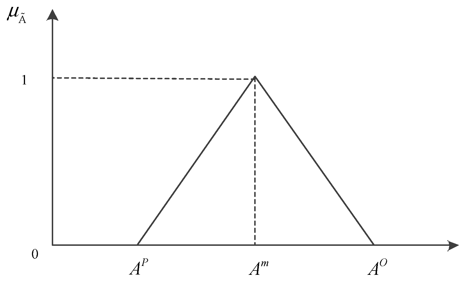
Figure 2.
Triangular possibility distribution of fuzzy number.
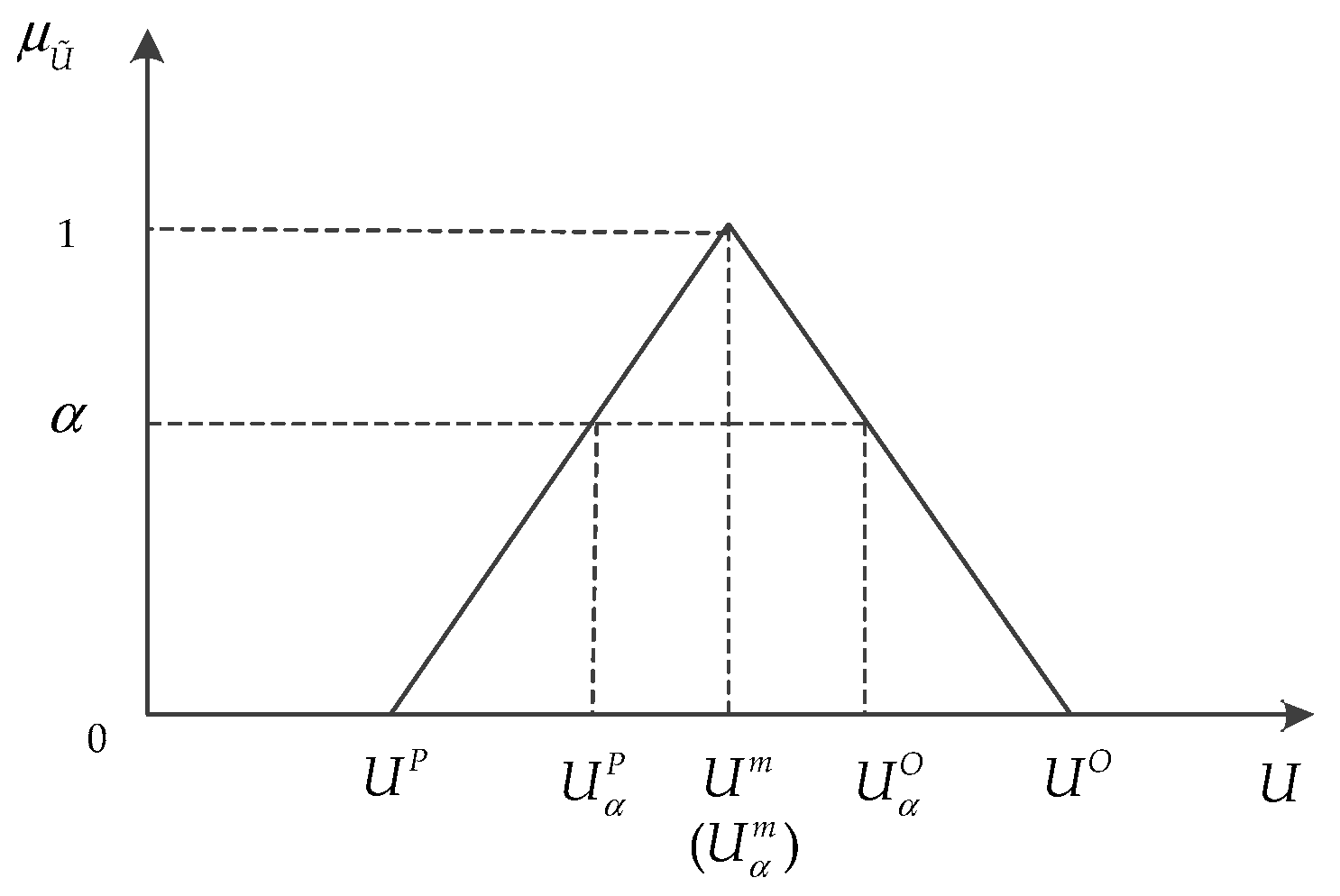
Figure 3.
State-task network representation.

Figure 4.
Gantt chart for the deterministic model.

Figure 5.
Gantt chart for the fuzzy model.


Table 1.
Data of production capability and coefficients of utility consumption.
| Task 1 (R1) | Task 2 (R2) | Task 3 (R3) | Task 4 (R4) | |||
|---|---|---|---|---|---|---|
| RI1 | 40 | 80 | 0.25 | 0.3 | - | - |
| RI2 | 25 | 50 | 0.25 | 0.3 | - | - |
| RII | 40 | 80 | - | - | 0.2 | 0.5 |
, in kg, in kg per kg of batch.
Table 2.
Data related States.
| F1 | F2 | I1 | I2 | I3 | P1 | P2 | |
|---|---|---|---|---|---|---|---|
| STsmax | 1000 | 1000 | 200 | 100 | 500 | 1000 | 1000 |
| STs0 | 400 | 400 | 0 | 0 | 0 | 0 | 0 |
| Prices | 0 | 0 | 0 | 0 | 0 | 30 | 40 |
STsmax (kg), STs0 (kg) in kg, Prices in $/kg.
Table 3.
Data of fuzzy number
| Task 1 | Task 2 | Task 3 | Task 4 | ||||
|---|---|---|---|---|---|---|---|
| RI1 | RI2 | RI1 | RI2 | RII | RII | ||
| three prominent values | (0.8 1 1.3) | (0.4 0.6 0.7) | (0.55 0.6 0.62) | (0.4 0.5 0.6) | (1.9 2 2.2) | (0.9 1 1.2) | |
| actual data | event 1 | 0.92 | 0.65 | 0.60 | 0.45 | 1.95 | 0.95 |
| event 2 | 0.90 | 0.60 | 0.61 | 0.50 | 2.10 | 1.00 | |
| event 3 | 0.98 | 0.62 | 0.60 | 0.50 | 2.00 | 0.98 | |
| event 4 | 1.00 | 0.58 | 0.59 | 0.51 | 1.98 | 1.10 | |
| event 5 | 1.15 | 0.50 | 0.58 | 0.55 | 2.00 | 1.00 | |
Table 4.
Data of fuzzy number .
| Task 1 | Task 2 | Task 3 | Task 4 | ||||
|---|---|---|---|---|---|---|---|
| RI1 | RI2 | RI1 | RI2 | RII | RII | ||
| three prominent values | (23 24 25) | (20 24 27) | (27 30 35) | (28 30 31) | (22 24 27) | (29 30 33) | |
| actual data | event 1 | 23.5 | 25.5 | 32.5 | 30.0 | 25.4 | 29.7 |
| event 2 | 24.0 | 23.0 | 31.2 | 30.5 | 23.6 | 31.5 | |
| event 3 | 23.8 | 24.0 | 28.5 | 30.0 | 24.0 | 29.6 | |
| event 4 | 24.5 | 22.0 | 30.0 | 29.4 | 24.0 | 30.0 | |
| event 5 | 24.0 | 24.7 | 29.6 | 29.0 | 23.0 | 30.8 | |
Table 5.
Optimization results of deterministic model and fuzzy model.
| Results Based on Actual Data | Deterministic Model | Fuzzy Model | ||||
|---|---|---|---|---|---|---|
| Objective Function ($) | Completion Time (h) | Objective Function ($) | Completion Time (h) | Objective Function ($) | Completion Time (h) | |
| 5448 | 11.20 | 5400 | 12.30 | 0.5 | 5426.25 | 11.42 |
| 0.6 | 5421.00 | 12.10 | ||||
| 0.7 | 5415.75 | 12.19 | ||||
| 0.8 | 5410.50 | 11.37 | ||||
Table 6.
Deviation analysis.
| Deterministic Model | Fuzzy Model | |||
|---|---|---|---|---|
| Objective Function ($) | Completion Time (h) | Objective Function ($) | Completion Time (h) | |
| 0.88% | 9.82% | 0.5 | 0.40% | 1.96% |
| 0.6 | 0.50% | 8.04% | ||
| 0.7 | 0.59% | 8.84% | ||
| 0.8 | 0.69% | 1.52% | ||
| average value | 0.545% | 5.09% | ||
© 2017 by the authors. Licensee MDPI, Basel, Switzerland. This article is an open access article distributed under the terms and conditions of the Creative Commons Attribution (CC BY) license (http://creativecommons.org/licenses/by/4.0/).
Share and Cite
MDPI and ACS Style
Wang, Y.; Jin, X.; Xie, L.; Zhang, Y.; Lu, S. Uncertain Production Scheduling Based on Fuzzy Theory Considering Utility and Production Rate. Information 2017, 8, 158. https://doi.org/10.3390/info8040158
AMA Style
Wang Y, Jin X, Xie L, Zhang Y, Lu S. Uncertain Production Scheduling Based on Fuzzy Theory Considering Utility and Production Rate. Information. 2017; 8(4):158. https://doi.org/10.3390/info8040158
Chicago/Turabian StyleWang, Yue, Xin Jin, Lei Xie, Yanhui Zhang, and Shan Lu. 2017. "Uncertain Production Scheduling Based on Fuzzy Theory Considering Utility and Production Rate" Information 8, no. 4: 158. https://doi.org/10.3390/info8040158
Note that from the first issue of 2016, this journal uses article numbers instead of page numbers. See further details here.