Hybridizing Adaptive Biogeography-Based Optimization with Differential Evolution for Multi-Objective Optimization Problems


1
College of Information Science&Technology, Hainan University, No. 58 Renmin Avenue, Haikou 570228, China
2
State Key Laboratory of Marine Resource Utilization in the South China Sea, Hainan University, No. 58 Renmin Avenue, Haikou 570228, China
*
Author to whom correspondence should be addressed.
Information 2017, 8(3), 83; https://doi.org/10.3390/info8030083
Submission received: 22 May 2017
/
Revised: 5 July 2017
/
Accepted: 11 July 2017
/
Published: 14 July 2017
Abstract
:In order to improve the performance of optimization, we apply a hybridization of adaptive biogeography-based optimization (BBO) algorithm and differential evolution (DE) to multi-objective optimization problems (MOPs). A model of multi-objective evolutionary algorithms (MOEAs) is established, in which the habitat suitability index (HSI) is redefined, based on the Pareto dominance relation, and density information among the habitat individuals. Then, we design a new algorithm, in which the modification probability and mutation probability are changed, according to the relation between the cost of fitness function of randomly selected habitats of last generation, and average cost of fitness function of all habitats of last generation. The mutation operators based on DE algorithm, are modified, and the migration operators based on number of iterations, are improved to achieve better convergence performance. Numerical experiments on different ZDT and DTLZ benchmark functions are performed, and the results demonstrate that the proposed MABBO algorithm has better performance on the convergence and the distribution properties comparing to the other MOEAs, and can solve more complex multi-objective optimization problems efficiently.
1. Introduction
Biogeography-based optimization (BBO) algorithm (Simon, 2008) [1] is proposed based on the mechanism for biological species migrating from one place to another. As a population-based stochastic algorithm, BBO algorithm generates the next generation population by simulating the migration of the biological species. Two main operators in BBO algorithm are the migration and mutation. Migration operation is based on the emigration rate and immigration rate of each individual in the population. Mutation operation is performed by mutation probability. BBO algorithm has some advantages due to information sharing in the migration process, especially for single-objective optimization problems (SOPs) [2,3,4,5]. BBO algorithm can also be used to solve multi-objective benchmark problems [6,7].
The aim of this paper is to propose and study multi-objective biogeography-based optimization (MBBO) algorithms, including modified migration operator, modified mutation operator, and adaptive modification and mutation probability. This paper proposes a new multi-objective biogeography-based optimization algorithm called MABBO, and then presents a comparative study on multi-objective benchmark functions.
The motivation for proposing MABBO in this research is threefold. First, we have observed that the definition of habitat suitability index (HSI) should take into account the dominant relation, and the distribution of solutions [6]. Second, there are several good results based on the hybridization of BBO with differential evolution (DE) [8,9]. Last, blend combination operators have been widely and successfully used in other population-based optimization algorithms [10].
The original contributions of this paper include the following. Firstly, the model of applying BBO for multi-objective evolutionary algorithm was established, in which the habitat suitability index is redefined, based on the Pareto dominance relation and density information among the habitat individuals. Motivated by the work in [11,12], we hybridize adaptive BBO with DE to design a new algorithm for multi-objective optimization problems. In this algorithm, the mutation operator based on DE algorithm was modified, and the migration operator based on the number of iterations was re-designed to achieve better performance. Furthermore, the modification probability and mutation probability are adaptively changed, according to the relation between the cost of fitness function of randomly selected habitats of last generation, and average cost of fitness function of all habitats of last generation. Experiments performed on ZDT and DTLZ benchmark functions show that the obtained Pareto solution set can approximate to the Pareto optimal front, and has good diversity and uniform distribution. The results also demonstrate that the proposed MABBO algorithm has better performance on the convergence and the distribution.
The paper is organized as follows. Section 2 describes the related work about BBO algorithm. The basic theories of multi-objective optimization are presented in Section 3.The MABBO algorithm procedure for multi-objective optimization problems are proposed in Section 4. Section 5 shows the simulation and experiment results. Finally, a brief conclusion is illustrated in Section 6.
2. Literature Review
Evolutionary computation is an optimization method based on the principles of biological evolution. It maintains a set of entities, which represent possible solutions, and applies some functions that are inspired by biological evolution processes, such as reproduction, migration, mutation, or selection. These solutions compete to prevail over time; only the best solutions will pass to the next generation so that the population evolves. The biogeography-based optimization algorithm based on the mathematical models of biogeography, is a new nature-inspired computation technique to find the optimal solution to the problem. The solution process is analogous to the migration of the species in nature. The BBO algorithm operates on a population of individuals called habitats (or islands). Each habitat represents a possible solution to the problem in hand. The fitness of each habitat is determined by its HSI, which is a metric that determines the goodness of a candidate solution, and each habitat feature is called a suitability index variable (SIV) [2]. A better quality solution is analogous to an island with a high HSI, and an inferior solution is like an island with a low HSI. High HSI solutions are more likely to share their features with other solutions, and low HSI solutions are more likely to accept shared features from other solutions. The sharing of features between solutions is represented as immigration and emigration between the islands [10].
At present, BBO algorithm has had great progress regarding theoretical analysis, algorithm improvement, and application fields. In the theoretical analysis aspect, there is mainly probability analysis and migration model analysis. Probability analysis of approximate values for the expected number of generations before the population’s best solution improves, and the expected amount of improvement, are presented in [11]. These expected values are functions of the population size. In [12], a generalized sinusoidal migration model curve is proposed, and sinusoidal migration models have been shown to provide the best performance so far.
Improvement of the BBO algorithm is mainly based on migration operators and mutation operators, such as with BBO/DE [13,14,15], blended migration operator [16], perturbing biogeography based optimization (PBBO) [17], incorporating opposition-based learning into BBO (OBBO) [18], hybrid quantum with biogeography based optimization (QBBO) [19], and so on. BBO/DE is a hybrid of differential evolution with biogeography-based optimization. The main operator of BBO/DE is the hybrid migration operator, which hybridizes the DE operator with the migration operator of BBO, in an attempt to incorporate diversity, and to overcome stagnation at local optima. Our algorithm incorporates DE into the mutation procedure. PBBO indicates a new migration operation based sinusoidal migration model, which is a generalization of the standard BBO migration operator, and the Gaussian mutation operator is integrated into PBBO, to enhance its exploration ability, and to improve the diversity of population. OBBO improves BBO’s convergence rate as a diversity mechanism. QBBO is proposed by evolving multiple quantum probability models (QPMs). In QBBO, each QPM used to constitute an area in decision space represents a habitat; the whole populations of QPMs evolve as an ecosystem with multiple habitat interaction. The Gaussian mutation operator and Cauchy mutation operator are integrated into real code BBO [20]. In order to enhance the performance of BBO, we modify the mutation operator, and the mutation operator of BBO, in the paper. DE is incorporated into the mutation procedure for multi-objective optimization problems. Motivated by the work in [16], the migration operator is modified based on number of iterations.
Over the past few years, BBO algorithms have wide applications in a variety of fields, such as economic load dispatch problems [21], optimal power flow problems [22], beam pattern design of circular antenna arrays [23], abnormal breast detection via combination of particle swarm optimization and biogeography-based optimization [24], image processing [25], traveling salesman problems [26,27], trajectory planning of robots [28], discrete variables function optimization [29], optimal power flow placement in wireless sensor networks [30], parameter estimation [31,32], permutation flow shop scheduling problems [33], and so on. BBO has demonstrated good performance in various benchmark functions and real-world optimization problems.
Since many real-world optimization problems can be modeled using multiple conflicting objectives, multi-objective optimization has tremendous practical importance. Especially in recent years, the multi-objective optimization based on an evolutionary algorithm has achieved many successful applications [34,35,36,37]. For example, multi-objective genetic algorithms are used in congestion management in deregulated power systems [34]; the multi-objective reactive power price clearing (RPPC) problem was solved using strength pareto evolutionary algorithm (SPEA) and the multi-objective particle swarm optimization (MOPSO) [35]; and multi-objective strength pareto evolutionary algorithm 2+ has been employed to solve congestion management problems [36]. An efficient multi-objective optimization algorithm using the differential evolution (DE) algorithm is proposed to solve multi-objective optimal power flow (MO-OPF) problems [37]. BBO has also been modified to solve multi-objective optimization problems (MOPs) [38,39,40,41,42,43,44,45], such as, multi-objective biogeography-based optimization based on predator-prey approach [38], indoor wireless heterogeneous networks planning [39], automated warehouse scheduling [40], and community detection in social networks with node attributes [41]. Work in the literature [42] is focused on numerical comparisons of migration models for multi-objective biogeography-based optimization. In [43], a novel dynamic non-dominated sorting multi-objective biogeography-based optimization (Dy-NSBBO) is proposed to solve constrained dynamic multi-objective optimization problems. Multi objective non-convex economic dispatch problems are solved by ramp rate biogeography based optimization [44]. Water wave optimization (WWO) and biogeography-based optimization are selected to solve the problem of the integrated civilian–military emergency supplies pre-positioning [45]. Multi-objective biogeography-based optimization has also demonstrated good performance in real-world optimization problems.
3. Multi-Objective Optimization
In principle, multi-objective optimization is different from single-objective optimization. In single-objective optimization, one attempts to obtain the best solution, which is usually the global minimum or the global maximum, depending on the optimization problem. In the case of multiple objectives, there may not be only one solution which is the best (global minimum or maximum), with respect to all objectives. Pareto-optimal solutions are those solutions (from the set of feasible solutions) that cannot be improved in any objective without causing degradation of at least one other objective. If an obtained solution is improved so that at least one objective improves and the other objectives do not decline, then the newly found solution dominates the original solution. The goal of Pareto-optimization is to find the set of solutions that are not dominated by any other solution, which are called non-dominated solutions. The set of these solutions is called the Pareto Front (PF). Without the loss of generality, we consider the minimization MOPs, which can be denoted as follows [6]:
where is called a decision vector with n decision variables, D is an n-dimensional decision space, is an objective vector with M objects, and Z is an m-dimensional objective space. A function mapped from decision space to objective space is defined by , p equality constraint conditions are defined by , and q non-equality constraint conditions are defined by . The several important definitions related to the Pareto domination are given as follows.
Definition 1 (Pareto Domination).
Let , and a decision vector is said to dominate strictly a decision vector , and is denoted by , if and only if
Definition 2 (non-dominated solution).
Let be an arbitrary decision vector, is a subset of solutions, the decision vector is called non-dominated solution with respect to S, if and only if there is no vector in S which dominates a; formally
Definition 3 (Pareto optimal).
The decision vector is called Pareto-optimal with respect to D, if and only if
Definition 4 (Pareto optimal solution).
is called Pareto optimal solution if is non-dominated with respect to all solutions in D. All the Pareto optimal solutions is called Pareto set (PS).
Definition 5 (Pareto front).
The image of all non-dominated solutions is called the Pareto front.
4. MABBO Algorithm
In order to apply BBO algorithm to multi-objective optimization problems, according to the evolutionary mechanism of BBO, the model which applies to BBO for multi-objective evolutionary algorithm is established, in which the habitat suitability index, based on the Pareto dominance relation and density information among the habitat individuals, is redefined. Meanwhile, BBO algorithm has a good exploitation for global optimization [3], however, it is slow in exploring of the search space. On the other hand, DE is good at exploring the search space and locating the region of global minimum. Based on these considerations, in order to balance the exploration and the exploitation of BBO, in this work, we propose a hybrid BBO approach, called MABBO, which combines the exploitation of BBO with the exploration of DE effectively. A new migration operator, based on number of iterations, is also proposed, to improve performance.
4.1. Migrationoperator for MOPs
In BBO, there are two main operators: migration and mutation. The modified migration operator is a generalization of the standard BBO migration operator. The idea is inspired by the blended migration operator [16], and the coefficient of solution Hi is a constant. In our algorithm, as the number of iterations increases, solution Hi is much more fitting than solution Hj. Therefore, solution Hi is more affected by the solution itself. The core idea of the modified migration operator is based on two considerations. On the one hand, blend combination operators have been widely and successfully used in other population-based optimization algorithms. On the other hand, good solutions will be less likely to be degraded due to migration; poor solutions can still accept a lot of new features from good solutions. The migration operator based on number of iterations is designed to accelerate the speed of convergence of the non-dominated solutions. Modified migration is defined as
where is immigrating island, is emigrating island, is the jth dimension of the ith solution, and t is number of iterations, and is maximum number of iterations. Equation (6) means that the features of solution are changed by solutions and . In other words, a new solution after migration is comprised of two components: the migration of the feature from itself, and another solution. At first, a new solution is more affected by another better solution. It accelerates the convergence characteristics of the algorithm. Along with growth of the generation, a new solution is more affected by itself as a solution. The modified migration operator is described as follows:
| Algorithm 1 Migration for MOPs (MigrationDo(H, )) |
| For i = 1 to NP // NP is the size of population If rand < Use to probabilistically decide whether to immigrate to If then For Select the emigrating island with probability If then For j = 1 to Nd // Nd is the dimension size End for End if End for End if End if End for |
4.2. Mutation Operator for MOPs
In BBO, if a solution is selected for mutation, it is replaced by a randomly generated new solution set. This random mutation affects the exploration ability of BBO algorithm. The hybridization of BBO with DE has achieved many good results [13,14,15]. However, they incorporate DE into the migration procedure for single-objective optimization problems. Our algorithm incorporates DE into the mutation procedure. The algorithm adjusts near the optimal solutions so that it can find the non-dominated solutions. In MABBO, modification of mutation operator by integrating with DE produces new feasible solutions. A mutated individual () is generated according to the following equation:
where is selected for mutation, is themutation scaling factor, usually its value is set as 0.5, is randomly selected two solutions, and is the best solution in this generation. In MABBO, this mutation scheme tends to increase the diversity among the population. It acts as a fine tuning unit and helps to achieve a global optimal solution. Modified mutation operator is described as follows:
| Algorithm 2 Mutation for MOPs (Mutation Do(H, )) |
| For i = 1 to NP // NP is the size of population Select mutating habitat with probability If is selected, then For j = 1 to Nd // Nd is the dimension size End for End if End for |
4.3. Adaptive BBO for MOPs
There are modification probability and mutation probability factors in BBO algorithm. Modification probability is denoted as and mutation probability is denoted as . The two factors which range from 0 to 1 are defined by users. When a generated random number is less than modification probability, the program executes the migration operator; when a generated random number is less than the mutation probability, the program executes the mutation operator. In original BBO, modification probability and mutation probability are user-defined parameters. The settings of the parameters are very relevant to the experience of the user, and they are unfavorable for the selection of migration individuals. In order to choose better migration individuals, these parameters are related to the fitness function, and they are adjusted dynamically with the fitness function.
In adaptive BBO algorithm, modification probability and mutation probability are modified according to the relation between the cost of fitness function of randomly selected habitats of last generation, and average cost of fitness function of all habitats last generation. In other words, if the cost of fitness function is equal or greater than average cost, modification probability and mutation probability are modified by Equations (8) and (9), respectively. Otherwise, modification probability and mutation probability are taken as constant k2 and k4, respectively. In Equations (8) and (9), constant factors k1, k2, k3, and k4, which range from 0 to 1, are defined by users. Usually k1 = 0.4, k2 = 0.95, k3 = 0.1, and k4 = 0.25.
4.4. The Redefinition of the Fitness Function
Because multi-objective optimization problems are different from single-objective optimization problems, they balance their objective functions by a set of trade-off solutions, namely Pareto non-dominated solutions set, and the original rule of HSI is no longer applicable to the MABBO algorithm. In the literature [7], the habitat suitability index is only defined based on the Pareto dominance relation. However, it’s not enough to consider Pareto dominance relation; the distribution of these solutions is also important. If the dominant relation and distribution of set of solutions are considered at the same time, the definition of the habitat suitability index will be more reasonable. So the habitat suitability index is redefined based on the Pareto dominance relation and density information among the habitats. For any individual in the habitat population , its rule of HSI is defined by Equation (10) as follows.
In Equation (10), are habitats which contain n-dimensional variables. The operator is the cardinality of the set. Where is the distance between the habitat and the habitat in the objective space, e is integer value of the square root of the sum of population number NP and elitism number . According to Equation (10), the HSI of habitat is determined by its fitness function , which is the sum of and the sum of the percentage of the number of dominated habitats in the total population. In which the number of dominated habitats means the total of the number of any other habitats whom every individual who dominates can dominate in the population. Therefore, the lower the dominated degree of habitat is, the smaller the value of is, and the better HSI of is. The dominated degree of the habitat is 0, and means that is a non-dominated habitat.
4.5. Main Procedureof Improved MABBO for MOPs
By incorporating the above-mentioned migration operator and mutation operator into BBO, and modification probability and mutation probability are modified in term of the relation between the cost of fitness function of randomly selected habitat last generation and average cost of fitness function of all habitats last generation. Meanwhile, the fitness function is redefined according to Pareto dominance relation and distribution information. The MABBO approach is developed and shown in Algorithm 3. MABBO algorithm is able to exploit the population information with the migration operator and to explore the new search space with the mutation operator of DE. This feature overcomes the lack of exploration of the original BBO algorithm. Our proposed MABBO approach is described as follows.
| Algorithm 3 The main procedure of MABBO for MOPs |
|
5. Simulation and Analysis
5.1. Metrics to Assess Performance
Performance metrics play an important role to return a scalar quantity, which reflects the quality of the scrutinized solution set. For MOPs, the quality of solutions can be defined in a variety of ways, for example, the uniformity of solutions, the dominance relationship between solution sets, the closeness to the Pareto optimal front, etc. There are some metrics that can be used to measure the quality of Pareto fronts [42]. The following metrics are used in this paper: generalized distance (GD), spacing (SP), coverage rate (CR), error rate (ER) and convergence index γ.
5.1.1. Generational Distance (GD)
The concept of generational distance was introduced by Van Veldhuizen and Lamont [46]. It evaluates a convergence of solutions set. It is a way to calculate the distance between and . is the approximate Pareto front acquired by MOEAs, while is the true Pareto front. GD is shown in (11).
where is the number of solutions in , is the minimum value of all Euclidean distance between each solution in and each of solutions in . It is clear that a value of GD = 0 indicates that . is the number of solutions in . M is the number of objective dimension, is the function value of the kth objective of the ith solution in , , and are respectively, the jth value, the maximum value, and the minimum value of the kth objective function in . The smaller the GD is, the closer the solution set in is to the Pareto front, and the better the convergence of the algorithm is.
5.1.2. Spacing Metric (SP)
The metric spacing (SP) is used to evaluate the spread of solutions in . Since the “beginning” and “end” of are known, an appropriate metric judges how the solutions distribute. Spacing was proposed by Schoott in [47], which estimates the diversity of solutions. The metric is shown in (12).
where is the number of non-dominated solutions, is Euclidian distance between two consecutive solutions in , and is the average of all . The smaller the SP value, the better the diversity of the population, and the better the distribution of the Pareto solution set. SP = 0 means that all the solutions of the Pareto front are equally distributed.
5.1.3. Coverage Rate (CR)
Coverage rate shown in (13) was proposed by Zitzler et al. [48]. The function C maps the ordered pair (A, B) to the interval [0, 1]:
where A and B are two sets of non-dominated solutions. The value C(A,B) = 1 means that all solutions in B are dominated by or equal to solutions in A. On the other hand, C(A,B) = 0 means that no solutions in B are weakly dominated by A. It should be noted that both C(A,B) and C(B,A) have to be evaluated, since C(A,B) is not always equal to 1−C(B,A).
5.1.4. Error Rate (ER)
ER is used to describe the percentage of solutions that do not belong to the true Pareto front in the non-dominated solutions generated by the algorithm. It is shown in (14).
where n is the number of non-dominated solutions generated by the algorithm. If the solution i belongs to the Pareto optimal solution set, , otherwise . The smaller the ER value is, the higher the proportion of the non-dominated solutions that belong to the Pareto optimal solution set. ER = 0 indicates that all the non-dominated solutions are located on the front of the true Pareto front.
5.1.5. Convergence Index (γ)
If the Pareto optimal solutions set for multi-objective optimization problems is known, some points are evenly taken in the Pareto optimal front for the MOPs (e.g., 500 points), and the minimum value for distance between each solution is obtained by the algorithm and these points is calculated, and the average value of all these minimum values is the convergence index γ. The smaller the convergence index γ is, the better the degree of approximation to the Pareto optimal solution set. When the obtained solution is the same as the point obtained from the Pareto optimal front, γ = 0.
5.2. SimulationComparison and Discussion
In this section, we investigate the performance of MABBO described above on multi-objective benchmark functions having two and three objectives. The results obtained are compared to the Pareto-optimal front of the test problems. We also compare our approach with the results obtained by five other MOEAs (NSGA-II [49], RM-MEDA [50], MOTLBO [51], HMOEA [52] and BBMO [53]); 2-objective and 3-objective test problems [54] were run with different variable numbers. Moreover, in our experiments, under the same conditions, the algorithm runs independently 30 times, and when the evaluation function is called 10,000 times every time, the algorithm terminates running. Due to the limit of the length of the article, we only use the following parameters for the DTLZ7 test problem: DE mutation scheme is DE/rand/1/bin, population size is 100, number of variables in each population is 22, habitat modification probability is 0.75, mutation probability is 0.05, elitism parameter is 10, scaling factor c1 is 0.5, k1 factor is 0.4, k2 factor is 0.95, k3 factor is 0.1, k4 factor is 0.25, generation count is 100, and in every generation, times of loop of the evaluation function is 10. Other test problems have similar parameters to DTLZ7. These parameters that are different from DTLZ7 have number of variables in each population, mutation probability, and modification probability etc.; all parameters used by test problems are presented in Table 1.
5.2.1. MABBO Self Performance Comparison
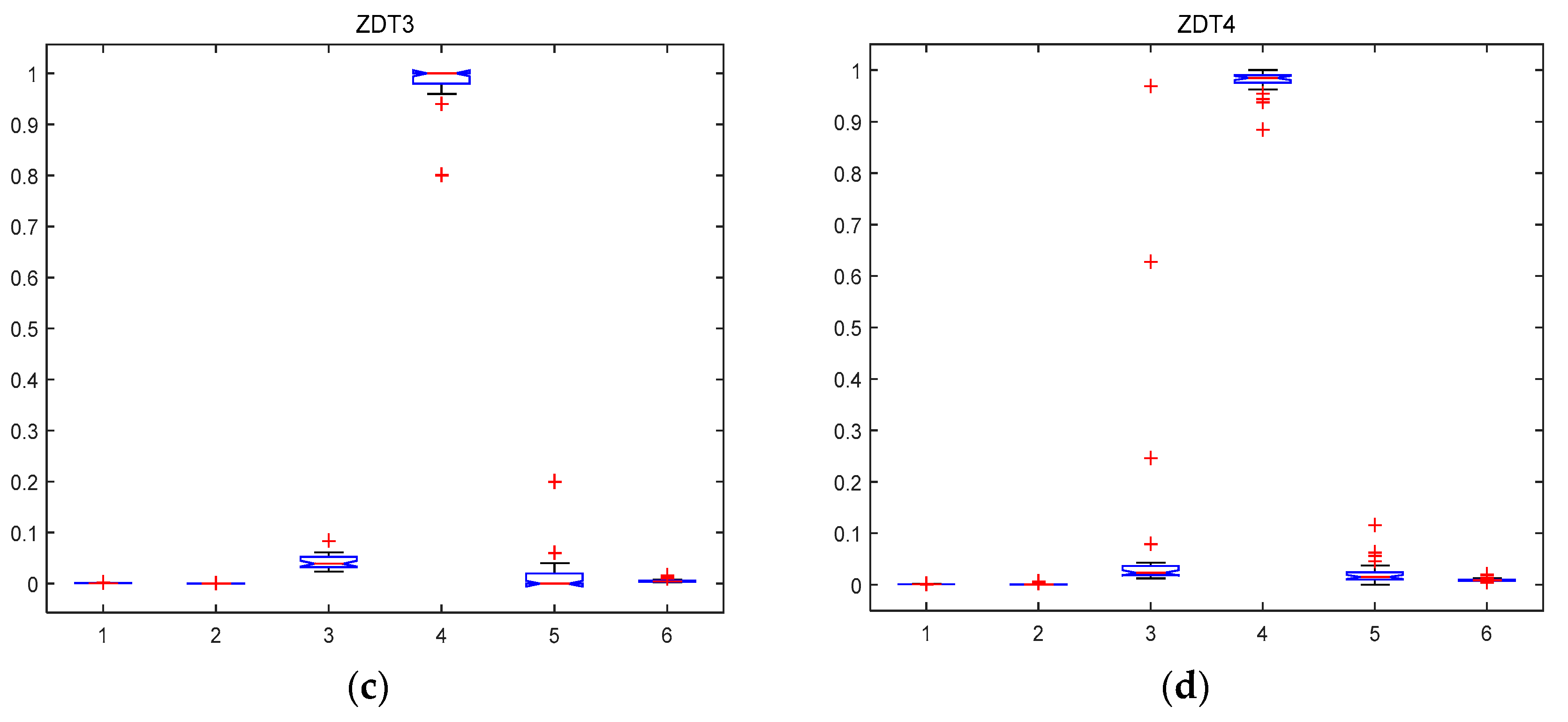
The performance of the MABBO for ZDTs in 30 independently runs by boxplot is shown in Figure 1. Boxplot displays box plots of multiple data samples. On each box, the central red line mark is the median, the edges of the box marked by blue line are the 25th and 75th percentiles, the whiskers extend to the most extreme data points the algorithm considers to be not outliers, and the outliers are plotted individually by red points. Figure 1 shows that the algorithm achieves great convergence, stable and well distributed solution sets in all the six metrics, and has a good performance for the ZDT1, ZDT2, ZDT3, and ZDT4 problems. As one can see, the medians of GD, GD standard deviation, SP, ER, and γ in each problem are very close to zero value, showing that the approximations obtained by MABBO are close to the Pareto-optimal fronts, and are well distributed. The CR metric on ZDT test problems also shows that all Pareto-optimal fronts were well covered. Also, the dispersion around the median in all cases is small, showing that the performance of MABBO was consistent with distributed points on the Pareto-optimal front for the ZDTs’ problems.
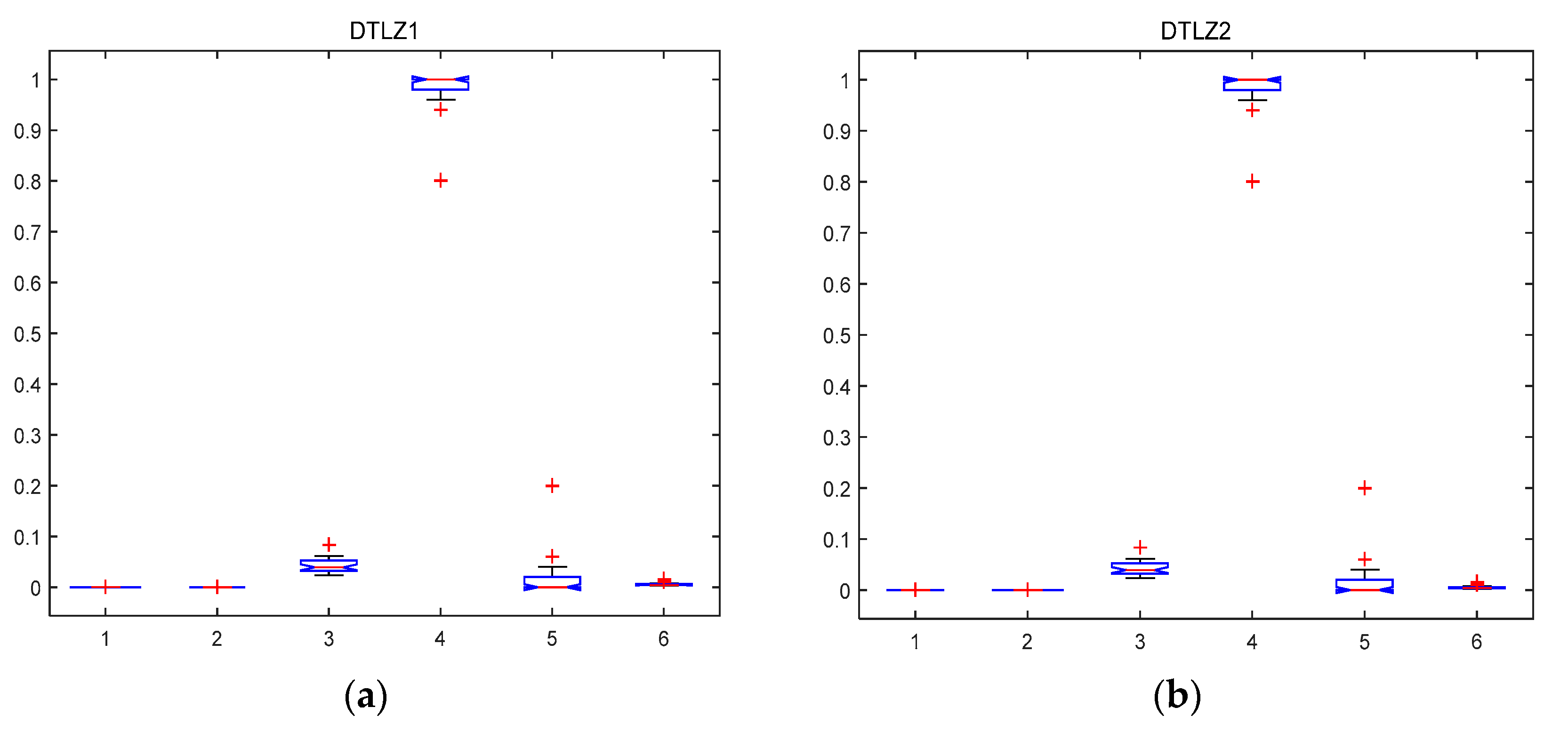
The performance of the MABBO was assessed with the following metrics: GD, GD standard deviation, SP, CR, ER, and γ. The performance of the MABBO on these metrics for DTLZs problems in 30 independently runs by boxplot is shown in Figure 2. the central red line mark on each box is the median, the edges of the box marked by blue line are the 25th and 75th percentiles, the whiskers extend to the most extreme data points the algorithm considers to be not outliers, and the outliers are plotted individually by red points. You can see that the median of the GD, GD standard deviation, SP and γ metrics are close to zero showing that the approximation to the Pareto-optimal front, and coverage rate of the solutions, is acceptable. Although the spacing metric may fluctuate a little at times on DTLZ4 test problem, γ metric still shows that solutions of Pareto-achieved front are pretty close to the Pareto-optimal front. Figure 2 shows good performance of the MABBO over six different metrics on four DTLZ test problems. The results show the distribution of the solutions, and the convergence to Pareto-optimal front. It indicates that our approach also performed well on 3-objective test problems.
5.2.2. The Comparison with other MOEAs
The experimental results of six algorithms on ZDT test problems are presented in Table 2. The rows of each algorithm give the mean value and standard deviation (shown in brackets) of each metric. As shown in Table 2, in terms of convergence, for ZDT1, ZDT3, and ZDT4, MABBO can get a smaller GD than the other five algorithms; for ZDT2, MABBO is better than the others, except for HMOEA and MOTLBO. Although HMOEA has a smaller GD value, the SP value of MABBO is less than HMOEA. The standard deviation of the GD value obtained by MABBO algorithm is the best of the six algorithms on ZDT test problems. It is shown that MABBO has better convergence performance compared with other algorithms. In terms of distribution uniformity, the SP value obtained by MABBO algorithm is better than HMOEA and BBMO. Although MOTLBO and NSGA-II have smaller SP, the GD value of these two algorithms is much larger than that of MABBO. The results show that these two algorithms have better distribution uniformity, but its convergence is not as good as MABBO. The distribution of the MABBO on the ZDT test problems can make the approximate Pareto optimal solution set and maintain the diversity of population better.
The experimental results of six algorithms on DTLZ test problems are presented in Table 3. Interms of convergence, for DTLZ 1, DTLZ 4 and DTLZ7 test problems, MABBO can get a smaller GD than the other five algorithms; for DTLZ2, MABBO is better than other algorithms except for HMOEA. It is shown that MABBO has better convergence performance compared with other algorithms. In terms of distribution uniformity, for DTLZ1, SP values obtained by MABBO algorithm are the smallest. For DTLZ2, DTLZ 4, and DTLZ7 test problems, the SP value obtained by MABBO algorithm is almost same as other algorithms. It can be seen from Table 3 that MABBO algorithm on the three objective test functions (DTLZ) obtains a smaller GD value and SP value than other algorithms. Compared with Table 2, MABBO algorithm used in DTLZ test problems has a better performance than in ZDT test problems. Therefore, the performance on the three objective functions is better than compared to two. The performance is not obviously decreased with the increased dimension of the problem.
We also find that to some extent, the more loops that are done, the better the GD result will be. If we remove D(i) from Equation (10), the spacing metric can improve a lot, but the GD result can also be worse. Computing the metrics with a large number of loops can improve the performance of MABBO algorithm. In brief, from Table 2 and Table 3, it can be seen that MABBO algorithm used in multi-objective benchmark functions has better performance than other algorithms.
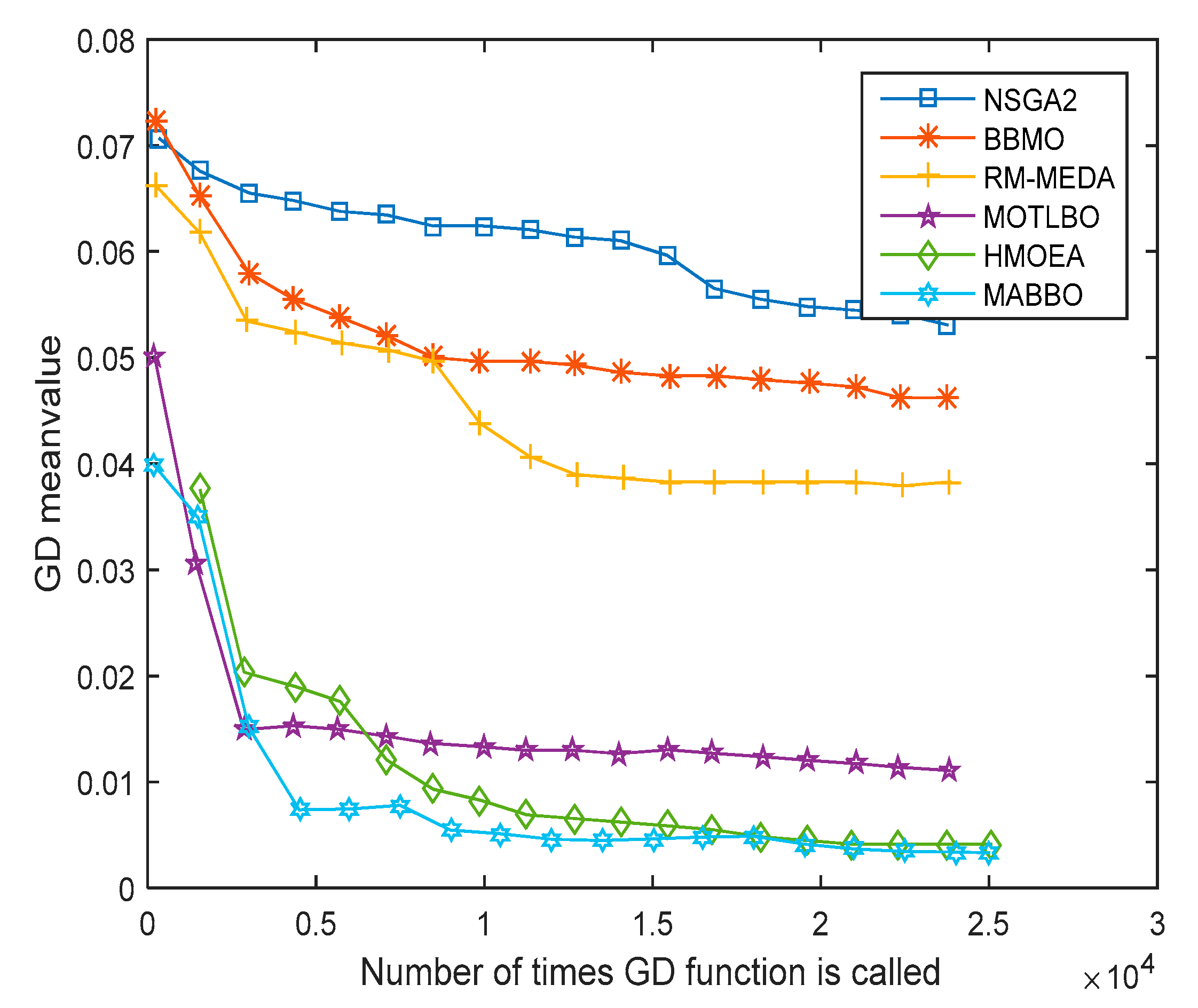
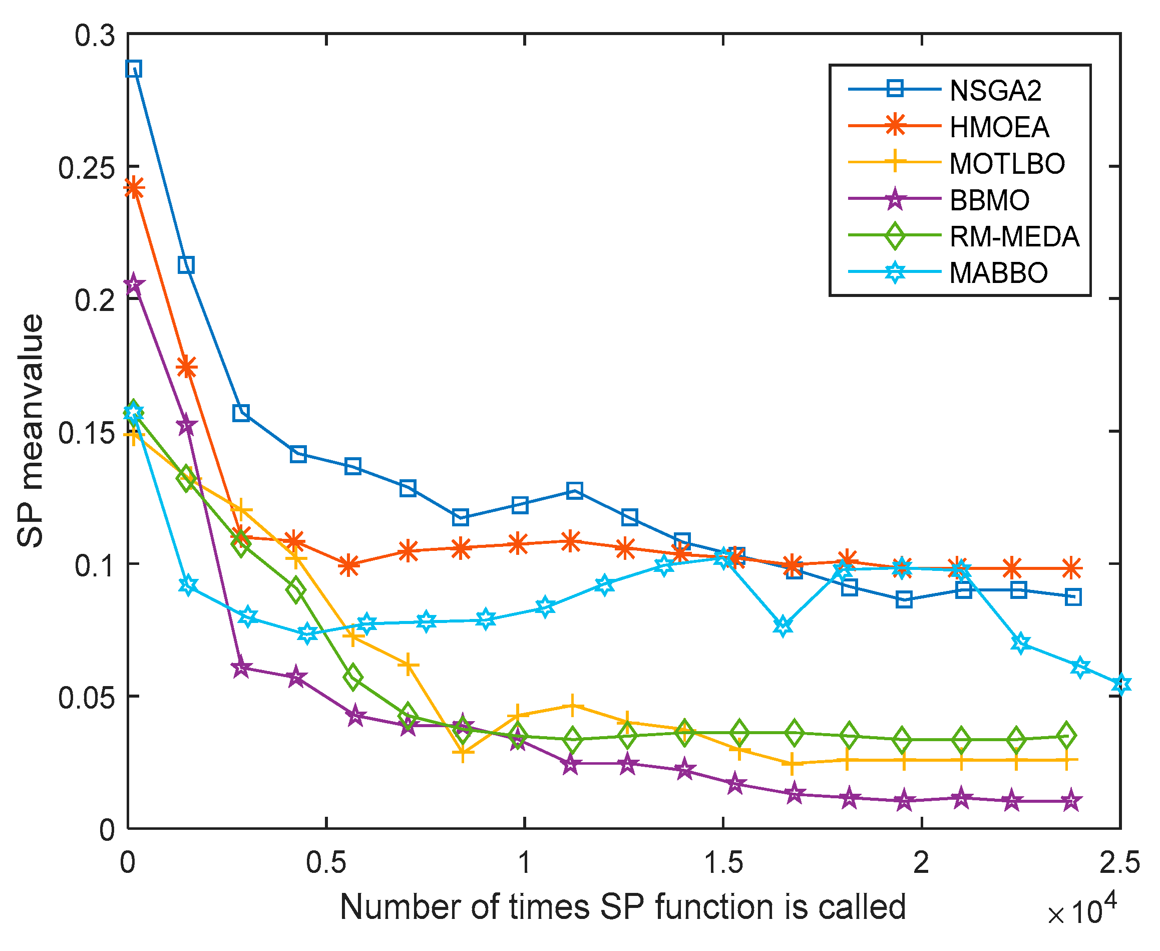
In order to measure further the efficiency of each algorithm, the GD and SP value obtained by the six algorithms on different test functions are compared. Due to the limitations of pages, the results obtained by the six different algorithms used to the test DTLZ2 problem are given in Figure 3 and Figure 4.
It can be seen from Figure 3, when the number of times of GD function called is 10,000, these three methods, that is MABBO, HMOEA and MOTLBO, can obtain a smaller GD value. It can be seen that the convergence speed of these three algorithms is significantly faster than the other three algorithms. When the number of times of GD function called reaches 5000, MABBO first obtains the smallest GD. After the number of times of GD function called reaches 14,000, the convergence of MOTLBO appears to be stagnant, and its GD value is worse than MABBO and HMOEA. It can be seen that MABBO and HMOEA have great advantages in convergence speed and convergence precision, than the other algorithms.
As can be seen from Figure 4, when the number of times of SP function called reaches 2000, MABBO first obtains the smallest SP value. Its SP value then always maintains a smaller value. It can be seen that MABBO is faster than the other five algorithms in optimizing the distribution of the solution set. The SP value of MABBO for DTLZ2 test problem fluctuates and rises in the middle of the evaluations, but dropped as expected in the end, and worked better than NSGA2 and HMOEA. In the future research work, the performance of the algorithm on the SP value will be further considered for improvement. Figure 3 and Figure 4 show that MABBO has higher efficiency. Based on the above analysis, for ZDT and DTLZ test problems, MABBO has obvious advantages compared with the other five algorithms for the convergence of the solution set, and it also has better performance on the uniformity of the distribution.
6. Conclusions
In view of the poor convergence solution set and distribution uniformity of existing multi-objective evolutionary algorithm in solving complex multi-objective optimization problems, a hybrid optimization algorithm, named MABBO, based on biogeography-based optimization, has been proposed. The new algorithm incorporates DE into the mutation procedure, moreover, a new migration operator based on number of iterations has been used to improve performance. Simultaneously, migration probability and mutation probability are adaptively changed according to the relation between the cost of fitness function of randomly selected habitats and average cost of fitness function of all habitats of last generation. Meanwhile, according to the evolutionary mechanism of BBO, the habitat suitability index, which combines with the Pareto dominance relation and density information between the habitat individuals, is redefined. Experiments are performed on ZDT and DTLZ, and benchmark functions are compared with the existing MOEAs; the results show that the obtained Pareto solution set can approximate to the Pareto optimal front, and has good diversity and uniform distribution. The results also demonstrate that the MABBO algorithm, which has been proposed to solve the multi-objective optimization problem, has better performance in convergence and distribution. In future research work, we will apply the MABBO algorithm to the motif discovery problem in biology, and verify the effectiveness of the algorithm in practical applications.
Acknowledgments
We gratefully acknowledge the support of the Joint Funds of the National Natural Science Foundation of China (No. 61462022, No.11561017), Major Science and Technology Project of Hainan Province (ZDKJ2016015), Natural Science Foundation of Hainan province of China (No. 20156226) and Hainan University scientific research foundation (No.kyqd1533) in carrying out this research.
Author Contributions
Siling Feng contributed the new processing method, conceived and designed the experiments; Siling Feng and Ziqiang Yang performed the experiments; Siling Feng and Ziqiang Yang analyzed the data; Mengxing Huang contributed analysis tools; and Siling Feng wrote the paper.
Conflicts of Interest
The authors declare no conflict of interest.
References
- Simon, D. Biogeography-based optimization. IEEE Trans. Evol. Comput. 2008, 12, 702–713. [Google Scholar] [CrossRef]
- Boussaïd, I.; Chatterjee, A.; Siarry, P.; Ahmed-Nacer, M. (BBO/DE) With Differential Evolution for Optimal Power Allocation in Wireless Sensor Networks. IEEE Trans. Veh. Technol. 2011, 60, 2347–2353. [Google Scholar] [CrossRef]
- Zubair, A.; Malhotra, D.; Muhuri, P.K.; Lohani, Q.D. Hybrid Biogeography-Based Optimization for solving Vendor Managed Inventory System. In Proceedings of the IEEE Congress on Evolutionary Computation 2017, San Sebastián, Spain, 5–8 June 2017; pp. 2598–2605. [Google Scholar]
- Zhang, M.; Zhang, B.; Zheng, Y. Bio-Inspired Meta-Heuristics for Emergency Transportation Problems. Algorithms 2014, 7, 15–31. [Google Scholar] [CrossRef]
- Khishe, M.; Mosavi, M.R.; Kaveh, M. Improved migration models of biogeography-based optimization for sonar dataset classification by using neural network. Appl. Acoust. 2017, 118, 15–29. [Google Scholar] [CrossRef]
- Wang, X.; Xu, Z.D. Multi-objective optimization algorithm based on biogeography with chaos. Int. J. Hybrid. Inf. Technol. 2014, 7, 225–234. [Google Scholar] [CrossRef]
- Bi, X.J.; Wang, J.; Li, B. Multi-objective optimization based on hybrid biogeography-based optimization. Syst. Eng. Electron. 2014, 36, 179–186. [Google Scholar]
- Vincenzi, L.; Savoia, M. Coupling response surface and differential evolution for parameter identification problems. Comput.-Aided Civ. Infrastruct. Eng. 2015, 30, 376–393. [Google Scholar] [CrossRef]
- Trivedi, A.; Srinivasan, D.; Biswas, S.; Reindl, T. Hybridizing genetic algorithm with differential evolution for solving the unit commitment scheduling problem. Swarm Evol. Comput. 2015, 23, 50–64. [Google Scholar] [CrossRef]
- Simon, D.; Mehmet, E.; Dawei, D.; Rick, R. Markov Models for Biogeography-Based Optimization. IEEE Trans. Syst., Man Cybern B Cybern. 2011, 41, 299–306. [Google Scholar] [CrossRef] [PubMed]
- Simon, D. A probabilistic analysis of a simplified biogeography-based optimization algorithm. Evol. Comput. 2011, 19, 167–188. [Google Scholar] [CrossRef] [PubMed]
- Ma, H.; Simon, D. Analysis of migration models of biogeography-based optimization using Markov theory. Eng. Appl. Artif. Intell. 2011, 24, 1052–1060. [Google Scholar] [CrossRef]
- Boussaïd, I.; Chatterjee, A.; Siarry, P.; Ahmed-Nacer, M. Two-stage update biogeography-based optimization using differential evolution algorithm (DBBO). Comput. Oper. Res. 2011, 38, 1188–1198. [Google Scholar] [CrossRef]
- Jiang, W.; Shi, Y.; Zhao, W.; Wang, X. Parameters Identification of Fluxgate Magnetic Core Adopting the Biogeography-Based Optimization Algorithm. Sensors 2016, 16, 979. [Google Scholar] [CrossRef] [PubMed]
- Gong, W.; Cai, Z.; Ling, C.X. DE/BBO: A hybrid differential evolution with biogeography-based optimization for global numerical optimization. Soft Comput. 2010, 15, 645–665. [Google Scholar] [CrossRef]
- Ma, H.; Simon, D. Blended biogeography-based optimization for constrained optimization. Eng. Appl. Artif. Intell. 2011, 24, 517–525. [Google Scholar] [CrossRef]
- Li, X.; Wang, J.; Zhou, J.; Yin, M. A perturb biogeography based optimization with mutation for global numerical optimization. Appl. Math. Comput. 2011, 218, 598–609. [Google Scholar] [CrossRef]
- Ergezer, M.; Simon, D.; Du, D. Oppositional biogeography-based optimization. In Proceedings of the 2009 IEEE International Conference on Systems, Man and Cybernetics, San Antonio, TX, USA, 11–14 October 2009; pp. 1009–1014. [Google Scholar] [CrossRef]
- Tan, L.; Guo, L. Quantum and biogeography based optimization for a class of combinatorial optimization. In Proceedings of the first ACM/SIGEVO Summit on Genetic and Evolutionary Computation—GEC2009, Shanghai, China, 12–14 June 2009; ACM: New York, NY, USA, 2009; Volume 2, p. 969. [Google Scholar] [CrossRef]
- Gong, W.; Cai, Z.; Ling, C.X.; Li, H. A real-coded biogeography-based optimization with mutation. Appl. Math. Comput. 2010, 216, 2749–2758. [Google Scholar] [CrossRef]
- Bhattacharya, A.; Chattopadhyay, P.K. Hybrid Differential Evolution with Biogeography-Based Optimization for Solution of Economic Load Dispatch. IEEE Trans. Power Syst. 2010, 2, 1955–1964. [Google Scholar] [CrossRef]
- Majumdar, K.; Das, P.; Roy, P.K.; Banerjee, S. Solving OPF Problems using Biogeography Based and Grey Wolf Optimization Techniques. Int. J. Energy Optim. Eng. 2017, 6, 55–77. [Google Scholar] [CrossRef]
- Sun, G.; Liu, Y.; Liang, S.; Wang, A.; Zhang, Y. Beam pattern design of circular antenna array via efficient biogeography-based optimization. AEU-Int. J. Electron. Commun. 2017, 79, 275–285. [Google Scholar] [CrossRef]
- Liu, F.; Nakamura, K.; Payne, R. Abnormal Breast Detection via Combination of Particle Swarm Optimization and Biogeography-Based Optimization. In Proceedings of the 2nd International Conference on Mechatronics Engineering and Information Technology, ICMEIT 2017, Dalian, China, 13–14 May 2017. [Google Scholar]
- Johal, N.K.; Singh, S.; Kundra, H. A hybrid FPAB/BBO Algorithm for Satellite Image Classification. Int. J. Comput. Appl. 2010, 6, 31–36. [Google Scholar] [CrossRef]
- Song, Y.; Liu, M.; Wang, Z. Biogeography-Based Optimization for the Traveling Salesman Problems. In Proceedings of the 2010 Third International Joint Conference on Computational Science and Optimization, Huangshan, China, 28–31 May 2010; pp. 295–299. [Google Scholar] [CrossRef]
- Mo, H.; Xu, L. Biogeography Migration Algorithm for Traveling Salesman Problems; Springer: Berlin/Heidelberg, Germany, 2010; pp. 405–414. [Google Scholar]
- Silva, M.A.C.; Coelho, L.S.; Freire, R.Z. Biogeography-based Optimization approach based on Predator-Prey concepts applied to path planning of 3-DOF robot manipulator. In Proceedings of the 2010 IEEE 15th Conference on Emerging Technologies & Factory Automation (ETFA 2010), Bilbao, Spain, 13–16 September 2010; pp. 1–8. [Google Scholar]
- Lohokare, M.R.; Pattnaik, S.S.; Devi, S.; Panigrahi, B.K.; Das, S.; Jadhav, D.G. Discrete Variables Function Optimization Using Accelerated Biogeography-Based Optimization; Springer: Berlin/Heidelberg, Germany, 2010; pp. 322–329. [Google Scholar]
- Boussaid, I.; Chatterjee, A.; Siarry, P.; Ahmed-Nacer, M. Hybridizing biogeography-based optimization with differential evolution for optimal power allocation in wireless sensor networks. IEEE Trans. Veh. Technol. 2011, 60, 2347–2353. [Google Scholar] [CrossRef]
- Wang, L.; Xu, Y. An effective hybrid biogeography-based optimization algorithm for parameter estimation of chaotic systems. Expert. Syst. Appl. 2011, 38, 15103–15109. [Google Scholar] [CrossRef]
- Ovreiu, M.; Simon, D. Biogeography-based optimization of neuro-fuzzy system parameters for diagnosis of cardiac disease. In Proceedings of the 12th annual conference on Genetic and evolutionary computation—GECCO2010, Portland, OR, USA, 7–11 July 2010; ACM: New York, NY, USA; p. 1235. [Google Scholar] [CrossRef]
- Yin, M.; Li, X. Full Length Research Paper A hybrid bio-geography based optimization for permutation flow shop scheduling. Sci. Res. Essays 2011, 6, 2078–2100. [Google Scholar]
- Reddy, S.S.; Kumari, M.S.; Sydulu, M. Congestion management in deregulated power system by optimal choice and allocation of FACTS controllers using multi-objective genetic algorithm. In Proceedings of the 2010 IEEE PES T&D, New Orleans, LA, USA, 19–22 April 2010; pp. 1–7. [Google Scholar] [CrossRef]
- Reddy, S.S.; Abhyankar, A.R.; Bijwe, P.R. Reactive power price clearing using multi-objective optimization. Energy 2011, 36, 3579–3589. [Google Scholar] [CrossRef]
- Reddy, S.S. Multi-objective based congestion management using generation rescheduling and load shedding. IEEE Trans. Power Syst. 2017, 32, 852–863. [Google Scholar] [CrossRef]
- Reddy, S.S.; Bijwe, P.R. Multi-Objective Optimal Power Flow Using Efficient Evolutionary Algorithm. Int. J. Emerg. Electr. Power Syst. 2017, 18. [Google Scholar] [CrossRef]
- Silva, M.A.C.; Coelho, L.S.; Lebensztajn, L. Multi objective biogeography-based optimization based on predator-prey approach. IEEE Trans. Magn. 2012, 48, 951–954. [Google Scholar] [CrossRef]
- Goudos, S.K.; Plets, D.; Liu, N.; Martens, L.; Joseph, W. A multi-objective approach to indoor wireless heterogeneous networks planning based on biogeography-based optimization. Comput. Netw. 2015, 91, 564–576. [Google Scholar] [CrossRef]
- Ma, H.P.; Su, S.F.; Simon, D.; Fei, M.R. Ensemble multi-objective biogeography-based optimization withapplication to automated warehouse scheduling. Eng. Appl. Artif. Intell. 2015, 44, 79–90. [Google Scholar] [CrossRef]
- Reihanian, A.; Feizi-Derakhshi, M.-R.; Aghdasi, H.S. Community detection in social networks with node attributes based on multi-objective biogeography based optimization. Eng. Appl. Artif. Intell. 2017, 62, 51–67. [Google Scholar] [CrossRef]
- Guo, W.A.; Wang, L.; Wu, Q.D. Numerical comparisons of migration models for Multi-objective Biogeography-Based Optimization. Inf. Sci. 2016, 328, 302–320. [Google Scholar] [CrossRef]
- Ma, H.; Yang, Z.; You, P.; Fei, M. Multi-objective biogeography-based optimization for dynamic economic emission load dispatch considering plug-in electric vehicles charging. Energy 2017, 135, 101–111. [Google Scholar] [CrossRef]
- Gachhayat, S.K.; Dash, S.K. Non-Convex Multi Objective Economic Dispatch Using Ramp Rate Biogeography Based Optimization. Int. J. Electr. Comput. Energetic Electron. Commun. Eng. 2017, 11, 545–549. [Google Scholar]
- Zheng, Y.-J.; Wang, Y.; Ling, H.-F.; Xue, Y.; Chen, S.-Y. Integrated civilian–military pre-positioning of emergency supplies: A multi-objective optimization approach. Appl. Soft Comput. 2017, 58, 732–741. [Google Scholar] [CrossRef]
- Veldhuizen, D.A.V.; Lamont, G.B. Evolutionary computation and convergence to a pareto front. In Late Breaking Papers at the Genetic Programming; Koza, J.R., Ed.; Stanford Bookstore: Stanford, CA, USA, 1998; pp. 221–228. [Google Scholar]
- Schott, J.R. Fault tolerant design using single and multi-criteria genetic algorithm optimization. Master’s Thesis, Massachusetts Institute of Technology, Cambridge, MA, USA, 1995. [Google Scholar]
- Zitzler, E.; Thiele, L. Multiobjective evolutionary algorithms: A comparative case study and the strength pareto approach. IEEE Trans. Evol. Comput. 1999, 3, 257–271. [Google Scholar] [CrossRef]
- Deb, K.; Pratap, A.; Agarwal, S. A fast and elitist multi-objective genetic algorithm: NSGA-II. IEEE Trans. Evol. Comput. 2002, 6, 182–197. [Google Scholar] [CrossRef]
- Zhang, Q.F.; Zhou, A.M.; Jin, Y.C. RM-MEDA: A regularity model-based multi-objective estimation of distribution algorithm. IEEE Trans. Evol. Comput. 2008, 12, 41–63. [Google Scholar] [CrossRef]
- Zou, F.; Wang, L.; Hei, X. Multi-objective optimization using teaching-learning-based optimization algorithm. Eng. Appl. Artif. Intel. 2013, 26, 1291–1300. [Google Scholar] [CrossRef]
- Tang, L.X.; Wang, X.P. A hybrid multi-objective evolutionary algorithm for multiobjective optimization problems. IEEE Trans. Evol. Comput. 2013, 17, 20–45. [Google Scholar] [CrossRef]
- Ma, H.; Ruan, X.; Pan, Z. Handling multiple objectives with biogeography-based optimization. Int. J. Autom. Comput. 2012, 9, 30–36. [Google Scholar] [CrossRef]
- Deb, K.; Thiele, L.; Laumanns, M.; Zitzler, E. Scalable Multi-Objective Optimization Test Problems. In Proceedings of the CEC 2002, Honolulu, HI, USA, 12–17 May 2002; pp. 825–830. [Google Scholar]
Figure 1.
Box plot representing the distribution of the metrics on ZDT test problems (GD = 1, standard deviation of GD = 2, SP = 3, CR = 4, ER = 5 and γ = 6). (a) the metrics on ZDT1 problem; (b) the metrics on ZDT2 problem; (c) the metrics on ZDT3 problem; (d) the metrics on ZDT4 problem.
Figure 1.
Box plot representing the distribution of the metrics on ZDT test problems (GD = 1, standard deviation of GD = 2, SP = 3, CR = 4, ER = 5 and γ = 6). (a) the metrics on ZDT1 problem; (b) the metrics on ZDT2 problem; (c) the metrics on ZDT3 problem; (d) the metrics on ZDT4 problem.
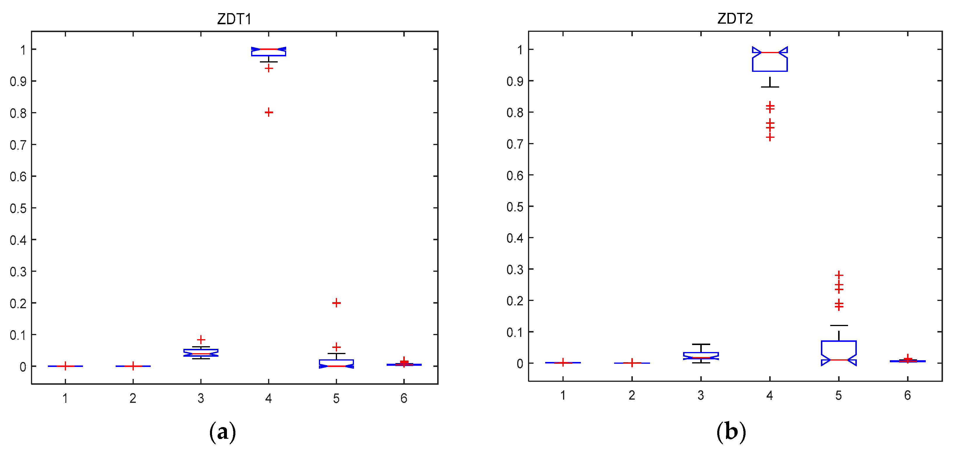

Figure 2.
Boxplot representing the distribution of the metrics on DTLZ test problems (GD = 1, standard deviation of GD = 2, SP = 3, CR = 4, ER = 5 and γ = 6). (a) the metrics on DTLZ1 problem; (b) the metrics on DTLZ2 problem; (c) the metrics on DTLZ4 problem; (d) the metrics on DTLZ7 problem.
Figure 2.
Boxplot representing the distribution of the metrics on DTLZ test problems (GD = 1, standard deviation of GD = 2, SP = 3, CR = 4, ER = 5 and γ = 6). (a) the metrics on DTLZ1 problem; (b) the metrics on DTLZ2 problem; (c) the metrics on DTLZ4 problem; (d) the metrics on DTLZ7 problem.

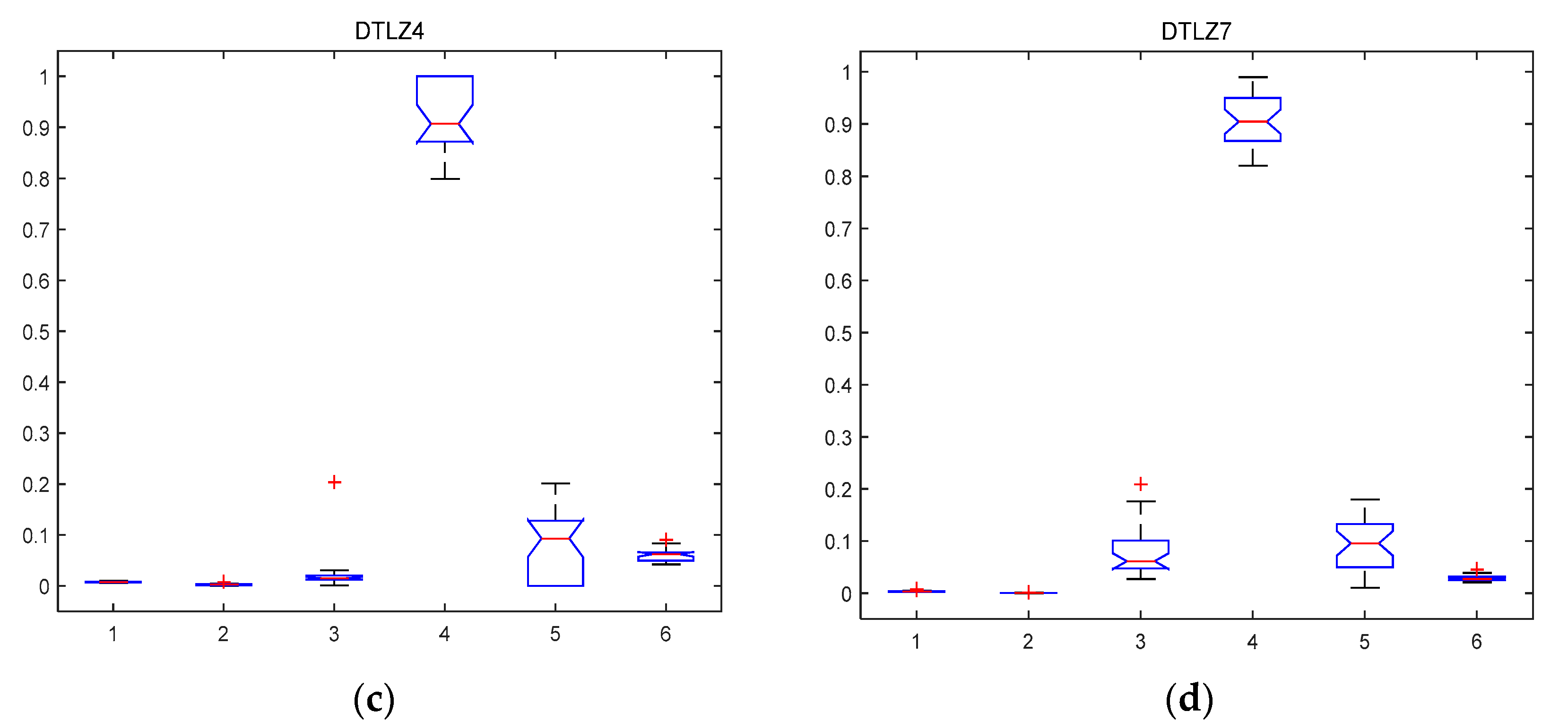
Figure 3.
The GD index of six algorithms on DTLZ2 test problem.

Figure 4.
The SP index of six algorithms on DTLZ2 test problem.


Table 1.
Parameters used by test problems.
| Function | ZDT1 | ZDT2 | ZDT3 | ZDT4 | DTLZ1 | DTLZ2 | DTLZ4 | DTLZ7 |
|---|---|---|---|---|---|---|---|---|
| Popsize | 100 | 100 | 100 | 100 | 100 | 100 | 100 | 100 |
| NumVar | 30 | 30 | 10 | 10 | 10 | 10 | 10 | 22 |
| Pmodify | 0.75 | 0.75 | 0.75 | 0.75 | 0.75 | 0.75 | 0.75 | 0.75 |
| Pmutation | 0.05 | 0.005 | 0.005 | 0.005 | 0.2 | 0.005 | 0.005 | 0.05 |
| Elitismkeep | 15 | 15 | 15 | 15 | 10 | 15 | 10 | 10 |
| k1 | 0.4 | 0.4 | 0.4 | 0.4 | 0.4 | 0.4 | 0.4 | 0.4 |
| k2 | 0.95 | 0.95 | 0.95 | 0.95 | 0.95 | 0.95 | 0.95 | 0.95 |
| k3 | 0.1 | 0.1 | 0.1 | 0.1 | 0.1 | 0.1 | 0.1 | 0.1 |
| k4 | 0.25 | 0.25 | 0.25 | 0.25 | 0.25 | 0.25 | 0.25 | 0.25 |
| Generation | 100 | 100 | 100 | 100 | 100 | 100 | 100 | 100 |
| PerLoop | 100 | 100 | 100 | 100 | 10 | 10 | 10 | 10 |
Table 2.
Comparison on 2-objective test problems (ZDTs).
| Algorithm | ZDT1 | ZDT2 | ZDT3 | ZDT4 | ||||
|---|---|---|---|---|---|---|---|---|
| GD | SP | GD | SP | GD | SP | GD | SP | |
| MABBO | 8.44 × 10⁻⁴ | 2.33 × 10⁻² | 1.28 × 10⁻³ | 4.37 × 10⁻² | 7.22 × 10⁻⁴ | 4.29 × 10⁻² | 9.64 × 10⁻⁴ | 8.47 × 10⁻² |
| (2.91 × 10⁻⁵) | (1.56 × 10⁻²) | (4.18 × 10⁻⁵) | (7.43 × 10⁻²) | (2.49 × 10⁻⁵) | (1.34 × 10⁻²) | (5.55 × 10⁻⁴) | (2.03 × 10⁻¹) | |
| NSGA-II | 2.93 × 10⁻³ | 7.79 × 10⁻³ | 1.85 × 10⁻³ | 7.41 × 10⁻³ | 1.78 × 10⁻³ | 8.42 × 100 | 6.34 × 10⁻³ | 9.73 × 10⁻³ |
| (4.74 × 10⁻⁴) | (7.40 × 10⁻³) | (2.99 × 10⁻³) | (6.57 × 10⁻³) | (4.75 × 10⁻³) | (1.75 × 10⁻³) | (3.96 × 10⁻³) | (5.32 × 10⁻³) | |
| BBMO | 2.53 × 10⁻² | 2.74 × 10⁻² | 3.26 × 10⁻² | 7.88 × 10⁻¹ | 7.23 × 10⁻² | 4.93 × 10⁻³ | 3.33 × 10⁻² | 4.16 × 10⁻² |
| (2.98 × 10⁻³) | (5.53 × 10⁻³) | (2.72 × 10⁻²) | (3.83 × 10⁻¹) | (1.41 × 10⁻²) | (1.65 × 10⁻³) | (6.51 × 10⁻³) | (1.31 × 10⁻²) | |
| RM-MEDA | 2.87 × 10⁻³ | 1.10 × 10⁻² | 4.76 × 10⁻³ | 3.88 × 10⁻³ | 2.17 × 10⁻³ | 1.19 × 10⁻² | 1.54 × 10⁻³ | 7.25 × 10⁻³ |
| (8.47 × 10⁻³) | (1.18 × 10⁻³) | (1.58 × 10⁻³) | (1.56 × 10⁻³) | (9.01 × 10⁻³) | (2.80 × 10⁻³) | (1.69 × 10⁻³) | (1.86 × 10⁻³) | |
| MOTLBO | 1.59 × 10⁻³ | 4.01 × 10⁻³ | 9.34 × 10⁻⁴ | 7.38 × 10⁻³ | 2.04 × 10⁻³ | 3.37 × 10⁻³ | 1.42 × 10⁻³ | 2.49 × 10⁻³ |
| (3.27 × 10⁻³) | (3.68 × 10⁻³) | (1.06 × 10⁻³) | (6.96 × 10⁻³) | (8.47 × 10⁻⁴) | (3.08 × 10⁻³) | (2.49 × 10⁻³) | (2.74 × 10⁻⁴) | |
| HMOEA | 3.74 × 10⁻⁴ | 5.75 × 10⁻¹ | 3.06 × 10⁻⁴ | 7.23 × 10⁻¹ | 6.75 × 10⁻⁴ | 3.53 × 10⁻¹ | 1.14 × 10⁻³ | 3.91 × 10⁻¹ |
| (8.24 × 10⁻⁴) | (2.50 × 10⁻²) | (2.52 × 10⁻⁴) | (7.54 × 10⁻²) | (3.84 × 10⁻⁴) | (6.45 × 10⁻³) | (8.23 × 10⁻⁴) | (9.23 × 10⁻²) | |
Table 3.
Comparison on 3-objective test problems (DTLZs).
| Algorithm | DTLZ1 | DTLZ2 | DTLZ4 | DTLZ7 | ||||
|---|---|---|---|---|---|---|---|---|
| GD | SP | GD | SP | GD | SP | GD | SP | |
| MABBO | 5.84 × 10⁻³ | 2.96 × 10⁻² | 4.41 × 10⁻³ | 6.13 × 10⁻² | 7.57 × 10⁻³ | 2.81 × 10⁻² | 3.41 × 10⁻³ | 7.96 × 10⁻² |
| (1.09 × 10⁻⁴) | (9.33 × 10⁻³) | (1.22 × 10⁻⁴) | (2.21 × 10⁻²) | (2.69 × 10⁻³) | (4.80 × 10⁻²) | (3.99 × 10⁻⁴) | (4.74 × 10⁻²) | |
| NSGA-2 | 6.74 × 10⁻² | 3.68 × 10⁻¹ | 5.31 × 10⁻² | 8.51 × 10⁻² | 5.44 × 10⁻² | 2.09 × 10⁻² | 7.15 × 10⁻² | 6.63 × 10⁻² |
| (2.25 × 10⁻¹) | (1.66E × 100 | (1.72 × 10⁻³) | (5.76 × 10⁻²) | (6.09 × 10⁻²) | (5.14 × 10⁻²) | (3.43 × 10⁻²) | (2.19 × 10⁻²) | |
| BBMO | 6.34 × 10⁻² | 3.85 × 10⁻¹ | 4.81 × 10⁻² | 1.12 × 10⁻² | 2.45 × 10⁻¹ | 1.75 × 10⁻¹ | 1.42 × 10⁻¹ | 2.22 × 10⁻¹ |
| (1.17 × 10⁻¹) | (2.28 × 10⁻¹) | (5.22 × 10⁻²) | (3.95 × 10⁻²) | (3.75 × 10⁻²) | (2.75 × 10⁻²) | (2.75 × 10⁻²) | (1.07 × 10⁻¹) | |
| RM-MEDA | 3.76 × 10⁻² | 7.65 × 10⁻² | 3.54 × 10⁻² | 3.98 × 10⁻² | 7.73 × 10⁻² | 9.13 × 10⁻² | 1.18 × 10⁻² | 2.75 × 10⁻² |
| (9.45 × 10⁻²) | (4.53 × 10⁻¹) | (9.20 × 10⁻²) | (5.92 × 10⁻²) | (5.76 × 10⁻²) | (2.53 × 10⁻²) | (4.28 × 10⁻²) | (1.95 × 10⁻²) | |
| MOTLBO | 7.83 × 10⁻² | 8.34 × 10⁻² | 1.06 × 10⁻² | 2.46 × 10⁻² | 3.74 × 10⁻² | 3.30 × 10⁻² | 2.21 × 10⁻² | 3.34 × 10⁻² |
| (5.97 × 10⁻¹) | (8.13 × 10⁻²) | (4.92 × 10⁻³) | (3.66 × 10⁻³) | (4.99 × 10⁻²) | (3.06 × 10⁻²) | (5.54 × 10⁻³) | (7.92 × 10⁻²) | |
| HMOEA | 3.37 × 10⁻² | 3.04 × 10⁻¹ | 2.41 × 10⁻³ | 1.23 × 10⁻¹ | 2.23 × 10⁻² | 1.23 × 10⁻¹ | 4.84 × 10⁻³ | 5.38 × 10⁻¹ |
| (7.15 × 10⁻²) | (2.13 × 10⁻¹) | (6.78 × 10⁻³) | (2.86 × 10⁻²) | (1.78 × 10⁻²) | (3.38 × 10⁻²) | (9.02 × 10⁻³) | (5.44 × 10⁻²) | |
© 2017 by the authors. Licensee MDPI, Basel, Switzerland. This article is an open access article distributed under the terms and conditions of the Creative Commons Attribution (CC BY) license (http://creativecommons.org/licenses/by/4.0/).
Share and Cite
MDPI and ACS Style
Feng, S.; Yang, Z.; Huang, M. Hybridizing Adaptive Biogeography-Based Optimization with Differential Evolution for Multi-Objective Optimization Problems. Information 2017, 8, 83. https://doi.org/10.3390/info8030083
AMA Style
Feng S, Yang Z, Huang M. Hybridizing Adaptive Biogeography-Based Optimization with Differential Evolution for Multi-Objective Optimization Problems. Information. 2017; 8(3):83. https://doi.org/10.3390/info8030083
Chicago/Turabian StyleFeng, Siling, Ziqiang Yang, and Mengxing Huang. 2017. "Hybridizing Adaptive Biogeography-Based Optimization with Differential Evolution for Multi-Objective Optimization Problems" Information 8, no. 3: 83. https://doi.org/10.3390/info8030083
Note that from the first issue of 2016, this journal uses article numbers instead of page numbers. See further details here.