
Understanding the Impact of Human Mobility Patterns on Taxi Drivers’ Profitability Using Clustering Techniques: A Case Study in Wuhan, China

1
Intelligent Transportation Systems Research Center, Wuhan University of Technology, Wuhan 430063, China
2
Engineering Research Center of Transportation Safety, Ministry of Education, Wuhan 430063, China
3
National Engineering Research Center for Water Transportation Safety, Heping Road, Wuchang District, Wuhan 430063, Hubei, China
*
Author to whom correspondence should be addressed.
Information 2017, 8(2), 67; https://doi.org/10.3390/info8020067
Submission received: 17 April 2017
/
Revised: 15 June 2017
/
Accepted: 15 June 2017
/
Published: 19 June 2017
Abstract
:Taxi trajectories reflect human mobility over the urban roads’ network. Although taxi drivers cruise the same city streets, there is an observed variation in their daily profit. To reveal the reasons behind this issue, this study introduces a novel approach for investigating and understanding the impact of human mobility patterns (taxi drivers’ behavior) on daily drivers’ profit. Firstly, a K-means clustering method is adopted to group taxi drivers into three profitability groups according to their driving duration, driving distance and income. Secondly, the cruising trips and stopping spots for each profitability group are extracted. Thirdly, a comparison among the profitability groups in terms of spatial and temporal patterns on cruising trips and stopping spots is carried out. The comparison applied various methods including the mash map matching method and DBSCAN clustering method. Finally, an overall analysis of the results is discussed in detail. The results show that there is a significant relationship between human mobility patterns and taxi drivers’ profitability. High profitability drivers based on their experience earn more compared to other driver groups, as they know which places are more active to cruise and to stop and at what times. This study provides suggestions and insights for taxi companies and taxi drivers in order to increase their daily income and to enhance the efficiency of the taxi industry.
1. Introduction
Taxis play a significant role in the travels of residents, tourists and other road users in the urban transportation system. A significant number of people are traveling by taxis in their daily movements around the world. According to a report issued in 2013 [1], taxi passengers’ traffic in 2012 recorded 387 million passengers; the daily passenger travel mileage increased by 2.4%. In addition, taxi idle rate decreased, and the empty-loading ratio was 29.6%. These numbers imply the yearly increment of occupancy frequency of taxi service in Wuhan City.
Although taxi drivers cruise the same streets, there is an observed variation in their incomes. The main reason behind this is taxi drivers freely plan and select their own routes once they drop off passengers and look for new passengers [2].
Previously, many surveys were conducted to understand taxi drivers’ mobility patterns and resulted in that there is a strong variation in taxis’ drivers’ incomes according to drivers’ skills and other factors. A survey [3] found that a skilled driver can earn 63% more than an average driver and more than twice that of a poorly-skilled driver. A questionnaire-based study [4] reported that there is a relationship between income and three factors, including length of time driving, weather (winter) and fuel prices.
As survey-based results of taxi related studies may be insufficient and could be biased, an alternative method is adopted by taking advantage of the taxi GPS technique, which is available in modern GPS-based dispatch systems. Human mobility patterns (also known as driver behavior patterns) of taxi drivers can be detected by investigating their spatial and temporal distribution and patterns using daily trajectory data. Many research works and studies have been conducted to investigate taxi drivers’ mobility patterns. Liu et al. [5] proposed a method for the analysis of taxi drivers’ operation behavior in a real urban environment. In their method, they studied large-scale cabdrivers’ behavior in urban areas with 3000 taxis in a metropolitan area. In addition, they provide an effective method for studying cabdrivers’ operation patterns.
The paper [6] presents a study to reveal the impact of social propagation for better prediction of cab drivers’ future behaviors. The study investigates the correlation between drivers’ skills and their mutual interactions in the latent vehicle-to-vehicle network. Wenxin Yang et al. [7] proposed a route recommendation algorithm based on a temporal probability grid network to increase the profit for taxi drivers. The proposed algorithm applied a map-reduce method to assist in reducing the taxi cruising distances. Powell et al. [8] measured the profitability of each area in terms of fare gains of all occupied taxi trips originating from that area, the number of trips and the cost from the current location to that area, exploiting the knowledge of passenger’s mobility patterns and taxi drivers’ pick-up/drop-off behaviors inferred from taxi GPS traces.
A visualization framework is developed to analyze and visualize a large amount of spatial-temporal and multi-dimensional trajectory data and to determine some key parameters that influence drivers according to their income [9]. Bing Zhu and Xin Xu [10] studied urban traffic patterns based on the taxi trajectories, especially the principal Origin-Destination traffic flow (OD flow) extraction. The paper focused on the picking-up and dropping-off events, and the issue is solved by a spatiotemporal density-based clustering method. The OD flow analysis is formulated as a 4D node clustering problem, and the relative distance function between two OD flows is defined, including a clustering preference factor, which is adjustable according to the observation scale favored. The authors in [11,12] provide methods to visualize and analyze the spatiotemporal driving patterns of the GPS taxi driver in order to present the significant social and economic impacts of human mobility on the urban areas.
Many previous studies considered GPS data clustering methods to provide recommendations to taxi drivers. Kumar et al. adopted a clustering method for grouping the origin-destination pairs of the taxi passengers in order to investigate city mobility patterns, urban hot-spots and road network usage of the crowd movement. A clustering sampling scheme (named cluVAT clustering sampling scheme visual assessment of cluster tendency) is used to obtain coarse clusters that represent crowd movement and reduce the data points that are not captured by the coarse clusters [13]. Chen et al. [14,15] proposed a two-phase approach for two-directional night bus route planning. In the first phase was a method for clustering “hot” areas with dense passenger pick-ups/drop-offs, and then, the large hot areas were split into smaller clusters and candidate bus stops represented by these clusters. In the second phase, bus stops and bus route graphs were chosen by a proposed method using the bus route origin, destination, candidate bus stops and bus operation time constraints. Shen et al. present an analysis and visualization method based on a city’s short-dated taxi GPS traces in order to provide recommendations for assisting cruising taxi drivers to find passengers using optimal routes. Recommended routes are obtained by adopting two steps: an improved DBSCAN clustering method and trajectories clustering. The hot spots for loading and unloading passenger(s) are extracted using an improved DBSCAN algorithm after data preprocessing, including cleaning and filtering. Then, the start-end point-based similar trajectory method is adopted to identify coarse-level trajectory clusters and then obtaining the recommended routes [16]. Chang et al. proposed an approach for recommending pick-up locations for taxi drivers. The approach extracted the demand requests according to the time, location and weather context and then clustered these requests into hotspots by the K-means, agglomerative hierarchical clustering and DBSCAN methods. Finally, the top-ranked places are recommended to taxi drivers according to a ranking method [17]. The authors in [18] used the trajectory data of taxis’ GPS to obtain a large volume of trips of anonymous customers in order to identify the patterns of intra-urban human mobility. The result of their study indicates that the geographical heterogeneity and distance decay effect improvement have an influence on human mobility patterns. Liu et al. [19] utilized a huge amount of taxi GPS data to investigate the relationship between traffic patterns and urban land uses. The temporal variations of pick-ups and drop-offs and their association with different land use features have been explored. Tang et al. [20] introduced an approach for analyzing travel demand distributions and searching behavior using taxi GPS data. The DBSCAN clustering method is adopted to cluster pick-up and drop-off locations. Travel distance, time and average speed are utilized to explore human mobility by extracting taxi trips from GPS trace data.
Previous studies have not comprehensively investigated the significant correlation between drivers’ behaviors and drivers’ profit. If we can reveal the correlation between the spatial and temporal pattern of taxi drivers and their profit, we may provide insights and suggestions for the taxi industry and taxi drivers in order to increase their overall income, and then, we may provide suggestions and insights for taxi companies and taxi drivers in order to increase their daily income and to enhance the efficiency of the taxi industry.
There is a need to present a novel approach to investigate and analyze the spatial and temporal patterns of taxi drivers especially when a taxi becomes empty. In this case, a taxi driver can freely select and cruise routes according to driving skills and experience, which may influence occupancy, oil consumption and daily income.
The main contribution of this study is presenting a novel approach for investigating and understanding the impact of human mobility patterns (taxi drivers’ behavior) on drivers’ profitability. Firstly, the K-means clustering method, for grouping taxi drivers into three groups according to three profitability features, is introduced. Secondly, cruising trips and stopping spots are extracted for each profitability group. Thirdly, a comparison of the three drivers’ groups in terms of spatial and temporal patterns on cruising trips and stopping spots is done. The comparison applied various methods including the mash map matching method and the DBSCAN clustering method. Finally, an overall analysis and discussion of the results are provided.
The rest of the paper is organized as follows. In Section 2, we first describe the dataset we use, and then, we introduce our methodology in detail. In Section 3, the found results of our study are presented with explanations, followed by an overall analysis and discussion in Section 4. The conclusion and future works are summarized in Section 5.
2. Methodology
This section introduces the data used in the study followed by the proposed methodology of the mobility patterns of taxi drivers’ profitability levels. It needs to be mentioned that the methodology of the study is general and can be implemented in any area. With respect to the availability of the dataset, taxi GPS data of Wuhan City have been used as in example for implementing the proposed approach.
2.1. Data Description and Pre-Processing
The dataset used in our research comprises temporally-ordered position records collected from about 8644 GPS-enabled taxis within 61 days (September and October 2013), in Wuhan City, China. The temporal resolution of the dataset is around 30 s; thus, theoretically around 3000 GPS points of each car would be recorded in one day (24 h), and the whole volume of the dataset is more than 200 million records. As a taxi can be driven by more than one taxi driver, the dataset has been classified by taxi shifts and taxi drivers. Therefore, each GPS point has six attributes, i.e., driver ID, current timestamp, current location (longitude, latitude), velocity and car status. The detailed description of the fields is shown in Table 1.
These raw GPS data were pre-processed to deal with some invalid data such as incomplete, noisy data and outliers [21]. The dataset was pre-processed as follows: GPS data with incomplete values were deleted, and GPS samples that are located outside of Wuhan City’s graphical coordinates, longitude (113.934, 114.639) and latitude (30.410, 30.920), were removed, as well. In addition, invalid GPS data with car status of 2 or 0 were deleted, and duplicate records, data with negative values or differential time intervals were removed. Besides, invalid data caused by the device errors, noises or null values were removed, as well. As in [10], we considered two types for taxi states during working operation: occupied (O) and vacant (V); which in turn included taxi states: cruise (C) and stopping (S). Table 2 shows the description of each taxi state.
An example of extracted taxi trips from a taxi trajectory according to taxi states is shown as in Figure 1.
As shown in Figure 1, the blue circle points were extracted and collected together to form an occupied trip, whereas the white points were considered as vacant trips. White square points were selected as a stopping spot, i.e., a taxi is stopping and not moving, and the rest of the points were considered as a cruise trip.
2.2. The Methodology of the Mobility Patterns of Taxi Drivers’ Profitability Levels
This study introduces a general method for investigating the impact of human mobility patterns on daily drivers’ profitability using taxi GPS data of Wuhan City as a case study. This section presents the method in detail. A clustering method “K-means” is adopted to classify taxi drivers into three groups according to their profitability. There are three features that influence a driver’s profitability, namely driving distance, duration and income. In this study, occupied trips are detected and used to measure the three measures. Then, the clustering method for is introduced. The approach for detecting cruising trips and stopping spots is introduced. We investigate the difference of mobility patterns of the cruising trips and the stationary spots for the three profitability driver levels.
2.2.1. A Method for Taxi Drivers’ Classification Based on their Profitability
In order to understand the mobility patterns of taxi drivers, there is a need to classify the drivers according to their profitability.
The driving profitability is an index that represents the profit a taxi driver can gain during driving occupied trips. There are three features that influence a driver’s profitability, namely driving distance, duration and income. The reason for selecting these features is that the increase of any of the driving distances, durations or income can increase the driving profitably in occupied trips.
Due to the variation of these features for each taxi driver and to obtain more accurate results, this study refers to classifying drivers’ mobility patterns using occupied trips during 61 days.
In order to guarantee the data accuracy of occupied trips, the dataset volume was filtered by removing some daily records of taxi drivers for some issues, such as records containing very few occupied trips or continuous pick-up point number less than five. Besides, the time slot for every record is estimated by dividing a day into 24 fields separately represented from 0–23. Finally, 6840 taxis remained for the two months from raw GPS records for extracting occupied trips.
The following features are adopted to represent the driver profitability through occupied trips:
• Distance:
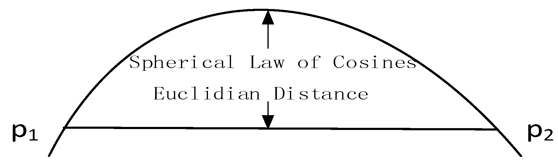
An occupied trip is a sequence of GPS points of a taxi trajectory. P = {p1, p2, …, pn}, where n ≥ 5, and the car status of p1 > pn is 3. In order to calculate the distance of an occupied trip, we need to calculate the geographical distance of the origin (p1) and destination point (pn) of the occupied trip. To this end, there are two popular methods that can be used: Euclidian distance approximation and the spherical law of cosines [21]. The difference between the two methods is explained by Figure 2.
According to the Euclidian distance, the distance between two points p1 and p2 would be equal to the cord p1→p2, whereas the actual distance would be along the circular arc p1→p2 as in the spherical law of cosines [22]. In this study, we used the spherical law of cosines to calculate the geographical distance (by kilometers) of an occupied trip as follows.
where lat1, lat2, log1 and log2 are the latitude and longitude of points p1 and p2, respectively. R is the radius of Earth (6371 km). Then, the total distance of an occupied trip OT is calculated by the summation of the distance between the pair of GPS points of the OT’s trajectory using Formula (1). Then, the total driving distance (by kilometers) of a taxi (x) in 61 days would be calculated as follows:
where n represents the total days (61 days), whereas m is the total occupied trips of a taxi x in a day i.
Then, the fare of an occupied trip can be calculated using the following formula.
• Duration:
The duration of an occupied trip can be simply obtained by the following formula:
where Timeend and Timebegin are the beginning and the end time of an occupied trip. Then, the total driving duration (by minutes) of a taxi (x) in 61 days would be calculated as follows:
where n represents total days (61 days), whereas m is the total occupied trips of a taxi x in a day i.
• Income:
After obtaining the duration and the distance of occupied trips, the fare of an occupied trip is calculated as in Formula (5).
where d is the distance of the occupied trip as Formula (1) and P0, P2, P7 and FS are standard fares according to the taxis’ fare system in Wuhan City (in 2013), as in Table 3.
Examples of occupied trips’ information extracted from raw GPS data are presented in Table 4.
Then, the total income of a taxi (x) would be calculated as follows:
where F(di) is the income of a trip i calculated as Formula (5), m is total occupied trips in a day i of a taxi x and n is the total days (61 days).
• Driving profitability:
As mentioned, in this study, the driving profitability of each taxi driver is considered by three features, total distance, total duration and total income, as follows.
Cluster analysis is a valid method for classifying driving profit of taxi drivers into different groups. In this study, the K-means cluster method, which is used widely for cluster analysis in datamining, is employed to classify the drivers into different groups based on the proposed features X. Using a pre-determined number of clusters, the K-means cluster method partitions the driving profitability features X into k clusters, where each driving profitability belongs to a cluster whose mean is closest to its value. The K-means method minimizes the within-cluster sum of squares:
where X = (X1, X2, X3, . . ., Xn) is the set of obtained data, which represents the feature X1 (DistanceTotal, DurationTotal, IncomeTotal) in the context of this paper; S = (S1, S2, S3, . . ., Sn) represents the set of k clusters; and i denotes the mean center of a cluster set Si.
In this study, the predefined K-value of K-means clustering would be set to 3, and then, the cluster results would be grouped into three profitability levels, high, moderate and low.
Due to the huge volume of taxi drivers in the dataset (6480 drivers), the three driving profitability levels would be represented by randomly selecting 20% of each clustering group. For instance, 20% of high profitability group would be selected to represent the high profitability level, and so on.
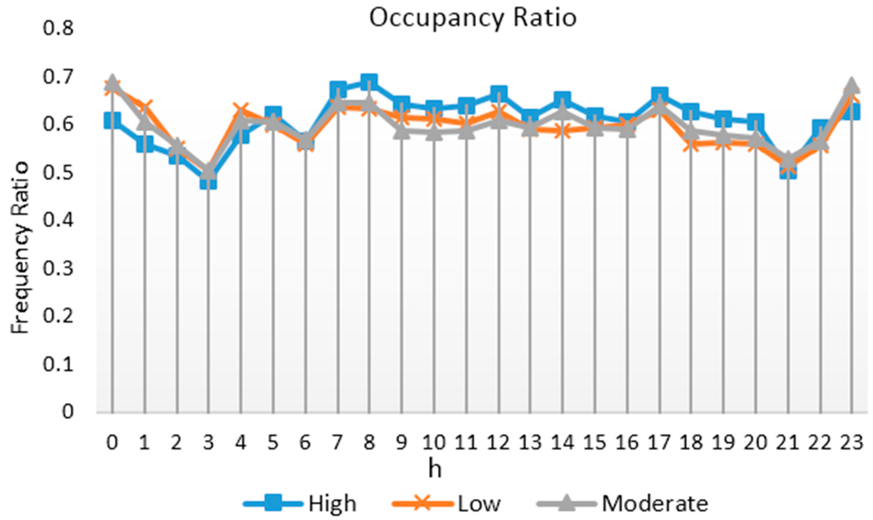
In addition, the occupancy ratio of the three levels’ is calculated by capturing and comparing the distance of the occupied and vacant trips using Formula (9):
The occupancy ratio can provide knowledge of the proportion of the distance of occupied trips to the total distance cruised in the whole working duration. The comparison among the three driving profitability levels of the driver related to peak and off-peak duration will be shown a time graph followed by explanations.
2.2.2. A Method for Extracting Cruising Trips and Stopping Spots
This study focuses on investigating the temporal and spatial patterns of taxis’ vacant trips. Based on the taxis’ trajectory and trips, vacant trips can be divided into two types, stopping spots and cruising trips.
• Stopping spots:
In this study, a stopping spot can be represented by a location where a sequence of five continuous GPS points occur and last more than 3 min, whereas the case when a taxi is moving without a passenger is called a cruising trip. There is a need to detect stopping spots and cruising trips in order to explore their driver behavior patterns. The following is a method for detecting stopping spots, (1) vacant trips, i.e., trips whose GPS records have a car status equals to 1, were extracted, (2) sequences of static GPS points of vacant trips, i.e., more than 5 continuous GPS points with a velocity of zero, were isolated and the beginning and ending time, location and duration for each sequence recorded, (3) the mean center of each sequence is obtained using longitude and latitude, and this center is considered as a stopping spot.
In general, each detected stopping spot is associated with temporal attributes (e.g., stopping duration, beginning and ending timestamp). For different purposes of these trips, some of those long trips may refer to locations with different meanings, such as parking lots, railway stations or hotels or even traffic congestion locations at road segments and intersections.
• Cruising trips:
After detecting stopping spots, cruising trips were obtained by removing the records of stopping spots from vacant trips. Cruising trips contain many attributes such as starting and ending location (i.e., longitude and latitude), starting and ending time slot, duration, taxi ID, etc. These attributes can assist in investigating the patterns of taxi drivers.
2.2.3. Mobility Patterns of Cruising Trips and Stopping Spots
Once a taxi driver drops off a passenger and begins cruising city roads, he or she plans to reduce cruising duration and rapidly picks up a new passenger. In addition, when a taxi driver stops the taxi for a long time, he/she may miss opportunities to pick up a new passenger and to increase his/her profitability. Then, there is a demand to reveal the different mobility patterns of the taxi drivers categorized by profitability levels through studying cruising trips and stopping spots extracted from their daily trajectory traces.
• Mobility patterns of cruising trips:
Unlike the case in occupied trips, in cruising trips, taxi drivers can select and cruise in the way they want in order to save oil and to quickly pick up a new passenger. Therefore, investigating taxi drivers’ trajectory traces may provide some details to understand the mobility patterns of taxi drivers. In order to investigate their mobility patterns, temporal and spatial patterns of the three profitability levels of drivers are investigated.
In the temporal patterns, the cruising time of taxis until picking up new passengers is considered, and then, the variation of the frequency and the cumulative distribution of the three profitability levels of drivers will be shown in a time graph. Cruising time is divided into time intervals between 0 and 60 min, and the frequency of cruising trips would then be determined with these intervals. Finally, the results would interpret the differences of the cruising time distribution of the drivers categorized by profitability levels.
In the spatial patterns, a map matching method is applied by loading starting and ending coordinates (longitude and latitude) of cruising trips on the Wuhan map using fish net and polygon maps in the ArcGIS (version 10.2) software
After performing the dataset’s spatial examination, we found that the main area of taxis’ trajectories and trips were in the area with the geographical coordinates longitude (113.920, 114.639), latitude (30.300, 30.899). Therefore, Wuhan map was split into 69 × 67 square grid cells. Each grid cell was given a number between 1 and 4623 and has four dimensions according to the split coordinates. For instance, grid cell No. 1 has four dimensions: (longitude (113.920, 113.930), latitude (30.300, 30.308)). The geographical coordinates of cruising trips were matched with dimensions of grid cells in order to obtain the density of the spatial distribution of cruising trips. Later, these grid cells are combined and joined with the corresponding Wuhan City fishnet and polygon maps. In the end, the results on Wuhan City’s map are interpreted and explained in detail.
• Mobility patterns of the stopping spots of three profitability levels:
In order to understand drivers’ behavior (human mobility) and their impact on daily income, there is a need to investigate the spatial and temporal patterns of stopping spots. To this end, firstly, the general temporal distribution of stationary spots is studied. Secondly, the spatial and temporal patterns of long stopping spots are investigated. Finally, the spatial and temporal patterns of stopping spots on the off-peak duration derived from the occupancy ratio are explored.
(a) General temporal distribution:
In order to understand the wide-ranging temporal distribution of stopping spots, we calculated the hourly average waiting duration of stopping spots of the drivers by three profitability levels within 61 days. A time line graph that shows the variation of the average hourly stopping duration of the three levels is drawn and followed by explanations.
(b) Spatial and temporal patterns of stopping spots in longer durations by DBSCAN:
The long waiting time at stopping spots may reflect either long parking or long waiting on streets. Long parking may imply sleeping at nights or resting at daytime, whereas long waiting on streets may represent traffic congestion.
Once a taxi driver, without a passenger, waits or stops at a location for a long time, this may influence the overall daily income. Therefore, this section presents an investigation of the spatial and temporal distribution of stationary spots on relatively long durations.
The stopping spots of the three profitability levels of drivers, in Section 2.2.1, with a waiting duration of more than 25 min would be extracted and collected. A modified density-based spatial clustering of the applications with the noise DBSCAN algorithm is applied to cluster these stopping spots based on their density.
Firstly, we provide an introduction to the DBSCAN algorithm. Secondly, we describe the implementation of the DBSCAN algorithm on stopping spots of longer durations.
(b.1) Density-based spatial clustering DBSCAN:
DBSCAN, a density-based clustering algorithm, is developed to discover clusters in arbitrary shapes. The key feature of DBSCAN is that it confines the minimum number of objects in a given radius of each cluster. In addition, DBSCAN shields the interference of noisy data effectively.
In order to make use of the DBSCAN algorithm, this study considers the following: (1) measuring the distance between two data points (stopping spots’ locations) using the spherical law of cosines method as in Formula (1); and (2) determining the centers of clusters by calculating the average of the latitudes and longitudes of all of the data points in each cluster by Formula (10).
where are n points included in a cluster and and refer to the latitude and longitude of a point , respectively. The DBSCAN algorithm used in our study is described as shown in Algorithm 1.
| Algorithm 1: DBSCAN algorithm in our study. |
| Input: points (stopping spots), EPS, MinPts |
| Output: clusters set C |
| 1: C = null; 2: for each unvisited point p in points 3: mark p as visited; 4: obtain p’s EPSNeighborhood within EPS using spherical law of cosines method as in Formula (1); 5: if | p’s EPSNeighborhood|< MinPts, then mark p as a noise point; 6: else set C as a new cluster and add p to cluster C; 7: for each point q in p’s EPSNeighborhood 8: if q unvisited, mark q as visited obtain q’s EPSNeighborhood by EPS similar to Step 4; 9: if |q’s NeighborPts| ≥ MinPts 10: p’s EPSNeighborhood = p’s EPSNeighborhood joined with q’s EPSNeighborhood 11: end if 12: end if 13: if q is not yet member of any cluster, then add q to cluster C; 14: end if 15: end for 16: end if 17: obtain the cluster center of C using Formula (10) 18: end for |
The DBSCAN algorithm in this study will be explained as follows: Firstly, an unchecked point p is selected, and the size of p’s EPSNeighborhood is compared with the predefined MinPts (the reason for selecting the optimal values of EPS and MinPts will be explained in the Discussion section). If p’s EPSNeighborhood is less than MinPts, p would be considered as a noise point; otherwise, a new cluster C would be set, and all p’s EPSNeighborhood would be added into a new cluster C. Secondly, the algorithm would check the points in EPSNeighborhood the same as in Step 4. Thirdly, the algorithm would compare the number of q’s EPSNeighborhood with MinPts and join q’s EPSNeighborhood with p’s EPSNeighborhood. Finally, the algorithm results in all clusters along with their cluster centers.
(b.2) Spatial and temporal patterns of stopping spots for longer durations by DBSCAN:
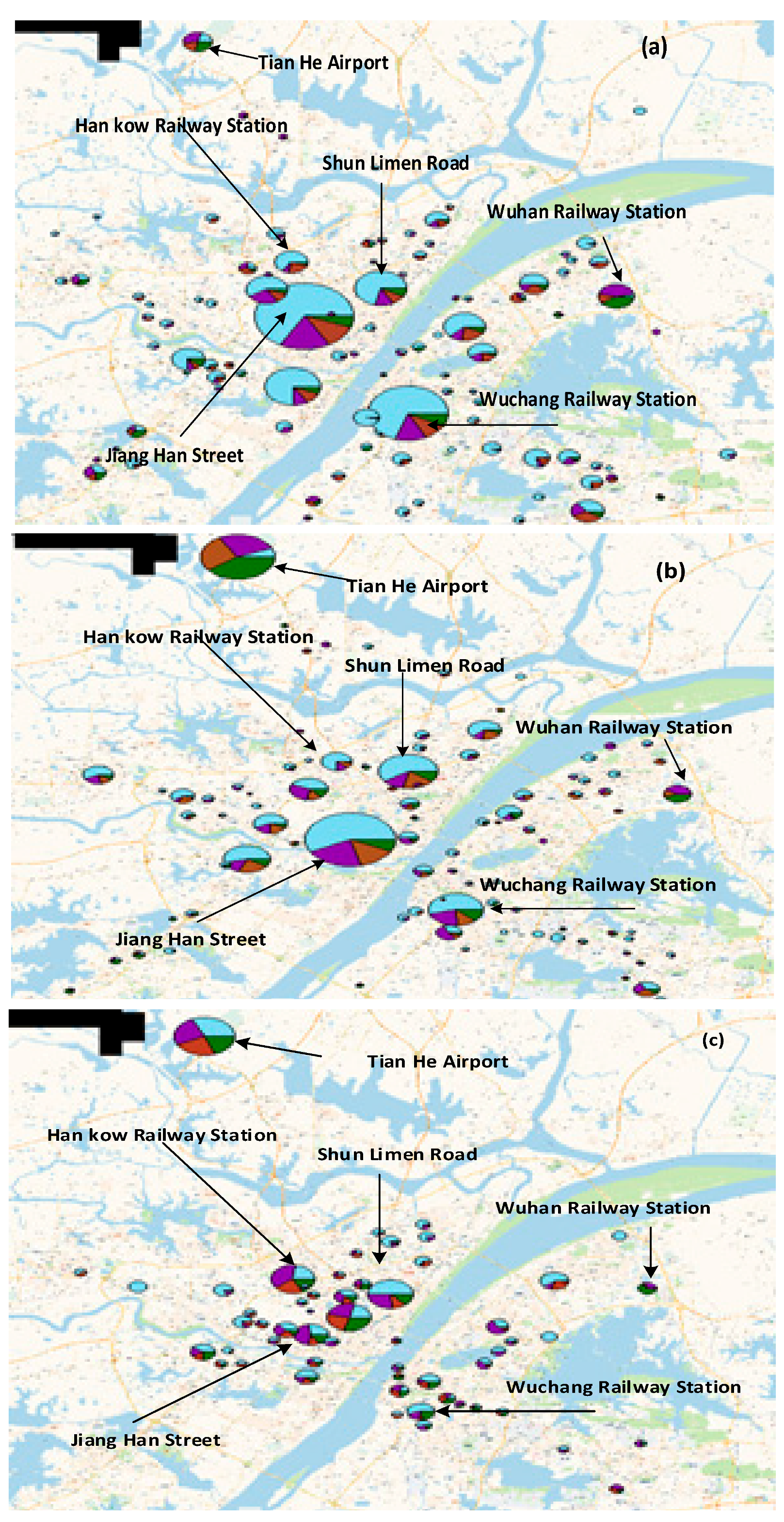
After implementing the DBSCAN algorithm, we may obtain many clusters as a result. In order to better understand the spatial and temporal distribution of the obtained clusters, the duration of each day was divided into four time intervals, namely midnight (12 a.m.–6 a.m.), morning (6 a.m.–12 p.m.), afternoon (12 p.m.–18 p.m.) and evening (18 p.m.–12 a.m.); then, the whole number of elements was calculated for each cluster in each time interval.
Pie chart (circular chart divided into sections) graphs in the ArcGIS software were used to illustrate and visualize the spatial and temporal distribution of the obtained clusters. The spatial location of each pie chart represents the center of the corresponding cluster, and the size of each pie chart is proportional to the total number of elements in corresponding cluster. Each pie chart was divided into four colored sectors with four colors (i.e., light blue, purple, green and brown) corresponding to the four time intervals. These sectors are proportionally sized to a corresponding number of the cluster elements in each time interval.
(c) Human mobility of stopping spots in off-peak duration:
There is a variation of the occupancy ratios’ distribution among the three profitability levels of drivers. This variation, which might be caused by distinct driving behaviors of taxi drivers, may lead to a difference in the overall income of the taxi driver. Therefore, there is a need to investigate the spatial and temporal distribution of stopping spots in this duration.
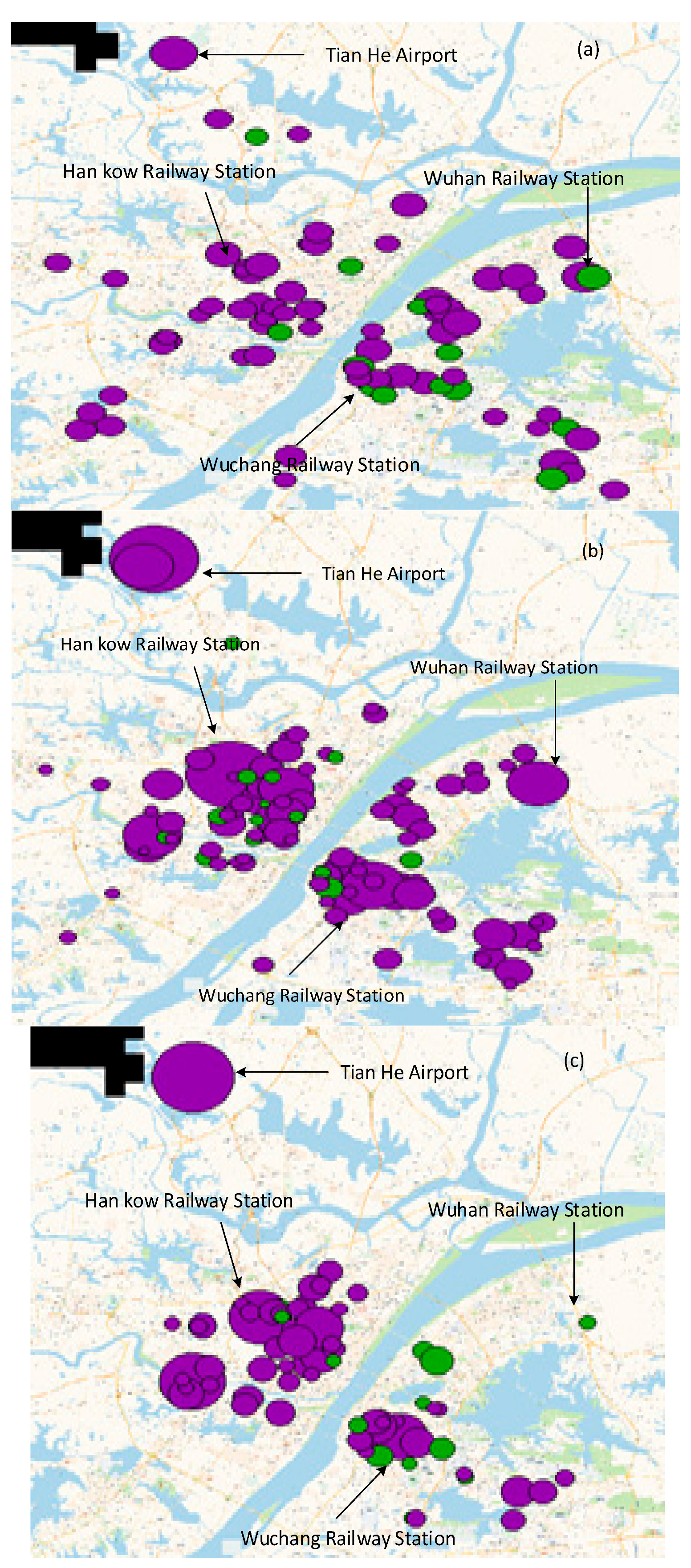
To end this, we detect the off-peak duration, which represents a duration with a lesser occupancy ratio of the three levels of drivers between two high peak durations. Then, the DBSCAN method was used to form clusters using stopping trips in the off-peak duration, and each cluster can either be a parking spot or a traffic congestion spot. The distance between stopping spots in each cluster and the nearest large street would be calculated and compared with the pre-defined threshold as follows: traffic congestion spot (<50 meters) and a parking spot (≥50 meters). If more than 50% of stopping spots in a cluster are traffic congestion spots, this cluster can be considered as a traffic congestion cluster; otherwise, the cluster can be considered as a parking spot cluster. Finally, we can derive a comparison of the average duration of traffic congestion and parking locations, and then, we would explain the meaning of these results.
3. Results
3.1. Classification and Occupancy Ratio of Taxi Drivers with Three Driving Profitability Groups
After implementing the K-means clustering method, taxi drivers are categorized into three groups according to their profitability, namely low profitability group, moderate profitability group and high profitability group. The output of the cluster analysis is shown in Figure 3, and Table 5 summarizes the statistical characteristics of the three driving profitability groups.
The distribution of taxi drivers shows that the low profitability group has the minimum drivers, whereas the moderate profitability group has the maximum number of drivers. We can observe that the distance and income of the high profitability group are more than three-times those of the low profitability group, and the duration of the moderate and high profitably groups is much higher than that of the low profitably group, which makes the cluster result reasonable. This result may be caused by different daily mobility of taxi drivers.
As the volume of the dataset is huge and in order to obtain obvious results, the volume of the dataset of our study is reduced. The three profitability levels of drivers are represented by selected samples from profitability groups as follows: each of the three profitability levels is represented by a sample of 200 drivers, which are randomly selected from their corresponding profitability groups. For instance, 200 drivers randomly selected from the high profitability group would present the high profitability level.
In addition, the occupancy ratio of the three driving profitability levels was calculated by capturing and comparing the distance of the occupied and vacant trips using Formula (4). Figure 4 depicts the occupied ratios of high, moderate and low profitability drivers during 61 days.
Obviously, the occupied ratio of the three profitability drivers’ has several peaks (e.g., at 4 a.m., 2 p.m. and 5 p.m.) and valleys (e.g., at 3 a.m., 6 a.m. and 9 p.m.). In addition, high profitability drivers generally have a much higher occupancy ratio. Except the area between 9 a.m. and 11 p.m., the differences of the occupancy ratio among high, moderate and low profitability drivers are much smaller than those in other time slots. Later, this duration, which is located between two peak durations, can be investigated to understand the reasons behind the difference of the occupancy ratio.
3.2. Extracting Cruising Trips and Stopping Spots of Three Profitability Levels
This study focuses on investigating the temporal and spatial patterns of taxis’ vacant trips. As mentioned above, vacant trips can be divided into two types, stopping spots and cruising trips.
As shown in Table 6, the three profitability levels of drivers have different volumes of the three trip types. High profitability drivers are at the top of the total number of occupied and stopping spots that may be interpreted as they are eager to earn money and save oil; however, they cruise less than moderate profitability drivers. The low profitability drivers have the lowest occupancy, cruising and stopping volume of trips, which may be caused by less experience or not knowing the city roads very well. Although cruising trips are the highest in the moderate profitability drivers, the occupied and stopping spots results are near the high profitability numbers.
3.3. Spatial and Temporal Patterns of Cruising Trips
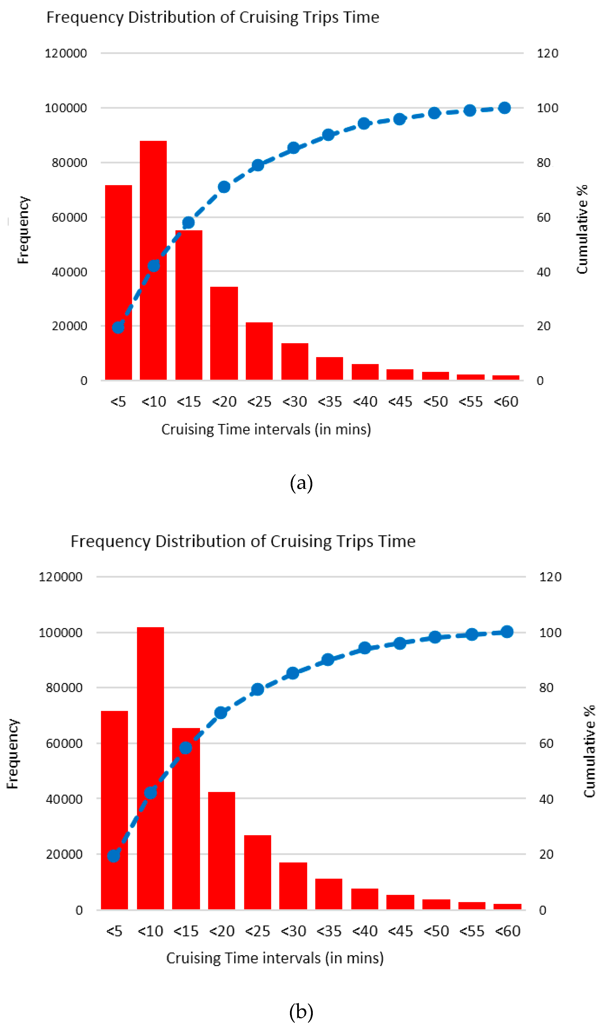
The results of spatial and temporal patterns are derived and interpreted as follows. In the temporal patterns, we studied the frequency distribution of the time intervals of cruising trips. The duration of the cruising trips of the three were calculated, and the results are shown as in Figure 5.
As Figure 5a–c shows, 60% and 83% of the cruising time of high profitability level drivers can be reached in less than 10 and 20 min, respectively. In other words, 83% of the cruising time of high profitability level drivers is less than 20 min before picking up a new passenger, and that is a good index. Besides, unlike high profitability level drivers, both medium and low profitability level drivers show that 42% and 79% of the cruising time is in less than 25 min, and that may lead to increased oil consumption and then reduced daily income.
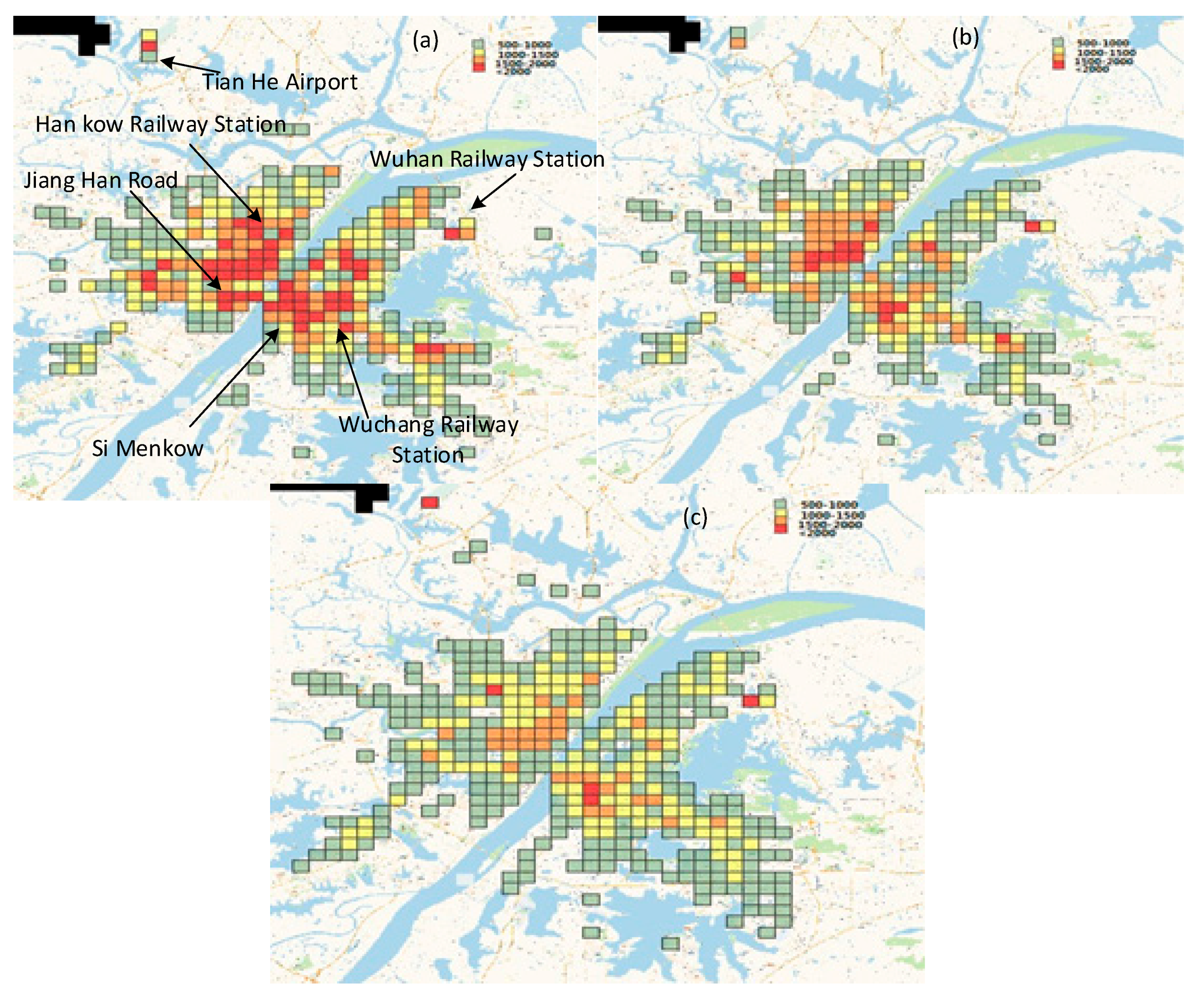
The starting and ending coordinates of the cruising trips are uploaded and matched with gird cells, and the results are shown in Figure 6.
From Figure 6, it is obvious that the three profitability levels of drivers present different spatial distributions of cruising trips. High profitability drivers have more grid cells with high density (red) focused on the main crowded locations, such as Wuchang and Han Kou Railway Station, Jiang Han Street and Si Menkou. Unlike the case for high profitability drivers, grid cells for low profitability drivers have less density (green and yellow) and concentrate on further locations. Moderate profitability drivers present grid cells with a density greater than in the low profitability drivers and share the crowded locations as the low profitability drivers.
The results above can be interpreted as follows: the spatial distribution of the low and relatively moderate profitability drivers is more dispersed and shows more concentration on cruising further away from the main economic locations in the city, and this may relate to driver experience. As shown in Figure 6a, the high profitability drivers may drive around the city center and may know that crowded places such as railway stations and main roads in specific times are good opportunities for getting new passengers, then they cruise depending on their knowledge. This may impact their whole income and oil consumption. On the other side, and as shown in Figure 6c, low profitability drivers drive to further places, and this may occur due to the lack of experience or due to not knowing city roads well.
3.4. Spatial and Temporal Patterns of Stopping Spots with Three Profitability Levels
3.4.1. General Temporal Patterns
As shown in Figure 7, high profitability drivers wait less time (average of 21 min) than moderate and low profitability drivers (average of 31 and 43 min, respectively). Moreover, the figure shows a high peak during dawn hours (2 a.m.–6 a.m.), and low profitability drivers reached 105 min at 3 a.m.; this might be interpreted as sleeping time. In general, low profitability drivers wait a longer time, followed by moderate drivers; this may relate to driving experience and driving years.
3.4.2. Spatial and Temporal Patterns of Stopping Spots of Longer Durations
In implementation clustering analysis, the selected values of two parameters (EPS and MinPts) of DBSCAN affect the accuracy of the clustering results. This study found that the optimal results of clustering can be obtained with the optimal distance (Eps = 20 meters) and minimum points (MinPts = 10 points).
The implementation of the DBSCAN method on stopping spots of longer durations produced 102, 109 and 59 clusters for high, moderate and low profitability drivers, respectively. Figure 8a,b,c shows the spatial and temporal patterns of the stopping spots of high, moderate and low profitability drivers, respectively, of a longer duration (more than 25 min).
In general, the local airport and the three train stations of Wuhan City are the locations that have relatively large pie charts in Figure 8, and the pie charts have large proportions at midnight and in the mornings. This leads to a derivation that the three profitability levels of drivers often prefer waiting at these locations at these time intervals. However, there are observed variations of the spatial and temporal distribution.
As shown in Figure 8a, pie charts for low profitability drivers are small and few, and concentrated in Han Kou district, and there is a big pie chart for Tian He airport. According to the various colors on the charts, the four time intervals are distributed on the duration time. This may be interpreted as there is no regular time for the stopping time, and drivers stop long durations in all time intervals.
Figure 8a,b shows the long duration of high and moderate profitability drivers. In terms of high profitability drivers, large charts are located at the three train stations, Shun limen and Jiang Han Street. In addition, the charts are light blue and purple, corresponding to the midnight and morning, respectively. This can be interpreted as the drivers prefer to take their long-breaks in time periods when passengers are too few, and this reduces oil consumption and impacts the total income. The spatial and temporal distribution of moderate profitability drivers is relatively similar to high profitability drivers with some differences, such as a smaller size of charts, and the time intervals are mainly distributed on mornings and midnights. This mean that moderate profitability drivers perform better than low profitability drivers.
3.4.3. Spatial and Temporal Patterns of Stopping Spots in Off-Peak Duration
In Figure 4, there is a significant variation of the occupancy ratios’ distribution among the three profitability drivers, especially from 9 a.m.–11 a.m. After implementing the method in Section 2.2.3, we used the pie chart graph to visualize the finding of traffic congestion and parking clusters as shown in Figure 9.
As shown in Figure 9, colored pie charts represent the traffic congestion and parking clusters, where green pie charts represent congestions clusters, whereas purple pie charts are parking clusters. The size of each pie chart is proportional to the total number of elements in the cluster. Although most pie charts in the figure represent parking spots and very few pie chart represent congestion, there are some distinct features between the three types of profitability levels of drivers.
As shown in Figure 9b, moderate profitability drivers have a greater number and a larger size of scattered parking and congestion clusters than for the high and low profitability drivers. This may mean that the group may be parking or be in traffic congestion compared to the other groups, and this may lead to a low occupancy ratio, as shown in Figure 4. In terms of high profitability drivers in Figure 9a, parking and congestion clusters are less and smaller in size, and this may mean that they pick up more passengers in this time interval, then leading to the increased occupancy ratio. The low profitability drivers, as shown in Figure 9c, have a relatively greater number of congestion and parking clusters, more than the high profitability drivers, and this may be interpreted as more parking and congestion frequency from 9 a.m.–11 a.m. Besides, Figure 9b,c shows that parking clusters for moderate and low profitability drivers are bigger especially in crowded locations, such as the airport and railway stations. This may occur due to drivers preferring to wait there rather than cruising, and this may influence their daily income.
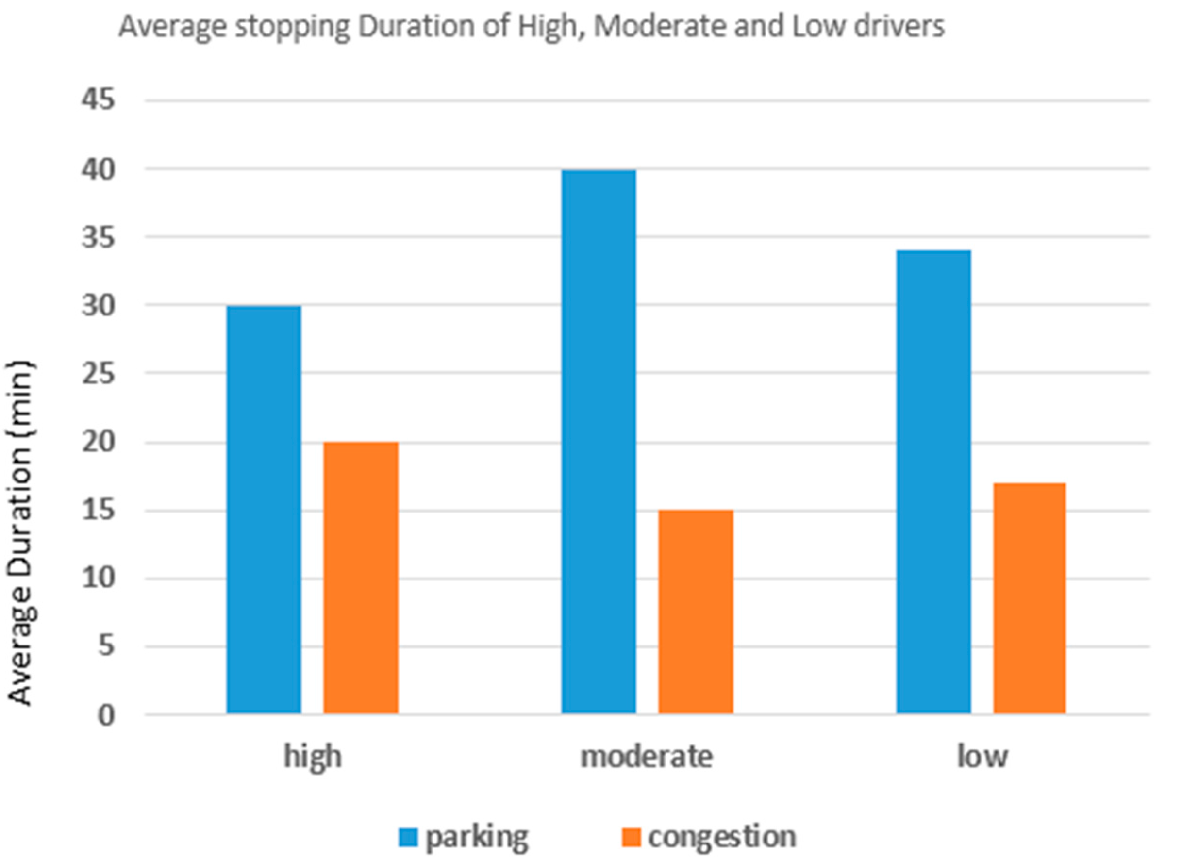
Figure 10 shows the average stopping duration (in minutes) spent on traffic congestions and parking spots for high, moderate and low profitability drivers. The average duration spent on traffic congestion is less than for parking spots in the off-peak duration. Moderate profitability drivers wait longer in parking spots than other drivers, whereas high profitability drivers wait the longest time for traffic congestion among the other two driver groups.
4. Discussion
This section contains two parts: a discussion of the findings and linking them to provide a comprehensive view of the results, followed by a comparison between the proposed method and other similar studies.
4.1. Discussion of the Findings
The sections above investigated in detail the mobility patterns (spatial-temporal distribution of the trajectory traces) of high, moderate and low profitability taxi drivers, which reflect their distinctive driving behaviors. In this section, we try to link the derived results together and to provide a comprehensive analysis and discussion of the findings of the mobility patterns of taxi drivers.
There is an observed variation of the overall temporal patterns of taxi drivers during their cruising trips and stopping spots. As shown in Figure 4, the line chart graph, which represents the variation of the occupancy ratio of high, moderate and low profitability drivers, the high profitability drivers’ drive longer distances (especially in the daytime) with passengers than others. In addition, in terms of cruising trips’ durations, high profitability level drivers normally drive more cruising trips than low profitability level drivers (see Table 6), but cruise less in duration (80% within 20 mins) compared to moderate and low profitability levels (80% within 30 and 35 min, respectively) (see Figure 5). These variation results may reduce the daily profit by increasing oil consumption. In terms of the durations’ distribution for stopping spots, high profitability taxi drivers have constantly shorter average durations (see Figure 7), better than other drivers, which may in turn compensate the loss of the longer cruising frequency and increase their profitability, as well.
In terms of the spatial cruising distribution, various spatial patterns are discovered. The spatial distribution of the high profitability level drivers is more compact and concentrated in main economic locations of Wuhan City, as shown in Figure 6a. Unlike for high profitability drivers, the spatial distribution of the moderate and low profitability drivers is more dispersed and shows a greater concentration on cruising further away from the main economic locations in the city. This may impact their overall income, as they surely consume more oil.
In addition, comparing the spatial distribution of cruising trips with the spatial distribution of long stopping spots, we found that there is an inverse correlation between cruising spatial distribution and the long-stopping spot around midnight with high and moderate profitability drivers, which in turn may reveal that these drivers might not prefer cruising around their long stop trips or parking locations.
There are variances of the mobility patterns of drivers’ stopping spots. The results provided from Figure 4 show occupancy ratios of high, moderate and low profitability drivers; there is an observed variation within off-peak hours, which might lead to the reasons behind drivers’ profitability variances. Therefore, a study was conducted to reveal spatial and temporal patterns in the off-peak duration, from 9 a.m.–11 a.m. The finding results showed that the high, moderate and low drivers spend relatively similar average time on street congestion, although high profitability drivers spend more time than other groups, but there is an observed distinction of average time for parking places (see Figure 10). One reason might be considered, that low and moderate drivers wait considerably longer at some locations in the city; Figure 9 shows that there are big waiting areas at Tian He Airport and Han Kou Railway Station for both moderate and low profitability drivers.
To sum up, the results show that the daily behavior of taxi drivers has a significant impact on their profitability. The mobility patterns of drivers lead to different spatial and temporal patterns on cruising trips and stopping spots. This may occur for different reasons, such as driver experience, awareness of city roads and other reasons.
4.2. Comparison with Similar Studies
In this study, we considered the case that normally there are at least two taxi drivers that drive the same car, and then, there is a need to firstly detect the drivers according to their shifts and then investigate the impact of driving behavior instead of ignoring this important point, as in the works in [10,11], and which may obtain inaccurate results.
Comparing to the works in [10,11], our proposed approach divided the drivers into three groups based on three features, namely distance, duration and income. Dividing taxi drivers into three groups can provide a comprehensive view of the variety of drivers and then can provide us a deep insight into the impact of their driving behavior on profitability.
Instead of dividing taxi drivers using only income ranking in [10,11], our study adopted a novel method by the K-means clustering technique to divide drivers based on three profitability features, namely distance, duration and income. Hence, the findings may present a powerful basis of the following steps by providing an accurate grouping of taxi drivers.
Unlike in [11], which calculated the mean center of cruising trips for showing the distribution of cruising trips’ locations, our study adopted a grid map method for grouping pick-up and drop-off points of cruising on the map of Wuhan City, which shows a reasonable distribution and better understanding of cruising trips’ locations.
During the implementation of the approach, we found that the selection of the values of two global parameters (Eps and MinPts) in DBSCAN affects the accuracy of clustering results. We then discuss the effects of the two parameters, without providing figures due to the page limitations, as follows:
Firstly, we describe the effect of parameter MinPts by using the data of high profitability drivers in the period of 22:00–6:00 in September and October 2013; we can get the result of 70 clusters (Eps = 10, MinPt = 15) and 40 clusters (Eps = 10, MinPts = 5). The view of the results shows that the bigger the MinPts value is, the less the number of cluster would be. Therefore, after determining the appropriate value of Eps, the bigger value of MinPts (about 20), which indicates the stopping spots’ information in a macroscopic view, is a fine choice if considering the transportation status at night. Furthermore, the smaller value of MinPts, which indicates the detailed and accurate stopping spots’ information, is beneficial to the optimization of key points.
Secondly, we describe the effect of parameter Eps. By using the data of high profitability drivers in the period of 22:00–6:00 in September and October 2013, the clustering results show around 102 clusters (Eps = 30, MinPt = 20) and 59 clusters (Eps = 10, MinPts = 20). The findings show that after setting the appropriate value of MinPts, the proper value of Eps is a fine choice if considering the transportation status at nights in the area with proper density. As for a dense area, the smaller value of Eps would be a fine choice.
5. Conclusions
This paper investigates and analyzes the impact of drivers’ behavior patterns on taxi drivers’ profitability using taxi GPS data. Specifically, the spatial and temporal patterns, of vacant trips, were studied in order to reveal their impact on taxi drivers’ profitability. The analysis of the study is general and can be implemented in any area. With respect to the availability of dataset, taxi GPS data of Wuhan City have been used as an example for implementing the proposed approach.
Firstly, using the K-means clustering method, three driver groups were detected based on three features affecting driving profitability derived from daily occupied trips for two continuous months (September and October 2013). Secondly, cruising trips and stopping spots were extracted from unoccupied trips. Thirdly, a comparison of the profitability levels of drivers in terms of spatial and temporal patterns on cruising trips and stopping spots is provided. To understand the human mobility of cruising trips in terms of the three profitability drivers, we calculated and compared the frequency distribution during time intervals to represent their differences. In addition, a map matching method and grid cell-based density method were applied to draw and present the spatial distribution of cruising trips.
For stopping spots, we studied the general temporal patterns of stopping spots by comparing the average waiting duration of the three profitability groups of drivers within two months. A DBSCAN clustering method was adopted to investigate the spatial and temporal patterns of long stopping spots, and the obtained clusters were matched to the map of Wuhan City. Spatial and temporal patterns of stopping spots in off-peak duration were investigated. Parking spots and traffic congestion spots were distinguished and presented using pie chart graphs and time graphs.
The results of this study present evidence of the fact that there are obvious driving behavior differences for high, moderate and low profitability drivers. As a case study of Wuhan City, we found that high profitability drivers usually have high frequency cruising trips compared to low profitability level drivers, but cruise lesser durations compared to moderate and low profitability drivers. Cruising trips of high profitability drivers were concentrated in crowded locations, while they were dispersed in moderate and low drivers.
In addition, once we compared the spatial distribution of cruising trips with the spatial distribution of long stopping spots, we found that there is an inverse correlation between cruising spatial distribution and the long-stopping spot around midnight with high and moderate profitability drivers, which in turn may reveal that these drivers might not prefer cruising around their long stopping trips or parking locations. There are many reasons for these results, such as driver experience, awareness of city roads and other reasons. This study may provide suggestions and insights for taxi companies and taxi drivers in order to increase their profit and to enhance the efficiency of the taxi industry.
In the future, we plan to broaden and deepen this study in two directions. First, we may integrate more effective parameters, such as weather, road environment and driving years, in order to provide a richer picture of the human mobility of taxi drivers. Second, we would analyze a larger dataset and develop a taxi recommender system using a mobile phone device.
Acknowledgments
This paper is supported by the National Nature Science Foundation of China (Analysis of Time-Based Fatigue Level Prediction Model for Full Driving Cycle Considering the Effect of Circadian Rhythm and Driving Workload), National Key Projects in Science & Technology of China (2014BAG01B03, 2014BAG01B05), the Academic Leader Project of Wuhan (2012711304457) and the Fundamental Research Funds for the Central Universities (WUT: 2014-IV-137).
Author Contributions
Hasan.A.H. Naji initiated the idea of the study, designed the research scheme and methods and wrote the manuscript. Chaozhong Wu provided the dataset and supervised the instructions during the implementation. Hui Zhang helped with writing and providing advice in the study. All of the authors have read and approved the final manuscript.
Conflicts of Interest
The authors declare no conflict of interest.
References
- Wuhan Transportation Development Strategy Research. 2013 Wuhan Transportation Development Annual Report. Available online: http://www.wpl.gov.cn/pc-1516-51822.html. (accessed on 15 June 2016).
- Yuan, J.; Zhang, Y.; Zhang, L.H.; Xie, X.; Sun, G.Z. Where to find my next passenger. In Proceedings of the 17th ACM SIGKDD International Conference on Knowledge Discovery and Data Mining, San Diego, CA, USA, 21–24 August 2011; pp. 109–118. [Google Scholar]
- Occupational Employment Statistics. Occupational Employment and Wages. Taxi Drivers and Chauffeurs. Available online: http://www.bls.gov/oes/current/oes533041.htm#(2) (accessed on 3 Septmber 2016).
- Driven Into Poverty A Comprehensive Study of the Chicago Taxicab Industry. Available online: https://ler.illinois.edu/wp-content/uploads/2015/01/Taxi-Income-Report-Final-Copy1.pdf (accessed on 15 December 2016).
- Liang, L.; Andris, C.; Biderman, A.; Ratti, C. Revealing taxi drivers mobility intelligence through his trace. In Movement-Aware Applications for Sustainable Mobility: Technologies and Approaches; Information Science Reference: New York, NY, USA, 2010; pp. 105–120. [Google Scholar]
- Xu, T.; Zhu, H.S.; Zhao, X.Y.; Liu, Q.; Zhong, H. Taxi Driving Behaviour Analysis in Latent Vehicle-to-Vehicle Networks: A Social Influence Perspective. In Proceedings of the 22nd ACM SIGKDD International Conference on Knowledge Discovery and Data Mining, San Francisco, CA, USA, 13–17 August 2016; pp. 1285–1294. [Google Scholar]
- Yang, W.X.; Wang, X.; Rahimi, S.M.; Luo, J. Recommending Profitable Taxi Travel Routes Based on Big Taxi Trajectories Data. In Proceedings of the Pacific-Asia Conference on Knowledge Discovery and Data Mining, Minh City, Vietnam, 19–22 May 2015; pp. 370–382. [Google Scholar]
- Powell, J.W.; Huang, Y.; Bastani, F.; Ji, M. Towards reducing taxicab cruising time using spatio-temporal profitability maps. In Proceedings of the 12th International Symp. Spatial Temporal Databases, Minneapolis, MN, USA, 24–26 August 2011; pp. 242–260. [Google Scholar]
- Gao, Y.; Xu, P.P.; Lu, L.; Liu, H.; Liu, S.Y.; Qu, H.M. Visualization of Taxi Drivers' Income and Mobility Intelligence. In Proceedings of the 2012 International Symposium on Visual Computing (ISVC), Rethymnon, Greece, 16–18 July 2012; pp. 275–284. [Google Scholar]
- Zhu, B.; Xu, X. Urban Principal Traffic Flow Analysis Based on Taxi Trajectories Mining. In Advances in Swarm and Computational Intelligence; Springer: New York, NY, USA, 2015; pp. 172–181. [Google Scholar]
- Ding, L.F.; Fan, H.C.; Meng, L.Q. Understanding Taxi Driving Behaviours from Movement Data. In Agile; Springer: New York, NY, USA, 2015; pp. 219–234. [Google Scholar]
- Ding, L.F.; Yang, J.; Meng, L.Q. Visual Analytics for Understanding Traffic Flows of Transport Hubs from Movement Data. In Proceedings of the International Cartographic Conference, Rio de Janeiro, Brazil, 19–21 August 2015; pp. 23–28. [Google Scholar]
- Kumar, D.; Wu, H.Y.; Lu, Y.; Krishnaswamy, S.; Palaniswami, M. Understanding Urban Mobility via Taxi Trip Clustering. In Proceedings of the 17th IEEE International Conference on Mobile Data Management (MDM), Porto, Portugal, 13–16 June 2016; pp. 318–324. [Google Scholar]
- Chen, C.; Zhang, D.Q.; Li, N.; Zhou, Z.H. B-Planner: Planning bidirectional night bus routes using large-scale taxi GPS traces. IEEE Trans. Intell. Transp. Syst. 2014, 15, 1451–1465. [Google Scholar] [CrossRef]
- Chen, C.; Zhang, D.Q.; Li, N.; Zhou, Z.H. B-Planner: Night bus route planning using large-scale taxi GPS traces. In Proceedings of the IEEE International Conference on Pervasive Computing and Communications, San Diego, CA, USA, 18–22 March 2013; pp. 225–233. [Google Scholar]
- Shen, Y.; Zhao, L.G.; Fan, G. Analysis and Visualization for Hot Spot Based Route Recommendation Using Short-Dated Taxi GPS Traces. Information 2015, 6, 134–151. [Google Scholar] [CrossRef]
- Chang, H.W.; Tai, Y.C.; Hsu, J.Y. Context-aware taxi demand hotspots prediction. Int. J. Bus. Intell. Data Min. 2010, 5, 3–18. [Google Scholar] [CrossRef]
- Liu, Y.; Kang, C.; Gao, S.; Xiao, Y.; Tian, Y. Understanding intra-urban trip patterns from taxi trajectory data. J. Geogr. Syst. 2012, 14, 463–483. [Google Scholar] [CrossRef]
- Liu, Y.; Wang, F.; Xiao, Y.; Gao, S. Urban land uses and traffic ‘source-sink areas’: Evidence from GPS-enabled taxi data in Shanghai. Landsc. Urban Plan. 2012, 106, 73–87. [Google Scholar] [CrossRef]
- Tang, J.J.; Liu, F.; Wang, Y.H.; Wang, H. Uncovering urban human mobility from large scale taxi GPS data. Stat. Mech. Appl. 2015, 438, 140–153. [Google Scholar] [CrossRef]
- Duran, A.; Matthew, E. GPS Data Filtration Method for Drive Cycle Analysis Applications. SAE Technical Paper 2012-01-0743; In Society of Automotive Engineers; Detroit, MI, USA, 2012; pp. 1–9. [Google Scholar]
- Gong, L.; Sato, H.; Yamamoto, H.; Miwa, T.; Morikawa, T. Identification of activity stop locations in GPS trajectories by density-based clustering method combined with support vector machines. J. Mod. Transp. 2015, 23, 202–213. [Google Scholar] [CrossRef]
Figure 1.
An example of a taxi trajectory and its trips.
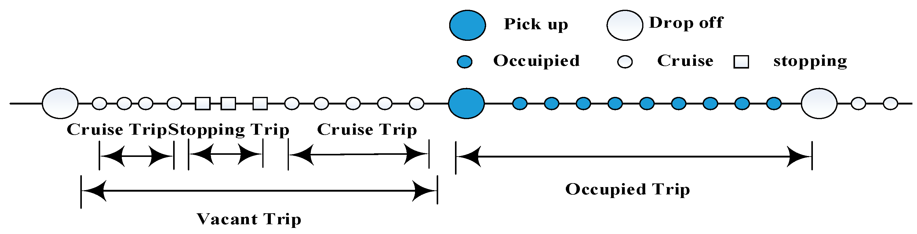
Figure 2.
Distance calculation methods: Euclidian distance and the spherical law of cosines.

Figure 3.
Cluster result of driving profitability.
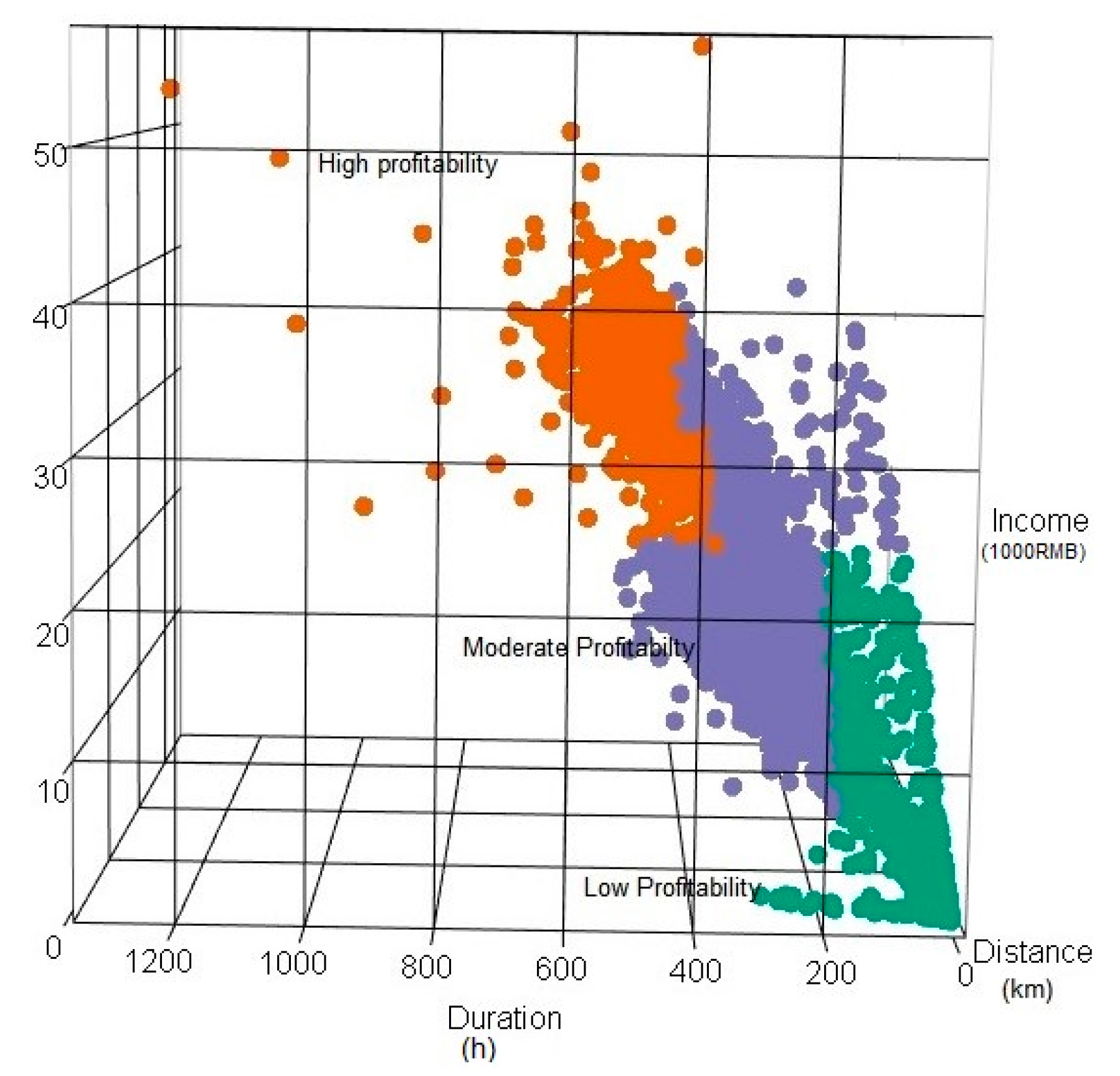
Figure 4.
Occupancy ratio of high, moderate and low profitability drivers.

Figure 5.
Frequency distribution of the cruising trip time of low (a), moderate (b) and high (c) profitability drivers.
Figure 5.
Frequency distribution of the cruising trip time of low (a), moderate (b) and high (c) profitability drivers.

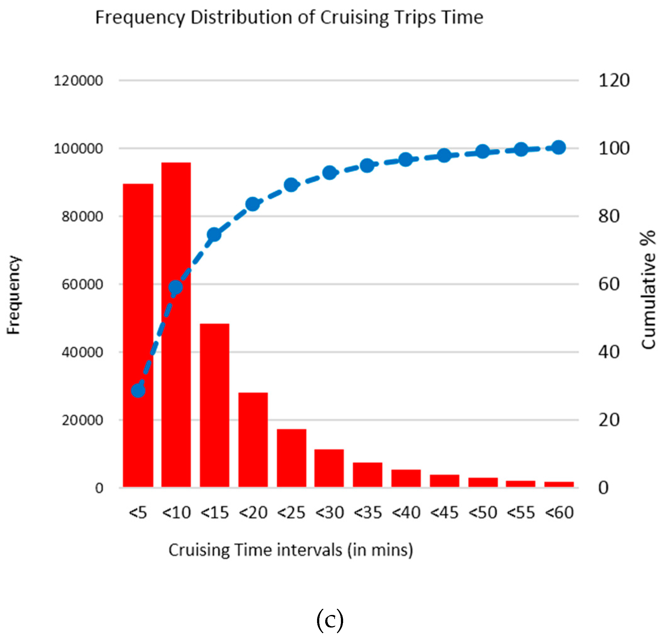
Figure 6.
Spatial distribution of cruising trips of high (a), moderate (b) and low (c) profitability drivers.
Figure 6.
Spatial distribution of cruising trips of high (a), moderate (b) and low (c) profitability drivers.

Figure 7.
Hourly average distribution of stopping spots.
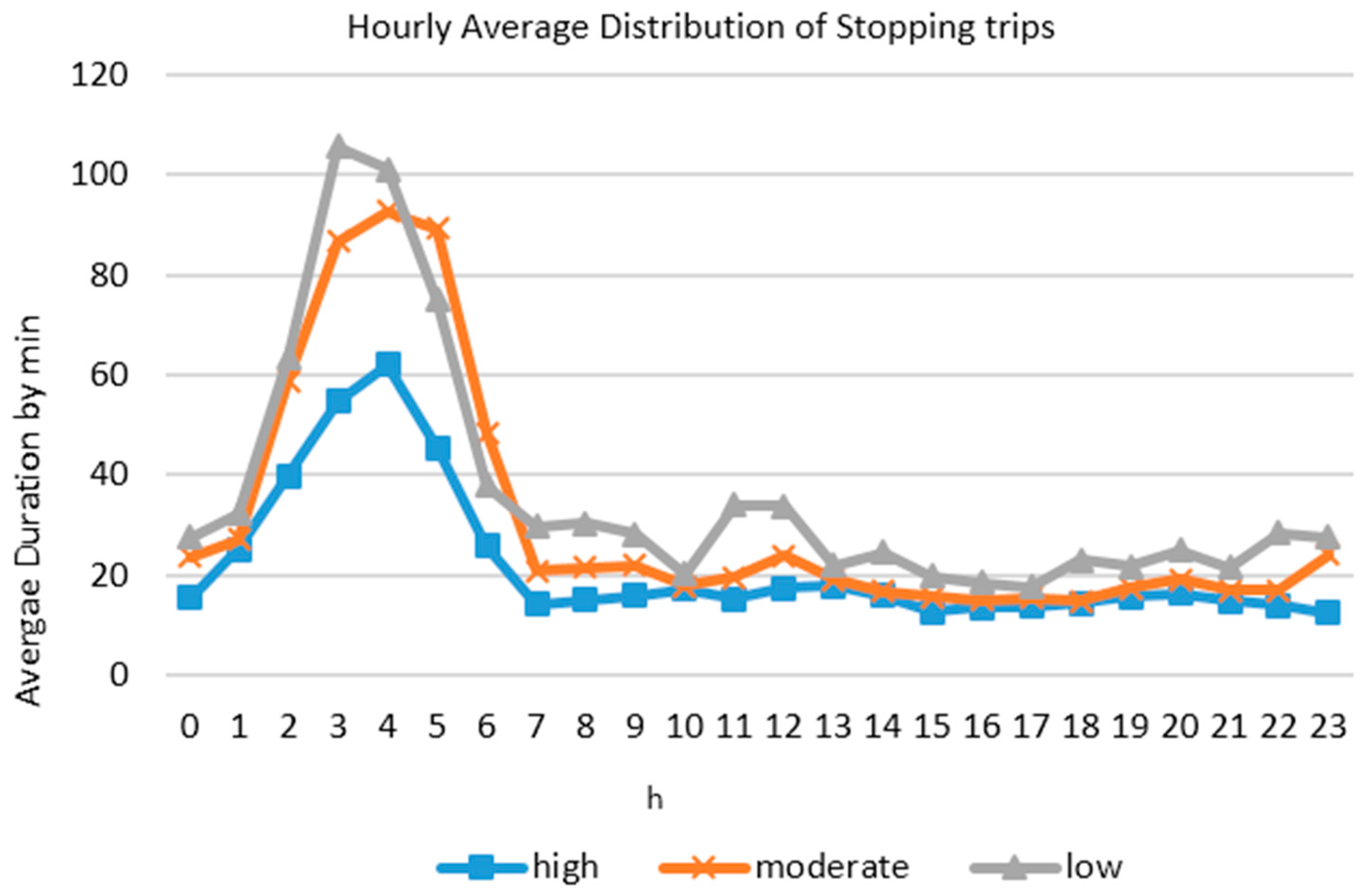
Figure 8.
Spatial and temporal patterns of stopping spots of high (a), moderate (b) and low (c) profitability drivers for longer durations.
Figure 8.
Spatial and temporal patterns of stopping spots of high (a), moderate (b) and low (c) profitability drivers for longer durations.

Figure 9.
Stopping spots of the off-peak duration of high (a), moderate (b) and low (c) profitability drivers.
Figure 9.
Stopping spots of the off-peak duration of high (a), moderate (b) and low (c) profitability drivers.

Figure 10.
Average stopping duration of off-peak of high, moderate and low profitability drivers.


Table 1.
Description of the fields of the taxi GPS data.
| Field | Value | Description |
|---|---|---|
| Driver ID | 23300123 | 8-digit number |
| Timestamp | 20131001000830 | 14-digit number 1 October 2013 00:08:30 |
| Longitude | 30.587833 | Accurate to 6 decimal places, in degrees |
| Latitude | 114.343916 | Accurate to 6 decimal places, in degrees |
| Velocity | 63.6 | in km/h |
| Car Status | 0, 1, 2, 3 | 1, not occupied; 2, temporarily stopped; 3, occupied; 0, GPS device signal is invalid |
Table 2.
Description of each taxi state.
| Taxi State | Description | |
|---|---|---|
| Occupied (O) | A taxi is loaded and occupied by a passenger | |
| Vacant (V) | Cruise (C) | A taxi is traveling without a passenger |
| Stopping (S) | A taxi is static without a passenger | |
Table 3.
Taxi fare system of Wuhan City in 2013.
| Item | Price | |
|---|---|---|
| P0 | Within 2 km | 6 Yuan |
| P2 | Within 2–7 km | 1.5 Yuan/km |
| P7 | Exceed 7 km | 2.1 Yuan/km |
| FS | Extra Oil Surcharge | 2 Yuan/trip |
Table 4.
Examples of occupied trips’ information.
| Taxi ID_Tripid | Trip Duration | Trip Spatial Data | Fare | ||||
| Pick-up Time | Drop-off Time | Duration (min) | Pick-up (log, lat) | Drop-off (log, lat) | Distance (km) | ||
| 2618113_1 | 00:51:34 | 01:00:53 | 9 | (30.550, 114.316) | (30.593, 114.258) | 10 | 22 |
| 2871041_3 | 06:27:59 | 06:54:13 | 27 | (30.968, 114.229) | (30.557, 114,210) | 20 | 42.8 |
| 1020463_8 | 13:16:45 | 13:55:49 | 39 | (30.772, 114.206) | (30.593, 114.339) | 36 | 76.4 |
log, lat represent the longitude and latitude of a point in a map, respectively.
Table 5.
Characteristics of driving profitability groups.
| Profitability Groups | Number of Drivers | % | Mean of Driving Profitability Features | ||
|---|---|---|---|---|---|
| Distance (km) | Duration (hours) | Income (1000 RMB) | |||
| Low group | 844 | 18 | 2.05 | 76.5 | 8.69 |
| Moderate group | 2116 | 45.1 | 6.6 | 288.2 | 18.8 |
| High group | 1722 | 36.7 | 9 | 450.5 | 30.3 |
Table 6.
Total number of the three types trips of the three profitability levels of the taxi drivers.
Table 6.
Total number of the three types trips of the three profitability levels of the taxi drivers.
| Profitability Level | Occupied | Cruising | Stopping |
|---|---|---|---|
| High | 298,779 | 314,086 | 32,668 |
| Low | 230,678 | 300,621 | 28,120 |
| Moderate | 287,801 | 358,364 | 32,225 |
© 2017 by the authors. Licensee MDPI, Basel, Switzerland. This article is an open access article distributed under the terms and conditions of the Creative Commons Attribution (CC BY) license (http://creativecommons.org/licenses/by/4.0/).
Share and Cite
MDPI and ACS Style
Naji, H.A.H.; Wu, C.; Zhang, H. Understanding the Impact of Human Mobility Patterns on Taxi Drivers’ Profitability Using Clustering Techniques: A Case Study in Wuhan, China. Information 2017, 8, 67. https://doi.org/10.3390/info8020067
AMA Style
Naji HAH, Wu C, Zhang H. Understanding the Impact of Human Mobility Patterns on Taxi Drivers’ Profitability Using Clustering Techniques: A Case Study in Wuhan, China. Information. 2017; 8(2):67. https://doi.org/10.3390/info8020067
Chicago/Turabian StyleNaji, Hasan A. H., Chaozhong Wu, and Hui Zhang. 2017. "Understanding the Impact of Human Mobility Patterns on Taxi Drivers’ Profitability Using Clustering Techniques: A Case Study in Wuhan, China" Information 8, no. 2: 67. https://doi.org/10.3390/info8020067
Note that from the first issue of 2016, this journal uses article numbers instead of page numbers. See further details here.