
Assembling Deep Neural Networks for Medical Compound Figure Detection


1
School of Computer Science and Technology, Dalian University of Technology, Dalian 116024, China
2
School of Computer Science & Engineering, Dalian Minzu University, Dalian 116600, China
3
School of Software Engineering, Dalian University of Foreign Language, Dalian 116044, China
*
Author to whom correspondence should be addressed.
Information 2017, 8(2), 48; https://doi.org/10.3390/info8020048
Submission received: 17 March 2017
/
Revised: 18 April 2017
/
Accepted: 19 April 2017
/
Published: 21 April 2017
Abstract
:Compound figure detection on figures and associated captions is the first step to making medical figures from biomedical literature available for further analysis. The performance of traditional methods is limited to the choice of hand-engineering features and prior domain knowledge. We train multiple convolutional neural networks (CNNs), long short-term memory (LSTM) networks, and gated recurrent unit (GRU) networks on top of pre-trained word vectors to learn textual features from captions and employ deep CNNs to learn visual features from figures. We then identify compound figures by combining textual and visual prediction. Our proposed architecture obtains remarkable performance in three run types—textual, visual and mixed—and achieves better performance in ImageCLEF2015 and ImageCLEF2016.
1. Introduction
With the development of the Internet, the amount of biomedical literature in electronic format has increased considerably [1]. The large-scale figures in the articles have become valuable to medical education, medical research and clinical diagnosis [2]. It is difficult to manage such a substantial repository of information appropriately. This prompts the development of methods for the automatic classification of medical figures in order to improve the ability to retrieve relevant images.
Many images in the biomedical literature (over 40% [3]) are compound figures (see Figure 1). Medical image retrieval systems, such as OPENi [4], have been cross-media-based, relying on the captions associated with the images as the input to the retrieval system. Users of OPENi can filter the compound figures by selecting “Image Type” as “Exclude Multipanel” to reduce the range of search. Compound figure identification is the first step to making compound images from the literature available for further analysis, such as multi-label classification, compound figure separation, subfigure modality classification, and caption generating. To facilitate research and development in this field, the Image Cross-Language Evaluation Forum (ImageCLEF) has run the medical task since 2004. The subtask of compound figure detection was first introduced in ImageCLEF2015 [5] and continued in ImageCLEF2016 [6]. The goal of this subtask is to identify whether a figure is a compound figure or not. The subtask makes training data and test data containing compound figures and non-compound figures and their related captions from the biomedical literature available.
This recognition task involves three run types—textual, visual and mixed. Characteristic Delimiters [9] and Bag-of-Words (BoW) are used to extract textual features. With respect to visual methods, most researchers focus on low level features such as Border Profile [9,10,11], Bag-of-Keypoints (BoK) [12], Bag-of-Colors (BoC) [13], and SURFContext [14]. The best results are obtained by a combination of cross-media predictions [5,6]. Although achieving a good performance, the hand-design features mentioned above are dependent on the choice of features and demand a clear awareness of the prior domain knowledge. Hence, it is hard to capture a substantial number of possible input variations very well.
Recently, deep neural networks attain remarkable achievements in not only computer vision (CV) but also natural language processing (NLP). Convolutional neural networks (CNNs) [15] have led to a series of breakthroughs for image classification [16,17,18]. Within NLP, most of the work with deep learning models, such as Convolutional neural network (CNN) for sentence classification [19,20], long short-term memory (LSTM) [21], networks for sentiment classification [22,23], and gated recurrent unit (GRU) networks [24] for sentiment classification [23], involve learning word vector representations [25] and performing compositions over the learned word vectors for classification.
Our group of DUTIR (Information Retrieval Laboratory of Dalian University of Technology) took part in the subtask of compound figure detection in ImageCLEF2016 and achieved good performance [6]. However, our textual runs based on CNN or (Recurrent Neural Network) RNN had not obtained state-of-the-art accuracy on textual run type. In this work, we employ several different neural networks and realize, without much surprise, that model combination performs better than any individual technique. We train several networks of CNN, LSTM, and GRU to learn features from captions over pre-trained word vectors to make textual predictions. As for visual prediction, we still feed original figures to make a visual model of multiple deep CNNs. Finally, we combine two types of results to identify compound figures.
We test our mixed models on datasets of both ImageCLEF2015 and ImageCLEF2016 and obtain better accuracies of 88.07% and 96.24%, compared to 85.39% in ImageCLEF2015 [5] and 92.7% in ImageCLEF2016 [6]. We also evaluate rule-based neural networks on text or images and achieve good performance of both textual and visual prediction, respectively. However, our rule-based mixed model is unable to improve performance. These results show that our cross-media framework can effectively capture the “rule” information from a compound figure and its caption.
2. Methods
This section describes the architecture of assembling neural networks (NNs) (see Figure 2). Our system contains one cross-media mixed model without rules (Mixed Model) and two single-media models based on rules (Model of Delimiter and Model of Border). A Model of Delimiter is one textual rule model based on Delimiter Features and three deep learning methods of textual convolutional neural networks (TCNNs), textual long short-term memory networks (TLSTMs) and textual gated recurrent unit networks (TGRUs). A Model of Border is composed of Border Features and visual convolutional neural networks (VCNNs).
2.1. Textual Methods
Before pre-training the word vectors, we extract all captions from both training set and test set. Using Stanford CoreNLP tools [26], we tokenize the texts but retain the delimiters such as “a)”, “b)”, “c)”, or “(a)”, “(b)”, “(c)”.
In ImageCLEF2015 or ImageCLEF2016, we obtain one word vector vocabularies trained on 6.8 million words collected from all captions, using the word2vec tool created by Mikolov et al. [25], which provides an efficient implementation of the continuous bag-of-words and skip-gram architectures for computing vector representations of words. The vectors have a dimensionality of 300. Words not presented in the set of pre-trained words are initialized randomly.
Each sentence is wrapped to a window of 300 words to reduce the number of parameters. Maximum sentence length is 300, longer sentences are truncated and shorter sentences are padded with zeros at the end.
Using binary cross entropy to define the loss function, we separately trained three textual neural network models of TCNNs, TLSTMs, and TGRUs (see Figure 2) on top of the pre-trained word vectors. We set word2vec vectors as our embedding layer’s weights and use Glorot uniform [27] initializer to initial training weights of our neural networks. After gathering the outputs of three textual NNs models, we feed them to the next step of cross-media combination (discussed in a later subsection) or a textual combination based on Delimiter Features.
2.1.1. Textual Convolutional Neural Networks
The model of TCNNs, shown in Figure 2, is similar to the CNN architecture [19,28] with an embedding layer with a dropout of 0.25, a convolutional layer with a kernel size of 3 and 250 feature maps, a max-over-time pooling layer with a max-pool size of 2, a vanilla layer with 250 neurons, a dropout of 0.25, and a ReLU (Rectified Linear Unit) activation function, and a full-connected layer with 2 neurons. The softmax function is implemented at the final layer to output the prediction probabilities of two classes. After training multiple (e.g., 5) networks through the RMSProp optimizer [29] over shuffled mini-batches of 32, we take averaging prediction results as the output of the model.
2.1.2. Textual Long Short-Term Memory Network
The model of TLSTMs, shown in Figure 2, applies dropout within the LSTM layer similar to [23,30]. The architecture of this model contains an embedding layer with a dropout of 0.5, an LSTM layer with a dropout of 0.5, a full-connected layer with 2 neurons, and a softmax layer. We train multiple (e.g., 5) networks through Adam (Adaptive Moment Estimation) [31] over shuffled mini-batches of 32 and make the prediction by averaging all results.
2.1.3. Textual Gated Recurrent Unit Network
The model of TGRUs, shown in Figure 2, also applies a dropout within the GRU layer similar to [23,24]. The model consists of an embedding layer with a dropout of 0.5, a GRU layer with a dropout of 0.5, a full-connected layer with 2 neurons, and a softmax layer. After training multiple networks through Adam [31] over shuffled mini-batches of 32, we also combine them by averaging all results.
2.1.4. Textual Rule Model of Delimiter
When captions of compound figures are written, it is most likely that existing subfigures are addressed using some delimiters. Therefore, we extract three-dimensional Characteristic Delimiter features [9] from the caption of the input figure. We select delimiters with the highest occurrence in the captions referred as “Characteristic Delimiters.” By analyzing these captions from the training set, we finally select three delimiter pairs of “a, b”, “a), b)” and “(a), (b)” to compute a feature vector by detecting whether one pair of them exists.
Then we feed these features to a Logistic Regression (LR) classifier to output prediction probabilities of compound figures. After that, we combine the output with other NNs models by assigning the deciding vote of positive prediction to the LR classifier. Specifically, for each sample, we take the output of the LR classifier as the prediction when it makes a positive prediction, or use the output of the NN models. The new outputs of these rule-based models are taken as the textual predictions of input samples.
2.2. Visual Methods
2.2.1. Visual Convolutional Neural Networks
Before inputting the figures into VCNNs, shown in Figure 2, we resize them to a square of N × N pixels (where N = 32, 64, 128, etc.) and prepare a Python version of the dataset similar to the CIFAR-10 Python dataset.
The model of VCNNs is a deep CNN similar to [28,32,33]. The first two convolutional layers contain 32 kernels of size 3 × 3, and the second two convolutional layers have 32 kernels of size 3 × 3. The second and fourth convolutional layers are interleaved with pooling layers of dimension 2 × 2 with a dropout of 0.25. Then, a full-connected layer with 512 neurons and a dropout of 0.5 is followed by a full-connected layer with 2 neurons. ReLU activation function is applied to all four convolutional layers and the first full-connected layer. The softmax function is implemented at the final layer to output the prediction probabilities of two classes. We use Glorot uniform to initial training weights and train the model using stochastic gradient descent (SGD) over shuffled mini-batches of 32.
2.2.2. Visual Rule Model of Border
A highly distinguishing feature characterizing a compound figure is the existence of a separating border. We extract four-dimensional Border Features similar to [9] from input figures to describe the presence of these horizontal or vertical and black or white borders.
Firstly, we resize the figure to a square of 256 × 256 pixels and detect the presence of borders. We choose a strict detecting range of [80, 170] from two directions to attain greater precision. Then we feed these features to the Logistic Regression classifier with the same parameters as the textual rules of the Model of Delimiter and combine the results with the NN model in a way similar to the Model of Delimiter. The new outputs of this model are taken as the visual prediction of input samples.
2.3. Mixed Method
The predictions are combined mentioned above using the same average strategy:
where is the prediction class label, the function of returns the mean of the input predicted probabilities of models, and the function of () refers to the input , at which the output of average is maximum.
Our Mixed Model: after combining three textual models with the visual model separately, we fuse the three cross-media combinations without rules by using average strategy again to make a final mixed prediction of the current sample.
3. Experiments
In this section, we describe baseline models, which get the highest accuracies of Compound Figure Detection task in ImageCLEF 2015 and ImageCLEF 2016, in comparison with our proposed models. Then, we present the experimental results of our approaches as well as the baseline.
3.1. Dataset
For our experiments, we utilize the ImageCLEF 2015 and ImageCLEF2016 Compound Figure Detection dataset [5,6] using a subset of PubMed Central. This task makes training data and test data available containing compound and non-compound figures from the biomedical literatures. ImageCLEF provides figures and associated captions, each pair of which is labeled as compound figure (COMP) or non-compound figure (NOCOMP). In ImageCLEF 2015 [5], the training set contains 10,433 figures and the test set 10,434 figures. Each of these two sets contains 6144 compound figures. In ImageCLEF 2016 [6], they expand their training set to 20,997 figures and reduce the size of the test set to 3456. These two sets contain 12,348 and 1806 compound figures, respectively.
In accordance with the evaluation criterion of the benchmark, we evaluate our approach based on two-class (COMP and NOCOMP) classification accuracy for all experiments unless otherwise stated. After training the networks with 10-fold cross validation (10FCV) on the training set, we test our trained models on the test set. Many codes have been modified from our previous work [28,32,33] and are implemented with the neural network library of Keras, running on top of TensorFlow. All default parameters are used, except for those parameters mentioned in Section 2. Our networks are trained on one NVIDIA Tesla K20c GPU in a 64 bit Dell computer with two 2.40 GHz CPUs, 64 G main memories in Dalian, China, and Ubuntu 12.04.
3.2. Baselines
This section describes the baseline methods, and their results in both ImageCLEF2015 and ImageCLEF2016.
3.2.1. ImageCLEF2015
Pelka et al. [9] obtained the best textual result with an accuracy of 78.34% in ImageCLEF2015 labeled as Baseline_Text (see Table 1). With respect to textual features, they used Bag-of-Words (BoW) approach using the provided figure caption. They also detected the presence of some delimiters characterizing compound figure, which were manually selected by analyzing the associated captions from the training set. After concatenating BoW features and Characteristic Delimiter features, they fed them to a random forest (RF) classifier.
Wang et al. [10] obtained the best visual result with an accuracy of 82.82% in ImageCLEF2015 labeled as Baseline_Figure (see Table 2). They fused two different schemes to identify the compound figure. The connected component analysis-based scheme mainly addressed the issue of the presence of the connected text in the compound figures using special ratio criterions. The peak region detection-based scheme leveraged pixel intensity to find borders.
Pelka et al. [8] achieved the best result using a multi-modal approach, with an accuracy of 85.39% in ImageCLEF2015 labeled as Baseline_Mixed (see Table 3). They extracted Bag-of-Keypoints (BoK) features and Borders Features from figures. After reducing the feature dimensions using principal component analysis, they concatenated the visual features and the textual features mentioned above and fed them to the random forest (RF) classifier.
3.2.2. ImageCLEF2016
In ImageCLEF2016, very good results were obtained for the compound figure detection task, reaching up to 92.7% for our team (DUTIR) labeled as Baseline_Mixed (see Table 3). Our team also obtained the best visual result with an accuracy of 92.01%, labeled as Baseline_Figure (see Table 2), by combining five deep convolutional neural networks. MLKD obtained the best textual result of 88.13% labeled as Baseline_Text (see Table 1).
3.3. Experimental Results and Discussion
3.3.1. Textual Results
We use the following protocol for all textual experiments: maximum input sentence length of 300, a mini-batch size of 32, and an epoch number of 6. We choose these values via a grid search on the ImageCLEF2015 dataset.
From Table 1, we can see that the performance of any type of neural network (NN) models (TCNN1, TLSTM1, and TGRU1) have been better than the baseline of textual models both in ImageCLEF2015 and in ImageCLEF2016. Inspired by the work of [28,32,33], we train five networks with the same structure for each of three textual models and combine them separately (TCNN5, TLSTM5, and TGRU5, see Table 1) to improve performance further. For example, among three types of textual models, the textual convolutional neural network (TCNN5) obtains the performance of 82.30% in ImageCLEF2015 and 89.81% in ImageCLEF2016, which are both higher than textual baseline of 78.34% and 88.13% (Baseline_Text).
After feeding the characteristic delimiters features to an LR classifier with the inverse of regularization strength of , implemented on Scikit-Learn tools, we obtain a lower accuracy of 81.42% and 83.91% (see Table 1). However, a further observation shows that the Model of Delimiter has higher precisions than those of other NN models (see Table 4) in both 2015 and 2016. They also surpass the accuracy of the NN models for the same subset samples, which are identified as positive by the LR classifier trained on Delimiter Features (see Table 4). This advantage of Delimiter results in that all NN models improve their performance when combined with the textual rule (see Table 1). For example, the accuracy of the model of five rule-based textual Gated Recurrent Unit networks (Rule_TGRU5) gains a more than 0.80% point increase (from 82.40% to 83.24% in 2015 and from 88.72% to 89.53% in 2016).
Finally, we combine all three rule-based textual NN models to construct a Model of Delimiter to identify compound figures and obtain state-of-the-art textual accuracy of 83.24% in ImageCLEF2015 and 90.25% in ImageCLEF2016.
3.3.2. Visual Results
We use the following protocol for the experiment of visual neural networks model: a -batch size of 32, an epoch number of 30, and an image size of 64.
Similar to our textual models, we also train five deep CNNs with the same structure on figures, and combine their results to identify compound figures. This combination obtains an over 3% point increase (from 80.83% to 84.24% in 2015 and from 89.99% to 92.33% in 2016) (see Table 2).
We find a similar advantage when observing the performance of the visual models. For the same subset samples recognized as positive by the LR classifier trained on Border Features, it has a higher accuracy than those of NNs model (92.86% versus 90.76% in 2015 and 95.58% versus 95.32% in 2016) (see Table 5). These results can explain well why rule-based neural networks (Model of Border) attain a better visual accuracy of 86.28% in 2015 and 93.66% in 2016 (see Table 2).
3.3.3. Mixed Results
We combine three types of textual neural networks with visual networks separately and compare their prediction probabilities. The results show that assembling all combinations achieves more stable performance than any single one (see Table 3). Our system obtains better accuracies of 88.07% in 2015 and 96.24% in 2016.
We also test to combine textual and visual neural networks based on rules to identify compound figures. From Table 3, we find that introducing rule information into our cross-media combination cannot effectively improve performance of prediction. When combining all three mixed models based on rule, it even harms the performance (from 88.07% to 87.52% in 2015 and from 96.24% to 96.18% in 2016). In a similar way, we create a subset whose samples are identified as positive by Logistic Regression trained on Delimiter or Border Features and compare the performance of rule models with three cross-media combinations without rules (see Table 6 and Table 7).
We further explore the results to find the reasons that the performance drops after we include rules in the system. On one hand, from Table 4 and Table 5, we can see the rule methods have very badly recalls (take visual methods’ as an example: 56.94% in 2015 and 59.91% in 2016), although their precisions are better than neural networks methods based on single media. On the other hand, our cross-media methods have better precision than the LR classifiers based on rules (see Table 6 and Table 7). These results show that our cross-media combinations can capture well the compound figure information from both figures and captions.
3.3.4. Running Time
The training times of our networks are listed in Table 8. For comparative purposes, we present the running time on training or testing one sample excluding data preprocessing times. For deep learning models, we record the training time in one epoch. From Table 8, we find that the traditional feature-engineering method is much faster than neural networks method. In our experiments, CNNs tend to be much faster than RNNs.
4. Conclusions
We have presented a system for medical compound figure identification that is composed of two independent parts, the visual and the textual, which are combined by averaging the prediction probabilities. Our system achieves promising performance in the ImageCLEF2015 and ImageCLEF2016 compound figure detection tasks of the visual, the textual, and the mixed. We hope to include new techniques into our system and focus on improving the state of the art for this task.
Acknowledgments
This research was supported by the National Natural Science Foundation of China (No. 61272373, No. 61202254, and No. 71303031) and the Fundamental Research Funds for the Central Universities (No. DC13010313 and No. DC201502030202). The authors also gratefully acknowledge the helpful comments and suggestions of the reviewers, which improve the presentation.
Author Contributions
Yuhai Yu designed and wrote paper; Hongfei Lin supervised the work; Xiaocong Wei and Jiana Meng conceived and designed the experiments; Yuhai Yu and Zhehuan Zhao performed the experiments; Yuhai Yu analyzed the data. All authors have read and approved the final manuscript.
Conflicts of Interest
The authors declare no conflict of interest.
References
- Lu, Z. PubMed and beyond: A survey of web tools for searching biomedical literature. Database 2011, 2011. [Google Scholar] [CrossRef] [PubMed]
- Müller, H.; Despont-Gros, C.; Hersh, W.; Jensen, J.; Lovis, C.; Geissbuhler, A. Health care professionals’ image use and search behavior. In Proceedings of the Medical Informatics Europe, Maastricht, The Netherlands, 27–30 August 2006. [Google Scholar]
- De Herrera, A.G.S.; Kalpathy-Cramer, J.; Fushman, D.D.; Antani, S.; Müller, H. Overview of the ImageCLEF 2013 medical tasks. In Proceedings of the Working Notes of CLEF, Valencia, Spain, 23–26 September 2013. [Google Scholar]
- Demner-Fushman, D.; Antani, S.; Simpson, M.; Thoma, G.R. Design and development of a multimodal biomedical information retrieval system. J. Comput. Sci. Eng. 2012, 6, 168–177. [Google Scholar] [CrossRef]
- De Herrera, A.G.S.; Müller, H.; Bromuri, S. Overview of the ImageCLEF 2015 medical classification task. In Proceedings of the Working Notes of CLEF, Toulouse, France, 8–11 September 2015. [Google Scholar]
- De Herrera, A.G.S.; Schaer, R.; Bromuri, S.; Müller, H. Overview of the ImageCLEF 2016 medical task. In Proceedings of the Working Notes of CLEF, Évora, Portugal, 5–8 September 2016. [Google Scholar]
- Plataki, M.; Tzortzaki, E.; Lambiri, I.; Giannikaki, E.; Ernst, A.; Siafakas, N.M. Severe airway stenosis associated with Crohn’s disease: Case report. BMC Pulm Med. 2006, 6, 7. [Google Scholar] [CrossRef] [PubMed]
- Theegarten, D.; Sachse, K.; Mentrup, B.; Fey, K.; Hotzel, H.; Anhenn, O. Chlamydophila spp. infection in horses with recurrent airway obstruction: Similarities to human chronic obstructive disease. BMC Respir. Res. 2008, 9, 14. [Google Scholar] [CrossRef] [PubMed]
- Pelka, O.; Friedrich, C.M. FHDO biomedical computer science group at medical classification task of ImageCLEF 2015. In Proceedings of the Working Notes of CLEF, Toulouse, France, 8–11 September 2015. [Google Scholar]
- Wang, X.; Jiang, X.; Kolagunda, A.; Shatkay, H.; Kambhamettu, C. CIS UDEL Working Notes on ImageCLEF 2015: Compound figure detection task. In Proceedings of the Working Notes of CLEF 2015, Toulouse, France, 8–11 September 2015. [Google Scholar]
- De Herrera, A.G.S.; Markonis, D.; Schaer, R.; Eggel, I.; Müller, H. The medGIFT Group in ImageCLEFmed 2013. In Proceedings of the Working Notes of CLEF, Valencia, Spain, 23–26 September 2013. [Google Scholar]
- Csurka, G.; Dance, C.; Fan, L.; Willamowski, J.; Bray, C. Visual Categorization with Bags of Keypoints. In Proceedings of the Workshop on Statistical Learning in Computer Vision, European Conference on Computer Vision, Prague, Czech Republic, 11–14 May 2004. [Google Scholar]
- De Herrera, A.G.S.; Markonis, D.; Müller, H. Bag-of-Colors for Biomedical Document Image Classification. Proceedings of Medical Content-Based Retrieval for Clinical Decision Support (MCBR-CDS), Nice, France, 1 October 2012. [Google Scholar]
- Zhou, X. Grid-Based Medical Image Retrieval Using Local Features. Ph.D. Thesis, University of Geneva, Geneva, Switzerland, November 2011. [Google Scholar]
- LeCun, Y.; Bottou, L.; Bengio, Y.; Haffner, P. Gradient-based learning applied to document recognition. Proc. IEEE 1998, 86, 2278–2324. [Google Scholar] [CrossRef]
- Krizhevsky, A.; Sutskever, I.; Hinton, G.E. Imagenet classification with deep convolutional neural networks. In Proceedings of the Advances in Neural Information Processing Systems, Lake Tahoe, NV, USA, 3–6 December 2012. [Google Scholar]
- Szegedy, C.; Liu, W.; Jia, Y.; Sermanet, P.; Reed, S.; Anguelov, D.; Erhan, D.; Vanhoucke, V.; Rabinovich, A. Going deeper with convolutions. In Proceedings of the IEEE Conference on Computer Vision and Pattern Recognition, Boston, MA, USA, 7–12 June 2015. [Google Scholar]
- He, K.; Zhang, X.; Ren, S.; Sun, J. Deep Residual Learning for Image Recognition. arXiv 2015. [Google Scholar]
- Kim, Y. Convolutional neural networks for sentence classification. arXiv 2014. [Google Scholar]
- Collobert, R.; Weston, J.; Bottou, L.; Karlen, M.; Kavukcuoglu, K.; Kuksa, P. Natural language processing (almost) from scratch. J. Mach. Learn. Res. 2011, 12, 2493–2537. [Google Scholar]
- Hochreiter, S.; Schmidhuber, J. Long Short-Term Memory. Neural Comput. 1997, 9, 1735–1780. [Google Scholar] [CrossRef] [PubMed]
- Tai, K.S.; Socher, R.; Manning, C.D. Improved semantic representations from tree-structured long short-term memory networks. arXiv 2015. [Google Scholar]
- Gal, Y.A. Theoretically Grounded Application of Dropout in Recurrent Neural Networks. arXiv 2015. [Google Scholar]
- Cho, K.; Van Merriënboer, B.; Bahdanau, D.; Bengio, Y. On the Properties of Neural Machine Translation: Encoder–Decoder Approaches. arXiv 2014. [Google Scholar]
- Mikolov, T.; Dean, J. Distributed representations of words and phrases and their compositionality. In Proceedings of the Advances in Neural Information Processing Systems, Lake Tahoe, NV, USA, 5–10 December 2013. [Google Scholar]
- Manning, C.D.; Surdeanu, M.; Bauer, J.; Finkel, J.R.; Bethard, S.; McClosky, D. The stanford corenlp natural language processing toolkit. In Proceedings of the 52nd Annual Meeting of the Association for Computational Linguistics: System Demonstrations, Baltimore, MD, USA, 22–27 June 2014. [Google Scholar]
- Glorot, X.; Bengio, Y. Understanding the difficulty of training deep feedforward neural networks. In Proceedings of the 13th International Conference on Artificial Intelligence and Statistics (AISTATS), Sardinia, Italy, 13–15 May 2010. [Google Scholar]
- Yu, Y.; Lin, H.; Meng, J.; Zhao, Z. Visual and Textual Sentiment Analysis of a Microblog Using Deep Convolutional Neural Networks. Algorithms 2016, 9. [Google Scholar] [CrossRef]
- Tieleman, T.; Hinton, G. Divide the gradient by a running average of its recent magnitude. COURSERA: Neural networks for machine learning, Technical Report. Available online: https://zh.coursera.org/learn/neural-networks/lecture/YQHki/rmsprop-divide-the-gradient-by-a-running-average-of-its-recent-magnitude (accessed on 21 April 2017).
- Graves, A. Generating sequences with recurrent neural networks. arXiv 2013. [Google Scholar]
- Kingma, D.; Ba, J. Adam: A method for stochastic optimization. arXiv 2014. [Google Scholar]
- Yu, Y.; Lin, H.; Meng, J.; Zhao, Z.; Li, Y.; Zuo, L. Modality classification for medical images using multiple deep convolutional neural networks. JCIS 2015, 11, 5403–5413. [Google Scholar]
- Wan, L.; Zeiler, M.; Zhang, S.; Cun, Y.L.; Fergus, R. Regularization of neural networks using dropconnect. In Proceedings of the 30th International Conference on Machine Learning (ICML-13), Atlanta, GA, USA, 16–21 June 2013. [Google Scholar]
Figure 1.
Examples of compound figure and non-compound figure. (a) Compound figure adapted from [7]: computed tomography (CT). (b) Non-compound figure adapted from [8]: immunohistochemistry of equine lung tissue in Recurrent Airway Obstruction (RAO).
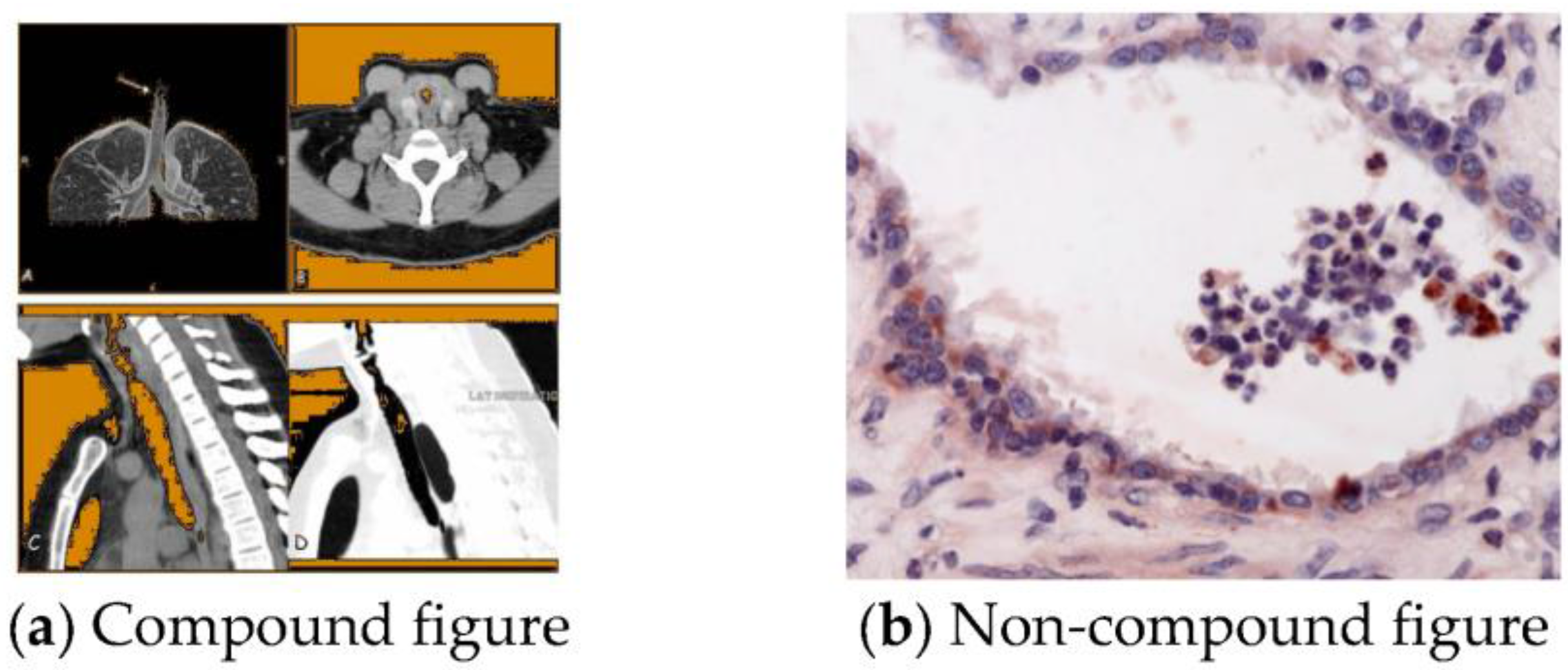
Figure 2.
Architecture of assembling deep neural networks for compound figure detection.


Table 1.
Accuracy of textual methods.
| Models 2 | ImageCLEF2015 (%) | ImageCLEF2016 (%) | ||
|---|---|---|---|---|
| 10FCV | Evaluation | 10FCV | Evaluation | |
| Baseline_Text | - | 78.34 | - | 88.13 |
| TCNN1 | 86.10 ± 0.12 | 82.24 ± 0.16 1 | 85.18 ± 0.14 | 89.38 ± 0.25 |
| TCNN5 | 86.37 | 82.30 | 85.75 | 89.81 |
| TLSTM1 | 86.50 ± 0.57 | 81.09 ± 0.54 | 85.15 ± 0.19 | 87.69 ± 0.25 |
| TLSTM5 | 87.16 | 81.67 | 85.84 | 88.69 |
| TGRU1 | 87.18 ± 0.07 | 82.01 ± 0.20 | 85.10 ± 0.71 | 88.28 ± 0.72 |
| TGRU5 | 87.23 | 82.40 | 85.91 | 88.72 |
| LR + Delimiter Features | 82.36 | 81.42 | 81.82 | 83.91 |
| Rule_TCNN5 | 87.38 | 82.61 | 86.45 | 90.05 |
| Rule_TLSTM5 | 87.50 | 81.90 | 86.14 | 89.53 |
| Rule_TGRU5 | 87.23 | 83.24 | 86.38 | 89.53 |
| TCNN5 + TLSTM5 + TLSTM5 | 87.89 | 82.95 | 86.49 | 89.90 |
| Model of Delimiter | 88.02 | 83.24 | 86.62 | 90.25 |
1 “82.24 ± 0.16” means the average accuracy of 82.24 with the standard deviation of 0.16. 2 “Models” contains three textual NNs (“TCNN”, “TLSTM”, and “TGRU”) models, three rule-based textual NNs models (“Rule_TCNN”, “Rule_TLSTM”, and “Rule_TLSTM”), two kinds of combination, and a rule-based Model of Delimiter, in addition to baseline model of “Baseline_Text”. The suffix “1” or “5” indicates the number of networks trained.
Table 2.
Accuracy of visual methods.
| Models 1 | ImageCLEF2015 (%) | ImageCLEF2016 (%) | ||
|---|---|---|---|---|
| 10FCV | Test | 10FCV | Test | |
| Baseline_Figure | - | 82.82 | - | 92.01 |
| VCNN1 | 85.40 ± 0.12 | 80.83 ± 0.45 | 86.41 ± 0.43 | 89.99 ± 0.44 |
| VCNN5 | 88.27 | 84.24 | 89.50 | 92.33 |
| LR + Border Features | 70.36 | 72.98 | 71.76 | 77.60 |
| Model of Border | 89.05 | 86.28 | 90.22 | 93.66 |
1 “Models” contain visual CNN (“VCNN1” and “VCNN5”) models and one visual rule model based on Border Features and CNNs (“Model of Border”), in addition to baseline model of “Baseline_Text”. The suffix “1” or “5” indicates the number of networks trained.
Table 3.
Accuracy of mixed methods.
| Models | ImageCLEF2015 (%) | ImageCLEF2016 (%) | ||
|---|---|---|---|---|
| 10FCV | Test | 10FCV | Test | |
| Baseline_Mixed | - | 85.39 | - | 92.70 |
| TCNN5 + VCNN5 | 91.30 | 87.93 | 89.88 | 96.33 |
| TLSTM5 + VCNN5 | 91.57 | 87.47 | 90.21 | 96.18 |
| TGRU5 + VCNN5 | 90.26 | 88.35 | 90.30 | 96.12 |
| Rule-based mixed model | 90.85 | 87.52 | 89.91 | 96.18 |
| Mixed model (without rules) 1 | 91.40 | 88.07 | 90.24 | 96.24 |
1 Mixed Model without rules is the model of combining all three cross-media combinations listed above.
Table 4.
Comparison of performance between the textual NN methods and Delimiter Features.
| Models | ImageCLEF2015 (%) | ImageCLEF2016 (%) | ||||
|---|---|---|---|---|---|---|
| Accuracy 1 | Precision | Recall | Accuracy | Precision | Recall | |
| TCNN5 | 93.46 | 82.27 | 89.06 | 96.88 | 93.59 | 86.43 |
| TLSTM5 | 93.73 | 79.54 | 92.87 | 95.29 | 91.21 | 86.71 |
| TGRU5 | 92.40 | 83.17 | 87.91 | 95.36 | 91.79 | 86.10 |
| LR + Delimiter Features | 94.24 | 94.24 | 72.90 | 97.49 | 97.49 | 71.04 |
1 “Accuracy” in this table refers to identification success rate for the same subset samples, which are identified as positive by Logistic Regression trained on Delimiter Features.
Table 5.
Comparison of performance between the neural network method and Border Features.
| Models | ImageCLEF2015 | ImageCLEF2016 | ||||
|---|---|---|---|---|---|---|
| Accuracy 1 | Precision | Recall | Accuracy | Precision | Recall | |
| VCNN5 | 90.76 | 84.16 | 90.22 | 95.32 | 91.63 | 95.58 |
| LR + Border Features | 92.86 | 92.86 | 56.94 | 95.58 | 95.58 | 59.91 |
1 “Accuracy” in this table refers to identification success rate for the same subset samples, which are identified as positive by Logistic Regression trained on Border Features.
Table 6.
Comparison of performance between mixed methods and Delimiter method.
| Models | ImageCLEF2015 (%) | ImageCLEF2016 (%) |
|---|---|---|
| TCNN5 + VCNN5 | 95.20 | 97.95 |
| TLSTM5 + VCNN5 | 95.20 | 97.80 |
| TGRU5 + VCNN5 | 95.14 | 97.87 |
| LR + Delimiter Features | 94.24 | 97.49 |
Table 7.
Comparison of performance between mixed methods and Border method.
| Models | ImageCLEF2015 (%) | ImageCLEF2016 (%) |
|---|---|---|
| TCNN5 + VCNN5 | 93.47 | 97.35 |
| TLSTM5 + VCNN5 | 93.88 | 97.53 |
| TGRU5 + VCNN5 | 93.42 | 97.17 |
| LR + Border Features | 92.55 | 95.58 |
Table 8.
Training and test time of our neural networks.
| Models | Training (ms) | Test (ms) |
|---|---|---|
| TCNN1 | 1.4 | 0.3 |
| TLSTM1 | 18.1 | 2.8 |
| TGRU1 | 11.8 | 3.1 |
| VCNN1 | 1.9 | 0.4 |
| Model of Delimiter | 0.0029 | 0.0017 |
| Model of Border | 0.0020 | 0.0021 |
© 2017 by the authors. Licensee MDPI, Basel, Switzerland. This article is an open access article distributed under the terms and conditions of the Creative Commons Attribution (CC BY) license (http://creativecommons.org/licenses/by/4.0/).
Share and Cite
MDPI and ACS Style
Yu, Y.; Lin, H.; Meng, J.; Wei, X.; Zhao, Z. Assembling Deep Neural Networks for Medical Compound Figure Detection. Information 2017, 8, 48. https://doi.org/10.3390/info8020048
AMA Style
Yu Y, Lin H, Meng J, Wei X, Zhao Z. Assembling Deep Neural Networks for Medical Compound Figure Detection. Information. 2017; 8(2):48. https://doi.org/10.3390/info8020048
Chicago/Turabian StyleYu, Yuhai, Hongfei Lin, Jiana Meng, Xiaocong Wei, and Zhehuan Zhao. 2017. "Assembling Deep Neural Networks for Medical Compound Figure Detection" Information 8, no. 2: 48. https://doi.org/10.3390/info8020048
Note that from the first issue of 2016, this journal uses article numbers instead of page numbers. See further details here.