Cross-Entropy-Based Energy-Efficient Radio Resource Management in HetNets with Coordinated Multiple Points

Abstract

Energy efficiency and spectrum efficiency are the most important issues for future mobile systems. Heterogeneous networks (HetNets) with coordinated multiple points (CoMP) are wildly approved as a promising solution to meet increasing demands of mobile data traffic and to reduce energy consumptions. However, hyper-dense deployments and complex coordination mechanisms introduce several challenges in radio resource management (RRM) of mobile communication systems. To address this issue, we present an RRM approach for CoMP-based HetNets, which aims to maximize weighted energy efficiency while guaranteeing the data rate of each transmission. The proposed RRM approach is based on a cross-entropy (CE) optimization method that is an effective and low-complexity heuristic algorithm. Furthermore, we also give the implementations of the proposed RRM approach in centralized and decentralized mode, respectively. At last, extensive simulations are conducted to validate the effectiveness of the proposed schemes.

1. Introduction

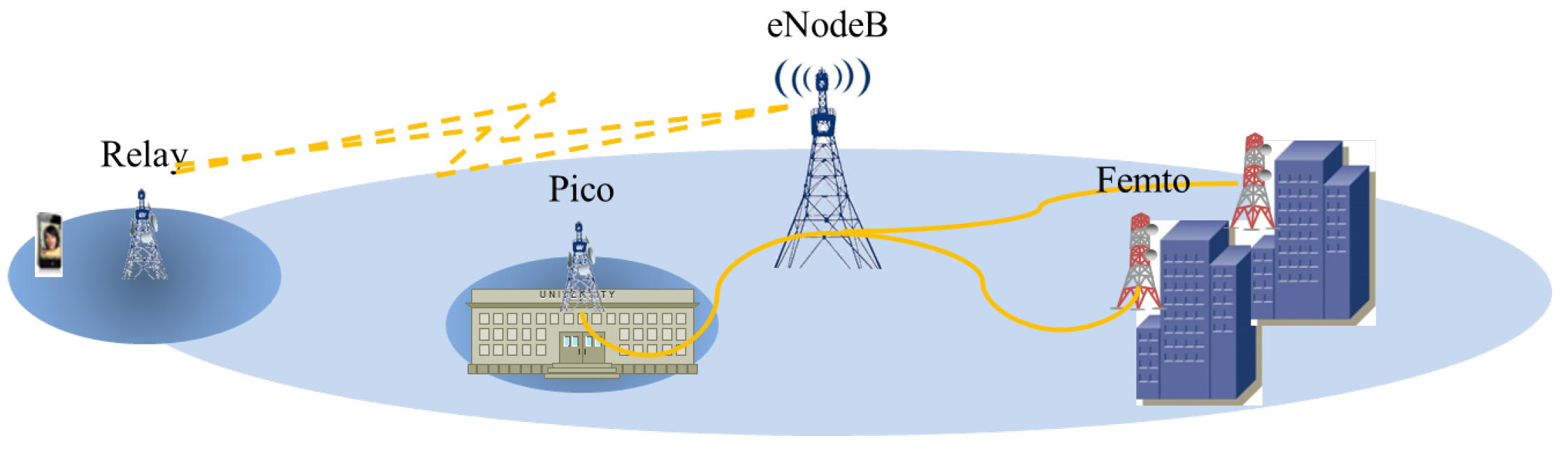
Heterogeneous networks (HetNets) [1,2] are proposed in long-term evolution-advanced (LTE-A) systems by the 3rd Generation Partnership Project (3GPP) to not only meet the rapidly increasing demands of mobile data traffic, but also to reduce the huge energy consumptions caused by data transmissions. A HetNet is a hierarchical network where low-power access points (APs, also named small cell sites [3,4]) are included in a macro-cell, in order to provide highly qualified services. Typical small cell sites include pico, femto, relay and so forth. Femto [5] is mainly for indoor transmissions, while pico [6] is used outdoors in a crowded place, such as a university. Relay [7] is usually built in a remote area far from the macro-cell site (named the Evolved Node B, or eNodeB, in LTE-A HetNet) to extend the coverage of the macro-cell. Figure 1 presents a simple example of a HetNet.

Figure 1. Illustration of a HetNet.

Figure 1. Illustration of a HetNet.

Although HetNets are widely considered as the main trend in the development of mobile communication systems [3], several challenges should be dealt with before implementation in the real world. One of the major challenges is severe intercell interference aggravated by the dense deployment, which crucially affects the performance of HetNets. As a promising measurement to deal with intercell interference, coordinated multiple point (CoMP) [8] techniques are considered to be helpful for HetNets. The basic idea of CoMP techniques is to coordinate coordinated neighboring cells, so that intercell interference can be reduced to a large extent. According to the different ways to cooperate, CoMP techniques are classified into two categories, coordinated scheduling/coordinated beamforming (CS/CB) and joint processing (JP) [9]. CS/CB CoMP makes neighboring cells jointly pre-code according to global channel state information (CSI) to avoid potential interference, while JP CoMP allows neighboring cells to jointly process signals intended for a specific user in the overlapping area. Joint transmission (JT) is a typical JP CoMP technique that requests of cooperating cells to transmit the same data packets to a user independently and simultaneously. In this paper, we take JT CoMP as an example to discuss the performance of CoMP-based HetNet, and the study can also be extended to other CoMP techniques.

To fulfill the requirements of the future mobile networks, CoMP-based HetNets need to provide qualified services as much as possible while maintaining acceptable energy consumption. According to report [10], energy consumption caused by information and communications technology (ICT) has contributed up to 5% of the world-wild power supply at present. To avoid the further increase of energy consumption, mobile networks are required to significantly improve the utility efficiency of power resources. Radio resource management (RRM), which adaptively allocates radio resources, such as frequency and power, according to CSIs, is beneficial for CoMP-based HetNets to enhance the energy efficiency.

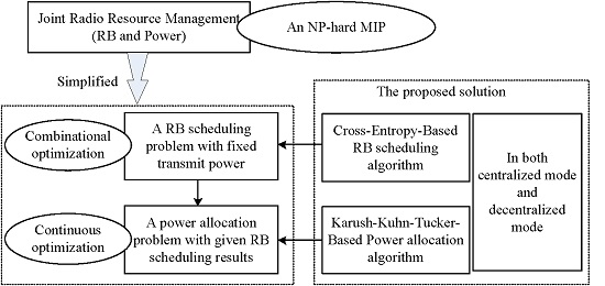
In this paper, we focus on RRM in a CoMP-based HetNet for the purpose of improving the energy efficiency while guaranteeing high data rates, as well as user fairness. An optimization problem aiming at maximizing weighted energy efficiency is formulated, where the weights are employed for maintaining the fairness of users’s data rates. Several crucial constraints in practice are taken into consideration in the formulated problem. Besides the limitation on total power at each transmitter, backhaul links, which connect small cells to the eNodeB for exchanging data and control information, are considered to have restricted capacity. Additionally, the lowest data rate of each transmission is defined, in order to guarantee the quality of transmissions and avoid wasting of energy. Since the formulated problem is unsolvable mixed integer programming (MIP), we separate the whole problem into a scheduling subproblem under the assumption of equal power allocation and a power allocation subproblem with known scheduling results. We first proposed a centralized scheduling algorithm based on cross-entropy (CE) and a corresponding power allocation algorithm. Since centralized algorithms involve numerous calculations, the time delay could be intolerable in a large-scale network. An alternative method to decrease the time delay is to conduct resource allocation in a decentralized way, where calculations are distributed to small cells. For this reason, we also propose modified algorithms that can be used in a decentralized mode.

The rest of this paper is organized as follows. In Section 2, we present the considered system model. Then, the mathematical formulation of the discussed problem is described in Section 3. Section 4 proposes a centralized strategy of resource allocation, which includes a CE-based scheduling algorithm and a power allocation algorithm. Section 5 modifies the proposed algorithms, so that they can be utilized in a decentralized system. Simulation results and relevant analysis are shown in Section 6. At last, we conclude our work in Section 7.

2. System Model

For the sake of simplicity, each independent transmitter, including the macro-cell site and micro-cell sites, is hereby designated as a transmit point (TP) in this paper. We consider a downlink system in a CoMP-based HetNet with M TPs and K user elements (UEs), as shown in Figure 2. $N_{\text{T}}$ and $N_{\text{R}}$ represent the number of antennas on each TP and each UE, respectively. A control unit (CU) is assumed to be located at the center of the network, which is responsible for managing data information, as well as collecting all CSI in this network. TPs are connected to the CU by backhaul links, whereby control information and data packets are delivered to TPs from the CU. Since JT CoMP is employed in our work, there are a large number of data packets that need to be transmitted via backhaul links.

Figure 2. System model.

Figure 2. System model.

The unit of the radio resource in both time and frequency dimensions is referred to as the resource block (RB). As defined in the LTE standard, an RB consists of 12 consecutive subcarriers for a duration of a transmit time interval (TTI) [12]. In this paper, we assume all TPs share the same spectrum bandwidth, which is divided into $N_{\text{RB}}$ RBs in total. Major notations used in this paper are listed in Table 1. Several other important assumptions are considered in our work: channel fading is considered to be quasi-static, so that channel coefficients remain constant per TTI; perfect CSI acknowledgment is assumed at both receivers and transmitters; TPs are synchronized in terms of time, frequency and phase, which is reasonable in the considered system thanks to backhaul connections.

Table 1. Major notations. TP, transmit point; UE, user element; RB, resource block.

Name	Meaning	Name	Meaning
N / K	number of TPs/UEs	${\mathcal{U}}_m$	set of UEs that attaching to TP m
$N_{\text{T}}$ / $N_{\text{R}}$	number of antennas at a TP/UE	$R_k^n$	data rate of UE k on RB n
$\mathcal{M}$	set of all of the TPs	${\overline{R}}_k$	accumulated average data rate of UE k
${\mathcal{M}}_k$	CoMP set of UE k	$p_m^n$	transmit power used at TP m on RB n
${\beta }_{m,k}^n$	index implying the scheduling result	$N_{\text{RB}}$	number of RBs

Table 1. Major notations. TP, transmit point; UE, user element; RB, resource block.

Name	Meaning	Name	Meaning
N / K	number of TPs/UEs	${\mathcal{U}}_m$	set of UEs that attaching to TP m
$N_{\text{T}}$ / $N_{\text{R}}$	number of antennas at a TP/UE	$R_k^n$	data rate of UE k on RB n
$\mathcal{M}$	set of all of the TPs	${\overline{R}}_k$	accumulated average data rate of UE k
${\mathcal{M}}_k$	CoMP set of UE k	$p_m^n$	transmit power used at TP m on RB n
${\beta }_{m,k}^n$	index implying the scheduling result	$N_{\text{RB}}$	number of RBs

2.1. CoMP Set Selection

Ideally, a UE can achieve the optimal data rate if all TPs cooperatively transmit to it. However, the corresponding power consumption and computational complexity are unaffordable. An alternative is to select a CoMP set for the UE according to channel conditions. TPs in the CoMP set can provide the UE a favorable data rate at a much lower cost.

A UE-specific selection of the CoMP set includes three steps:

• TPs broadcast reference signals (RSs) periodically.
• A UE hears the channels and measures them according to the strength of the received RSs. Based on the measurements and a given selection rule, the UE can decide its own CoMP set.
• The UE acknowledges its decision to the CU.

Denote ${\mathcal{M}}_k$ as the CoMP set of UE k and $\mathcal{M}$ as the set including all TPs in the network. UE k decides its ${\mathcal{M}}_k$ following the rule below:

$$\left\{\begin{array}{cc}m\in {\mathcal{M}}_k& m={arg}_{\mathcal{M}}RS\left(\text{the}\text{strongest}\right)\text{or}\\ & RS\left(\text{the}\text{strongest}\right)-RS\left(\text{TP}m\right)\le \Delta \\ m\notin {\mathcal{M}}_k& \text{otherwise}\end{array}\right.$$

(1)

where $RS$ indicates the strength of the reference signal and Δ is a threshold in dB. UE k distinguishes the strongest RS in the first place and adds the corresponding TP to the CoMP set ${\mathcal{M}}_k$. Other TPs will be added to ${\mathcal{M}}_k$ only if the strengths of their RSs are no less than ($RS\left(\text{the}\text{strongest}\right)-\Delta$) dB. As suggested in LTE releases, a rational Δ is in the range of $5-6$ dB [11].

In the case where ${\mathcal{M}}_k$ includes only ‘the strongest TP’, UE k is referred to as a non-CoMP UE in this paper, since no cooperation occurs during downlink transmissions towards it. On the contrary, UE $k^{\prime }$ is referred to as a CoMP UE if its CoMP set ${\mathcal{M}}_{k^{\prime }}$ includes more than one TPs. A CoMP UE is possibly is located at an overlapping area of neighboring cells where intercell interference seriously damages transmissions. To combat interference, TPs in ${\mathcal{M}}_{k^{\prime }}$ are asked to conduct JT CoMP transmissions to UE $k^{\prime }$ for strengthening transmit signals and reducing inter-cell interference.

2.2. Dynamic JT CoMP Transmission

JT CoMP allows TPs in UE’s CoMP set to simultaneously transmit the desired data signal to it. Owing to the spatial separation of the transmit antennas, multiple versions of the desired signal will be received by the UE, which generates extra spatial diversity gain and strengthens the signal. According to information theory [18], the obtained data rate of a JT CoMP transmission to UE k on RB n is given as:

$$R_k^n=blog\left(1+\frac{{\displaystyle \sum _{m\in {\mathcal{M}}_k}}{∥{\mathbf{H}}_{m,k}^2{\mathbf{w}}_m^n∥}^2{p}_m^n}{{\displaystyle \sum _{m^{\prime }\in \mathcal{M}\backslash {\mathcal{M}}_k}}{∥{\mathbf{H}}_{m^{\prime },k}^n{\mathbf{w}}_{m^{\prime }}^2∥}^2{p}_{m^{\prime }}^n+{\sigma }^2}\right)$$

(2)

where ${\mathbf{H}}_{m,k}^n$ is an $N_{\text{R}}\times N_{\text{T}}$ channel matrix between TP m and UE k on the n-th RB. $\mathcal{M}\backslash {\mathcal{M}}_k$ is the complementary of ${\mathcal{M}}_k$ in $\mathcal{M}$, which includes all of the interfering TPs. ${\mathbf{w}}_m^n$ is the precoding vector with dimensions of $N_{\text{T}}\times 1$, which maps data stream $s_m^n$ onto the transmit antennas of TP m, and ${\left({\mathbf{w}}_m^n\right)}^{\text{H}}{\mathbf{w}}_m^n=1$, $E\parallel s_m^n\parallel =1,\forall m,n$. $p_m^n$ is the power used by TP m for transmitting on RB n, and ${\mathbf{n}}_k^n\sim \mathcal{CN}(\mathbf{0},{\sigma }^2{\mathbf{I}}_{N_{\text{R}}})$ is the corresponding complex Gaussian noise vector. b represents the bandwidth of an RB, which is standardized to be 180 kHz in LTE-A systems [12].

Equation (2) implies a static coordinated strategy where TPs in ${\mathcal{M}}_k$ are all required to serve UE k all of the time. However, static strategies are not always optimal due to the time variation of wireless channels. To further improve the network performance, we use a dynamic JT CoMP strategy where a subset of each ${\mathcal{M}}_k$ rather than ${\mathcal{M}}_k$ is adaptively determined to perform JT CoMP transmission. Define a scheduling index ${\beta }_{m,k}^n\in \{0,1\}$ to indicate scheduling results, where ${\beta }_{m,k}^n=1$ means that TP m is chosen to transmit to UE k on the n-th RB. Then, the data rate of a dynamic JT transmission can be given as:

$$R_k^n=blog\left(1+\frac{{\displaystyle \sum _{m=1}^M}{\beta }_{m,k}^n{∥{\mathbf{H}}_{m,k}^2{\mathbf{w}}_m^n∥}^2{p}_m^n}{{\displaystyle \sum _{m^{\prime }=1}^M}\left(1-{\beta }_{m^{\prime },k}^n\right){∥{\mathbf{H}}_{m^{\prime },k}^n{\mathbf{w}}_{m^{\prime }}^2∥}^2{p}_{m^{\prime }}^n+{\sigma }^2}\right)$$

(3)

where ${\sum }_{m=1}^M{\beta }_{m,k}^n\ge 1$.

3. Problem Formulation

In this work, we consider a practical RRM problem in terms of both spectrum and power in a CoMP-based HetNet modeled in the last section. To improve the synthesis performance, the objective involves data rates, power consumption and fairness among UEs at the same time.

The optimal data rate of the network can be achieved if resources are allocated to UEs with better channel conditions, regardless of those in “poor” condition. A side-effect of this scheme is unfavorable fairness of UEs’ data rates. In order to enhance the fairness, we introduce the concept of proportional fairness into the objective of the RRM problem. As in [13], we weighted UE’s data rate by its average data rate determined by:

$${\overline{R}}_k=\alpha {\overline{R}}_k^{\text{before}}+\left(1-\alpha \right)R_k$$

(4)

where $0<\alpha <1$ is the forgetting factor. The introduced weights bring UEs with worse channel conditions more of a possibility to occupy resources and, therefore, increase the UEs’ data rates. The fairness of UEs’ data rates in the network will be improved in this way. To quantify the degree of this fairness, [14] introduces a fairness factor, defined as:

$$F={\left({\displaystyle \sum _{k=1}^K}{R}_k\right)}^2/K{\displaystyle \sum _{k=1}^K}{R}_k^2.$$

(5)

Additionally, for the purpose of conserving energy, energy efficiency should be thoughtfully considered. The energy efficiency is defined by the ratio of the obtained data rate to the total power consumed correspondingly. Combining with proportional fairness principle, the objective of the RRM problem is formulated as,

$${\displaystyle \underset{{\beta }_{m,k}^n,p_m^n}{max}}{\displaystyle \sum _{k=1}^K}{\displaystyle \sum _{n=1}^{N_{\text{RB}}}}\frac{R_k^n}{{\overline{R}}_k}/{\displaystyle \sum _{m=1}^M}{\displaystyle \sum _{n=1}^{N_{\text{RB}}}}{\displaystyle \sum _{k=1}^K}{\beta }_{m,k}^n{p}_m^n$$

(6)

Equation (6) can be considered to maximize the weighted energy efficiency of the network.

In a practical network, system performance is restricted by several factors. In addition to limited transmit power at each TP, the finite capacity of backhaul links defines the upper limit of throughput achieved by a TP during a TTI. Furthermore, to guarantee the quality of transmissions, we impose a threshold to the data rate of each transmission. In summary, the RRM problem of the considered system can be formulated as:

$$\begin{array}{cc}\hfill {\displaystyle \underset{{\beta }_{m,k}^n,p_m^n}{max}}& {\displaystyle \sum _{k=1}^K}{\displaystyle \sum _{n=1}^{N_{\text{RB}}}}\frac{R_k^n}{{\overline{R}}_k}/{\displaystyle \sum _{m=1}^M}{\displaystyle \sum _{n=1}^{N_{\text{RB}}}}{\displaystyle \sum _{k=1}^K}{\beta }_{m,k}^n{p}_m^n\hfill \\ \hfill \text{s.t.}& \text{C1:}0\le p_m^n\le S,\forall m,n\hfill \\ & \text{C2:}{\beta }_{m,k}^n\in \{0,1\},{\displaystyle \sum _{k=1}^K}{\beta }_{m,k}^n\le 1,\forall m,n,k\hfill \\ & \text{C3:}{\displaystyle \sum _{n=1}^{N_{\text{RB}}}}{\displaystyle \sum _{k=1}^K}{\beta }_{m,k}^n{R}_k^n\le C_m,\forall m\hfill \\ & \text{C4:}{R}_k^n\ge R_{\text{thres}},\forall k,n\hfill \end{array}$$

(7)

In Equation (7), C1 shows the power constraint at each transmission where S is the largest transmit power allowed by the system; C2 ensures each index ${\beta }_{m,k}^n$ to be a bit number, so that a TP can serve no more than one UE on each RB; C3 demonstrates the constrained throughput of a TP caused by the limited capacity of backhaul connections to the CU, where $C_m$ represents the capacity of the backhaul link connecting TP m and the CU; and C4 guarantees the data rate of each ongoing transmission, where $R_{\text{thres}}$ is the given threshold of the data rate.

4. Centralized Algorithm

Since the problem in Equation (7) is NP-hard, it is unpractical to achieve the optimal solution. An alternative method is to consider the problem as a combination of a scheduling problem under the consumption of equal power allocation and a power allocation problem with a given scheduling result. In this way, an approximated solution of the problem can be obtained in polynomial time.

In the rest of this section, we propose a heuristic algorithm based on CE for RB scheduling with equal transmit power at the first place. Then, a Karush-Kuhn-Tucker-method to solve the power allocation problem is presented. The algorithm involving both RB scheduling and power allocation proposed in this section is centralized, which means that the resource allocation is operated at the CU with global CSI. The centralized algorithm is capable of achieving a favorable system performance, but it requires significant computational effort of the CU. In the next section, we also propose a decentralized algorithm of resource allocation with lower complexity and delay of computation, which leads to decreased performance unavoidably.

4.1. CE-Based Scheduling Algorithm

The objective of the considered RB scheduling problem becomes

$${\displaystyle \underset{{\beta }_{m,k}^n,p_m^n}{max}}{\displaystyle \sum _{k=1}^K}{\displaystyle \sum _{n=1}^{N_{\text{RB}}}}\frac{R_k^n}{{\overline{R}}_k}/{\displaystyle \sum _{m=1}^M}{\displaystyle \sum _{n=1}^{N_{\text{RB}}}}{\displaystyle \sum _{k=1}^K}{\beta }_{m,k}^{n}S$$

(8)

where S is the fixed transmit power. The objective is constrained by C2, C3 and C4 in Equation (7). We first propose a CE-based algorithm to solve the RB scheduling problem described above.

The CE method is a typical heuristic algorithm to estimate the probabilities of rare events in complex stochastic networks [15] and to deal with linear programming. The basic idea of the CE method is to generate sufficient samples under a given strategy and then update the generating strategy according to samples. After iteratively repeating this procedure, generated samples will converge to the optimal solution. The proposed CE-based scheduling algorithm follows three major stages, including initialization, iteration and a complementary stage to close unfavorable transmissions, as shown in Figure 3.

Figure 3. The major principle of the CE method.

Figure 3. The major principle of the CE method.

4.1.1. Initialization

Let ${\mathbf{X}}^m=[x_{\left(1\right)}^m,...,x_{\left(n\right)}^m,...,x_{\left(N_{\text{RB}}\right)}^m]$ ($x_{\left(n\right)}^m\in \left[0,{\mathcal{U}}_m\right]$) denote a sample generated according to a given probability, which presents a possible scheduling result of TP m. $x_{\left(n\right)}^m=0$ means that no transmission is scheduled on RB n of TP m. Otherwise, $x_{\left(n\right)}^m$ is the ID of the scheduled UE. In the CE method, the scheduling problem is regarded as a stochastic procedure. The distribution of $x_{\left(n\right)}^m$ is denoted by ${\mathbf{q}}^{m,n}=[q_0^{m,n},q_1^{m,n},...,q_u^{m,n},...,q_{|{\mathcal{U}}_m|}^{m,n}]$, where $q_u^{m,n}=\mathbb{P}\{x_{\left(n\right)}^m=u\},u\in [0,{\mathcal{U}}_m]$. Obviously, $q_u^{m,n}$ has the attributes of $0\le q_u^{m,n}\le 1$ ($\forall u,m,n$) and ${\sum }_{u\in [0,{\mathcal{U}}_m]}{q}_u^{m,n}=1$ ($\forall m,n$).

For the sake of accelerating convergence, we design the initial probability distribution according to estimated data rates. We first defined $\mathbb{P}\{x_{\left(n\right)}^m=0\}={\text{Pr}}_0$ where ${\mathrm{Pr}}_0$ is a given value. This probability gives an opportunity to TP m for scheduling no transmission on RB n. For each $u\in {\mathcal{U}}_m$, the data rate $R_u^n$ is estimated based on the fixed JT CoMP transmission, as given by (2), at the initialization stage. As suggested by C4 in (7), the transmission is considered to be unqualified if $R_u^n<R_{\text{thres}}$. To save energy, the proposed algorithm sets the corresponding probability to be zero, i.e., $q_u^{m,n}=0$. For the rest of the optional UEs, the probability is defined as $q_u^{m,n}=\left(R_u^n/R_{\text{tot}}^m\right)\times \left(1-{\text{Pr}}_0\right)$, where $R_{\text{tot}}$ indicates the sum data rate of all possible qualified transmissions, defined as:

$$R_{\text{tot}}^m={\displaystyle \sum _{\begin{array}{c}k\in {\mathcal{U}}_m,\\ R_k^n\ge R_{\text{thres}}\end{array}}}{R}_k^n$$

(9)

Summarily, the initial distribution of $x_{\left(n\right)}^m$ is:

$$q_u^{m,n}=\left\{\begin{array}{cc}{\text{Pr}}_0,\hfill & u=0\hfill \\ \left(1-{\text{Pr}}_0\right)\times R_u^n/R_{\text{tot}}^m,\hfill & u\in {\mathcal{U}}_m,\text{and}{R}_u^n\ge R_{\text{thres}}\hfill \\ 0,\hfill & u\in {\mathcal{U}}_m,\text{and}{R}_u^n<R_{\text{thres}}\hfill \end{array}\right.$$

(10)

4.1.2. Iteration

Each iteration of the proposed algorithm includes three steps. First, the algorithm generates adequate samples according to a given strategy. Then, it is necessary to exclude those samples that do not satisfy the constraints and to select “good” samples for the next stage. At last, the probability distribution needs to be updated according to the selected samples, so that “better” samples will be generated in the next iteration. After sufficient iterations, the algorithm gradually approaches the optimal solution.

Let $N_{\text{SAM}}$ denote the number of samples generated in each iteration for each TP and ${\mathbf{X}}_1^m,···,{\mathbf{X}}_i^m,···,{\mathbf{X}}_{N_{\text{SAM}}}^m$ denote the corresponding samples, where ${\mathbf{X}}_i^m=[x_{i\left(1\right)}^m,···,x_{i\left(n\right)}^m,···,x_{i\left(N_{\text{RB}}\right)}^m]$. Each sample can map into a scheduling index set {${\beta }_{m,k}^n,\forall k,n$}, and leads to a weighted energy efficiency of TP m given as:

$$f_m\left({\mathbf{X}}_i^m\right)={\displaystyle \sum _{n=1}^{N_{\text{RB}}}}\frac{R_{x_{i\left(n\right)}^m}^n}{{\overline{R}}_{x_{i\left(n\right)}^m}}/{\displaystyle \sum _{n=1,x_i^m\left(n\right)\ne 0}^{N_{\text{RB}}}}S$$

(11)

where ${\sum }_{n=1,x_i^m\left(n\right)\ne 0}^{N_{\text{RB}}}S$ represents the total power consumption at TP m according to sample ${\mathbf{X}}_i^m$. The sum data rate of TP m can be estimated as $R_m\left({\mathbf{X}}_i^m\right)={\sum }_{n=1}^{N_{\text{RB}}}{R}_{x_{i\left(n\right)}^n}^n$.

A qualified sample should satisfy two requirements. First, the sum data rate $R_m$ cannot exceed the backhaul capacity of TP m. Therefore, those samples lead to overlarge sum data rates, i.e., $R_m\left({\mathbf{X}}_i^m\right)>C_m$, will be removed. Second, the value of $f_m\left({\mathbf{X}}_i^m\right)$ should be high enough. Samples whose weighted energy efficiency $f_m\left({\mathbf{X}}_i^m\right)<f_{\text{thres}}^{\left(t\right)}$ will also be removed, where $f_{\text{thres}}^{\left(t\right)}$ is a threshold that increases after each iteration until it converges. Consequently, $N_{\text{IM}}$ $(N_{\text{IM}}\le N_{\text{SAM}})$ qualified samples are left for updating the generation probability. Without loss of generality, qualified samples are denoted as ${\mathbf{X}}_j^m\left(1\le j\le N_{\text{IM}}\right)$.

At the last stage of an iteration, probability distributions are updated on the basis of qualified samples in order to generate better samples in the next iteration. The updated possibility $\mathbb{P}\{x_{\left(n\right)}^m=u\}$ is:

$$q_u^{m,n}=N\left(x_{j\left(n\right)}^m=u\right)/N_{\text{IM}}$$

(12)

where $N\left(x_{j\left(n\right)}^m=u\right)$ represents the number of times that UE u appears in $N_{\text{IM}}$ samples on the n-th RB.

The proposed iteration algorithm is summarized as Algorithm 1.

Algorithm 1 Iteration in the CE-based scheduling algorithm.

1: $f_{\text{max}}=f_{\text{max}\_\text{pre}}=0$; $counter=1$; 2: while $counter\le N_{\text{SAM}}$ do 3:   Generate samples ${\mathbf{X}}^m$ according to the distribution ${\mathbf{q}}^{m,n}$. 4:   Calculate utility function of ${\mathbf{X}}_i^m$, i.e., $f\left({\mathbf{X}}_i^m\right)$, according to (11). 5:   Calculate the sum data rate of ${\mathbf{X}}^m$, i.e., $R_m\left({\mathbf{X}}^m\right)={\sum }_{k\in {\mathcal{U}}_m}{R}_k^n$. 6:   if $f\left({\mathbf{X}}^m\right)<f_{\text{thres}}^{\left(t\right)}$ then 7:       CONTINUE; 8:   end if 9:   if $R_m\left({\mathbf{X}}^m\right)>C_m$ then 10:       CONTINUE; 11:   end if 12:   ${\mathbf{X}}_{counter}^m={\mathbf{X}}^m$ 13:   $counter=counter+1$ 14: end while 15: for $i=1\text{to}{N}_{\text{SAM}}$ do 16:   Calculate $f\left({\mathbf{X}}_i^m\right)$ according to (11). 17: end for 18: Sort samples in a descending order in terms of $f\left({\mathbf{X}}_i^m\right)$. Denote the consequence by ${\widehat{\mathbf{X}}}_1^m,{\widehat{\mathbf{X}}}_2^m,·,{\widehat{\mathbf{X}}}_{\text{SAM}}^m$ 19: Calculate $N_{\text{IM}}=⌈(1-\rho )N_{\text{SAM}}⌉$, and let $f_{\text{thres}}^{(t+1)}=f\left({\widehat{\mathbf{X}}}_{N_{\text{IM}}^m}\right)$ 20: if $f\left({\widehat{\mathbf{X}}}_1^m\right)>f_{max}$ then 21:   ${\mathbf{X}}_{\text{out}}^m={\widehat{\mathbf{X}}}_1^m$, $f_{\text{max}\_\text{pre}}=f_{\text{max}}$, $f_{\text{max}}=f\left({\widehat{\mathbf{X}}}_1^m\right)$ 22: end if 23: Update ${\mathbf{q}}^{m,n}$ according to (12) 24: Map ${\mathbf{X}}_{\text{out}}^m$ into ${\beta }_{m,k}^n$, and recalculate $R_k^n$ according to (3)

4.1.3. Removing Unqualified Transmissions

The algorithm proposed above cannot ensure that the data rate of each transmission is as high as the given threshold $R_{\text{thres}}$. Since we put our purpose on improving energy efficiency, it is reasonable to close those transmissions that are estimated to be unqualified.

Algorithm 2 summaries the entire RB scheduling algorithm proposed above.

Algorithm 2 Centralized RB scheduling algorithm.

1: Calculate $R_k^n$ according to Equation (2). 2: Initialize probability distribution ${\mathbf{q}}^m(m=1,···,M)$ according to Equation (10). 3: for $t=1:t_{\text{max}}$ do 4:   for $m=1:M$ do 5:       Process Algorithm 1, and output ${\mathbf{X}}_{\mathbf{\text{out}}}^m,(m=1,···,M)$ 6:   end for 7:   Map obtained ${\mathbf{X}}_{\text{out}}^m$ into $\{{\beta }_{m,k}^n\}$. 8:   Update $R_k^n$ according to Equation (3), and obtain $\{{\beta }_{m,k}^n\}$. 9:   if All of the elements in ${\mathbf{q}}^m(m=1,·,·,·,M)$ converge then 10:       Output ${\mathbf{X}}_{\text{out}}$ 11:       BREAK 12:   end if 13: end for 14: Map obtained ${\mathbf{X}}_{\text{out}}^m$ into $\{{\beta }_{m,k}^n\}$. 15: for $n=1:N_{\text{RB}}$ do 16:   for $u=1:K$ do 17:       if $R_k^n<R_{\text{thres}}$ then 18:             Let the corresponding ${\beta }_{m,u}^n=0$. 19:       end if 20:   end for 21: end for

4.2. Power Allocation Algorithm

With the obtained RB scheduling result, the power allocation problem can be given as:

$$\begin{array}{cc}\hfill {\displaystyle \underset{{\beta }_{m,k}^n,p_m^n}{max}}& {\displaystyle \sum _{k=1}^K}{\displaystyle \sum _{n=1}^{N_{\text{RB}}}}\frac{R_k^n}{{\overline{R}}_k}/{\displaystyle \sum _{m=1}^M}{\displaystyle \sum _{n=1}^{N_{\text{RB}}}}{\displaystyle \sum _{k=1}^K}{\beta }_{m,k}^n{p}_m^n\hfill \\ \hfill \text{s.t.}& \text{C1:}0\le p_m^n\le S,\forall m,n\hfill \\ & \text{C3:}{\displaystyle \sum _{n=1}^{N_{\text{RB}}}}{\displaystyle \sum _{k=1}^K}{\beta }_{m,k}^n{R}_k^n\le C_m,\forall m\hfill \\ & \text{C4:}{R}_k^n\ge R_{\text{thres}},\forall k,n\hfill \end{array}$$

(13)

The objective function in (13) is a well-known non-convex function for which the optimal solution does not exist. In this work, we use an analytical method on the base of the KKT-condition to approach a local optimal solution of power allocation.

A solution of Equation (13) can be achieved by solving its dual function in terms of backhaul and data rate constraints given as:

$$\begin{array}{cc}\hfill {\displaystyle \underset{p_m^n}{max}}& {\displaystyle \sum _{n=1}^{N_{\text{RB}}}}\left({\displaystyle \sum _{k=1}^K}\frac{R_k^n}{{\overline{R}}_k}/{\displaystyle \sum _{m=1}^M}{p}_m^n\right)-{\displaystyle \sum _{m=1}^M}{\lambda }_m\left({\displaystyle \sum _{n=1}^{N_{\text{RB}}}}{\displaystyle \sum _{k=1}^K}{\beta }_{m,k}^n{R}_k^n-C_m\right)+{\displaystyle \sum _{n=1}^{N_{\text{RB}}}}{\displaystyle \sum _{k=1}^K}{\mu }_{n,k}\left(R_k^n-R_{\text{thres}}\right)\hfill \\ \hfill \text{s}.t.& 0\le p_m^n\le S,\forall m,n\hfill \end{array}$$

(14)

where {${\lambda }_m$, $\forall m$} and {${\mu }_{n,k}$, $\forall n,k$} are non-negative Lagrangian multipliers. However, the dual function given above is still hard to solve, since it involves too many variables ($M{N}_{\text{RB}}$ variables and Lagrangian multipliers). To further simplify the problem, we intend to decompose Equation (14) into independent subproblems with fewer variables.

Let ${\beta }_m={\sum }_{n=1}^{N_{\text{RB}}}{\sum }_{k=1}^K{\beta }_{m,k}^n$. ${\beta }_m=0$ indicate the situation where no transmission is scheduled for TP m. This is unreasonable in the high-loading network we considered. Thus, we suppose that ${\beta }_m\ne 0$; then $C_m$ can be rewritten as:

$$C_m={\displaystyle \sum _{n=1}^{N_{\text{RB}}}}{\displaystyle \sum _{k=1}^K}{\beta }_{m,k}^n\frac{C_m}{{\displaystyle \sum _{n=1}^{N_{\text{RB}}}}{\displaystyle \sum _{k=1}^K}{\beta }_{m,k}^n}={\displaystyle \sum _{n=1}^{N_{\text{RB}}}}{\displaystyle \sum _{k=1}^K}{\beta }_{m,k}^n\frac{C_m}{{\beta }_m}$$

(15)

After substituting (15) into (14), the problem can be decomposed into $N_{\text{RB}}$ independent subproblems, where each subproblem is given as:

$$\begin{array}{cc}\hfill {\displaystyle \underset{p_m^n}{max}}& {\displaystyle \sum _{k=1}^K}\frac{R_k^n}{{\overline{R}}_k}/{\displaystyle \sum _{m=1}^M}{p}_m^n-{\displaystyle \sum _{k=1}^K}{\displaystyle \sum _{m=1}^M}{\lambda }_m{\beta }_{m,k}^n\left(R_k^n-\frac{C_m}{{\beta }_m}\right)+{\displaystyle \sum _{k=1}^K}{\mu }_{n,k}\left(R_k^n-R_{\text{thres}}\right)\hfill \\ \hfill \text{s.t.}& 0\le p_m^n\le S,\forall m\hfill \end{array}$$

(16)

Each subproblem in Equation (16) involves M variables with Lagrangian multipliers only and can be solved independently on each RB. The computational complexity is significantly cut in this way. In the rest of this subsection, we propose an iterative method to address each subproblem.

Let $f_n(p_m^n,{\lambda }_m,{\mu }_{n,k})$ denote the objective function of Equation (16). Take the first order derivative in terms of $p_m^n$, and make it equal to zero; then, a possible value of power allocation, denoted by ${\widehat{p}}_m^n$, can be obtained as follows,

$${\widehat{p}}_m^n=\left\{\frac{\left(\frac{1}{{\overline{R}}_{k^{*}}·p_{\text{t}ot}^n}-{\displaystyle \sum _{m=1}^M}{\lambda }_m·{\beta }_{m,k^{*}}^n+{\mu }_{n,k^{*}}\right)·b{\displaystyle \sum _{m\in \mathcal{M}}}{\beta }_{m,k^{*}}^n{\parallel {\mathbf{H}}_{m,k^{*}}^n{\mathbf{w}}_m^n\parallel }^2}{\frac{1}{{\left(p_{\text{t}ot}^n\right)}^2}·{\displaystyle \sum _{k=1}^K}\frac{R_k^n}{{\overline{R}}_k}-{\displaystyle \sum _{k=1;k\ne k^{*}}^K}\left(\frac{1}{{\overline{R}}_k·p_{\text{t}ot}^n}-{\displaystyle \sum _{m=1}^M}{\lambda }_m·{\beta }_{m,k}^n+{\mu }_{n,k}\right)·\frac{\partial R_k^n}{\partial p_m^n}}-A_m^n\right\}\times \frac{1}{\parallel {\mathbf{H}}_{m,k^{*}}^n{\mathbf{w}}_m^n{\parallel }^2}$$

(17)

where $p_{tot}^n={\sum }_{m=1}^M{p}_m^n$ and $k^{*}$ is the UE scheduled on RB n of TP m, i.e., ${\beta }_{m,k^{*}}^n=1$. The derivative $\partial R_k^n/\phantom{\partial R_k^n\partial p_m^n}\partial p_m^n$ and $A_m^n$ are given by:

$$\frac{\partial R_k^n}{\partial p_m^n}=-\frac{b{\left({\gamma }_k^n\right)}^2}{1+{\gamma }_k^n}\frac{{∥{\mathbf{H}}_{m,k}^n{\mathbf{w}}_m^n∥}^2}{{\displaystyle \sum _{m^{\prime }\in \mathcal{M}}}{\beta }_{m^{\prime },k}^n{∥{\mathbf{H}}_{m^{\prime },k}^n{\mathbf{w}}_{m^{\prime }}^n∥}^2{p}_{m^{\prime }}^n},\forall k\ne k^{*}$$

(18)

and:

$$A_m^n={\displaystyle \sum _{m^{\prime }\in \mathcal{M}\backslash \{m\}}}{\parallel {\mathbf{H}}_{m^{\prime },k^{*}}^n{\mathbf{w}}_{m^{\prime }}^n\parallel }^2{p}_{m^{\prime }}^2+{\sigma }^2$$

(19)

respectively.

The obtained ${\widehat{p}}_m^n$ above may not be in the range of $[0,S]$. Therefore, the real power allocation needs to be adjusted following the rule given by:

$$p_m^{n\left(t\right)}=max\left\{min\left\{{\widehat{p}}_m^n,S\right\},0\right\}$$

(20)

where t indicates the times of the iteration.

Lagrangian multipliers can be updated in each iteration by the sub-gradient method [16] as follows,

$$\begin{array}{c}{\lambda }_m^{(t+1)}=max\left\{{\lambda }_m^{\left(t\right)}-v_{\lambda }^{\left(t\right)}\left({\displaystyle \sum _{n=1}^{N_{\text{RB}}}}{\displaystyle \sum _{k=1}^K}{\beta }_{m,k}^n{R}_k^n-C_m\right),0\right\}\hfill \\ {\mu }_{n,k}^{(t+1)}=max\left\{{\mu }_{n,k}^{\left(t\right)}-v_{\mu }^{\left(t\right)}\left(R_{\text{thres}}-R_k^n\right),0\right\}\hfill \end{array}$$

(21)

where $v_{\lambda }^{\left(t\right)}$ and $v_{\mu }^{\left(t\right)}$ are the step sizes used in the current iteration for updating ${\lambda }_m$ and ${\mu }_{n,k}$.

5. Decentralized Algorithm

The centralized strategy of resource allocation proposed above is processed on the CU with the global CSI at the beginning of each TTI. It is possible that the time delay caused by processing is too long to guarantee the effectiveness of a large-scale system involving numerous TPs and UEs. An alternative method for shortening the time delay is a decentralized strategy that distributes calculations to each TP instead of the CU. Under a decentralized strategy, global CSIs are shared between TPs at the first place. Then, the resource allocation is processed at each TP independently and simultaneously, according to the known CSIs and a given strategy. In this way, the time delay of processing can be significantly decreased, even in a large-scale network. However, due to the lack of knowledge about the scheduling results of other TPs, the accuracy of the decentralized one is unavoidably worse than the centralized one.

In this section, we propose a decentralized strategy with the similar CE-based scheduling and KKT-based power allocation to the centralized proposed above. Simulation results presented in Section 6 will prove that the decline of system performance under the proposed decentralized strategy is acceptable.

5.1. Decentralized RB Scheduling Algorithm

A decentralized RB scheduling algorithm based on the CE method is proposed in this subsection. The same as the centralized one proposed in Subsection 4.1, the decentralized scheduling algorithm initializes the probability distribution ${\mathbf{q}}^m$ at the first place. Then, the iteration procedure is processed to obtain RB scheduling results. It should be noticed that the decentralized strategy cannot accurately estimate data rates of ongoing transmissions due to the lack of information about the scheduling results of other TPs. Therefore, the decentralized scheduling algorithm deletes the procedure of removing unqualified transmissions (as described in Section 4.1.3). In the simulation, we consider unqualified transmissions as failures, which waste energy and contribute nothing to the data rates of the system. Algorithm 3 summarizes the decentralized RB scheduling based on the CE method.

Algorithm 3 Decentralized RB scheduling algorithm.

1: Calculate $R_k^n$ according to Equation (2). 2: Initialize probability distribution ${\mathbf{q}}^m(m=1,···,M)$ according to Equation (10). 3: for $t=1:t_{\text{max}}$ do 4:   Process Algorithm 1, and output ${\mathbf{X}}_{\text{out}}^m,(m=1,···,M)$ 5:   if All of the elements in ${\mathbf{q}}^m=[q^{m,n},\forall n]$ converge then 6:       Output ${\mathbf{X}}_{\text{out}}$ 7:       BREAK 8:   end if 9: end for 10: Map the obtained ${\mathbf{X}}_{\text{out}}^m$ into $\{{\beta }_{m,k}^n\}$.

5.2. Power Allocation Algorithm

In this subsection, we modify the power allocation algorithm proposed in Subsection 4.2 to be decentralized, so that it can be processed at each TP independently and simultaneously. The individual power allocation problem of each TP is given by:

$$\begin{array}{cc}\hfill max& {\displaystyle \sum _{k=1}^K}{\displaystyle \sum _{n=1}^{N_{\text{RB}}}}{\beta }_{m,k}^n\frac{R_k^n}{{\overline{R}}_k}/{\displaystyle \sum _{k=1}^K}{\displaystyle \sum _{n=1}^{N_{\text{RB}}}}{\beta }_{m,k}^n{p}_m^n\hfill \\ \hfill \text{s.t.}& \text{C1:}0\le p_m^n\le S,\forall n\hfill \\ & \text{C3:}{\displaystyle \sum _{n=1}^{N_{\text{RB}}}}{\displaystyle \sum _{k=1}^K}{\beta }_{m,k}^n{R}_k^n\le C_m\hfill \\ & \text{C4:}{R}_k^n\ge R_{\text{thres}},\forall n,k\in {\mathcal{U}}_m\hfill \end{array}$$

(22)

As in Subsection 4.2, we constitute and solve the dual function of Equation (22), instead of solving it directly. The dual function in terms of constraints C3 and C4 is given as:

$$\begin{array}{cc}\hfill {\displaystyle \underset{p_m^n}{max}}& {\displaystyle \sum _{n=1}^{N_{\text{RB}}}}\left({\displaystyle \sum _{k=1}^K}{\beta }_{m,k}^n\frac{R_k^n}{{\overline{R}}_k}/{\displaystyle \sum _{k=1}^K}{\beta }_{m,k}^n{p}_m^n\right)-{\lambda }_m\left({\displaystyle \sum _{n=1}^{N_{\text{RB}}}}{\displaystyle \sum _{k=1}^K}{\beta }_{m,k}^n{R}_k^n-C_m\right)\hfill \\ & +{\displaystyle \sum _{n=1}^{N_{\text{RB}}}}{\displaystyle \sum _{k=1}^K}{\mu }_{n,k}{\beta }_{m,k}^n\left(R_k^n-R_{\text{thres}}\right)\hfill \\ \hfill \text{s.t.}& 0\le p_m^n\le S,\forall n\hfill \end{array}$$

(23)

Substituting Equation (15) into Equation (23), we can decompose the power allocation problem into $N_{\text{RB}}$ independent subproblems. Let $f_{m,n}$ denote the objective of the subproblem on RB n of TP m, which is given as:

$$f_{m,n}={\displaystyle \sum _{k=1}^K}{\beta }_{m,k}^n\frac{R_k^n}{{\overline{R}}_k}/{\displaystyle \sum _{k=1}^K}{\beta }_{m,k}^n{p}_m^n-{\displaystyle \sum _{k=1}^K}{\lambda }_m{\beta }_{m,k}^n\left(R_k^n-\frac{C_m}{{\beta }_m}\right)+{\displaystyle \sum _{k=1}^K}{\mu }_{n,k}{\beta }_{m,k}^n\left(R_k^n-R_{\text{thres}}\right)$$

(24)

${\displaystyle \sum _{k=1}^K}{\beta }_{m,k}^n=0$ means that TP m does not schedule any transmissions on RB n. In this case, power allocation is not required, i.e., $p_m^n=0$. In the case where ${\displaystyle \sum _{k=1}^K}{\beta }_{m,k}^n=1$, transmit power $p_m^n$ can be obtained by an iterative method proposed in the rest of this subsection.

Let $k^{*}$ denote the UE of TP m scheduled on RB n (i.e., ${\sum }_{k=1}^K{\beta }_{m,k}^n={\beta }_{m,k^{*}}^n=1$). Taking the first order derivative of $f_{m,n}$ with respect to $p_m^n$, we obtain:

$$\frac{\partial f_{m,n}}{\partial p_m^n}=\left(\frac{1}{{\overline{R}}_{k^{*}}{p}_m^n}-{\lambda }_m+{\mu }_{n,k^{*}}\right)\frac{\partial R_{k^{*}}^n}{\partial p_m^n}-\frac{R_{k^{*}}^n}{{\overline{R}}_{k^{*}}{\left(p_m^n\right)}^2}$$

(25)

where:

$$\frac{\partial R_{k^{*}}^n}{p_m^n}=\frac{b{\displaystyle \sum _{m\in \mathcal{M}}}{\beta }_{m,k^{*}}^n{∥{\mathbf{H}}_{m,k^{*}}^n{\mathbf{w}}_m^n∥}^2}{{∥{\mathbf{H}}_{m,k^{*}}^n{\mathbf{w}}_m^n∥}^2{p}_m^n+{\displaystyle \sum _{m^{\prime }\in \mathcal{M}\backslash \{m\}}}{∥{\mathbf{H}}_{m^{\prime },k^{*}}^n{\mathbf{w}}_{m^{\prime }}^n∥}^2{p}_{m^{\prime }}^n+{\sigma }^2}$$

(26)

Let $\partial f_n/\partial p_m^n=0$. An expression of $p_m^n$ in the t-th iteration can be obtained by solving the equation, which is given as:

$$p_m^{n\left(t\right)}=\sqrt{\frac{R_{k^{*}}^n}{{\overline{R}}_{k^{*}}}}\times \sqrt{\frac{{∥{\mathbf{H}}_{m,k^{*}}^n{\mathbf{w}}_m^n∥}^2{p}_m^{n\left(t\right)}+{\displaystyle \sum _{\begin{array}{c}{m}^{\prime }\in \mathcal{M}\\ m^{\prime }\ne m\end{array}}}{∥{\mathbf{H}}_{m^{\prime },k^{*}}^n{\mathbf{w}}_{m^{\prime }}^n∥}^2{p}_{m^{\prime }}^{n\left(t\right)}+{\sigma }^2}{b{∥{\mathbf{H}}_{m,k^{*}}^n{\mathbf{w}}_m^n∥}^2\left(\frac{1}{{\overline{R}}_{k^{*}}{p}_m^{n\left(t\right)}}-\left({\lambda }_m-{\mu }_{n,k^{*}}\right)\right)}}$$

(27)

where multipliers ${\lambda }_m$ and ${\mu }_{n,k^{*}}$ should be updated according to Equation (21). A suboptimal $p_m^n$ can be approached after sufficient iterations.

6. Simulation Results

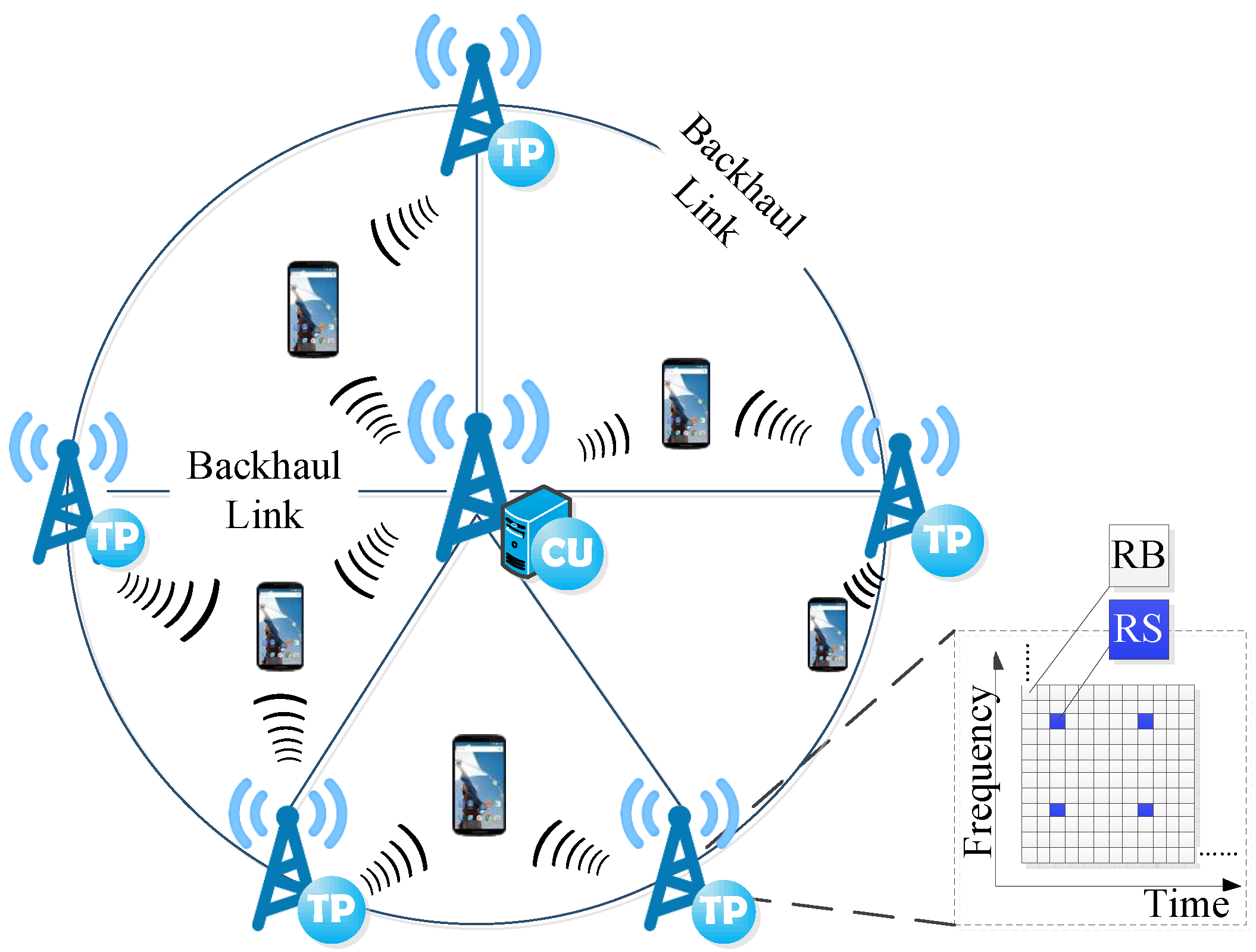
We consider a HetNet downlink system with 37 TPs, where only 19 TPs of these conduct actual communications to UEs, and the others wrap them around to produce virtual interference. The radius of each small cell is 250 m, since a dense deployment is considered. The system includes 100 RBs, each of which is under a bandwidth of 180 kHz. Therefore, the overall bandwidth of the system is 18 MHz. Additionally, $2\times 2$ MIMO links are created using the space channel model (SCM) [17]. Each simulation lasts 20 TTIs, where a TTI is 1 ms. Important parameters used in the simulation are listed in Table 2.

Table 2. Parameters in the simulation.

Parameters	Value
Layout of cells	37 hexagon cells; wrap-around used
Radius of cells	250 m
Central frequency	2 GHz
$N_{\text{RB}}$, number of RBs	100
$S_m$, limit of transmit power	20 Watt
$N_{\mathrm{T}}\times N_{\mathrm{R}}$	2 × 2
number of TTI / TTI	20 /1 ms
α	0.1
Channel model	SCM (path loss + shadowing + MIMO fading)
Minimal distance (TP and UE)	35 m
Height of transmit/receive antenna	35 m/1.5 m
Penetration loss	20 dB
Traffic model	full buffer
Speed of UE	10 m/s

Table 2. Parameters in the simulation.

Parameters	Value
Layout of cells	37 hexagon cells; wrap-around used
Radius of cells	250 m
Central frequency	2 GHz
$N_{\text{RB}}$, number of RBs	100
$S_m$, limit of transmit power	20 Watt
$N_{\mathrm{T}}\times N_{\mathrm{R}}$	2 × 2
number of TTI / TTI	20 /1 ms
α	0.1
Channel model	SCM (path loss + shadowing + MIMO fading)
Minimal distance (TP and UE)	35 m
Height of transmit/receive antenna	35 m/1.5 m
Penetration loss	20 dB
Traffic model	full buffer
Speed of UE	10 m/s

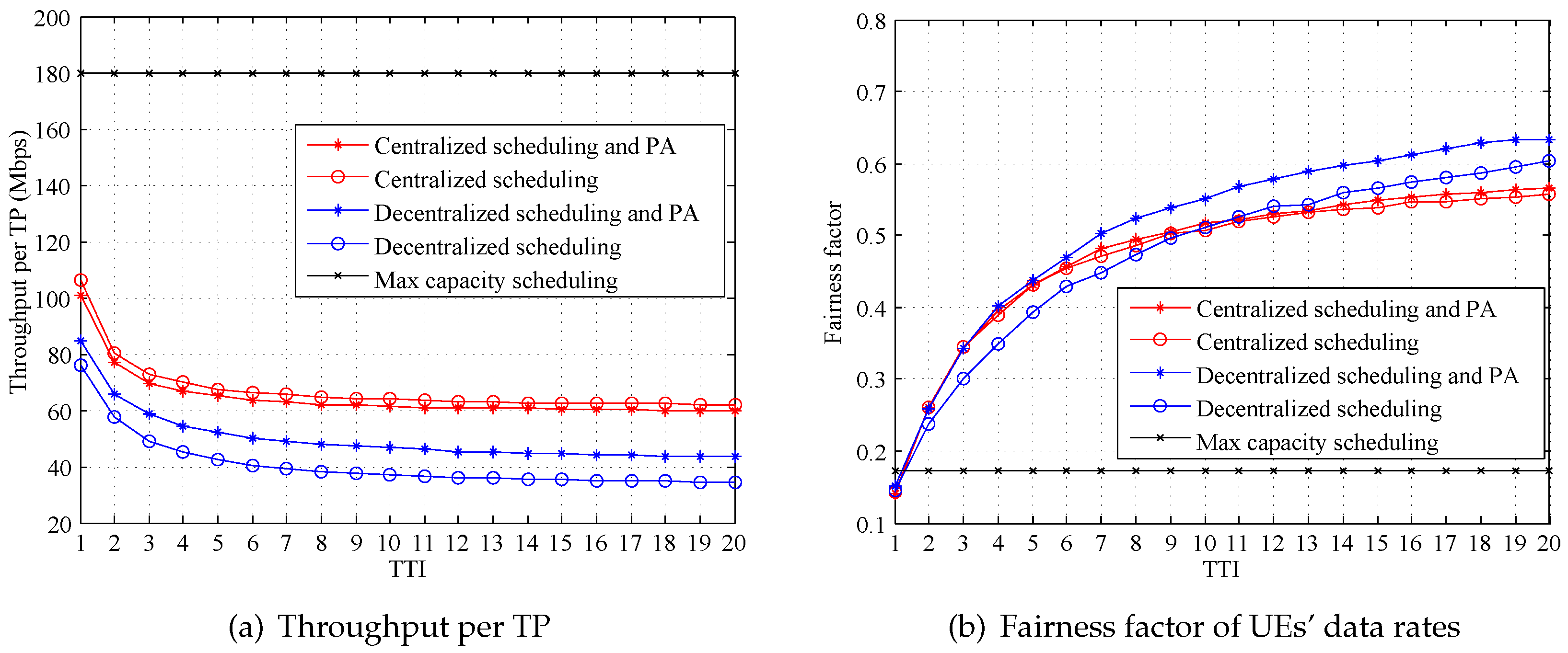
The simulation is carried out to prove the proposed algorithms effectiveness. A greedy algorithm, named max capacity, is also simulated as a benchmark. The max capacity algorithm tends to allocate resources to UEs with good channel conditions, in order to reach the optimal throughput of the network. In this way, UEs with worse channel conditions may no chance to communicate. Therefore, the fairness of the max capacity algorithm is unfavorable. Figure 4 and Figure 5 compare the performances of the max capacity algorithm to that of the proposed one.

Figure 4 demonstrates the average throughput per TP and fairness factor (as defined by Equation (5)) of the system under different resource allocation algorithms, when the transmit power of each TP is 20 Watts. It is obvious that max capacity algorithm achieves an outstanding throughput and a much worse fairness factor than the proposed one. The future mobile communication system targets to provide not only high throughput of the network, but also quality service to every UE. Therefore, the max capacity is no longer appropriate. The proposed algorithms have much better fairness factors. 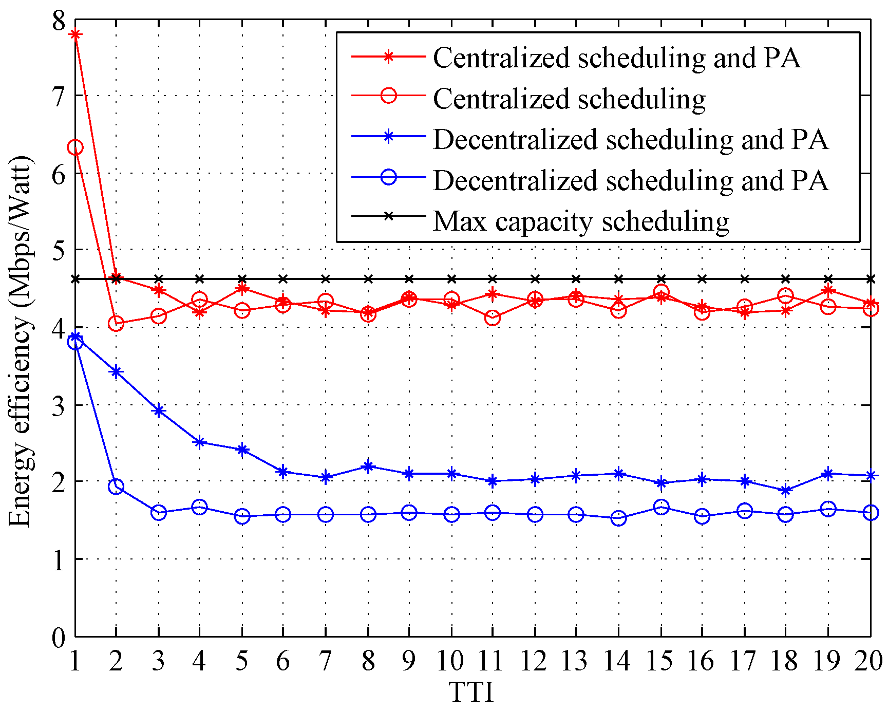More importantly, as shown in Figure 5, the proposed centralized algorithm can also achieve an energy efficiency as good as that of max capacity.

Figure 4. System performances under different resource allocation algorithms (20 Watts, infinite $C_m$, $R_{\text{thres}}=180$ kbps).

Figure 4. System performances under different resource allocation algorithms (20 Watts, infinite $C_m$, $R_{\text{thres}}=180$ kbps).

Figure 5. Energy efficiencies under different resource allocation algorithms (20 Watts, infinite $C_m$, $R_{\text{thres}}=180$ kbps).

Figure 5. Energy efficiencies under different resource allocation algorithms (20 Watts, infinite $C_m$, $R_{\text{thres}}=180$ kbps).

Results in Figure 4 and Figure 5 also compare the performance of the centralized algorithm proposed in Section 4 and that of the decentralized algorithm in Section 5. The results show that both energy efficiency and throughput are decreased when the decentralized algorithm is used.

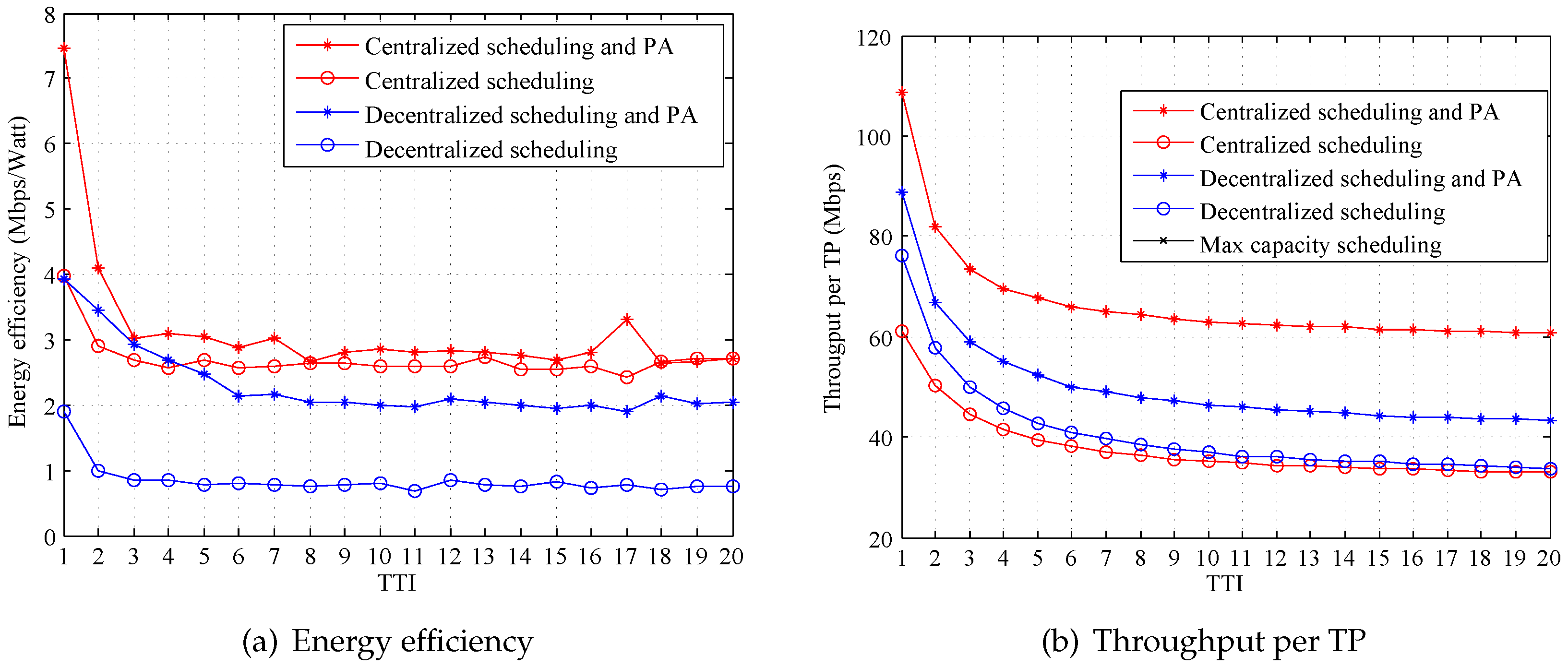
Figure 6 shows the system performances of the proposed algorithms when the transmit power of each TP is 40 Watts. Comparing the results to Figure 4 and Figure 5, it can be seen that the energy efficiency of the centralized algorithm significantly decreases when the transmit power of each TP is up to 40 Watts, while the throughput does not increase. This proves that high-level transmit power is not appropriate in a dense network. Additionally, the results demonstrate that the decentralized algorithm is more robust, since both energy efficiency and throughput are changed a little when different transmit powers are used.

Figure 6. System performance under different strategies (40 Watts, infinite $C_m$, $R_{\text{thres}}=180$ kbps).

Figure 6. System performance under different strategies (40 Watts, infinite $C_m$, $R_{\text{thres}}=180$ kbps).

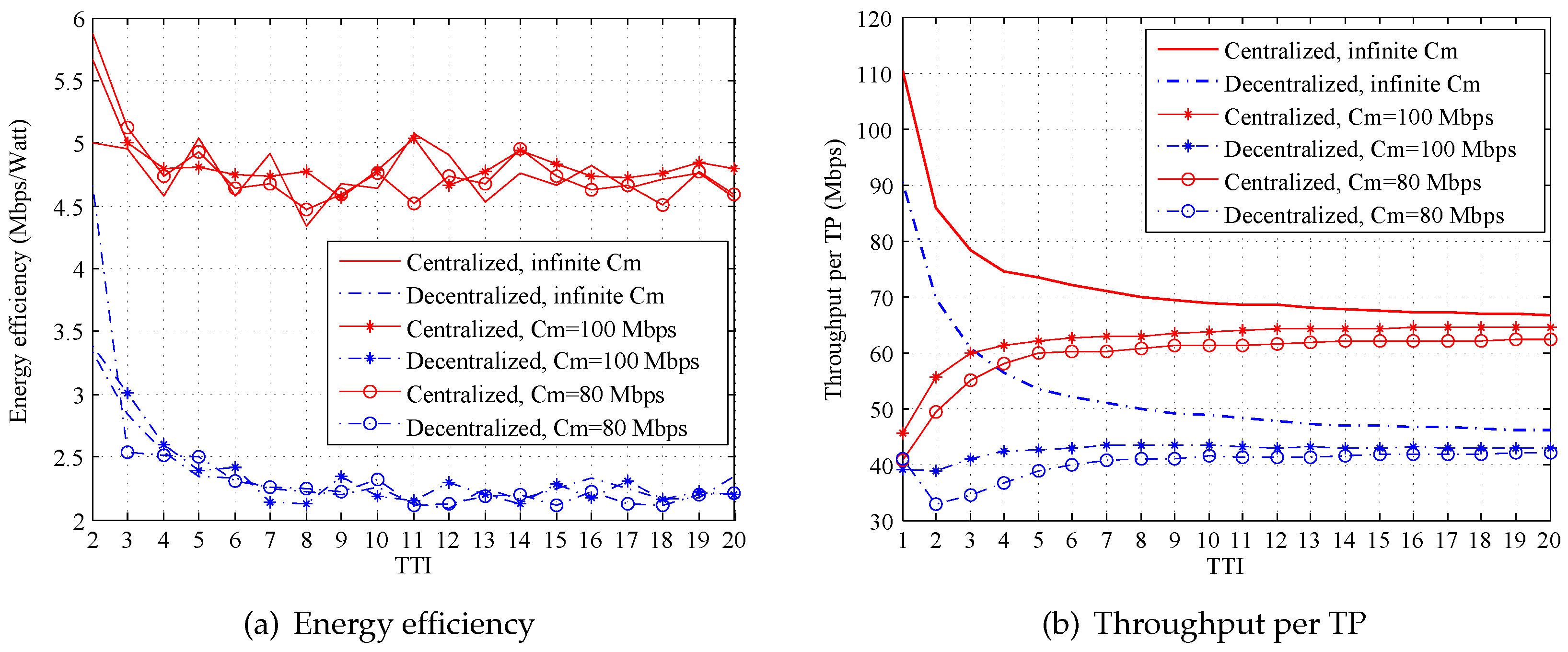
Simulations are also conducted under infinite, 100-Mbps and 80-Mbps backhaul limits, respectively, with a fixed $R_{\text{thres}}$ of 360 kbps, to clearly illustrate the effect on system performance caused by backhaul constraints. Restricted backhaul capacity leads to a low throughput per TP, as shown in Figure 7a, since fewer transmissions are scheduled in this case. However, the tendency is different in terms of energy efficiency. Figure 7b shows that the energy efficiencies of the proposed algorithms under different backhaul limits are almost the same. This is explained by the fact that the power consumed by transmissions is also reduced when backhaul capacity is restricted.

Figure 7. System performance under different backhaul capacity (20 Watts, $R_{\text{thres}}=360$ kbps).

Figure 7. System performance under different backhaul capacity (20 Watts, $R_{\text{thres}}=360$ kbps).

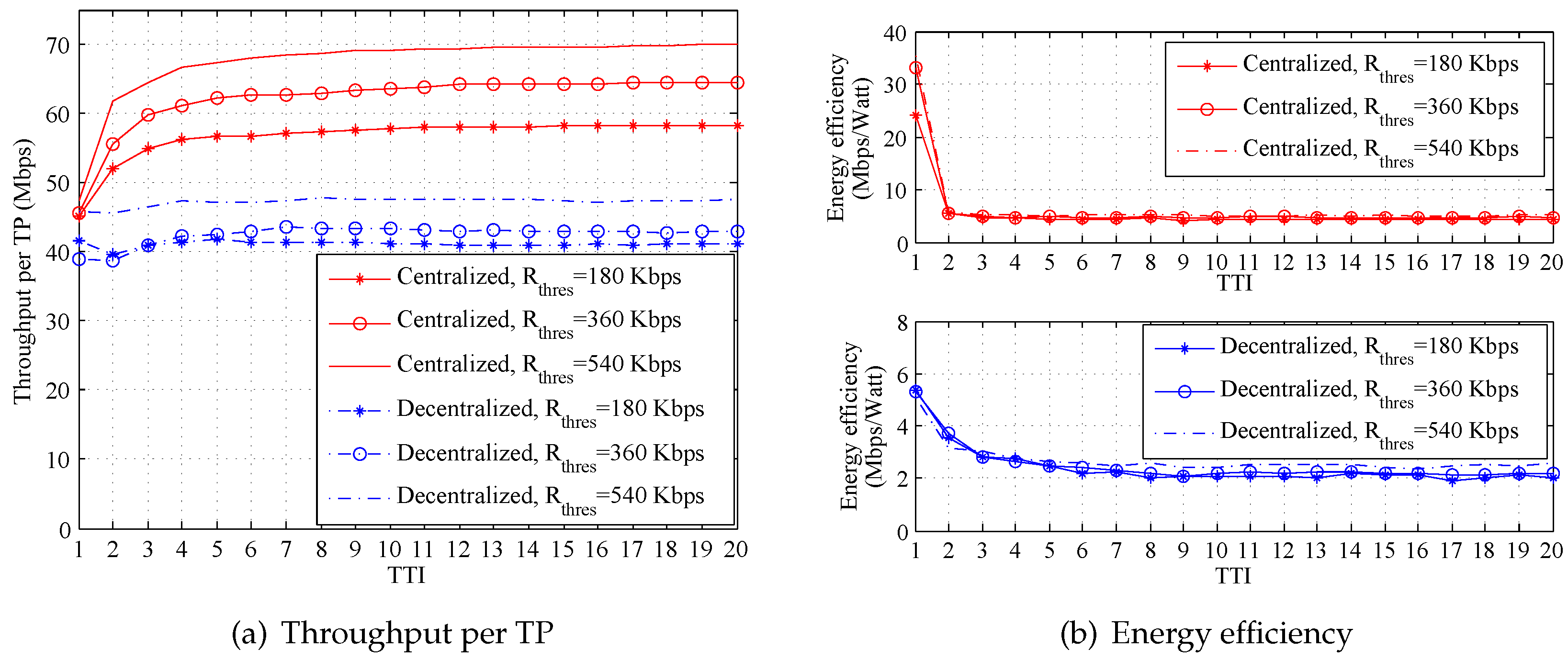
At last, we conduct simulations when $R_{\text{thres}}$ is 180 kbps, 360 kbps and 540 kbps, respectively, with the fixed backhaul capacity of 100 Mbps. This shows that the throughput of our proposals grows as the increase in $R_{\text{thres}}$, as shown in Figure 8a. This is because more resources are assigned to the UEs with better channel conditions, which are possible to achieve for quality transmissions. Figure 8b illustrates that the value of $R_{\text{thres}}$ hardly affects the energy efficiency of the system. Since those transmissions estimated to be inferior to the given $R_{\text{thres}}$ are closed, no (or little) power is wasted. Therefore, that energy efficiency of the system can be maintained at a high level.

Figure 8. System performance under different $R_{\text{thres}}$ (20 Watts, $C_m=100Mbps$).

Figure 8. System performance under different $R_{\text{thres}}$ (20 Watts, $C_m=100Mbps$).

7. Conclusions

In this paper, we have studied a constrained RRM problem aiming at improving energy efficiency in a CoMP-based HetNet. To solve the problem, we first propose a CE-based RB scheduling algorithm under the assumption of equal power allocation. Then, a KKT-based algorithm for power allocation is presented. The proposed algorithms are considered to be used in a centralized way at the first place. Since the centralized strategy for RRM takes a long time delay in large-scale networks, we modified the proposed one in order to adapt to a decentralized system in order to shorten the time delay for processing. Simulation results compare performances of both the centralized and the decentralized and discuss the influence on system performance caused by the considered constraints.

References

1. Damnjanovic, A.; Montojo, J.; Wei, Y.; Ji, T.; Lou, T.; Vajapeyam, M.; Yoo, T.; Song, O.; Malladi, D. A survey on 3GPP heterogeneous networks. Wirel. Commun. 2011, 3, 10–21. [Google Scholar] [CrossRef]
2. Zhang, N.; Cheng, N.; Gamage, A.; Zheng, K.; Mark, J.W.; Shen, X. Cloud Assisted HetNets Toward 5G Wireless Networks. IEEE Commun. 2015, 53, 59–65. [Google Scholar] [CrossRef]
3. Bottai, C.; Cicconetti, C.; Morelli, A.; Resellini, M.; Vitale, C. Energy-efficient user association in extremely dense small cell networks. In Proceedings of the 2014 European Conference on Networks and Communications (EuCNC), Bologna, Italy, 23–26 June 2014; pp. 1–5.
4. Hoydis, J.; Kobayashi, M.; Debbah, M. Green Small-Cell Networks. Veh. Technol. Mag. 2011, 1, 37–43. [Google Scholar] [CrossRef]
5. Rangan, S. Femto-macro cellular interference control with subband scheduling and interference cancelation. In Proceedings of the 2010 IEEE GLOBECOM Workshops (GC Wkshps), Miami, FL, USA, 6–10 December 2010; pp. 695–700.
6. Wang, Y.; Pedersen, K.-I. Performance analysis of enhanced inter-cell interference coordination in LTE-Advanced heterogeneous networks. In Proceedings of the 2012 IEEE 75th Vehicular Technology Conference (VTC Spring), Yokohama, Japan, 6–9 May 2012; pp. 1–5.
7. Peng, M.; Liu, Y.; Wei, D.; Wang, W.; Chen, H. Hierarchical cooperative relay based heterogeneous networks. Wirel. Commun. 2011, 3, 48–56. [Google Scholar] [CrossRef]
8. Irmer, R.; Droste, H.; Marsch, P.; Grieger, M.; Fettweis, G.; Brueck, S.; Mayer, H.-P.; Thiele, L.; Jungnickel, V. Coordinated multipoint: Concepts, performance, and field trial results. IEEE Commun. Mag. 2011, 2, 102–111. [Google Scholar] [CrossRef]
9. LG Electronics. CoMP configurations and UE/eNB behaviors in LTE-Advanced; R1-090213. In Proceedings of the 3GPP TSG RAN WG1 Meeting, Ljubljana, Slovenia, 12–17 January 2009.
10. Tombaz, S.; Vastberg, A.; Zander, J. Energy-and-cost-efficient ultra-high-capacity wireless access. Wirel. Commun. 2011, 5, 18–24. [Google Scholar] [CrossRef]
11. Maattanen, H.; Hamalainen, K.; Venalaiene, J.; Schober, K.; Enescu, M.; Valkama, M. System-level performance of LTE-Advanced with joint transmission and dynamic point selection schemes. EURSIP J. Adv. Signal Process. 2012, 247, 1–18. [Google Scholar]
12. Introduction to Downlink Physical Layer Design. In LTE, The UMTS Long Term Evolution—from Theory to Practice, 2nd ed.; Sesia, S.; Toufik, I.; Baker, M. (Eds.) Wiley: West Sussex, United Kingdom, 2009; pp. 135–137.
13. Yu, W.; Kwon, T.; Shin, C. Multicell coordination via joint scheduling, beamforming and power spectrum adaptation. IEEE Trans. Wirel. Commun. 2013, 7, 1–14. [Google Scholar] [CrossRef]
14. Shen, Z.; Andrews, J.-G.; Evans, B.-L. Adaptive resource allocation in multiuser ofdm systems with proportional rate constraints. IEEE Trans. Wirel. Commun. 2005, 6, 2726–2737. [Google Scholar] [CrossRef]
15. Rubinstein, R.-Y. Optimization of computer simulation models with rare events. Eur. J. Oper. Res. 1997, 1, 89–112. [Google Scholar] [CrossRef]
16. Palomar, D.; Chiang, M. A tutorial on decomposition methods for network utility maximization. IEEE J. Select. Areas Commun. 2006, 8, 1439–1451. [Google Scholar] [CrossRef]
17. Salo, J.; Galdo, G.-D.; Salmi, J.; Kyosti, P.; Milojevic, M.; Laselva, D.; Schneider, C. MATLAB implementation of the 3GPP spatial channel model. Available online: http://read.pudn.com/downloads86/sourcecode/app/331591/scm_11-01-2005.pdf (accessed on 28 January 2016).
18. Shannon, C.E. A mathematical theory of communication. Bell Syst. Tech. J. 1948, 27, 379–423. [Google Scholar] [CrossRef]