
Information Extraction Under Privacy Constraints †

Department of Mathematics and Statistics, Queen’s University, Kingston, Canada
*
Author to whom correspondence should be addressed.
†
Parts of the results in this paper were presented at the 52nd Allerton Conference on Communications, Control and Computing [1] and the 14th Canadian Workshop on Information Theory [2].
Information 2016, 7(1), 15; https://doi.org/10.3390/info7010015
Submission received: 1 November 2015
/
Revised: 24 February 2016
/
Accepted: 3 March 2016
/
Published: 10 March 2016
(This article belongs to the Special Issue Communication Theory)
Abstract
:A privacy-constrained information extraction problem is considered where for a pair of correlated discrete random variables governed by a given joint distribution, an agent observes Y and wants to convey to a potentially public user as much information about Y as possible while limiting the amount of information revealed about X. To this end, the so-called rate-privacy function is investigated to quantify the maximal amount of information (measured in terms of mutual information) that can be extracted from Y under a privacy constraint between X and the extracted information, where privacy is measured using either mutual information or maximal correlation. Properties of the rate-privacy function are analyzed and its information-theoretic and estimation-theoretic interpretations are presented for both the mutual information and maximal correlation privacy measures. It is also shown that the rate-privacy function admits a closed-form expression for a large family of joint distributions of . Finally, the rate-privacy function under the mutual information privacy measure is considered for the case where has a joint probability density function by studying the problem where the extracted information is a uniform quantization of Y corrupted by additive Gaussian noise. The asymptotic behavior of the rate-privacy function is studied as the quantization resolution grows without bound and it is observed that not all of the properties of the rate-privacy function carry over from the discrete to the continuous case.
1. Introduction
With the emergence of user-customized services, there is an increasing desire to balance between the need to share data and the need to protect sensitive and private information. For example, individuals who join a social network are asked to provide information about themselves which might compromise their privacy. However, they agree to do so, to some extent, in order to benefit from the customized services such as recommendations and personalized searches. As another example, a participatory technology for estimating road traffic requires each individual to provide her start and destination points as well as the travel time. However, most participating individuals prefer to provide somewhat distorted or false information to protect their privacy. Furthermore, suppose a software company wants to gather statistical information on how people use its software. Since many users might have used the software to handle some personal or sensitive information -for example, a browser for anonymous web surfing or a financial management software- they may not want to share their data with the company. On the other hand, the company cannot legally collect the raw data either, so it needs to entice its users. In all these situations, a tradeoff in a conflict between utility advantage and privacy breach is required and the question is how to achieve this tradeoff. For example, how can a company collect high-quality aggregate information about users while strongly guaranteeing to its users that it is not storing user-specific information?
To deal with such privacy considerations, Warner [3] proposed the randomized response model in which each individual user randomizes her own data using a local randomizer (i.e., a noisy channel) before sharing the data to an untrusted data collector to be aggregated. As opposed to conditional security, see, e.g., [4,5,6], the randomized response model assumes that the adversary can have unlimited computational power and thus it provides unconditional privacy. This model, in which the control of private data remains in the users’ hands, has been extensively studied since Warner. As a special case of the randomized response model, Duchi et al. [7], inspired by the well-known privacy guarantee called differential privacy introduced by Dwork et al. [8,9,10], introduced locally differential privacy (LDP). Given a random variable , another random variable is said to be the ε-LDP version of X if there exists a channel such that for all measurable and all . The channel Q is then called as the ε-LDP mechanism. Using Jensen’s inequality, it is straightforward to see that any ε-LDP mechanism leaks at most ε bits of private information, i.e., the mutual information between X and Z satisfies .
There have been numerous studies on the tradeoff between privacy and utility for different examples of randomized response models with different choices of utility and privacy measures. For instance, Duchi et al. [7] studied the optimal ε-LDP mechanism which minimizes the risk of estimation of a parameter θ related to . Kairouz et al. [11] studied an optimal ε-LDP mechanism in the sense of mutual information, where an individual would like to release an ε-LDP version Z of X that preserves as much information about X as possible. Calmon et al. [12] proposed a novel privacy measure (which includes maximal correlation and chi-square correlation) between X and Z and studied the optimal privacy mechanism (according to their privacy measure) which minimizes the error probability for any estimator .
In all above examples of randomized response models, given a private source, denoted by X, the mechanism generates Z which can be publicly displayed without breaching the desired privacy level. However, in a more realistic model of privacy, we can assume that for any given private data X, nature generates Y, via a fixed channel . Now we aim to release a public display Z of Y such that the amount of information in Y is preserved as much as possible while Z satisfies a privacy constraint with respect to X. Consider two communicating agents Alice and Bob. Alice collects all her measurements from an observation into a random variable Y and ultimately wants to reveal this information to Bob in order to receive a payoff. However, she is worried about her private data, represented by X, which is correlated with Y. For instance, X might represent her precise location and Y represents measurement of traffic load of a route she has taken. She wants to reveal these measurements to an online road monitoring system to received some utility. However, she does not want to reveal too much information about her exact location. In such situations, the utility is measured with respect to Y and privacy is measured with respect to X. The question raised in this situation then concerns the maximum payoff Alice can get from Bob (by revealing Z to him) without compromising her privacy. Hence, it is of interest to characterize such competing objectives in the form of a quantitative tradeoff. Such a characterization provides a controllable balance between utility and privacy.
This model of privacy first appears in Yamamoto’s work [13] in which the rate-distortion-equivocation function is defined as the tradeoff between a distortion-based utility and privacy. Recently, Sankar et al. [14], using the quantize-and-bin scheme [15], generalized Yamamoto’s model to study privacy in databases from an information-theoretic point of view. Calmon and Fawaz [16] and Monedero et al. [17] also independently used distortion and mutual information for utility and privacy, respectively, to define a privacy-distortion function which resembles the classical rate-distortion function. More recently, Makhdoumi et al. [18] proposed to use mutual information for both utility and privacy measures and defined the privacy funnel as the corresponding privacy-utility tradeoff, given by
where denotes that and Z form a Markov chain in this order. Leveraging well-known algorithms for the information bottleneck problem [19], they provided a locally optimal greedy algorithm to evaluate . Asoodeh et al. [1], independently, defined the rate-privacy function, , as the maximum achievable such that Z satisfies , which is a dual representation of the privacy funnel (1), and showed that for discrete X and Y, if and only if X is weakly independent of Y (cf, Definition 9). Recently, Calmon et al. [20] proved an equivalent result for using a different approach. They also obtained lower and upper bounds for which can be easily translated to bounds for (cf. Lemma 1). In this paper, we develop further properties of and also determine necessary and sufficient conditions on , satisfying some symmetry conditions, for to achieve its upper and lower bounds.
The problem treated in this paper can also be contrasted with the better-studied concept of secrecy following the pioneering work of Wyner [21]. While in secrecy problems the aim is to keep information secret only from wiretappers, in privacy problems the aim is to keep the private information (not necessarily all the information) secret from everyone including the intended receiver.
1.1. Our Model and Main Contributions
Using mutual information as measure of both utility and privacy, we formulate the corresponding privacy-utility tradeoff for discrete random variables X and Y via the rate-privacy function, , in which the mutual information between Y and displayed data (i.e., the mechanism’s output), Z, is maximized over all channels such that the mutual information between Z and X is no larger than a given ε. We also formulate a similar rate-privacy function where the privacy is measured in terms of the squared maximal correlation, , between, X and Z. In studying and , any channel that satisfies and , preserves the desired level of privacy and is hence called a privacy filter. Interpreting as the number of bits that a privacy filter can reveal about Y without compromising privacy, we present the rate-privacy function as a formulation of the problem of maximal privacy-constrained information extraction from Y.
We remark that using maximal correlation as a privacy measure is by no means new as it appears in other works, see, e.g., [22,23] and [12] for different utility functions. We do not put any likelihood constraints on the privacy filters as opposed to the definition of LDP. In fact, the optimal privacy filters that we obtain in this work induce channels that do not satisfy the LDP property.
The quantity is related to a notion of the reverse strong data processing inequality as follows. Given a joint distribution , the strong data processing coefficient was introduced in [24,25], as the smallest such that for all satisfying the Markov condition . In the rate-privacy function, we instead seek an upper bound on the maximum achievable rate at which Y can display information, , while meeting the privacy constraint . The connection between the rate-privacy function and the strong data processing inequality is further studied in [20] to mirror all the results of [25] in the context of privacy.
The contributions of this work are as follows:
- We study lower and upper bounds of . The lower bound, in particular, establishes a multiplicative bound on for any optimal privacy filter. Specifically, we show that for a given and there exists a channel such that andwhere is a constant depending on the joint distribution . We then give conditions on such that the upper and lower bounds are tight. For example, we show that the lower bound is achieved when Y is binary and the channel from Y to X is symmetric. We show that this corresponds to the fact that both and induce distributions and which are equidistant from in the sense of Kullback-Leibler divergence. We then show that the upper bound is achieved when Y is an erased version of X, or equivalently, is an erasure channel.
- We propose an information-theoretic setting in which appears as a natural upper-bound for the achievable rate in the so-called "dependence dilution" coding problem. Specifically, we examine the joint-encoder version of an amplification-masking tradeoff, a setting recently introduced by Courtade [26] and we show that the dual of upper bounds the masking rate. We also present an estimation-theoretic motivation for the privacy measure . In fact, by imposing , we require that an adversary who observes Z cannot efficiently estimate , for any function f. This is reminiscent of semantic security [27] in the cryptography community. An encryption mechanism is said to be semantically secure if the adversary’s advantage for correctly guessing any function of the privata data given an observation of the mechanism’s output (i.e., the ciphertext) is required to be negligible. This, in fact, justifies the use of maximal correlation as a measure of privacy. The use of mutual information as privacy measure can also be justified using Fano’s inequality. Note that can be shown to imply that and hence the probability of adversary correctly guessing X is lower-bounded.
- We also study the rate of increase of at and show that this rate can characterize the behavior of for any provided that . This again has connections with the results of [25]. Lettingone can easily show that and hence the rate of increase of at characterizes the strong data processing coefficient. Note that here we have .
- Finally, we generalize the rate-privacy function to the continuous case where X and Y are both continuous and show that some of the properties of in the discrete case do not carry over to the continuous case. In particular, we assume that the privacy filter belongs to a family of additive noise channels followed by an M-level uniform scalar quantizer and give asymptotic bounds as for the rate-privacy function.
1.2. Organization
The rest of the paper is organized as follows. In Section 2, we define and study the rate-privacy function for discrete random variables for two different privacy measures, which, respectively, lead to the information-theoretic and estimation-theoretic interpretations of the rate-privacy function. In Section 3, we provide such interpretations for the rate-privacy function in terms of quantities from information and estimation theory. Having obtained lower and upper bounds of the rate-privacy function, in Section 4 we determine the conditions on such that these bounds are tight. The rate-privacy function is then generalized and studied in Section 5 for continuous random variables.
2. Utility-Privacy Measures: Definitions and Properties
Consider two random variables X and Y, defined over finite alphabets and , respectively, with a fixed joint distribution . Let X represent the private data and let Y be the observable data, correlated with X and generated by the channel predefined by nature, which we call the observation channel. Suppose there exists a channel such that Z, the displayed data made available to public users, has limited dependence with X. Such a channel is called the privacy filter. This setup is shown in Figure 1. The objective is then to find a privacy filter which gives rise to the highest dependence between Y and Z. To make this goal precise, one needs to specify a measure for both utility (dependence between Y and Z) and also privacy (dependence between X and Z).
2.1. Mutual Information as Privacy Measure
Adopting mutual information as a measure of both privacy and utility, we are interested in characterizing the following quantity, which we call the rate-privacy function (since mutual information is adopted for utility, the privacy-utility tradeoff characterizes the optimal rate for a given privacy level, where rate indicates the precision of the displayed data Z with respect to the observable data Y for a privacy filter, which suggests the name),
where has fixed distribution and
(here means that and Z form a Markov chain in this order). Equivalently, we call the privacy-constrained information extraction function, as Z can be thought of as the extracted information from Y under privacy constraint .
Note that since is a convex function of and furthermore the constraint set is convex, [28, Theorem 32.2] implies that we can restrict in (3) to whenever . Note also that since for finite and , is a continuous map, therefore is compact and the supremum in (3) is indeed a maximum. In this case, using the Support Lemma [29], one can readily show that it suffices that the random variable Z is supported on an alphabet with cardinality . Note further that by the Markov condition , we can always restrict to only , because and hence for the privacy constraint is removed and thus by setting , we obtain .
As mentioned earlier, a dual representation of , the so called privacy funnel, is introduced in [18,20], defined in (1), as the least information leakage about X such that the communication rate is greater than a positive constant; for some . Note that if then .
Given and a joint distribution , we have and hence is non-decreasing, i.e., . Using a similar technique as in [30, Lemma 1], Calmon et al. [20] showed that the mapping is non-decreasing for . This, in fact, implies that is non-increasing for . This observation leads to a lower bound for the rate privacy function as described in the following lemma.
Lemma 1
([20]). For a given joint distribution P defined over , the mapping is non-increasing on and lies between two straight lines as follows:
for .
Using a simple calculation, the lower bound in (4) can be shown to be achieved by the privacy filter depicted in Figure 2 with the erasure probability
In light of Lemma 1, the possible range of the map is as depicted in Figure 3.
We next show that is concave and continuous.
Lemma 2.
For any given pair of random variables over , the mapping is concave for .
Proof.
It suffices to show that for any , we have
which, in turn, is equivalent to
Let and be two optimal privacy filters in and with disjoint output alphabets and , respectively.
We introduce an auxiliary binary random variable , independent of , where and define the following random privacy filter : We pick if and if , and let be the output of this random channel which takes values in . Note that . Then we have
which implies that . On the other hand, we have
which, according to (7), completes the proof. ☐
Remark 1.
By the concavity of , we can show that is a strictly increasing function of . To see this, assume there exists such that . Since is concave, then it follows that for all , and since for , , implying that for any , we must have which contradicts the upper bound shown in (4).
Corollary 3.
For any given pair of random variables over , the mapping is continuous for .
Proof.
Concavity directly implies that the mapping is continuous on (see for example [31, Theorem 3.2]). Continuity at zero follows from the continuity of mutual information. ☐
Remark 2.
Using the concavity of the map , we can provide an alternative proof for the lower bound in (4). Note that point is always on the curve , and hence by concavity, the straight line is always below the lower convex envelop of , i.e., the chord connecting to , and hence . In fact, this chord yields a better lower bound for on as
which reduces to the lower bound in (4) only if .
2.2. Maximal Correlation as Privacy Measure
By adopting the mutual information as the privacy measure between the private and the displayed data, we make sure that only limited bits of private information is revealed during the process of transferring Y. In order to have an estimation theoretic guarantee of privacy, we propose alternatively to measure privacy using a measure of correlation, the so-called maximal correlation.
Given the collection of all pairs of random variables where and are general alphabets, a mapping defines a measure of correlation [32] if if and only if U and V are independent (in short, ) and attains its maximum value if or almost surely for some measurable real-valued functions f and g. There are many different examples of measures of correlation including the Hirschfeld-Gebelein-Rényi maximal correlation [32,33,34], the information measure [35], mutual information and f-divergence [36].
Definition 4
([34]). Given random variables X and Y, the maximal correlation is defined as follows (recall that the correlation coefficient between U and V, is defined as , where and are the covariance between U and V, the standard deviations of U and V, respectively):
where is the collection of pairs of real-valued random variables and such that and . If is empty (which happens precisely when at least one of X and Y is constant almost surely) then one defines to be 0. Rényi [34] derived an equivalent characterization of maximal correlation as follows:
Measuring privacy in terms of maximal correlation, we propose
as the corresponding rate-privacy tradeoff, where
Again, we equivalently call as the privacy-constrained information extraction function, where here the privacy is guaranteed by .
Setting corresponds to the case where X and Z are required to be statistically independent, i.e., absolutely no information leakage about the private source X is allowed. This is called perfect privacy. Since the independence of X and Z is equivalent to , we have . However, for , both and might happen in general. For general , it directly follows using [23, Proposition 1] that
where and
Similar to , we see that for , and hence is non-decreasing. The following lemma is a counterpart of Lemma 1 for .
Lemma 5.
For a given joint distribution defined over , is non-increasing on .
Proof.
Like Lemma 1, the proof is similar to the proof of [30, Lemma 1]. We, however, give a brief proof for the sake of completeness.
For a given channel and , we can define a new channel with an additional symbol e as follows
It is easy to check that and also ; see [37, Page 8], which implies that where . Now suppose that achieves , that is, and . We can then write
Therefore, for we have . ☐
Similar to the lower bound for obtained from Lemma 1, we can obtain a lower bound for using Lemma 5. Before we get to the lower bound, we need a data processing lemma for maximal correlation. The following lemma proves a version of strong data processing inequality for maximal correlation from which the typical data processing inequality follows, namely, for and Z satisfying .
Lemma 6.
For random variables X and Y with a joint distribution , we have
Proof.
For arbitrary zero-mean and unit variance measurable functions and and , we have
where the inequality follows from the Cauchy-Schwartz inequality and (9). Thus we obtain .
This bound is tight for the special case of , where is the backward channel associated with . In the following, we shall show that .
To this end, first note that the above implies that . Since , it follows that and hence the above implies that . One the other hand, we have
which together with (9) implies that
Thus, which completes the proof. ☐
Now a lower bound of can be readily obtained.
Corollary 7.
For a given joint distribution defined over , we have for any
Proof.
By Lemma 6, we know that for any Markov chain , we have and hence for , the privacy constraint is not restrictive and hence by setting . For , Lemma 5 implies that
from which the result follows. ☐
A loose upper bound of can be obtained using an argument similar to the one used for . For the Markov chain , we have
where and comes from [23, Proposition 1]. We can, therefore, conclude from (11) and Corollary 7 that
Similar to Lemma 2, the following lemma shows that the is a concave function of ε.
Lemma 8.
For any given pair of random variables with distribution P over , the mapping is concave for .
Proof.
The proof is similar to that of Lemma 2 except that here for two optimal filters and in and , respectively, and the random channel with output alphabet constructed using a coin flip with probability γ, we need to show that , where . To show this, consider such that and and let U be a binary random variable as in the proof of Lemma 2. We then have
where comes from the fact that U is independent of X. We can then conclude from (13) and the alternative characterization of maximal correlation (9) that
from which we can conclude that . ☐
2.3. Non-Trivial Filters For Perfect Privacy
As it becomes clear later, requiring that is a useful assumption for the analysis of . Thus, it is interesting to find a necessary and sufficient condition on the joint distribution which results in .
Definition 9
([38]). The random variable X is said to be weakly independent of Y if the rows of the transition matrix , i.e., the set of vectors , are linearly dependent.
The following lemma provides a necessary and sufficient condition for .
Lemma 10.
For a given with a given joint distribution , (and equivalently ) if and only if X is weakly independent of Y.
Proof.
⇒ direction:
Assuming that implies that there exists a random variable Z over an alphabet such that the Markov condition is satisfied and while . Hence, for any and in , we must have for all , which implies that
and hence
Since Y is not independent of Z, there exist and such that and hence the above shows that the set of vectors , is linearly dependent.
⇐ direction:
Berger and Yeung [38, Appendix II], in a completely different context, showed that if X being weakly independent of Y, one can always construct a binary random variable Z correlated with Y which satisfies and , and hence . ☐
Remark 3.
Lemma 10 first appeared in [1]. However, Calmon et al. [20] studied (1), the dual version of , and showed an equivalent result for . In fact, they showed that for a given , one can always generate Z such that , and , or equivalently , if and only if the smallest singular value of the conditional expectation operator is zero. This condition can, in fact, be shown to be equivalent to the condition in Lemma 10.
Remark 4.
It is clear that, according to Definition 9, X is weakly independent of Y if . Hence, Lemma 10 implies that if Y has strictly larger alphabet than X.
In light of the above remark, in the most common case of , one might have , which corresponds to the most conservative scenario as no privacy leakage implies no broadcasting of observable data. In such cases, the rate of increase of at , that is , which corresponds to the initial efficiency of privacy-constrained information extraction, proves to be very important in characterizing the behavior of for all . This is because, for example, by concavity of , the slope of is maximized at and so
and hence for all which, together with (4), implies that if . In the sequel, we always assume that X is not weakly independent of Y, or equivalently . For example, in light of Lemma 10 and Remark 4, we can assume that .
It is easy to show that, X is weakly independent of binary Y if and only if X and Y are independent (see, e.g., [38, Remark 2]). The following corollary, therefore, immediately follows from Lemma 10.
Corollary 11.
Let Y be a non-degenerate binary random variable correlated with X. Then .
3. Operational Interpretations of the Rate-Privacy Function
In this section, we provide a scenario in which appears as a boundary point of an achievable rate region and thus giving an information-theoretic operational interpretation for . We then proceed to present an estimation-theoretic motivation for .
3.1. Dependence Dilution
Inspired by the problems of information amplification [39] and state masking [40], Courtade [26] proposed the information-masking tradeoff problem as follows. The tuple is said to be achievable if for two given separated sources and and any there exist mappings and such that and . In other words, is achievable if there exist indices K and J of rates and given and , respectively, such that the receiver in possession of can recover at most bits about and at least about . The closure of the set of all achievable tuple is characterized in [26]. Here, we look at a similar problem but for a joint encoder. In fact, we want to examine the achievable rate of an encoder observing both and which masks and amplifies at the same time, by rates and , respectively.
We define a dependence dilution code by an encoder
and a list decoder
where denotes the power set of . A dependence dilution triple is said to be achievable if, for any , there exists a dependence dilution code that for sufficiently large n satisfies the utility constraint:
having a fixed list size
where is the encoder’s output, and satisfies the privacy constraint:
Intuitively speaking, upon receiving J, the decoder is required to construct list of fixed size which contains likely candidates of the actual sequence . Without any observation, the decoder can only construct a list of size which contains with probability close to one. However, after J is observed and the list is formed, the decoder’s list size can be reduced to and thus reducing the uncertainty about by . This observation led Kim et al. [39] to show that the utility constraint (14) is equivalent to the amplification requirement
which lower bounds the amount of information J carries about . The following lemma gives an outer bound for the achievable dependence dilution region.
Theorem 12.
Any achievable dependence dilution triple satisfies
for some auxiliary random variable with a finite alphabet and jointly distributed with X and Y.
Before we prove this theorem, we need two preliminary lemmas. The first lemma is an extension of Fano’s inequality for list decoders and the second one makes use of a single-letterization technique to express in a single-letter form in the sense of Csiszár and Körner [29].
Lemma 13
This lemma, applied to J and in place of U and V, respectively, implies that for any list decoder with the property (14), we have
where and hence as .
Lemma 14.
Let be n i.i.d. copies of a pair of random variables . Then for a random variable J jointly distributed with , we have
where .
Proof.
Using the chain rule for the mutual information, we can express as follows
Similarly, we can expand as
Subtracting (20) from (19), we get
where follows from the Csiszár sum identity [42]. ☐
Proof of Theorem 12.
The rate R can be bounded as
where follows from Fano’s inequality (18) with as and is due to (15). We can also upper bound as
where follows from (15), follows from (18), and in the last equality the auxiliary random variable is introduced.
We shall now lower bound :
where follows from Lemma 14 and is due to Fano’s inequality and (15) (or equivalently from (17)).
Combining (22), (23) and (24), we can write
where and Q is a random variable distributed uniformly over which is independent of and hence . The results follow by denoting and noting that and have the same distributions as Y and X, respectively. ☐
If the encoder does not have direct access to the private source , then we can define the encoder mapping as . The following corollary is an immediate consequence of Theorem 12.
Corollary 15.
If the encoder does not see the private source, then for all achievable dependence dilution triple , we have
for some joint distribution where the auxiliary random variable satisfies .
Remark 5.
If source Y is required to be amplified (according to (17)) at maximum rate, that is, for an auxiliary random variable U which satisfies , then by Corollary 15, the best privacy performance one can expect from the dependence dilution setting is
which is equal to the dual of evaluated at , , as defined in (1).
The dependence dilution problem is closely related to the discriminatory lossy source coding problem studied in [15]. In this problem, an encoder f observes and wants to describe this source to a decoder, g, such that g recovers within distortion level D and . If the distortion level is Hamming measure, then the distortion constraint and the amplification constraint are closely related via Fano’s inequality. Moreover, dependence dilution problem reduces to a secure lossless (list decoder of fixed size 1) source coding problem by setting , which is recently studied in [43].
3.2. MMSE Estimation of Functions of Private Information
In this section, we provide a justification for the privacy guarantee . To this end, we recall the definition of the minimum mean squared error estimation.
Definition 16.
Given random variables U and V, is defined as the minimum error of an estimate, , of U based on V, measured in the mean-square sense, that is
where denotes the conditional variance of U given V.
It is easy to see that if and only if for some measurable function f and if and only if . Hence, unlike for the case of maximal correlation, a small value of implies a strong dependence between U and V. Hence, although it is not a "proper" measure of correlation, in a certain sense it measures how well one random variable can be predicted from another one.
Given a non-degenerate measurable function , consider the following constraint on
This guarantees that no adversary knowing Z can efficiently estimate . First consider the case where f is an identity function, i.e., . In this case, a direct calculation shows that
where follows from (26) and is due to the definition of maximal correlation. Having imposed , we, can therefore conclude that the MMSE of estimating X given Z satisfies
which shows that implies (27) for . However, in the following we show that the constraint is, indeed, equivalent to (27) for any non-degenerate measurable .
Definition 17
([44]). A joint distribution satisfies a Poincaré inequality with constant if for all
and the Poincaré constant for is defined as
The privacy constraint (27) can then be viewed as
Theorem 18
In light of Theorem 18 and (29), the privacy constraint (27) is equivalent to , that is,
for any non-degenerate measurable functions .
Hence, characterizes the maximum information extraction from Y such that no (non-trivial) function of X can be efficiently estimated, in terms of MMSE (27), given the extracted information.
4. Observation Channels for Minimal and Maximal
In this section, we characterize the observation channels which achieve the lower or upper bounds on the rate-privacy function in (4). We first derive general conditions for achieving the lower bound and then present a large family of observation channels which achieve the lower bound. We also give a family of which attain the upper bound on .
4.1. Conditions for Minimal
Assuming that , we seek a set of conditions on such that is linear in ε, or equivalently, . In order to do this, we shall examine the slope of at zero. Recall that by concavity of , it is clear that . We strengthen this bound in the following lemmas. For this, we need to recall the notion of Kullback-Leibler divergence. Given two probability distribution P and Q supported over a finite alphabet ,
Lemma 19.
For a given joint distribution , if , then for any
Proof.
The proof is given in Appendix A. ☐
Remark 6.
Note that if for a given joint distribution , there exists such that , it implies that . Consider the binary random variable constructed according to the distribution and for . We can now claim that Z is independent of X, because and
Clearly, Z and Y are not independent, and hence . This implies that the right-hand side of inequality in Lemma 19 can not be infinity.
In order to prove the main result, we need the following simple lemma.
Lemma 20.
For any joint distribution , we have
where equality holds if and only if there exists a constant such that for all .
Proof.
It is clear that
where the inequality follows from the fact that for any three sequences of positive numbers , and we have where equality occurs if and only if for all . ☐
Now we are ready to state the main result of this subsection.
Theorem 21.
For a given with joint distribution , if and is linear for , then for any
Proof.
Note that the fact that and is linear in ε is equivalent to . It is, therefore, immediate from Lemmas 19 and 20 that we have
where follows from the fact that and and are due to Lemmas 20 and 19, respectively. The inequality in (31) shows that
According to Lemma 20, (32) implies that the ratio of does not depend on and hence the result follows. ☐
This theorem implies that if there exists and such that results in two different values, then cannot achieve the lower bound in (4), or equivalently
This, therefore, gives a necessary condition for the lower bound to be achievable. The following corollary simplifies this necessary condition.
Corollary 22.
For a given joint distribution , if and is linear, then the following are equivalent:
- (i)
- Y is uniformly distributed,
- (ii)
- is constant for all .
Proof.
:
From Theorem 21, we have for all
Letting for any , we have and hence , which together with (33) implies that for all and hence Y is uniformly distributed.
:
When Y is uniformly distributed, we have from (33) that which implies that is constant for all . ☐
Example 1.
Suppose is a binary symmetric channel (BSC) with crossover probability and . In this case, is also a BSC with input distribution . Note that Corollary 11 implies that . We will show that is linear as a function of for a larger family of symmetric channels (including BSC) in Corollary 24. Hence, the BSC with uniform input nicely illustrates Corollary 22, because for .
Example 2.
Now suppose is a binary asymmetric channel such that , for some and input distribution , . It is easy to see that if then does not depend on y and hence we can conclude from Corollary 22 (noticing that ) that in this case for any , is not linear and hence for
In Theorem 21, we showed that when achieves its lower bound, illustrated in (4), the slope of the mapping at zero is equal to for any . We will show in the next section that the reverse direction is also true at least for a large family of binary-input symmetric output channels, for instance when is a BSC, and thus showing that in this case,
4.2. Special Observation Channels
In this section, we apply the results of last section to different joint distributions . In the first family of channels from X to Y, we look at the case where Y is binary and the reverse channel has symmetry in a particular sense, which will be specified later. One particular case of this family of channels is when is a BSC. As a family of observation channels which achieves the upper bound of , stated in (4), we look at the class of erasure channels from , i.e., Y is an erasure version of X.
4.2.1. Observation Channels With Symmetric Reverse
The first example of that we consider for binary Y is the so-called Binary Input Symmetric Output (BISO) , see for example [45,46]. Suppose and , and for any we have . This clearly implies that . We notice that with this definition of symmetry, we can always assume that the output alphabet has even number of elements because we can split into two outputs, and , with and . The new channel is clearly essentially equivalent to the original one, see [46] for more details. This family of channels can also be characterized using the definition of quasi-symmetric channels [47, Definition 4.17]. A channel is BISO if (after making even) the transition matrix can be partitioned along its columns into binary-input binary-output sub-arrays in which rows are permutations of each other and the column sums are equal. It is clear that binary symmetric channels and binary erasure channels are both BISO. The following lemma gives an upper bound for when belongs to such a family of channels.
Lemma 23.
If the channel is BISO, then for ,
where denotes the capacity of .
Proof.
The lower bound has already appeared in (4). To prove the upper bound note that by Markovity , we have for any and
Now suppose and similarly . Then (34) allows us to write for
where is the inverse of binary entropy function, and for ,
Letting and denote the right-hand sides of (35) and (36), respectively, we can, hence, write
where denotes the entropy of X when Y is uniformly distributed. Here, is due to (35) and (36), follows form convexity of for all [48] and Jensen’s inequality. In , we used the symmetry of channel to show that . Hence, we obtain
where the equality follows from the fact that for BISO channel (and in general for any quasi-symmetric channel) the uniform input distribution is the capacity-achieving distribution [47, Lemma 4.18]. Since is attained when , the conclusion immediately follows. ☐
This lemma then shows that the larger the gap between and is for , the more deviates from its lower bound. When , then and and hence Lemma 23 implies that
and hence we have proved the following corollary.
Corollary 24.
If the channel is BISO and , then for any
This corollary now enables us to prove the reverse direction of Theorem 21 for the family of BISO channels.
Theorem 25.
If is a BISO channel, then the following statements are equivalent:
- (i)
- for .
- (ii)
- The initial efficiency of privacy-constrained information extraction is
Proof.
(i)⇒ (ii).
This follows from Theorem 21.
(ii)⇒ (i).
Let for , and, as before, , so that is determined by a matrix. We then have
and
The hypothesis implies that (37) is equal to (38), that is,
It is shown in Appendix B that (39) holds if and only if . Now we can invoke Corollary 24 to conclude that . ☐
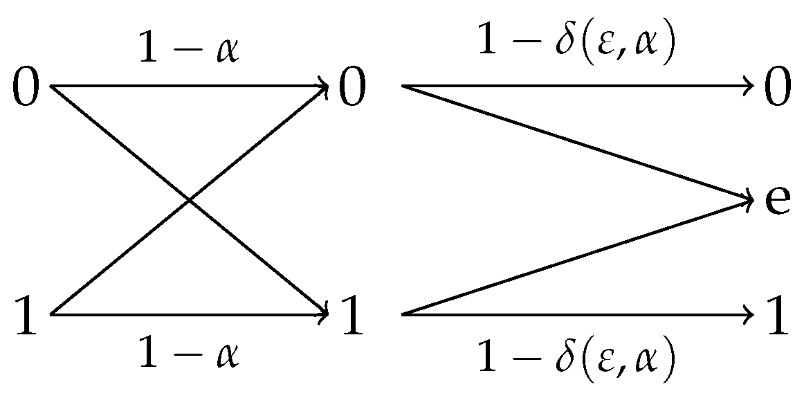
This theorem shows that for any BISO channel with uniform input, the optimal privacy filter is an erasure channel depicted in Figure 2. Note that if is a BSC with uniform input , then is also a BSC with uniform input . The following corollary specializes Corollary 24 for this case.
Corollary 26.
For the joint distribution , the binary erasure channel with erasure probability (shown in Figure 4)
for , is the optimal privacy filter in (3). In other words, for
Moreover, for a given , is the only distribution for which is linear. That is, for , , we have
Proof.
As mentioned earlier, since and is , it follows that is also a BSC with uniform input and hence from Corollary 24, we have . As in this case achieves the lower bound given in Lemma 1, we conclude from Figure 2 that BEC(), where , is an optimal privacy filter. The fact that is the only input distribution for which is linear follows from the proof of Theorem 25. In particular, we saw that a necessary and sufficient condition for being linear is that the ratio is constant for all . As shown before, this is equivalent to . For the binary symmetric channel, this is equivalent to . ☐
The optimal privacy filter for BSC(α) and uniform X is shown in Figure 4. In fact, this corollary immediately implies that the general lower-bound given in (4) is tight for the binary symmetric channel with uniform X.
4.2.2. Erasure Observation Channel
Combining (8) and Lemma 1, we have for
In the following we show that the above upper and lower bound coincide when is an erasure channel, i.e., and for all and .
Lemma 27.
For any given , if is an erasure channel (as defined above), then
for any .
Proof.
It suffices to show that if is an erasure channel, then . This follows, since if , then the lower bound in (41) becomes and thus .
Let and where e denotes the erasure symbol. Consider the following privacy filter to generate :
For any , we have
which implies and thus . On the other hand, , and therefore we have
It then follows from Lemma 1 that , which completes the proof. ☐
Example 3.
In light of this lemma, we can conclude that if , then the optimal privacy filter is a combination of an identity channel and a BSC(), as shown in Figure 5, where is the unique solution of
where , and . Note that it is easy to check that . Therefore, in order for this channel to be a valid privacy filter, the crossover probability, , must be chosen such that . We note that for fixed and , the map is monotonically decreasing on ranging over and since , the solution of the above equation is unique.
Combining Lemmas 1 and 27 with Corollary 26, we can show the following extremal property of the BEC and BSC channels, which is similar to other existing extremal properties of the BEC and the BSC, see, e.g., [46] and [45]. For , we have for any channel ,
where is the rate-privacy function corresponding to and . Similarly, if , we have for any channel with ,
where is the rate-privacy function corresponding to and .
5. Rate-Privacy Function for Continuous Random Variables
In this section we extend the rate-privacy function to the continuous case. Specifically, we assume that the private and observable data are continuous random variables and that the filter is composed of two stages: first Gaussian noise is added and then the resulting random variable is quantized using an M-bit accuracy uniform scalar quantizer (for some positive integer ). These filters are of practical interest as they can be easily implemented. This section is divided in two subsections, in the first we discuss general properties of the rate-privacy function and in the second we study the Gaussian case in more detail. Some observations on for continuous X and Y are also given.
5.1. General Properties of the Rate-Privacy Function
Throughout this section we assume that the random vector is absolutely continuous with respect to the Lebesgue measure on . Additionally, we assume that its joint density satisfies the following.
- (a)
- There exist constants , and bounded function such thatand also for
- (b)
- and are both finite,
- (c)
- the differential entropy of satisfies ,
- (d)
- , where denotes the largest integer ℓ such that .
Note that assumptions (b) and (c) together imply that , and are finite, i.e., the maps and are integrable. We also assume that X and Y are not independent, since otherwise the problem to characterize becomes trivial by assuming that the displayed data Z can equal the observable data Y.
We are interested in filters of the form where , is a standard normal random variable which is independent of X and Y, and for any positive integer M, denotes the M-bit accuracy uniform scalar quantizer, i.e., for all
Let and . We define, for any ,
and similarly
The next theorem shows that the previous definitions are closely related.
Theorem 28.
Let be fixed. Then .
Proof.
See Appendix C. ☐
In the limit of large M, approximates . This becomes relevant when is easier to compute than , as demonstrated in the following subsection. The following theorem summarizes some general properties of .
Theorem 29.
The function is non-negative, strictly-increasing, and satisfies
Proof.
See Appendix C. ☐
As opposed to the discrete case, in the continuous case is no longer bounded. In the following section we show that can be convex, in contrast to the discrete case where it is always concave.
We can also define and for continuous X and Y, similar to (43) and (44), but where the privacy constraints are replaced by and , respectively. It is clear to see from Theorem 29 that and . However, although we showed that is indeed the asymptotic approximation of for M large enough, it is not clear that the same statement holds for and .
5.2. Gaussian Information
The rate-privacy function for Gaussian Y has an interesting interpretation from an estimation theoretic point of view. Given the private and observable data , suppose an agent is required to estimateY based on the output of the privacy filter. We wish to know the effect of imposing a privacy constraint on the estimation performance.
The following lemma shows that bounds the best performance of the predictability of Y given the output of the privacy filter. The proof provided for this lemma does not use the Gaussianity of the noise process, so it holds for any noise process.
Lemma 30.
For any given private data X and Gaussian observable data Y, we have for any
Proof.
It is a well-known fact from rate-distortion theory that for a Gaussian Y and its reconstruction
and hence by setting , where is an output of a privacy filter, and noting that , we obtain
from which the result follows immediately. ☐
According to Lemma 30, the quantity is a parameter that bounds the difficulty of estimating Gaussian Y when observing an additive perturbation Z with privacy constraint . Note that , and therefore, provided that the privacy threshold is not trivial (i.e, ), the mean squared error of estimating Y given the privacy filter output is bounded away from zero, however the bound decays exponentially at rate of .
To finish this section, assume that X and Y are jointly Gaussian with correlation coefficient ρ. The value of can be easily obtained in closed form as demonstrated in the following theorem.
Theorem 31.
Let be jointly Gaussian random variables with correlation coefficient ρ. For any we have
Proof.
One can always write where and is a Gaussian random variable with mean 0 and variance which is independent of . On the other hand, we have where N is the standard Gaussian random variable independent of and hence . In order for this additive channel to be a privacy filter, it must satisfy
which implies
and hence
Since is strictly decreasing (cf., Appendix C), we obtain
According to (46), we conclude that the optimal privacy filter for jointly Gaussian is an additive Gaussian channel with signal to noise ratio , which shows that if perfect privacy is required, then the displayed data is independent of the observable data Y, i.e., .
Remark 7.
We could assume that the privacy filter adds non-Gaussian noise to the observable data and define the rate-privacy function accordingly. To this end, we define
where and is a noise process that has stable distribution with density f and is independent of . In this case, we can use a technique similar to Oohama [49] to lower bound for jointly Gaussian . Since X and Y are jointly Gaussian, we can write where , , and N is a standard Gaussian random variable that is independent of Y. We can apply the conditional entropy power inequality (cf., [42, Page 22]) for a random variable Z that is independent of N, to obtain
and hence
Assuming and taking infimum from both sides of above inequality over γ such that , we obtain
which shows that for Gaussian , Gaussian noise is the worst stable additive noise in the sense of privacy-constrained information extraction.
We can also calculate for jointly Gaussian .
Theorem 32.
Let be jointly Gaussian random variables with correlation coefficient ρ. For any we have that
Proof.
Since for the correlation coefficient between Y and we have for any ,
we can conclude that
By monotonicity of the map , we have
Theorems 31 and 32 show that unlike to the discrete case (cf. Lemmas 2 and 8), and are convex.
6. Conclusions
In this paper, we studied the problem of determining the maximal amount of information that one can extract by observing a random variable Y, which is correlated with another random variable X that represents sensitive or private data, while ensuring that the extracted data Z meets a privacy constraint with respect to X. Specifically, given two correlated discrete random variables X and Y, we introduced the rate-privacy function as the maximization of over all stochastic ”privacy filters” such that , where is a privacy measure and is a given privacy threshold. We considered two possible privacy measure functions, and where denotes maximal correlation, resulting in the rate-privacy functions and , respectively. We analyzed these two functions, noting that each function lies between easily evaluated upper and lower bounds, and derived their monotonicity and concavity properties. We next provided an information-theoretic interpretation for and an estimation-theoretic characterization for . In particular, we demonstrated that the dual function of is a corner point of an outer bound on the achievable region of the dependence dilution coding problem. We also showed that constitutes the largest amount of information that can be extracted from Y such that no meaningful MMSE estimation of any function of X can be realized by just observing the extracted information Z. We then examined conditions on under which the lower bound on is tight, hence determining the exact value of . We also showed that for any given Y, if the observation channel is an erasure channel, then attains its upper bound. Finally, we extended the notions of the rate-privacy functions and to the continuous case where the observation channel consists of an additive Gaussian noise channel followed by uniform scalar quantization.
Acknowledgments
This work was supported in part by Natural Sciences and Engineering Council (NSERC) of Canada.
Author Contributions
All authors of this paper contributed equally. All authors have read and approved the final manuscript.
Conflicts of Interest
The authors declare no conflict of interest.
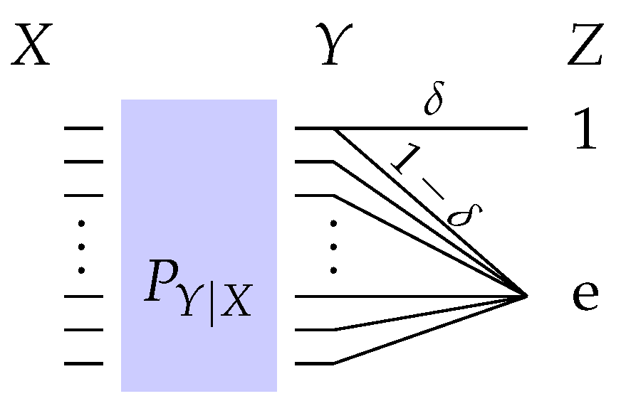
Appendix A. Proof of Lemma 19
Given a joint distribution defined over where and with , we consider a privacy filter specified by the following distribution for and
where denotes the indicator function. The system of in this case is depicted in Figure 6 for the case of .
We clearly have and , and hence
and also,
It, therefore, follows that for
and
We then write
and hence,
where
Using the first-order approximation of mutual information for , we can write
Similarly, we can write
where which yields
From the above, we obtain
Clearly from (A3), in order for the filter specified in (A1) and (A2) to belong to , we must have
and hence from (A4), we have
This immediately implies that
where we have used the assumption in the first equality.
Appendix B. Completion of Proof of Theorem 25
To prove that the equality (39) has only one solution , we first show the following lemma.
Lemma 33.
Let P and Q be two distributions over which satisfy . Let for . Then
for and
for .
Note that it is easy to see that the map is convex and strictly decreasing and hence when and when . Inequality (A6) and (A7) strengthen these monotonic behavior and show that and for and , respectively.
Proof.
Without loss of generality, we can assume that for all . Let , and . We notice that when , then , and hence for a . After relabelling if needed, we can therefore assume that and . We can write
where follows from the fact that for , for any , and in and we introduced and
Similarly, we can write
which implies that
Hence, in order to show (A6), it suffices to verify that
for any and . Since is always positive for , it suffices to show that
for and . We have
where
and
We have
because and hence . This implies that the map is concave for any and . Moreover, since is a quadratic polynomial with negative leading coefficient, it is clear that . Consider now . We have and for . It implies that is concave over and hence over which implies that . This together with the fact that is concave and it approaches to as imply that there exists a real number such that for all and for all . Since , it follows from (A10) that is convex over and concave over . Since and , we can conclude that over . That is, and thus , for and .
The inequality (A7) can be proved by (A6) and switching λ to . ☐
Letting and and , we have and . Since , we can conclude from Lemma 33 that
over and
over , and hence equation (39) has only solution .
Appendix C. Proof of Theorems 28 and 29
The proof of Theorem 29 does not depend on the proof of Theorem 28, so, there is no harm in proving the former theorem first. The following version of the data-processing inequality will be required.
Lemma 34.
Let X and Y be absolutely continuous random variables such that X, Y and have finite differential entropies. If V is an absolutely continuous random variable independent of X and Y, then
with equality if and only if X and Y are independent.
Proof.
Since , the data processing inequality implies that . It therefore suffices to show that this inequality is tight if and only X and Y are independent. It is known that data processing inequality is tight if and only if . This is equivalent to saying that for any measurable set and for almost all z, . On the other hand, due to the independence of V and , we have . Hence, the equality holds if and only if which implies that X and Y must be independent. ☐
Lemma 35.
In the notation of Section 5.1, the function is strictly-decreasing and continuous. Additionally, it satisfies
with equality if and only if Y is Gaussian. In particular, as .
Proof.
Recall that, by assumption b), is finite. The finiteness of the entropy of Y follows from assumption, the corresponding statement for follows from a routine application of the entropy power inequality [50, Theorem 17.7.3] and the fact that , and for the same conclusion follows by the chain rule for differential entropy. The data processing inequality, as stated in Lemma 34, implies
Clearly Y and are not independent, therefore the inequality is strict and thus is strictly-decreasing.
Continuity will be studied for and separately. Recall that . In particular, . The entropy power inequality shows then that . This coincides with the convention . For , let be a sequence of positive numbers such that . Observe that
Since , we only have to show that as to establish the continuity at γ. This, in fact, follows from de Bruijn’s identity (cf., [50, Theorem 17.7.2]).
Since the channel from Y to is an additive Gaussian noise channel, we have with equality if and only if Y is Gaussian. The claimed limit as is clear. ☐
Lemma 36.
The function is strictly-decreasing and continuous. Moreover, when .
Proof.
The proof of the strictly-decreasing behavior of is proved as in the previous lemma.
To prove continuity, let be fixed. Let be any sequence of positive numbers converging to γ. First suppose that . Observe that
for all . As shown in Lemma 35, as . Therefore, it is enough to show that as . Note that by de Bruijn’s identity, we have as for all . Note also that since
we can write
and hence we can apply dominated convergence theorem to show that as .
To prove the continuity at , we first note that Linder and Zamir [51, Page 2028] showed that as , then, as before, by dominated convergence theorem we can show that . Similarly [51] implies that . This concludes the proof of the continuity of .
Furthermore, by the data processing inequality and previous lemma,
and hence we conclude that . ☐
Proof of Theorem 29.
The nonnegativity of follows directly from definition.
By Lemma 36, for every there exists a unique such that , so . Moreover, is strictly decreasing. Since is strictly-decreasing, we conclude that is strictly increasing.
The fact that is strictly decreasing, also implies that as . In particular,
By the data processing inequality we have that for all , i.e., any filter satisfies the privacy constraint for . Thus, . ☐
In order to prove Theorem 28, we first recall the following theorem by Rényi [52].
Theorem 37
([52]). If U is an absolutely continuous random variable with density and if , then
provided that the integral on the right hand side exists.
We will need the following consequence of the previous theorem.
Lemma 38.
If U is an absolutely continuous random variable with density and if , then for all and
provided that the integral on the right hand side exists.
The previous lemma follows from the fact that is constructed by refining the quantization partition for .
Lemma 39.
For any ,
Proof.
Observe that
By the previous lemma, the integrand is decreasing in M, and thus we can take the limit with respect to M inside the integral. Thus,
The proof for is analogous. ☐
Lemma 40.
Fix . Assume that for some positive constant C and . For integer k and , let
Then
Proof.
The case is trivial, so we assume that . For notational simplicity, let for all . Assume that . Observe that
We will estimate the above integral by breaking it up into two pieces.
First, we consider
When , then . By the assumption on the density of Y,
(The previous estimate is the only contribution when .) Therefore,
Using the trivial bound and well known estimates for the error function, we obtain that
Therefore,
The proof for is completely analogous. ☐
Lemma 41.
Fix . Assume that for some positive constant C and . The mapping is continuous.
Proof.
Let be a sequence of non-negative real numbers converging to . First, we will prove continuity at . Without loss of generality, assume that for all . Define and . Clearly . Recall that
Since, for all and ,
the dominated convergence theorem implies that
The previous lemma implies that for all and ,
Thus, for k large enough, for a suitable positive constant A that does not depend on n. Since the function is increasing in , there exists such that for
Since , for any there exists such that
In particular, for all ,
Therefore, for all ,
By continuity of the function on and equation (A11), we conclude that
Since ϵ is arbitrary,
as we wanted to prove.
To prove continuity at , observe that equation (A11) holds in this case as well. The rest is analogous to the case . ☐
Lemma 42.
The functions and are continuous for each .
Proof.
Since and for are bounded by M, and satisfies assumption (b), the conclusion follows from the dominated convergence theorem. ☐
Proof of Theorem 28.
For every , let . The Markov chain and the data processing inequality imply that
and, in particular,
where is as defined in the proof of Theorem 29. This implies then that
and thus
Taking limits in both sides, Lemma 39 implies
Observe that
where inequality follows from Markovity and . By equation (A12), and in particular . Thus, is an increasing sequence in M and bounded from above and, hence, has a limit. Let . Clearly
By the previous lemma we know that is continuous, so is closed for all . Thus, we have that and in particular . By the inclusion , we have then that for all . By closedness of we have then that for all . In particular,
for all . By Lemma 39,
and by the monotonicity of , we obtain that . Combining the previous inequality with (A15) we conclude that . Taking limits in the inequality (A14)
Plugging in above we conclude that
and therefore . ☐
References
- Asoodeh, S.; Alajaji, F.; Linder, T. Notes on information-theoretic privacy. In Proceedings of the 52nd Annual Allerton Conference on Communication, Control, and Computing, Monticello, IL, USA, 30 September–3 October 2014; pp. 1272–1278.
- Asoodeh, S.; Alajaji, F.; Linder, T. On maximal correlation, mutual information and data privacy. In Proceedings of the IEEE 14th Canadian Workshop on Information Theory (CWIT), St. John’s, NL, Canada, 6–9 July 2015; pp. 27–31.
- Warner, S.L. Randomized Response: A Survey Technique for Eliminating Evasive Answer Bias. J. Am. Stat. Assoc. 1965, 60, 63–69. [Google Scholar] [CrossRef] [PubMed]
- Blum, A.; Ligett, K.; Roth, A. A learning theory approach to non-interactive database privacy. In Proceedings of the Fortieth Annual ACM Symposium on the Theory of Computing, Victoria, BC, Canada, 17–20 May 2008; pp. 1123–1127.
- Dinur, I.; Nissim, K. Revealing information while preserving privacy. In Proceedings of the Twenty-Second Symposium on Principles of Database Systems, San Diego, CA, USA, 9–11 June 2003; pp. 202–210.
- Rubinstein, P.B.; Bartlett, L.; Huang, J.; Taft, N. Learning in a large function space: Privacy-preserving mechanisms for SVM learning. J. Priv. Confid. 2012, 4, 65–100. [Google Scholar]
- Duchi, J.C.; Jordan, M.I.; Wainwright, M.J. Privacy aware learning. 2014; arXiv: 1210.2085. [Google Scholar]
- Dwork, C.; McSherry, F.; Nissim, K.; Smith, A. Calibrating noise to sensitivity in private data analysis. In Proceedings of the Third Conference on Theory of Cryptography (TCC’06), New York, NY, USA, 5–7 March 2006; pp. 265–284.
- Dwork, C. Differential privacy: A survey of results. In Theory and Applications of Models of Computation, Proceedings of the 5th International Conference, TAMC 2008, Xi’an, China, 25–29 April 2008; Agrawal, M., Du, D., Duan, Z., Li, A., Eds.; Springer: Berlin/Heidelberg, Germany, 2008. Lecture Notes in Computer Science. Volume 4978, pp. 1–19. [Google Scholar]
- Dwork, C.; Lei, J. Differential privacy and robust statistics. In Proceedings of the 41st Annual ACM Symposium on the Theory of Computing, Bethesda, MD, USA, 31 May–2 June 2009; pp. 437–442.
- Kairouz, P.; Oh, S.; Viswanath, P. Extremal mechanisms for local differential privacy. 2014; arXiv: 1407.1338v2. [Google Scholar]
- Calmon, F.P.; Varia, M.; Médard, M.; Christiansen, M.M.; Duffy, K.R.; Tessaro, S. Bounds on inference. In Proceedings of the 51st Annual Allerton Conference on Communication, Control, and Computing, Monticello, IL, USA, 2–4 October 2013; pp. 567–574.
- Yamamoto, H. A source coding problem for sources with additional outputs to keep secret from the receiver or wiretappers. IEEE Trans. Inf. Theory 1983, 29, 918–923. [Google Scholar] [CrossRef]
- Sankar, L.; Rajagopalan, S.; Poor, H. Utility-privacy tradeoffs in databases: An information-theoretic approach. IEEE Trans. Inf. Forensics Secur. 2013, 8, 838–852. [Google Scholar] [CrossRef]
- Tandon, R.; Sankar, L.; Poor, H. Discriminatory lossy source coding: side information privacy. IEEE Trans. Inf. Theory 2013, 59, 5665–5677. [Google Scholar] [CrossRef]
- Calmon, F.; Fawaz, N. Privacy against statistical inference. In Proceedings of the 50th Annual Allerton Conference on Communication, Control, and Computing, Monticello, IL, USA, 1–5 October 2012; pp. 1401–1408.
- Rebollo-Monedero, D.; Forne, J.; Domingo-Ferrer, J. From t-closeness-like privacy to postrandomization via information theory. IEEE Trans. Knowl. Data Eng. 2010, 22, 1623–1636. [Google Scholar] [CrossRef] [Green Version]
- Makhdoumi, A.; Salamatian, S.; Fawaz, N.; Médard, M. From the information bottleneck to the privacy funnel. In Proceedings of the IEEE Information Theory Workshop (ITW), Hobart, Australia, 2–5 November 2014; pp. 501–505.
- Tishby, N.; Pereira, F.C.; Bialek, W. The information bottleneck method. 2000; arXiv: physics/0004057. [Google Scholar]
- Calmon, F.P.; Makhdoumi, A.; Médard, M. Fundamental limits of perfect privacy. In Proceedings of the IEEE Int. Symp. Inf. Theory (ISIT), Hong Kong, China, 14–19 June 2015; pp. 1796–1800.
- Wyner, A.D. The Wire-Tap Channel. Bell Syst. Tech. J. 1975, 54, 1355–1387. [Google Scholar] [CrossRef]
- Makhdoumi, A.; Fawaz, N. Privacy-utility tradeoff under statistical uncertainty. In Proceedings of the 51st Annual Allerton Conference on Communication, Control, and Computing, Monticello, IL, USA, 2–4 October 2013; pp. 1627–1634.
- Li, C.T.; El Gamal, A. Maximal correlation secrecy. 2015; arXiv: 1412.5374. [Google Scholar]
- Ahlswede, R.; Gács, P. Spreading of sets in product spaces and hypercontraction of the Markov operator. Ann. Probab. 1976, 4, 925–939. [Google Scholar] [CrossRef]
- Anantharam, V.; Gohari, A.; Kamath, S.; Nair, C. On maximal correlation, hypercontractivity, and the data processing inequality studied by Erkip and Cover. 2014; arXiv:1304.6133v1. [Google Scholar]
- Courtade, T. Information masking and amplification: The source coding setting. In Proceedings of the IEEE Int. Symp. Inf. Theory (ISIT), Boston, MA, USA, 1–6 July 2012; pp. 189–193.
- Goldwasser, S.; Micali, S. Probabilistic encryption. J. Comput. Syst. Sci. 1984, 28, 270–299. [Google Scholar] [CrossRef]
- Rockafellar, R.T. Convex Analysis; Princeton Univerity Press: Princeton, NJ, USA, 1997. [Google Scholar]
- Csiszár, I.; Körner, J. Information Theory: Coding Theorems for Discrete Memoryless Systems; Cambridge University Press: Cambridge, UK, 2011. [Google Scholar]
- Shulman, N.; Feder, M. The uniform distribution as a universal prior. IEEE Trans. Inf. Theory 2004, 50, 1356–1362. [Google Scholar] [CrossRef]
- Rudin, W. Real and Complex Analysis, 3rd ed.; McGraw Hill: New York, NY, USA, 1987. [Google Scholar]
- Gebelein, H. Das statistische Problem der Korrelation als Variations- und Eigenwert-problem und sein Zusammenhang mit der Ausgleichungsrechnung. Zeitschrift f ur Angewandte Mathematik und Mechanik 1941, 21, 364–379. (In German) [Google Scholar] [CrossRef]
- Hirschfeld, H.O. A connection between correlation and contingency. Camb. Philos. Soc. 1935, 31, 520–524. [Google Scholar] [CrossRef]
- Rényi, A. On measures of dependence. Acta Mathematica Academiae Scientiarum Hungarica 1959, 10, 441–451. [Google Scholar] [CrossRef]
- Linfoot, E.H. An informational measure of correlation. Inf. Control 1957, 1, 85–89. [Google Scholar] [CrossRef]
- Csiszár, I. Information-type measures of difference of probability distributions and indirect observation. Studia Scientiarum Mathematicarum Hungarica 1967, 2, 229–318. [Google Scholar]
- Zhao, L. Common Randomness, Efficiency, and Actions. Ph.D. Thesis, Stanford University, Stanford, CA, USA, 2011. [Google Scholar]
- Berger, T.; Yeung, R. Multiterminal source encoding with encoder breakdown. IEEE Trans. Inf. Theory 1989, 35, 237–244. [Google Scholar] [CrossRef]
- Kim, Y.H.; Sutivong, A.; Cover, T. State mplification. IEEE Trans. Inf. Theory 2008, 54, 1850–1859. [Google Scholar] [CrossRef]
- Merhav, N.; Shamai, S. Information rates subject to state masking. IEEE Trans. Inf. Theory 2007, 53, 2254–2261. [Google Scholar] [CrossRef]
- Ahlswede, R.; Körner, J. Source coding with side information and a converse for degraded broadcast channels. IEEE Trans. Inf. Theory 1975, 21, 629–637. [Google Scholar] [CrossRef]
- Kim, Y.H.; El Gamal, A. Network Information Theory; Cambridge University Press: Cambridge, UK, 2012. [Google Scholar]
- Asoodeh, S.; Alajaji, F.; Linder, T. Lossless secure source coding, Yamamoto’s setting. In Proceedings of the 53rd Annual Allerton Conference on Communication, Control, and Computing, Monticello, IL, USA, 30 September–2 October 2015.
- Raginsky, M. Logarithmic Sobolev inequalities and strong data processing theorems for discrete channels. In Proceedings of the IEEE Int. Sym. Inf. Theory (ISIT), Istanbul, Turkey, 7–12 July 2013; pp. 419–423.
- Geng, Y.; Nair, C.; Shamai, S.; Wang, Z.V. On broadcast channels with binary inputs and symmetric outputs. IEEE Trans. Inf. Theory 2013, 59, 6980–6989. [Google Scholar] [CrossRef]
- Sutskover, I.; Shamai, S.; Ziv, J. Extremes of information combining. IEEE Trans. Inf. Theory 2005, 51, 1313–1325. [Google Scholar] [CrossRef]
- Alajaji, F.; Chen, P.N. Information Theory for Single User Systems, Part I. Course Notes, Queen’s University. Available online: http://www.mast.queensu.ca/math474/it-lecture-notes.pdf (accessed on 4 March 2015).
- Chayat, N.; Shamai, S. Extension of an entropy property for binary input memoryless symmetric channels. IEEE Trans.Inf. Theory 1989, 35, 1077–1079. [Google Scholar] [CrossRef]
- Oohama, Y. Gaussian multiterminal source coding. IEEE Trans. Inf. Theory 1997, 43, 2254–2261. [Google Scholar] [CrossRef]
- Cover, T.M.; Thomas, J.A. Elements of Information Theory; Wiley: New York, NY, USA, 2006. [Google Scholar]
- Linder, T.; Zamir, R. On the asymptotic tightness of the Shannon lower bound. IEEE Trans. Inf. Theory 2008, 40, 2026–2031. [Google Scholar] [CrossRef]
- Rényi, A. On the dimension and entropy of probability distributions. cta Mathematica Academiae Scientiarum Hungarica 1959, 10, 193–215. [Google Scholar] [CrossRef]
Figure 1.
Information-theoretic privacy.
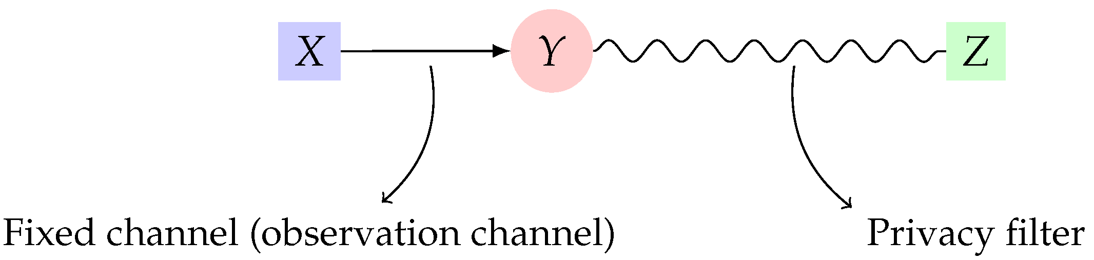
Figure 2.
Privacy filter that achieves the lower bound in (4) where is the output of an erasure privacy filter with erasure probability specified in (5).
Figure 2.
Privacy filter that achieves the lower bound in (4) where is the output of an erasure privacy filter with erasure probability specified in (5).
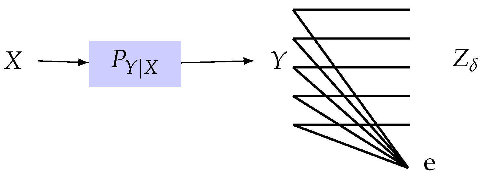
Figure 3.
The region of in terms of ε specified by (4).
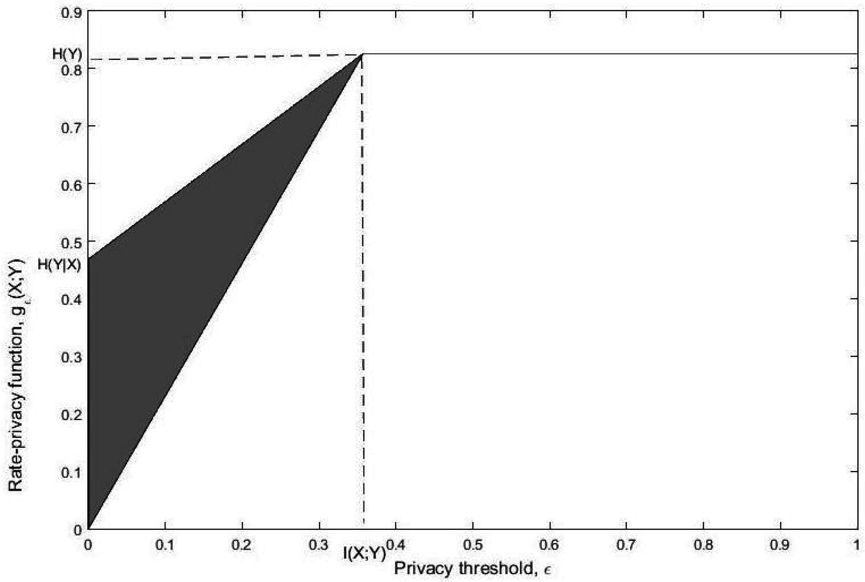
Figure 4.
Optimal privacy filter for with uniform X where is specified in (40).

Figure 5.
Optimal privacy filter for where is specified in (42).
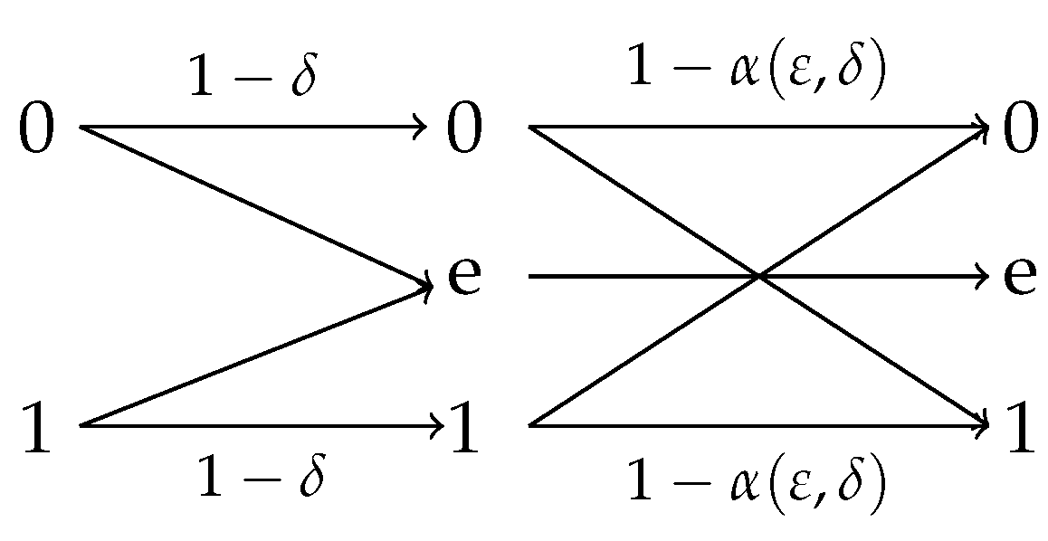
Figure 6.
The privacy filter associated with (A1) and (A2) with . We have and for .
© 2016 by the authors; licensee MDPI, Basel, Switzerland. This article is an open access article distributed under the terms and conditions of the Creative Commons by Attribution (CC-BY) license (http://creativecommons.org/licenses/by/4.0/).
Share and Cite
MDPI and ACS Style
Asoodeh, S.; Diaz, M.; Alajaji, F.; Linder, T. Information Extraction Under Privacy Constraints. Information 2016, 7, 15. https://doi.org/10.3390/info7010015
AMA Style
Asoodeh S, Diaz M, Alajaji F, Linder T. Information Extraction Under Privacy Constraints. Information. 2016; 7(1):15. https://doi.org/10.3390/info7010015
Chicago/Turabian StyleAsoodeh, Shahab, Mario Diaz, Fady Alajaji, and Tamás Linder. 2016. "Information Extraction Under Privacy Constraints" Information 7, no. 1: 15. https://doi.org/10.3390/info7010015
Note that from the first issue of 2016, this journal uses article numbers instead of page numbers. See further details here.