Bayesian Angular Superresolution Algorithm for Real-Aperture Imaging in Forward-Looking Radar

Abstract

In real aperture imaging, the limited azimuth angular resolution seriously restricts the applications of this imaging system. This report presents a maximum a posteriori (MAP) approach based on the Bayesian framework for high angular resolution of real aperture radar. First, Rayleigh statistic and the $l_q$ norm (for $0<q\le 1$) sparse constraint are considered to express the clutter property and target scattering coefficient distribution, respectively. Then, the MAP objective function is established according to the hypotheses above. At last, a recursive iterative strategy is developed to estimate the original target scattering coefficient distribution and clutter statistic. The comparison of simulations and experimental results are given to verify the performance of our proposed algorithm.

1. Introduction

Real aperture imaging is a noncoherent imaging system, which is suitable for any geometry situation. This imaging system can be widely used in many applications, such as environmental monitoring and disaster rescue. In a real aperture scanning radar system, we usually transmit the linear frequency modulation (LFM) for high resolution in the range dimension [1]. However, in the azimuth dimension, the angular resolution is determined by the real aperture width and antenna wavelength. Few techniques can break the limitation of antenna aperture to realize high azimuth resolution. The low azimuth angular resolution seriously influences the application of this imaging system [2]. It is significant for us to propose effective methods to improve the azimuth angular resolution.

Recently, some approaches have been proposed to enhance the spatial resolution [3,4,5,6,7,8,9,10]. In [9,10], the researchers introduced the spectrum estimation methods to enhance the azimuth angular resolution of a real aperture image. However, how to collect enough snapshots to realize the high estimation precision of the covariance matrix is difficult for the mechanical scanning radar system. The iterative adaptive approach (IAA) is a novel approach that could significantly decrease the requirement of snapshots [11,12,13]. Some effects have been obtained by applying this approach to the the real aperture angular superresolution problem [14,15]. However, the computational complexity of this algorithm is too high for practical applications. The truncated singular value decomposition (TSVD) is an effective reconstruction method for the high spatial resolution of radiometer data [16,17,18,19]. The basic idea of TSVD is to truncate the SVD solution to discard the components dominated by noise. This method can be extended to the real aperture imaging problem for the superresolution of both the range dimension and the azimuth dimension.

Another class of deconvolution algorithms is based on the Bayesian framework. It has been developed and successfully applied to the high-resolution problem of radar imaging, including SAR imaging, MIMO signal processing, etc. [20,21,22]. In these references above, the maximum a posteriori (MAP) algorithm was proposed based on the assumptions that the statistic of noise obeys a Gaussian or a Poisson distribution. Besides, prior information was used for high angular resolution and image quality. Tikhonov regularization is a classic regularization method that uses the Euclidean norm to realize resolution enhancement and denoising [23,24]. In addition, the sparse constraint was usually considered as the prior information of the target distribution in real aperture imaging because the major application of real aperture radar is to obtain the amplitude and position information of a strong scattering target, and in most cases, the distribution of the strong scattering target is sparse relative to the imaging area. Furthermore, using the sparse constraint also could reduce the impact of noise amplification, which is one of the major drawbacks of the Bayesian deconvolution method. The $l_1$ norm is the most common sparse constraint in sparse signal recovery algorithms; however, some recent research shows that other sparse constraints could also realize high signal recovery performance. In [25], it has been proven that the $l_q$ norm (for $0<q\le 1$) -based technique gave a sparser and more accurate estimation result than the $l_1$ norm-based technique. It also has been demonstrated by the simulation results of MIMO and SAR imaging that this sparsity-promoting constraint provided better signal recovery capability than the $l_1$ norm-based technique [20,26]. Therefore, we introduce this sparse constraint to real aperture imaging for high angular superresolution performance.

In the present report, we first adopt the Rayleigh statistic to describe the amplitude characteristic of clutter for the following two reasons: (1) according to the central limit theorem, it has been assumed that the real and the imaginary parts of the received signals follow a Gaussian distribution, which in turn, leads to the Rayleigh distribution as the amplitude distribution model [27]; (2) this distribution has been employed to describe the clutter property of some natural scenes, such as the sea surface when imaged by a coarse resolution radar or when the long wave structure is negligible [28,29]. Then, the mentioned $l_p$ norm sparse constraint is considered as the prior information of the scattering target distribution. Finally, a recursive iterative strategy is developed to estimate the unknown statistic parameter of the Rayleigh distribution and to recover the original target distribution.

This report is organized as follows: In Section 2, we will begin our discussion by introducing the real aperture signal model. In Section 3, the Tikhonov regularization method and Richardson-Lucy (RL) algorithm are introduced first. Then, the MAP objective function of the proposed algorithm is established according to the hypothesized distributions of the clutter and target. In addition, the derivation of the objective function is described in detail. In Section 4, some simulations and real measured data are offered for the comparison of the proposed MAP algorithm with two traditional deconvolution techniques. Conclusions are given in Section 5.

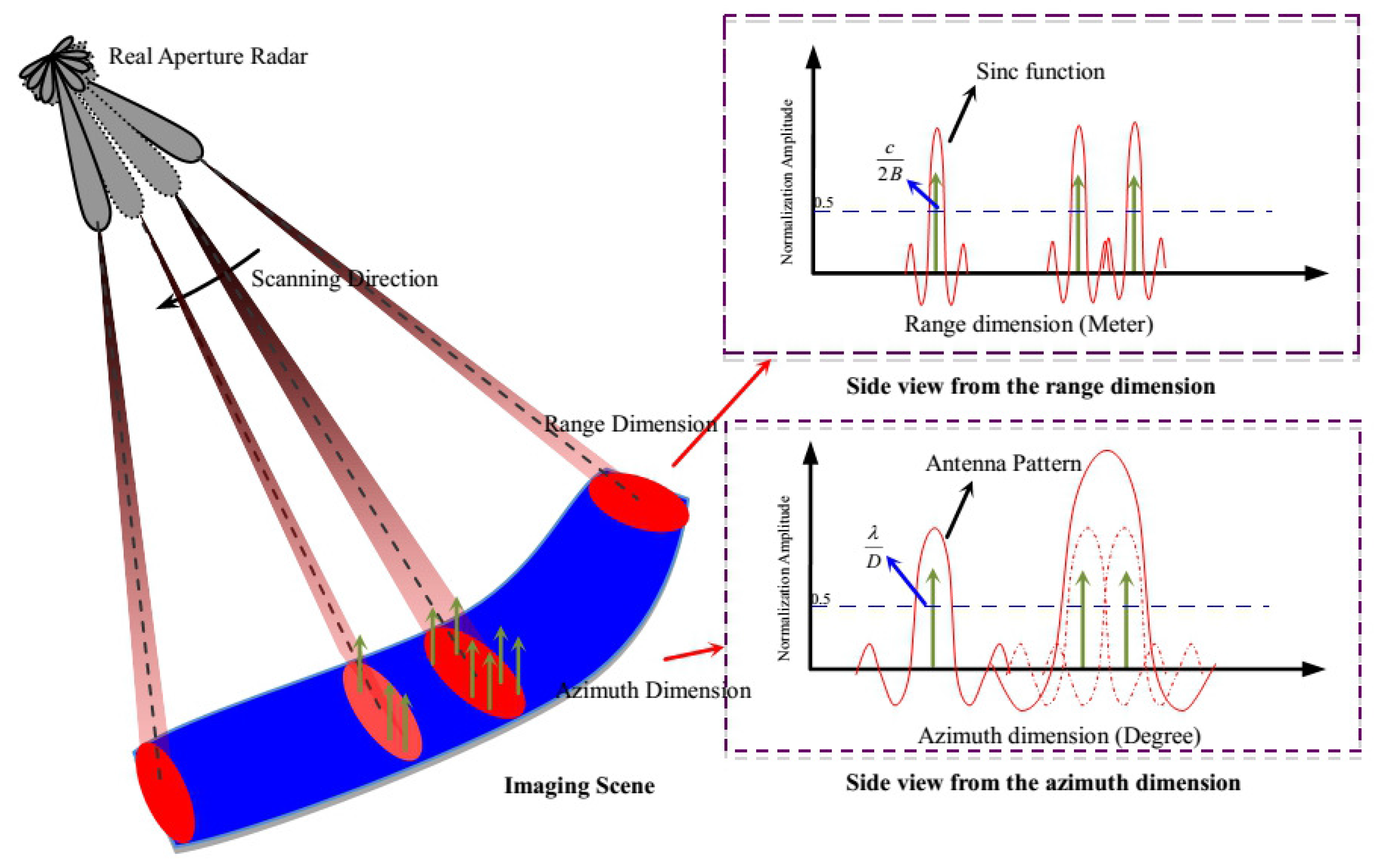
2. Signal Model of the Real Aperture Image

Figure 1 shows the working model of the real aperture scanning radar.

Figure 1. Geometric model of the real aperture scanning radar.

Figure 1. Geometric model of the real aperture scanning radar.

The antenna transmits LFM signals and sweeps across the detection scene with clockwise mechanical movement. Some targets are located at the detection scene with different range positions and azimuth angular variables. The received echo can be written as the following two-dimensional convolution model after the operation of pulse compression in the range dimension:

$$s\left(r,\theta \right)=h\left(r,\theta \right)\otimes f\left(r,\theta \right)$$

(1)

where ⊗ is the convolution operator, $s\left(r,\theta \right)$ is the received two-dimensional signal, r and θ represent the range and angular variable of the two-dimensional signal, respectively, $h\left(r,\theta \right)$ is the two-dimensional convolution kernel function and $f\left(r,\theta \right)$ is the target scattering distribution. In the range dimension, the convolution kernel function is the the $sinc$ function, and the range resolution is defined as the 3-dB width of the $sinc$ function, which can be calculated by $c/\phantom{c2B}2B$, where c is the velocity of microwave transmitting and B is the bandwidth of the transmitted signal. We can easily achieve high range resolution by transmitting a large bandwidth signal. However, in the azimuth dimension, the convolution kernel function is the antenna pattern, and the azimuth angular resolution is determined by $\lambda /\phantom{\lambda D}D$, where λ is the wavelength of the carrier signal and D is the size of the antenna aperture. For the typical antenna and working distance, the azimuth resolution is much less than the range resolution. This report presents a novel deconvolution method for high azimuth angular resolution. The received real aperture signal of the observation range profiles could be expressed in matrix form as:

$$\begin{array}{cc}\hfill \mathbf{s}& =\mathbf{Hf}+\mathbf{n}\hfill \\ & =\left[\begin{array}{ccc}{H}_{M\times M}& & \\ & \ddots & \\ & & H_{M\times M}\end{array}\right]\left[\begin{array}{c}\begin{array}{c}f\left(1,1\right)\hfill \\ f\left(1,2\right)\hfill \end{array}\\ ⋮\\ f\left(N,1\right)\\ \begin{array}{c}⋮\hfill \\ f\left(N,M\right)\hfill \end{array}\end{array}\right]+\mathbf{n}\hfill \end{array}$$

(2)

where $\mathbf{s}$ and $\mathbf{f}$ represent the measurement range profiles and unknown target amplitude profiles, which are rearranged in the azimuth dimension with size $NM\times 1$, N is the discrete sampling number of the range dimension, which can be calculated by:

$$N=\left(R/\phantom{Rc}c+2·T\right)·frs$$

(3)

where R denotes the imaging area of range dimension, c denotes the speed of light, T denotes the time width of transmitted signal and $frs$ denotes the sampling frequency of the range dimension. The discrete sampling number in the azimuth dimension is:

$$M=PRF·\phi /\phantom{\phi \omega }\omega$$

(4)

where $PRF$ denotes the pulse repetition frequency of the transmitted signal, φ denotes the scanning area in the azimuth dimension and ω denotes the scanning speed. Because the number of strong scattering targets is sparse relative to the dimension of the received echo in most cases, therefore most elements of $\mathbf{f}$ are supposed to be zero, and the sparse constraint can be considered as the prior information for superior angular resolution. Vector $\mathbf{n}$ represents the clutter profiles, which are rearranged in the azimuth dimension with dimension $NM\times 1$, and the amplitude of this clutter vector obeys the independent Rayleigh distribution with unknown statistic parameter σ. In the next section, we propose a recursive strategy to accurately estimate this unknown parameter for high angular superresolution performance. Matrix $\mathbf{H}$ is the rearranged measurement matrix with size $NM\times NM$. This matrix is composed of convolution matrix $H_{M\times M}$, and $H_{M\times M}=\left[{\mathbf{h}}_1,{\mathbf{h}}_2,\cdots ,{\mathbf{h}}_M\right]$ is the convolution measurement matrix of the single range unit, which can be written as:

$${\mathbf{H}}_{M\times M}=\left[\begin{array}{ccccc}{h}_1& h_M& h_{M-1}& \cdots & h_2\\ h_2& h_1& h_M& \cdots & h_3\\ h_3& h_2& h_1& \cdots & h_4\\ ⋮& ⋮& ⋮& & ⋮\\ h_M& h_{M-1}& h_{M-2}& \cdots & h_1\end{array}\right]$$

(5)

where the elements of Equation (3) are the weighted value of the antenna pattern to the corresponding target at different sampling times. Equation (2) could be regarded as the classical signal recovery problem in estimation theory. In the next section, the MAP deconvolution algorithm is proposed based on the practical property of the clutter and target.

3. Angular Superresolution for Real Aperture Radar

In this section, we first introduce two traditional superresolution methods and discuss the shortcomings if we directly apply these methods to the real aperture imaging. Then, we propose the MAP deconvolution method based on the Bayesian framework.

3.1. Tikhonov Regularization

Tikhonov’s method solves the problem Equation (2) based on least squares (LS) estimation, with Euclidean norms. A common version of Tikhonov’s method takes the form:

$$\begin{array}{c}\hfill \underset{\mathbf{f}}{min}\left\{{∥\mathbf{Hf}-\mathbf{s}∥}_2^2+\lambda {∥\mathbf{f}∥}_2^2\right\}\end{array}$$

(6)

where λ is a positive constant, which controls the trade-off the residual between ${∥\mathbf{Hf}-\mathbf{s}∥}_2^2$ and ${∥\mathbf{f}∥}_2^2$. This Tikhonov regularization problem has the analytical solution:

$$\begin{array}{c}\hfill \mathbf{f}={\left({\mathbf{H}}^T\mathbf{H}+\lambda \mathbf{I}\right)}^{-1}{\mathbf{H}}^T\mathbf{s}\end{array}$$

(7)

This method has limited performance for azimuth angular resolution. Besides, this method needs to do a balance between image quality and resolution in low signal-to-clutter ratio (SCR) condition. It improves the azimuth angular solution at the cost of image quality.

3.2. Richardson-Lucy Superresolution Algorithm

The Richardson-Lucy (RL) algorithm is a classic maximum likelihood (ML) superresolution approach based on Bayesian framework. This algorithm has been widely used in optical imaging and confocal microscope imaging for many years [30,31]. Recently, some references introduced this algorithm to radar signal processing to enhance the azimuth angular resolution of the scanning radar [22].

The MAP estimation is to solve the following problem:

$$\begin{array}{c}\hfill \begin{array}{cc}\hfill \widehat{\mathbf{f}}& =arg\underset{\mathbf{f}}{max}p\left(\mathbf{f}/\phantom{\mathbf{f}\mathbf{s}}\mathbf{s}\right)=arg\underset{\mathbf{f}}{max}p\left(\mathbf{s}/\phantom{\mathbf{s}\mathbf{f}}\mathbf{f}\right)p\left(\mathbf{f}\right)\hfill \\ & =arg\underset{\mathbf{f}}{min}\left\{-lnp\left(\mathbf{s}/\phantom{\mathbf{s}\mathbf{f}}\mathbf{f}\right)-lnp\left(\mathbf{f}\right)\right\}\hfill \end{array}\end{array}$$

(8)

where $p\left(\mathbf{f}/\phantom{\mathbf{s}\mathbf{f}}\mathbf{s}\right)$ is the a posteriori probability and $p\left(\mathbf{s}/\phantom{\mathbf{f}\mathbf{s}}\mathbf{f}\right)$ is the likelihood probability, $p\left(\mathbf{f}\right)$ is the prior knowledge of the target. Using the negative logarithm operation is convenient for the calculations.

The RL algorithm based on the assumptions that the noise in each observed cells is independent and obeys the Poisson distribution. Besides, it is assumed that the target scattering coefficient obeys the uniform distribution that makes the MAP estimation equal to the ML estimation:

$$\widehat{\mathbf{f}}=arg\underset{\mathbf{f}}{max}p\left(\mathbf{f}/\phantom{\mathbf{f}\mathbf{s}}\mathbf{s}\right)=arg\underset{\mathbf{f}}{max}p\left(\mathbf{s}/\phantom{\mathbf{s}\mathbf{f}}\mathbf{f}\right)=arg\underset{\mathbf{f}}{min}\left\{-lnp\left(\mathbf{s}/\phantom{\mathbf{s}\mathbf{f}}\mathbf{f}\right)\right\}$$

(9)

Now, the objective function can be written as:

$$p\left(\mathbf{s}/\phantom{\mathbf{s}\mathbf{f}}\mathbf{f}\right)=\prod _{i=1}^{NM}\frac{{{\left(Hf\right)}_i}^{s_i}exp\left(-{\left(Hf\right)}_i\right)}{\left(s_i\right)!}$$

(10)

where i is the sampling cell, ${\left(Hf\right)}_i={\displaystyle \sum _{j=1}^{NM}}{h}_{ij}{f}_j$. After the negative logarithm operation, the objective function becomes:

$$J\left(\mathbf{f}\right)=-lnp\left(\mathbf{s}/\phantom{\mathbf{s}\mathbf{f}}\mathbf{f}\right)=\sum _i\{{\left(Hf\right)}_i+ln[s_i!]-s_{i}ln\left[{\left(Hf\right)}_i\right]\}$$

(11)

We can obtain the ML solution by setting the gradient of $J\left(\mathbf{f}\right)$ to zero, with $\sum \mathbf{h}\left(i\right)=1$:

$$\begin{array}{c}\hfill {\mathbf{H}}^T\left(\frac{\mathbf{s}}{\mathbf{Hf}}\right)=1\end{array}$$

(12)

where ${\left(·\right)}^T$ means the transposed matrix. Then, the RL algorithm adopts a multiplicative iterative method to obtain the following iterative expression:

$$\begin{array}{c}\hfill {\mathbf{f}}_{k+1}={\mathbf{f}}_k\left[{\mathbf{H}}^T\left(\frac{\mathbf{s}}{\mathbf{H}{\mathbf{f}}_k}\right)\right]\end{array}$$

(13)

where $k+1$ and k are the iterations. Although this algorithm obtained some effects in radar imaging, the assumption that noise obeys a Poisson distribution does not satisfy the actual noise or clutter characteristic. Besides, the phenomena of image distortion and noise amplification cannot be avoided in the low SNR condition, because little prior information of target is considered in this algorithm.

3.3. Proposed MAP Deconvolution Algorithm

In the proposed algorithm, we adopt the Rayleigh statistic to express the distribution property of the clutter amplitude. For the model of speckle and clutter in SAR and the sea clutter image, we consider that a resolution cell is composed of many independent scatterers, and each scatterer obeys an independent, zero mean, identically complex Gaussian distribution [32,33]. Therefore, the amplitude of each resolution cell obeys the Rayleigh distribution according to the central limit theorem. In the common application of a real aperture system, the footprint is sufficiently large to contain many independent scatterers. Therefore, we assume that the amplitude of the clutter at each sampling cell obeys an independent Rayleigh distribution. The likelihood probability can be written as:

$$\begin{array}{c}\hfill p\left(\mathbf{s}/\mathbf{f}\right)=\prod _{i=1}^{NM}\frac{\left(s_i-{\left(Hf\right)}_i\right)}{{\sigma }^2}{e}^{\left(-\frac{{\left(s_i-{\left(Hf\right)}_i\right)}^2}{2{\sigma }^2}\right)}\end{array}$$

(14)

In this report, the sparse constraint is considered as the prior information of the target distribution in the following three aspects: First, a major goal of angular superresolution is to realize the precision estimation of a strong scattering target. Second, the distribution of the strong scattering target is sparse relative to the imaging area in most applications of real aperture imaging. At last, when the sampling number is less than the target number in the azimuth dimension, the sparse constraint still applies. Therefore, the proposed algorithm employs the following sparse constraint as the prior information:

$$p\left(\mathbf{f}\right)\propto \prod _{i=1}^{NM}exp\left[-\frac{2}{q}\left({\left|f_i\right|}^q-1\right)\right]$$

(15)

where $0<q\le 1$. When $q=1$, $p\left(\mathbf{f}\right)\propto exp\left(-2{∥\mathbf{f}∥}_1\right)$ becomes Laplace distribution. Now, the algorithm can be regarded as the Rayleigh-based $l_1$ norm deconvolution algorithm. When $q\to 0$, the prior term becomes $p\left(\mathbf{f}\right)\propto {\displaystyle \prod _{i=1}^{NM}}\left(1/\phantom{1{\left|f_i\right|}^2}{\left|f_i\right|}^2\right)$. In general, the prior corresponding to a smaller q has a sharper peak at zero and provides sparser estimates in Bayesian inference. It has been proven that this sparse constraint provides better signal recovery performance than the $l_1$ norm constraint in MIMO and SAR imaging [20,26]. Substituting Equations (14) and (15) into Equation (8), the MAP objective function is:

$$\begin{array}{c}\hfill \begin{array}{c}\hfill g\left(\mathbf{f}\right)=p\left(\mathbf{s}/\phantom{\mathbf{s}\mathbf{f}}\mathbf{f}\right)p\left(\mathbf{f}\right)=\prod _{i=1}^{NM}\frac{\left(s_i-{\left(Hf\right)}_i\right)}{{\sigma }^2}{e}^{\left(-\frac{{\left(s_i-{\left(Hf\right)}_i\right)}^2}{2{\sigma }^2}\right)}·\prod _{i=1}^{NM}exp\left[-\frac{2}{q}\left({\left|f_i\right|}^q-1\right)\right]\end{array}\end{array}$$

(16)

By using the negative logarithm operation, the objective function becomes:

$$\begin{array}{c}\hfill \begin{array}{cc}\hfill \phi \left(\mathbf{f}\right)=-lng\left(\mathbf{f}\right)=& \sum _{i=1}^{NM}\left[-ln\left(s_i-{\left(Hf\right)}_i\right)+\frac{{\left(s_i-{\left(Hf\right)}_i\right)}^2}{2{\sigma }^2}\right]+NMln{\sigma }^2\hfill \\ & +\sum _{i=1}^{NM}\frac{2}{q}\left({\left|x_n\right|}^q-1\right)\hfill \end{array}\end{array}$$

(17)

where the statistic parameter of Rayleigh distribution is unknown. We employ the maximum likelihood estimation (MLE) to estimate it first [34]. Letting $g_1,\cdots ,g_i$ be a sampling series of sea clutter data with size $NM$, the log-likelihood function of Rayleigh distribution can be written as:

$$\begin{array}{c}\hfill \gamma \left(\mathbf{g},\sigma \right)=NMln{\sigma }^2-\sum _{i=1}^{NM}{g}_i+\sum _{i=1}^{NM}\frac{{\left(g_i\right)}^2}{2{\sigma }^2}\end{array}$$

(18)

Then, we compute the gradient of (18) with respect to σ:

$$\begin{array}{c}\hfill \frac{\partial \left(\gamma \left(\mathbf{g},\sigma \right)\right)}{\partial \sigma }=\frac{2NM}{\sigma }-\frac{1}{{\sigma }^3}\sum _{i=1}^{NM}{\left(g_i\right)}^2=0\end{array}$$

(19)

The MLE of ${\sigma }^2$ is:

$$\begin{array}{c}\hfill {\sigma }^2=\frac{{\displaystyle \sum _{i=1}^{NM}}{\left(g_i\right)}^2}{2NM}\end{array}$$

(20)

In real aperture imaging, $g_i$ can be replaced by $s_i-{\left(Hf\right)}_i$. Now, Equation (20) becomes:

$$\begin{array}{c}\hfill {\sigma }^2=\frac{{\displaystyle \sum _{i=1}^{NM}}{\left(s_i-{\left(Hf\right)}_i\right)}^2}{2NM}\end{array}$$

(21)

We can substitute the coarse initial iterative value of $\mathbf{f}$ to calculate ${\sigma }^2$. However, this operation may cause the serious estimation error of the original target distribution. Here, we adopt a recursive iterative strategy for high estimation accuracy. First, we calculate the gradient of (17) with respect to $\mathbf{f}$:

$$\begin{array}{c}\hfill \begin{array}{c}\hfill \nabla \phi \left(\mathbf{f}\right)={\mathbf{H}}^T\frac{1}{\mathbf{s}-\mathbf{Hf}}-\frac{1}{{\sigma }^2}{\mathbf{H}}^T\left(\mathbf{s}-\mathbf{Hf}\right)+{\mathbf{P}}^{-\mathbf{1}}\mathbf{f}\end{array}\end{array}$$

(22)

where $\mathbf{P}=diag\left\{p_1,\cdots ,p_{NM}\right\}$ and $p_i={\left|f_i\right|}^{2-q}$. We can now minimize Equation (22) by letting $\nabla \phi \left(\mathbf{f}\right)=0$. Then, we solve for $\mathbf{f}$ by a iterative strategy, because Equation (22) is a nonlinear function. The simple solution of Equation (22) is:

$$\begin{array}{c}\hfill \mathbf{f}={\left({\mathbf{H}}^T\mathbf{H}+{\sigma }^2{\mathbf{P}}^{-1}\right)}^{-1}\left({\mathbf{H}}^T\mathbf{s}-{\sigma }^2{\mathbf{H}}^T\frac{1}{\mathbf{s}-\mathbf{Hf}}\right)\end{array}$$

(23)

Now, we substitute the initial values of $\mathbf{f}$ and ${\sigma }^2$, which were computed by the coarse least square estimation (LSE) and maximum likelihood estimation (MLE) into Equation (23), to compute a new solution. The new estimation is also substituted into Equation (21) to update ${\sigma }^2$. Equations (21) and (23) to construct the recursive iterative strategy. The iterative expression is:

$$\begin{array}{c}\hfill {\mathbf{f}}_{k+1}={\left({\mathbf{H}}^T\mathbf{H}+{\left({\sigma }^2\right)}_k{\left({\mathbf{P}}_k\right)}^{-1}\right)}^{-1}\left({\mathbf{H}}^T\mathbf{s}-{\left({\sigma }^2\right)}_k{\mathbf{H}}^T\frac{1}{\mathbf{s}-\mathbf{H}{\mathbf{f}}_k}\right)\end{array}$$

(24)

where $k+1$ and k are the iterative numbers, ${\mathbf{P}}_k=diag\left\{{\left(p_1\right)}_k,\cdots ,{\left(p_{NM}\right)}_k\right\}$ and ${\left(p_i\right)}_k={\left|{\left(f_i\right)}_k\right|}^{2-q}$. ${\left({\sigma }^2\right)}_k$ is:

$$\begin{array}{c}\hfill {\left({\sigma }^2\right)}_k=\frac{{\displaystyle \sum _{i=1}^{NM}}{\left(s_i-{\left(H{f}_k\right)}_i\right)}^2}{2NM}\end{array}$$

(25)

4. Results and Discussion

In this section, we show the simulation results of the proposed MAP algorithm in comparison to the Tikhonov regularization and RL algorithms. First, we consider the simulation examples of the point target under different SCR conditions. Then, we generate the scenes by a SAR image to carry out the simulations. The results of real measured data are shown at the end of this section.

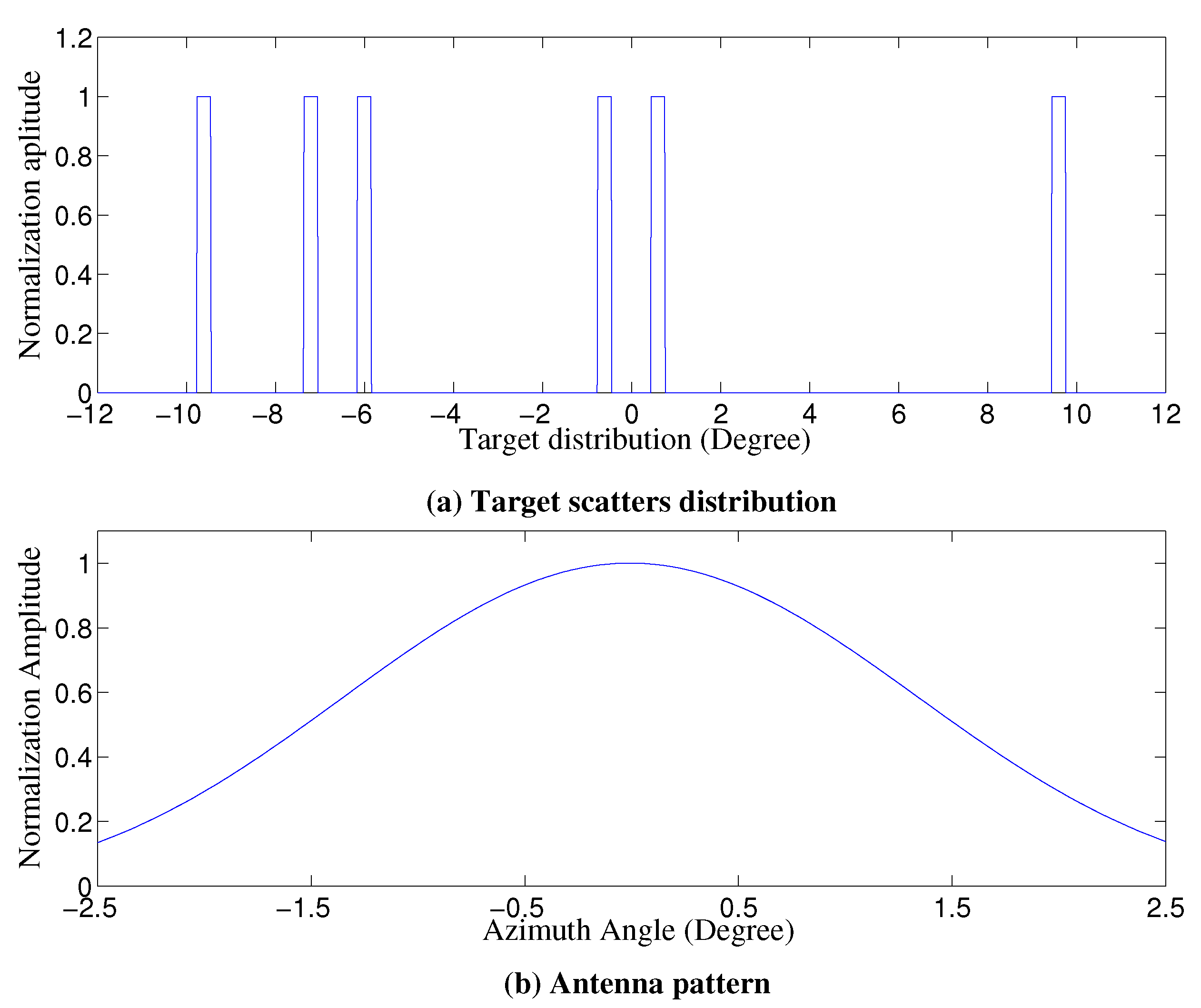
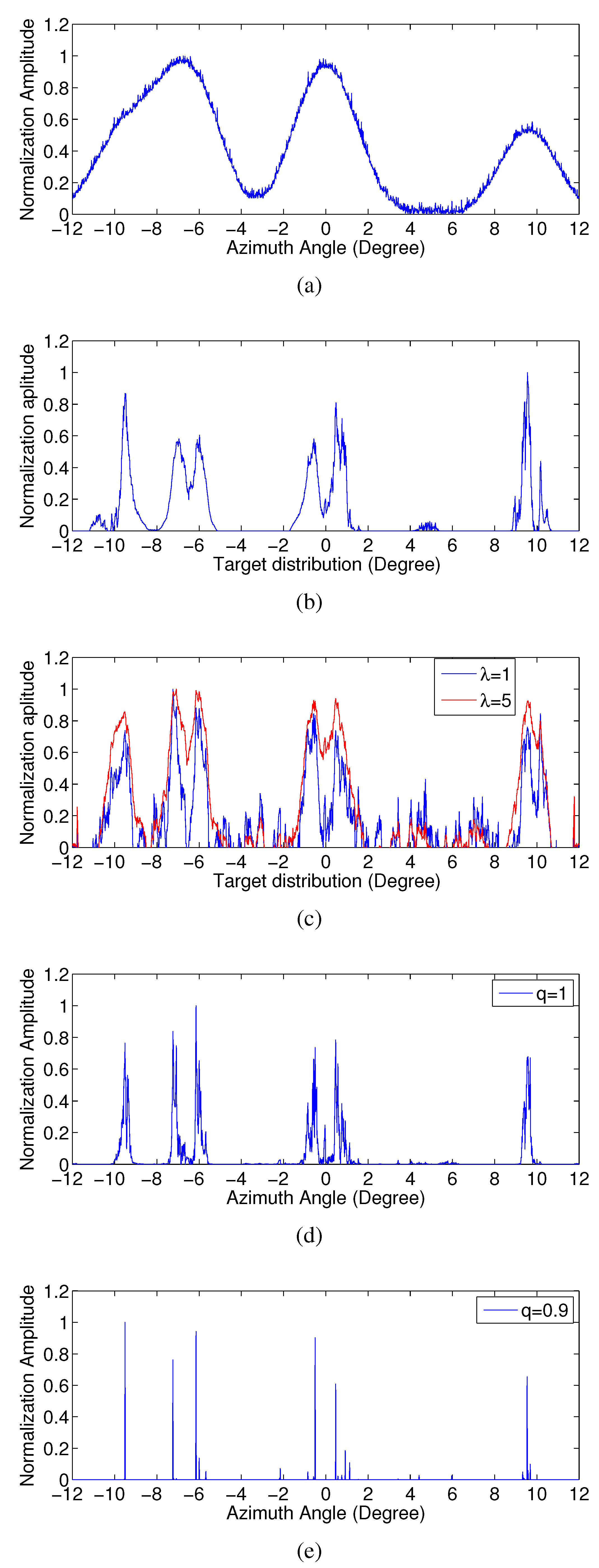
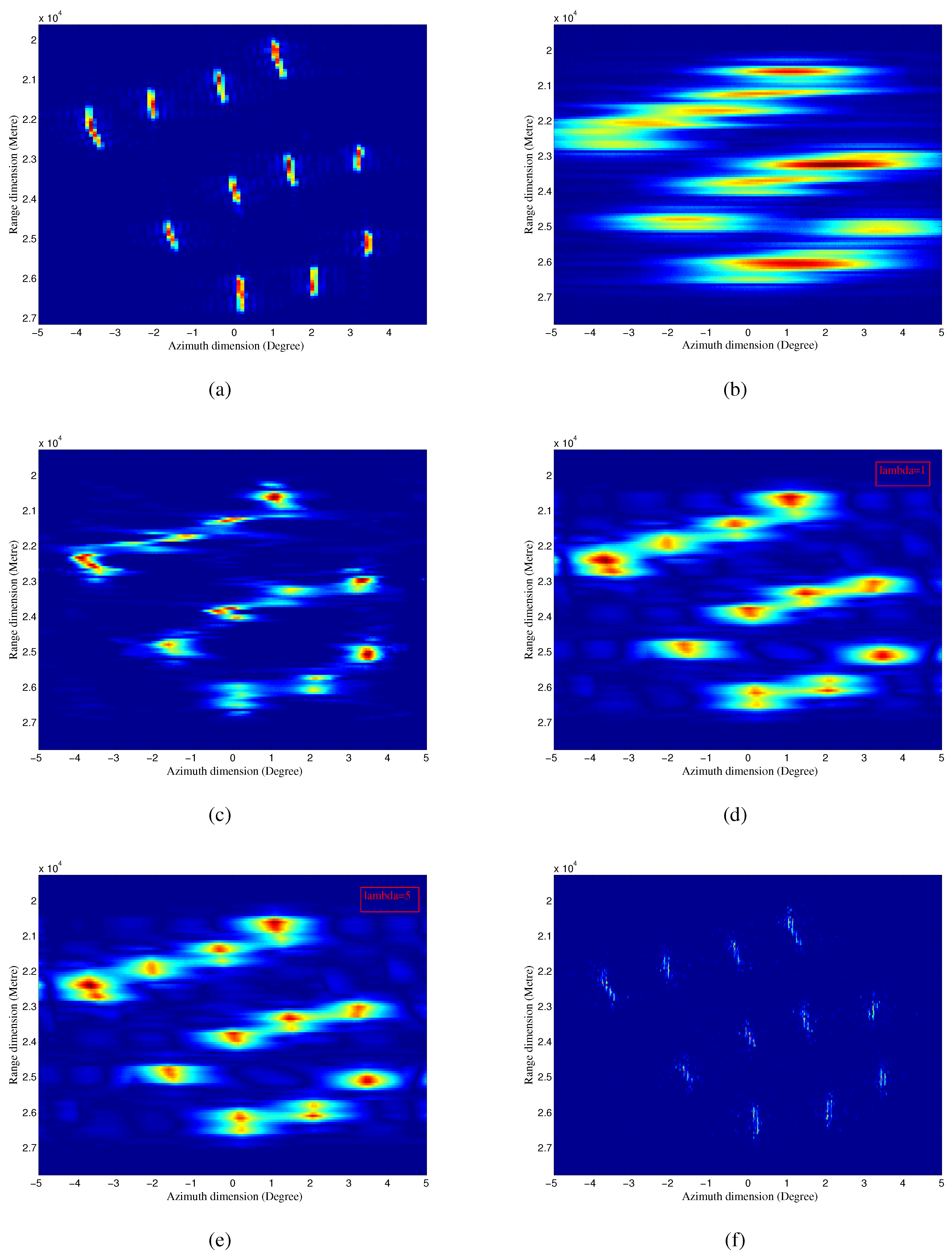
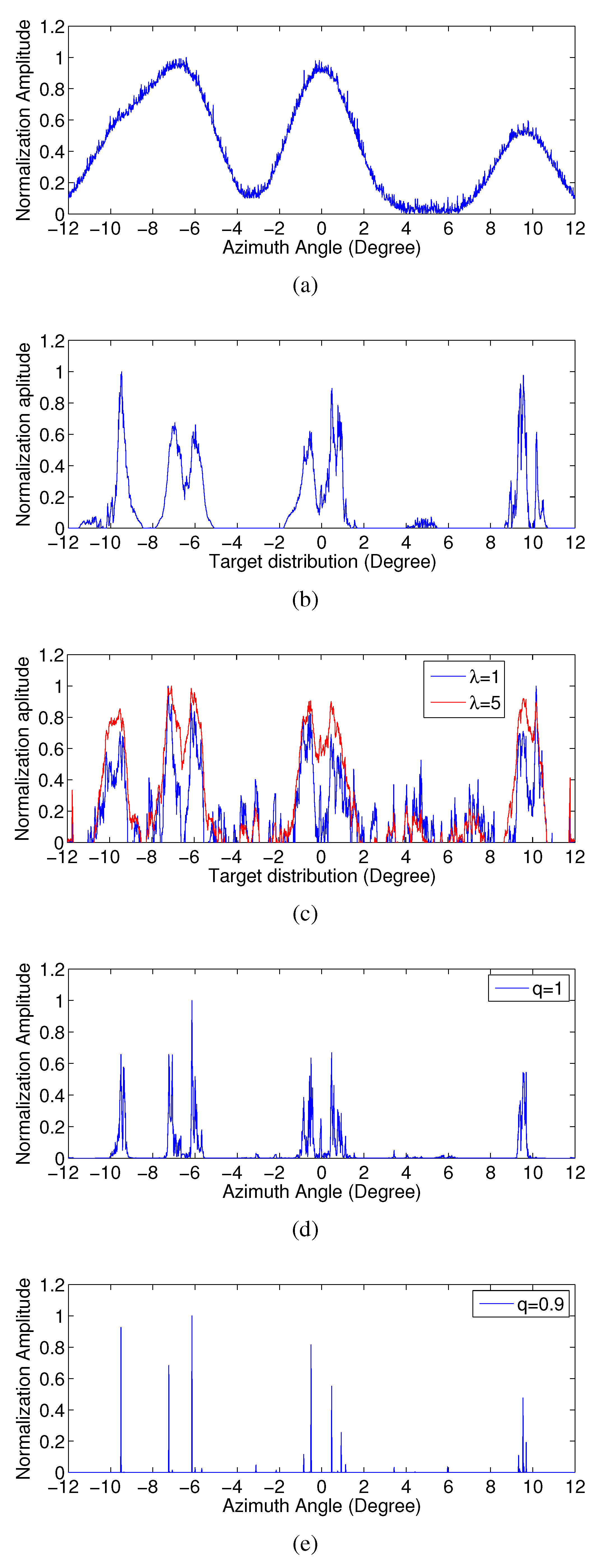
4.1. Point Target Simulation

Figure 2 shows the target distribution and antenna pattern. In Figure 2a, three groups of extended targets with the same amplitude are distributed in the scanning imaging area. The width of the point targets is about 0.3°. Figure 2b shows the antenna pattern which the 3 dB width is 3°. Other important simulation parameters are given in Table 1. Figure 3 and Figure 4 are the simulation results in different SCR conditions. The SCR is defined as:

$$SCR=20{log}_{10}\frac{{∥\mathbf{f}∥}_2}{{∥\mathbf{s}-\mathbf{Hf}∥}_2}$$

(26)

Figure 2. Extended point targets distribution and antenna pattern.

Figure 2. Extended point targets distribution and antenna pattern.

Table 1. Simulation parameters.

Parameter	Value	Units
Carrier frequency	9.6	GHz
Band width	30	MHz
Antenna scanning velocity	30	°/s
Antenna scanning area	$-12\sim +12$	°
Pulse repetition frequency	2000	Hz
Working distance	10	km

Table 1. Simulation parameters.

Parameter	Value	Units
Carrier frequency	9.6	GHz
Band width	30	MHz
Antenna scanning velocity	30	°/s
Antenna scanning area	$-12\sim +12$	°
Pulse repetition frequency	2000	Hz
Working distance	10	km

The SCR is 25 dB in the simulations of Figure 3. Figure 3a shows the real aperture signal, which had very low azimuth angular resolution. We cannot estimate the number and position of these targets. Figure 3b–e shows the superresolution results processed by different algorithms. In the simulations, the Tikhonov regularization algorithm had limited superresolution performance. The red and blue lines were the superresolution results when the regularization parameter λ was set to five and one, respectively. This algorithm also faced a trade-off between the image quality and resolution. High resolution was at the cost of noise amplification. Compared to the Tikhonov regularization algorithm, the RL algorithm had better superresolution performance. This algorithm sharpened the isolated target and improved the resolution, but this algorithm cannot totally distinguish the adjacent targets. In general, our algorithm achieved the best angular superresolution performance. Different values of q both realized a high resolution. Even if some false targets with a small amplitude appeared in the simulation results, it has a small effect for practical application. However, we need to make a trade-off between the resolution and contour features of the image. We can select a small value of q for a higher resolution or we can consider $q\to 1$ for better contour features. We need to choose a suitable value of q according to the practical requirement.

Figure 4 shows the simulation results when the SCR is 20 dB. Obviously, the RL algorithm and Tikhonov regularization had performance degradation with the decrease of SCR. In the simulation results of the two algorithms, some false targets with strong normalization amplitudes appeared. In Figure 4b, the isolated target at $9.5$° became two targets. This phenomenon became much worse in the simulation results of Tikhonov regularization. The noise amplified to an unacceptable level when $\lambda =1$. In the simulation results of the proposed algorithm, the performance degradation is under an acceptable level. The proposed algorithm still sharpened the isolated target and distinguished the adjacent targets.

Figure 3. Simulation results of extended point targets when the signal-to-clutter ratio (SCR) is 25 dB. (a) Real aperture signal. (b) Richardson-Lucy (RL) algorithm. (c) Tikhonov regularization with different regularization parameters. (d) Proposed algorithm when $q=1$. (e) Proposed algorithm when $q=0.9$.

Figure 3. Simulation results of extended point targets when the signal-to-clutter ratio (SCR) is 25 dB. (a) Real aperture signal. (b) Richardson-Lucy (RL) algorithm. (c) Tikhonov regularization with different regularization parameters. (d) Proposed algorithm when $q=1$. (e) Proposed algorithm when $q=0.9$.

Figure 4. Simulation results of extended point targets when the SCR is 20 dB. (a) Real aperture signal. (b) RL algorithm. (c) Tikhonov regularization with different regularization parameters. (d) Proposed algorithm when $q=1$. (e) Proposed algorithm when $q=0.9$.

Figure 4. Simulation results of extended point targets when the SCR is 20 dB. (a) Real aperture signal. (b) RL algorithm. (c) Tikhonov regularization with different regularization parameters. (d) Proposed algorithm when $q=1$. (e) Proposed algorithm when $q=0.9$.

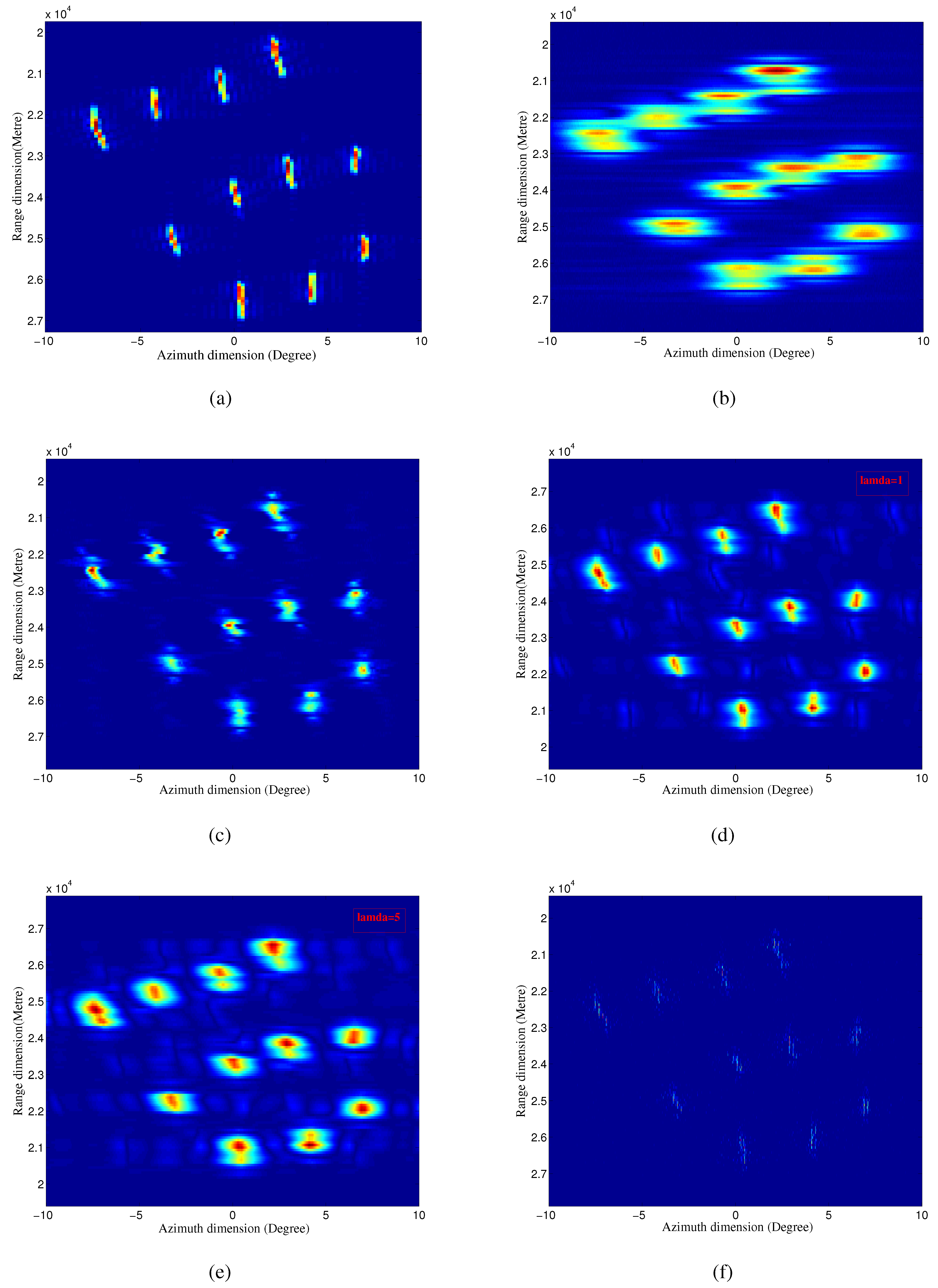
4.2. Scene Simulation

Figure 5 and Figure 6 show the simulation results of the same scene, which are distributed in different scanning imaging regions. We select $q=0.95$ in the two group of simulations, because this parameter made a good balance between the resolution and contour features of the image. The SCR in the two group simulations are both 20 dB, and the working distance is 20 km. In Figure 5, the scene was distributed in the $-10$° to 10° area. Figure 5c–f shows that all of these techniques successfully improved the azimuth angular resolution, because the angular interval of adjacent targets was similar to the real aperture width. However, some targets were distorted in the simulation result of the RL algorithm. Besides, in the simulation results of Tikhonov regularization, the spots that were caused by the noise amplification influenced the image quality to a certain extent. The proposed algorithm exhibited the best superresolution capability. After the processing of the proposed MAP algorithm, the width of recovered point targets was almost equal to the original targets. Besides, the loss of the scattering coefficient had a small effect on the practical application.

In Figure 6, the scene was distributed in the $-5$° to 5° area. The angular interval of different targets was about half of the real aperture width, which caused the overlap of the received echo. We can clearly find the performance degradation in the simulation results of the RL algorithm and Tikhonov regularization. In Figure 6c, the phenomenon of target distortion seriously influenced the estimation the target number and position. In Figure 6d,e, most of the targets cannot be resolved, and noise amplification still impacted the image quality. In Figure 6f, we can find that the proposed MAP algorithm still had high performance. The resolution was improved, and the noise was suppressed. The simulation results of the scene could verify the effectiveness of our proposed algorithm.

Figure 5. Simulation results of the scene when the imaging region is from $-10$° to 10°. (a) Original scene. (b) Real aperture image. (c) RL algorithm. (d) Tikhonov regularization when $\lambda =1$. (e) Tikhonov regularization when $\lambda =5$. (f) Proposed MAP algorithm when $q=0.95$.

Figure 5. Simulation results of the scene when the imaging region is from $-10$° to 10°. (a) Original scene. (b) Real aperture image. (c) RL algorithm. (d) Tikhonov regularization when $\lambda =1$. (e) Tikhonov regularization when $\lambda =5$. (f) Proposed MAP algorithm when $q=0.95$.

Figure 6. Simulation results of the scene when the imaging region is from $-5$° to 5°. (a) Original scene. (b) Real aperture image. (c) RL algorithm. (d) Tikhonov regularization when $\lambda =1$. (e) Tikhonov regularization when $\lambda =5$. (f) Proposed MAP algorithm when $q=0.95$.

Figure 6. Simulation results of the scene when the imaging region is from $-5$° to 5°. (a) Original scene. (b) Real aperture image. (c) RL algorithm. (d) Tikhonov regularization when $\lambda =1$. (e) Tikhonov regularization when $\lambda =5$. (f) Proposed MAP algorithm when $q=0.95$.

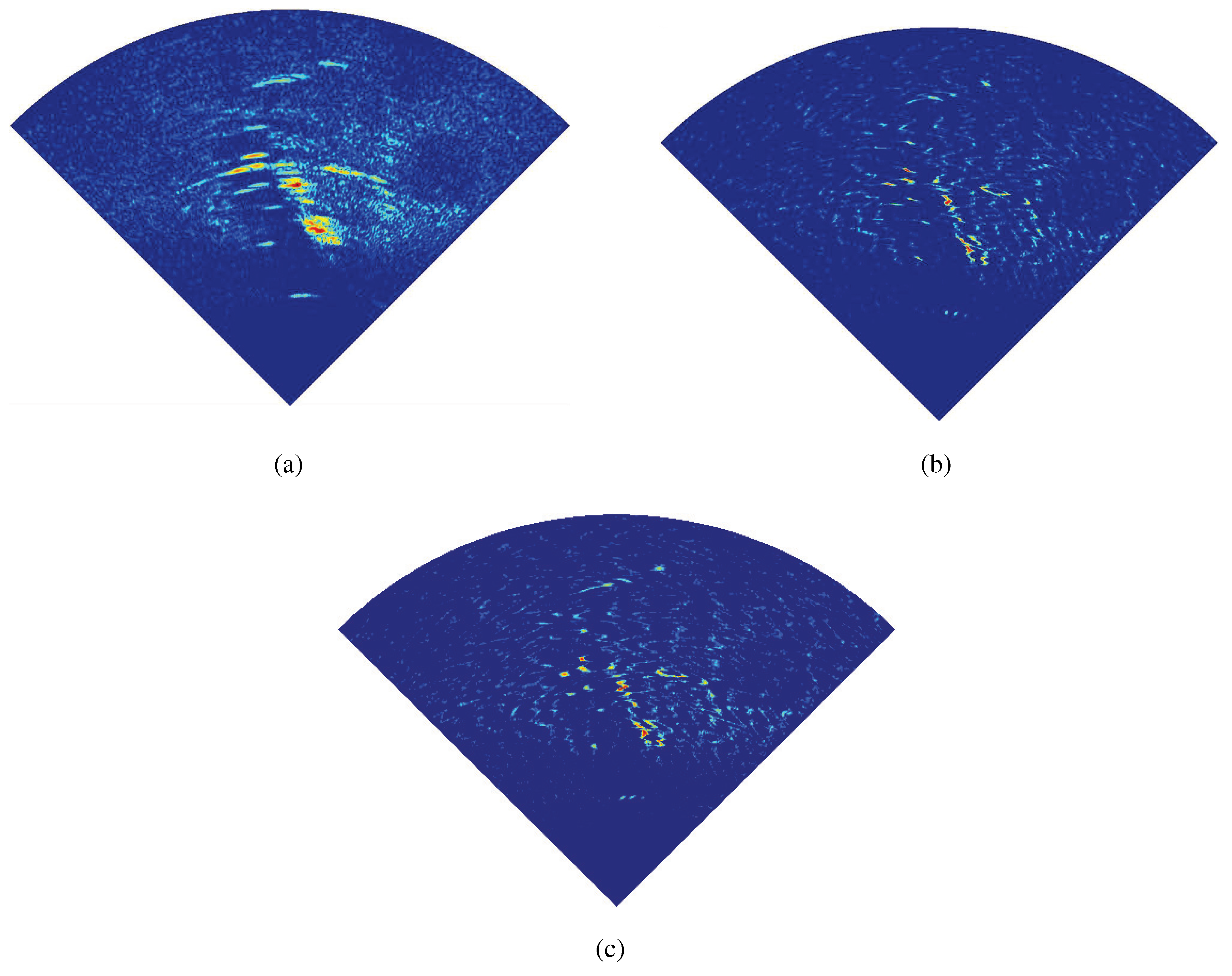
4.3. Real Measured Data

The performance of the new method can also be proven by real measured data. Here, the measured X band radar data were employed to verify the performance of the proposed MAP algorithm.

Figure 7 is the measured data from a far distance scene, which was recorded by a real aperture scanning radar. Figure 7a shows that the real aperture image had limited azimuth resolution after the operation of pulse compression. Figure 7b,c shows the superresolution results of the RL algorithm and the proposed MAP algorithm, respectively. We selected $q=0.95$ in the simulation of the proposed algorithm. By testing the target width before and after the processing of the proposed and the RL algorithm, we can find that the proposed algorithm improved the resolution of the strong scattering target about four times. The RL algorithm only improved the angular resolution about two times. The measured data also demonstrate that the proposed algorithm is an effective method for the real aperture imaging.

Figure 7. Superresolution results of the measured data processed by the RL algorithm and the proposed MAP algorithm. (a) Measured real aperture image. (b) RL algorithm. (c) Proposed MAP algorithm.

Figure 7. Superresolution results of the measured data processed by the RL algorithm and the proposed MAP algorithm. (a) Measured real aperture image. (b) RL algorithm. (c) Proposed MAP algorithm.

5. Conclusions

The azimuth angular superresolution problem has received much attention in recent years, but little work on the angular superresolution of a real aperture scanning radar has been reported. This radar system has wide potential applications, such as the superresolution of a stationary platform and the forward-looking region of a motion platform. The deconvolution method based on the MAP criterion was proposed to deal with the low azimuth resolution problem, because the azimuth dimension of the real aperture scanning radar can be regarded as the convolution of the target scattering coefficient and antenna pattern.

For high superresolution precision in clutter background, the common clutter property and target distribution were considered in the proposed MAP algorithm. Simulations and real measured data show that the proposed method can effectively improve the azimuth resolution and reduce the interference of clutter. This approach could be widely applied in the detection and tracking of a strong scattering target. Besides, this approach also could be applied to the Direction Of Arrival estimation of array signal processing.

References

1. Skolnik, M.I. Introduction to radar. Radar Handb. 1962, 2. Available online: http://www.turma-aguia.com/davi/skolnik/Skolnik_chapter_1.pdf (accessed on 10 October 2015). [Google Scholar]
2. Wehner, D.R. High Resolution Radar; Artech House: Norwood, MA, USA, 1987; p. 484. [Google Scholar]
3. Senmoto, S.; Childers, D. Signal resolution via digital inverse filtering. IEEE Trans. Aerosp. Electron. Syst. 1972, 5, 633–640. [Google Scholar] [CrossRef]
4. Richards, M.A. Iterative noncoherent angular superresolution [radar]. In Proceedings of the 1988 IEEE National Radar Conference, Ann Arbor, MI, USA, 20–21 April 1988.
5. Migliaccio, M.; Gambardella, A. Microwave radiometer spatial resolution enhancement. IEEE Trans. Geosci. Remote Sens. 2005, 43, 1159–1169. [Google Scholar] [CrossRef]
6. Gambardella, A.; Migliaccio, M. On the superresolution of microwave scanning radiometer measurements. IEEE Geosci. Remote Sens. Lett. 2008, 5, 796–800. [Google Scholar] [CrossRef]
7. Bose, R.; Freedman, A.; Steinberg, B.D. Sequence CLEAN: A modified deconvolution technique for microwave images of contiguous targets. IEEE Trans. Aerosp. Electron. Syst. 2002, 38, 89–97. [Google Scholar] [CrossRef]
8. Pérez-Martínez, F.; García-Fominaya, J.; Calvo-Gallego, J. A shift-and-convolution technique for high-resolution radar images. IEEE Sens. J. 2005, 5, 1090–1098. [Google Scholar] [CrossRef]
9. Ly, C.; Dropkin, H.; Manitius, A.Z. Extension of the MUSIC algorithm to millimeter-wave (MMW) real-beam radar scanning antennas. In Proceedings of Radar Sensor Technology and Data Visualization, Orlando, FL, USA, 1 April 2002.
10. Uttam, S.; Goodman, N.A. Superresolution of Coherent Sources in Real-Beam Data. IEEE Trans. Aerosp. Electron. Syst. 2010, 46, 1557–1566. [Google Scholar] [CrossRef]
11. Yardibi, T.; Li, J.; Stoica, P.; Xue, M.; Baggeroer, A.B. Source localization and sensing: A nonparametric iterative adaptive approach based on weighted least squares. IEEE Trans. Aerosp. Electron. Syst. 2010, 46, 425–443. [Google Scholar] [CrossRef]
12. Roberts, W.; Stoica, P.; Li, J.; Yardibi, T.; Sadjadi, F.A. Iterative adaptive approaches to MIMO radar imaging. IEEE J. Sel. Top. Signal Process. 2010, 4, 5–20. [Google Scholar] [CrossRef]
13. Stoica, P.; Li, J.; Ling, J. Missing data recovery via a nonparametric iterative adaptive approach. IEEE Signal Process. Lett. 2009, 16, 241–244. [Google Scholar] [CrossRef]
14. Zhang, Y.; Zhang, Y.; Li, W.; Huang, Y.; Yang, J. Angular superresolution for real beam radar with iterative adaptive approach. In Proceedings of 2013 IEEE International Geoscience and Remote Sensing Symposium (IGARSS), Melbourne, Austrilia, 21–26 July 2013.
15. Zhang, Y.; Zhang, Y.; Huang, Y.; Yang, J.; Zha, Y.; Wu, J.; Yang, H. ML iterative superresolution approach for real-beam radar. In Proceedings of 2014 IEEE Radar Conference, Cincinnati, OH, USA, 19–23 May 2014.
16. Lenti, F.; Nunziata, F.; Migliaccio, M.; Rodriguez, G. Two-Dimensional TSVD to enhance the spatial resolution of radiometer data. IEEE Trans. Geosci. Remote Sens. 2014, 52, 2450–2458. [Google Scholar] [CrossRef]
17. Lenti, F.; Nunziata, F.; Estatico, C.; Migliaccio, M. On the spatial resolution enhancement of microwave radiometer data in Banach spaces. IEEE Trans. Geosci. Remote Sens. 2014, 52, 1834–1842. [Google Scholar] [CrossRef]
18. Schiavulli, D.; Nunziata, F.; Pugliano, G.; Migliaccio, M. Reconstruction of the normalized radar cross section field from GNSS-R delay-Doppler map. IEEE J. Sel. Top. Appl. Earth Obs. Remote Sens. 2014, 7, 1573–1583. [Google Scholar] [CrossRef]
19. Schiavulli, D.; Lenti, F.; Nunziata, F.; Pugliano, G.; Migliaccio, M. Landweber method in Hilbert and Banach spaces to reconstruct the NRCS field from GNSS-R measurements. Int. J. Remote Sens. 2014, 35, 3782–3796. [Google Scholar] [CrossRef]
20. Tan, X.; Roberts, W.; Li, J.; Stoica, P. Sparse learning via iterative minimization with application to MIMO radar imaging. IEEE Trans. Signal Process. 2011, 59, 1088–1101. [Google Scholar] [CrossRef]
21. Xu, G.; Xing, M.; Zhang, L.; Liu, Y.; Li, Y. Bayesian inverse synthetic aperture radar imaging. IEEE Geosci. and Remote Sens. Lett. 2011, 8, 1150–1154. [Google Scholar] [CrossRef]
22. Zha, Y.; Huang, Y.; Yang, J.; Wu, J.; Zhang, Y.; Yang, H. An improved Richardson-Lucy algorithm for radar angular super-resolution. In Proceedings of 2014 IEEE Radar Conference, Cincinnati, OH, USA, 19–23 May 2014.
23. Golub, G.H.; Hansen, P.C.; O’Leary, D.P. Tikhonov regularization and total least squares. SIAM J. Matrix Anal. Appl. 1999, 21, 185–194. [Google Scholar] [CrossRef]
24. Boyd, S.; Vandenberghe, L. Convex Optimization; Cambridge University Press: Cambridge, UK, 2004. [Google Scholar]
25. Chartrand, R. Exact reconstruction of sparse signals via nonconvex minimization. IEEE Signal Process. Lett. 2007, 14, 707–710. [Google Scholar] [CrossRef]
26. Vu, D.; Xue, M.; Tan, X.; Li, J. A Bayesian approach to SAR imaging. Digit. Signal Process. 2013, 23, 852–858. [Google Scholar] [CrossRef]
27. Kuruoglu, E.E.; Zerubia, J. Modeling SAR images with a generalization of the Rayleigh distribution. IEEE Trans. Image Process. 2004, 13, 527–533. [Google Scholar] [CrossRef] [PubMed]
28. Anastassopoulos, V.; Lampropoulos, G.A.; Drosopoulos, A.; Rey, M. High resolution radar clutter statistics. IEEE Trans. Aerosp. Electron. Syst. 1999, 35, 43–60. [Google Scholar] [CrossRef]
29. Migliaccio, M.; Ferrara, G.; Gambardella, A.; Nunziata, F.; Sorrentino, A. A physically consistent speckle model for marine SLC SAR images. IEEE J. Ocean. Eng. 2007, 32, 839–847. [Google Scholar] [CrossRef]
30. Snyder, D.L.; Helstrom, C.W.; Lanterman, A.D.; Faisal, M.; White, R.L. Compensation for readout noise in CCD images. J. Opt. Soc. Am. A 1995, 12, 272–283. [Google Scholar] [CrossRef]
31. Dey, N.; Blanc-Feraud, L.; Zimmer, C.; Roux, P.; Kam, Z.; Olivo-Marin, J.C.; Zerubia, J. Richardson-Lucy algorithm with total variation regularization for 3D confocal microscope deconvolution. Microsc. Res. Tech. 2006, 69, 260–266. [Google Scholar] [CrossRef] [PubMed]
32. Ward, K.D.; Watts, S.; Tough, R.J. Sea Clutter: Scattering, the K Distribution and Radar Performance; IET: Stevenage, UK, 2006. [Google Scholar]
33. Oliver, C.; Quegan, S. Understanding Synthetic Aperture Radar Images; SciTech Publishing: Stevenage, UK, 2004. [Google Scholar]
34. Dey, S.; Dey, T.; Kundu, D. Two-Parameter Rayleigh Distribution: Different Methods of Estimation. Am. J. Math. Manag. Sci. 2014, 33, 55–74. [Google Scholar] [CrossRef]