A Potential Flow Theory and Boundary Layer Theory Based Hybrid Method for Waterjet Propulsion

Abstract

A hybrid method—coupled with the boundary element method (BEM) for wave-making resistance, the empirical method (EM) for viscous resistance, and the boundary layer theory (BLT) for capture of an area’s physical parameters—was proposed to predict waterjet propulsion performance. The waterjet propulsion iteration process was established from the force-balanced waterjet–hull system by applying the hybrid approach. Numerical validation of the present method was carried out using the 1/8.556 scale waterjet-propelled ITTC (International Towing Tank Conference) Athena ship model. Resistance, attitudes, wave cut profiles, waterjet thrust, and thrust deduction showed similar tendencies to the experimental curves and were in good agreement with the data. The application of the present hybrid method to the side-hull configuration research of a trimaran indicates that the side-hull arranged at the rear of the main hull contributed to energy-saving and high-efficiency propulsion. In addition, at high Froude numbers, the “fore-body trimaran” showed a local advantage in resistance and thrust deduction.

1. Introduction

The prediction of the waterjet thrust and thrust deduction is an important part of the hydrodynamic performance of the waterjet propulsion system. There are mainly three kinds of prediction methods: the theoretical analysis method, the model test method, and the CFD (computational fluid dynamics) method. The first method is based on experimental statistic data. The equilibrium equation composed of the Bernoulli equation and the energy loss equation determined by empirical coefficients was established to solve the equation of thrust. The model test method was proposed by the ITTC (International Towing Tank Conference). Thrust was obtained by direct measurement or by using the momentum flux method with a measured velocity field at both the inlet and the jet. The CFD method based on the momentum flux theory has been widely applied to obtain waterjet propulsion performance in recent years.

The research on waterjet propulsion carried out in the 1990s concentrates on waterjet–hull interaction [1,2,3,4]. The standardization of waterjet thrust prediction and measurement, which was proposed by the Specialist Committee on Waterjets of the ITTC [5], greatly contributes to the development of the CFD method in the waterjet propulsion field. The intake duct system was researched based on the viscous CFD method [6,7,8,9,10]. This research focuses on the ducting system itself without considering the influence of the ship due to the limitation of computer hardware. Later, the rapid development of the computer provided the basis for a large-scale parallel CFD numerical simulation. Takai et al. [11,12] completed a multi-objective optimization of a ship with the waterjet propulsion system. The research of Altosole et al. [13] provides a reliable and effective method to optimize the parameters of the waterjet propulsion system for a high-speed vessel. Eslamdoost [14,15] used the potential flow module XPAN and the double model module XBOUND to study the waterjet–hull interaction problem based on the pressure jump method.

The numerical research of hydrodynamics of marine structures mainly adopts the potential flow CFD [16,17] and the viscous flow CFD method [18], which captures more details of the flow field. However, the computational efficiency of viscous flow CFD still needs to be improved, and a rapid thrust prediction method is required in the preliminary design stage for the waterjet ship. In this present study, the potential flow theory and boundary layer theory-based hybrid method is proposed to rapidly and efficiently achieve the calculation of waterjet propulsion performance. The validation process was also carried out.

2. Theory

2.1. The Force-Balanced Waterjet–Hull System

The waterjet–hull system consists of two parts: the waterjet system and the rest hull surface. In the waterjet duct, the fluid pressure and velocity of the fluid change is greatly due to the rotation of the pump rotor. In this study, the rotor and stator are assumed to be a virtual disk, and the pressure jump occurs when the fluid passes the virtual disk [14]. The longitudinal force of the hull motion resistance is considered as follows (details of the symbols are listed at the end of the article):

$$R_{p,x}=R_H+N\cdot R_{D,x}+N\cdot R_{N,x}$$

(1)

where N is the number of waterjet sets (waterjets units are assumed to be the same), R_H is the total resistance of the hull (excluding the duct), R_D,x is the longitudinal force of each duct before the pump, and R_N,x is the longitudinal force of each nozzle chamber after the pump.

The pressure before and after the pump (virtual disk) is P_b and P_a, respectively, and the section area of duct at rotor is A_i. There is a balance between the resultant force of the hull and the thrust of the waterjet system while taking the trim angle θ into account:

$$R_{p,x}=F_x=N{A}_i(P_a-P_b)\cos \theta =N\Delta p{A}_i\cos \theta$$

(2)

The longitudinal force of the duct in waterjet propulsion can be calculated by using the following equation:

$$R_{N,x}=N{\displaystyle \underset{S_n}{\iint }{\sigma }_t\cdot n_{x}ds}=N{\displaystyle \underset{S_n}{\iint }(p+\tau )n_{x}ds}$$

(3)

where S_n is the inner surface of the nozzle chamber.

The flow passing through the pump area gets an acceleration in velocity due to the pressure jump. The pressure after the virtual disk can separate to a constant flow pressure, P_c, and the pressure difference $\Delta p$:

$${\displaystyle \underset{S_n}{\iint }p\cdot n_{x}ds}={\displaystyle \underset{S_n}{\iint }{p}_c\cdot n_{x}ds+}{\displaystyle \underset{S_n}{\iint }\Delta p\cdot n_{x}ds}$$

(4)

Inside the nozzle chamber:

$${\displaystyle \underset{S_n}{\iint }\Delta p\cdot n_{x}ds}=\Delta p(A_i-A_n)\cos \theta$$

(5)

From Equations (1)–(5), we obtained:

$$N\Delta p\cdot A_n\cos \theta =R_H+N{R}_{D,x}+N\left({\displaystyle \underset{S_n}{\iint }{p}_c\cdot n_{x}ds+{\displaystyle \underset{S_n}{\iint }\tau \cdot n_{x}ds}}\right)$$

(6)

Equation (6) is the sum of forces except the pressure jump at the virtual disk in the whole system:

$$R_{RT}=R_H+N{R}_{D,x}+N\left({\displaystyle \underset{S_n}{\iint }{p}_c\cdot n_{x}ds+{\displaystyle \underset{S_n}{\iint }\tau \cdot n_{x}ds}}\right)$$

(7)

Then, the expression of the pressure jump is obtained using the equation: $\Delta p=\frac{R_{RT}}{N{A}_n\cos \theta }$.

2.2. Iterative Solution Model

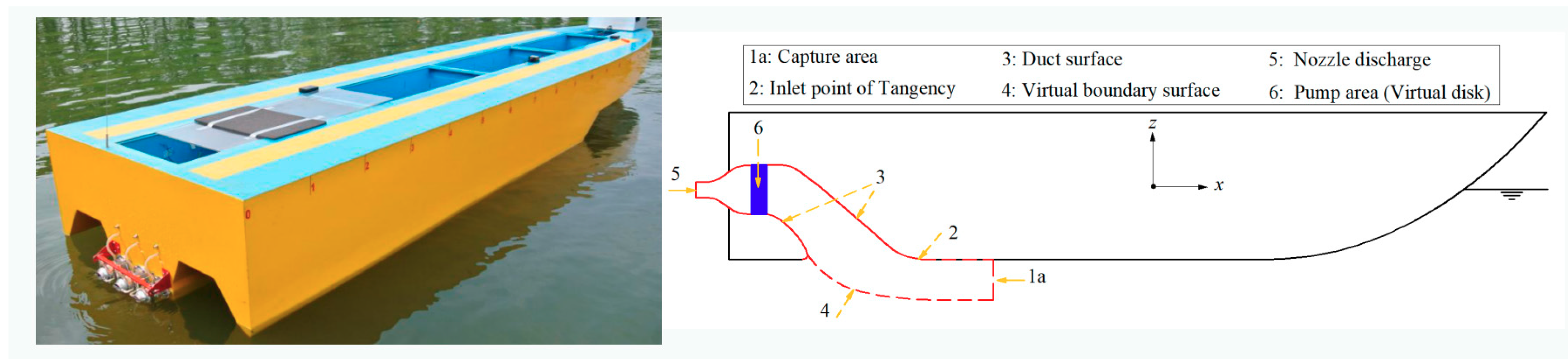
The thrust of the waterjet propulsion was solved in a virtual control volume based on the momentum flux method [19]. A closed control volume consists of the capture area (1a), the duct surface (3), the virtual boundary surface (4), and the nozzle discharge (5), as shown in Figure 1.

Considering the local losses caused by frictional retardation, flow direction changes in the duct, duct expansion, and contraction, the pressure head balance applied in the center of the capture area and the nozzle discharge, there is:

$$\left({\overline{p}}_{1a}+\rho g{\overline{h}}_{1a}+\frac{1}{2}\rho \overline{u_{1a}^2}\right)+\Delta p={\overline{p}}_5+\rho g{\overline{h}}_5+\frac{1}{2}\rho \overline{u_5^2}+K\frac{1}{2}\rho \overline{u_0^2}$$

(8)

The nozzle velocity ratio was obtained using the following equation:

$$NVR=\frac{\overline{u_5}}{u_0}=\sqrt{\frac{2({\overline{p}}_{1a}-{\overline{p}}_5)}{\rho u_0^2}+\frac{2\Delta p}{\rho u_0^2}+\frac{2g({\overline{h}}_{1a}-{\overline{h}}_5)}{u_0^2}+IV{R}^2-K}$$

(9)

where $u_0$ is the advance velocity of the ship, $IVR=\overline{u_{1a}}/u_0$ is the inlet velocity ratio, $\overline{u_{1a}}$ and $\overline{u_5}$, $\overline{p_{1a}}$ and $\overline{p_5}$, and $\overline{h_{1a}}$ and $\overline{h_5}$ represent the average velocity, average pressure, and average height above the baseline of the capture area and nozzle respectively. K is the local loss coefficient of the duct, including friction loss, flow direction loss, and duct contraction loss. Xia provides more details in his book [20] about the local loss coefficient.

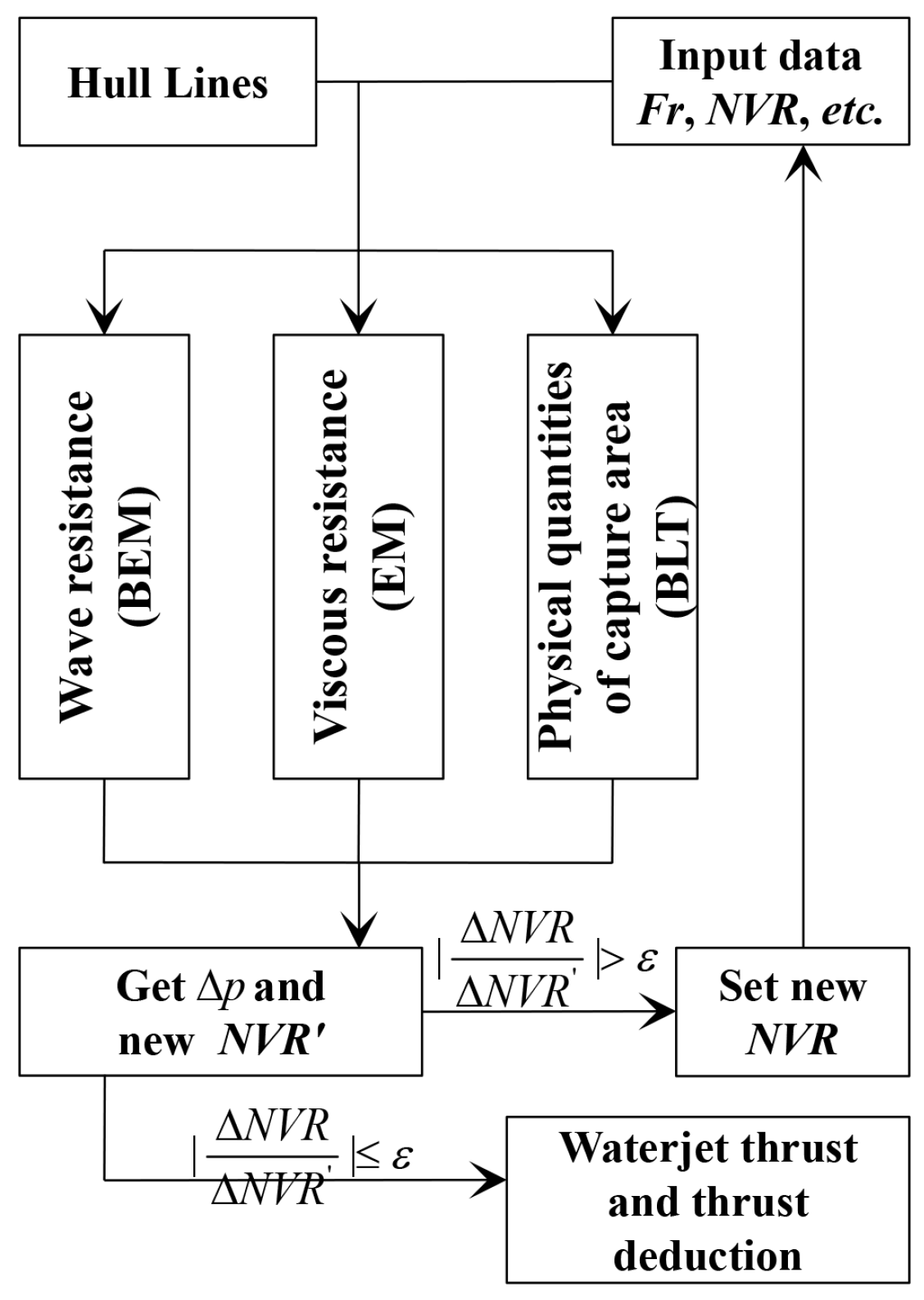
NVR was set as the initial input value in the calculation and a new velocity ratio $NV{R}^{\text{'}}$ can be obtained by using Equation (9), once the force acting on ship and the pressure jump $\Delta p$ are solved. Therefore, the size correlation between the ratio $\left|\Delta NVR\right|/NVR$ and the residual $\epsilon$ we set was the criterion used to determine whether the stop criterion was reached. This concept is illustrated in Figure 2. The waterjet thrust could be computed once the stop criterion was reached.

3. Numerical Method

3.1. Wave-Making Resistance

Based on the basic assumption of the potential flow theory, the fluid is in-viscid, in-compressible, and ideal. The total velocity potential without considering the unsteady disturbances is written as:

$$\Phi (x,y,z)=-u_{0}x+\phi (x,y,z)$$

(10)

where $-u_{0}x$ represents the velocity potential of uniform flow, and $\phi$ is the perturbation velocity potential caused by the uniform velocity motion of the ship, there is:

$${\nabla }^2\phi =0$$

(11)

The free surface boundary condition is:

$$\frac{{\partial }^2\phi }{\partial x^2}+\frac{g}{u_0^2}\frac{\partial \phi }{\partial z}=0$$

(12)

The hull boundary conditions should be specially treated. An additional boundary condition for the nozzle discharge was added to the waterjet propulsion calculation. The hull and duct surface, except the nozzle discharge, were similar to the wall without penetration. The nozzle discharge was set as the velocity boundary with a fixed velocity of $NVR\cdot u_0$. The two boundary conditions were defined as follows:

$$\{\begin{array}{cc}\frac{\partial \phi }{\partial n}=u_0\cdot n_x\hfill & \hfill \left(Hullexceptnozzledischarge\right)\hfill \\ \frac{\partial \phi }{\partial n}=NVR\cdot u_0\cdot n_x\hfill & \hfill \left(Thenozzledischarge\right)\hfill \end{array}$$

(13)

The infinite boundary condition and transom boundary condition [21] were written as:

$$\{\begin{array}{l}\phi \to 0\left(Atinfinity\right)\\ {\phi }_{xx}-2{\phi }_x/\Delta x=-\frac{g}{u_0}(2h_T(x_T-y_T)/\Delta x+\frac{\partial h_T}{\partial x}(x_T-y_T))(Transom)\end{array}$$

(14)

where n_x is the outward normal component of the ship hull surface in the x direction and NVR is the nozzle velocity ratio. In the transom condition, h_T is the height of the transom stern edge. x_T and y_T are the longitudinal and transverse coordinates of the transom stern, respectively. $\Delta x$ is a the finite distance on the free surface after the transom stern, which can be evaluated as half the longitudinal scale of the panel.

The Rankine source panel method [22,23,24] was used to obtain the perturbation potential in the flow field using the discretization of the above equations. The Rankine source Green function can be expressed as $G(p,q)=\frac{1}{r(p,q)}$, where p(x, y, z) is the field point and q(x′, y′, z′) is the source point. Then, the potential velocity at p can be denoted as:

$$\Phi (p)={\displaystyle \sum _{i=1}^N{\displaystyle \underset{S_i}{\iint }\frac{\sigma (q_i)}{4\pi r(p,q_i)}}}d{S}_i$$

(15)

where r(p, q) is the distance between p and q. The total number of panels (N_t) can be divided into the panels of the hull (N_s), panels of the nozzle discharge (N_z), and panels of the free surface (N_f). This can be represented as N_t = N_s + N_z + N_f. S_i indicating the number i panels. Applying Equations (13)–(15), we can obtain the discrete hull surface boundary equation:

$$-\frac{1}{2}\sigma (p_j)+{\displaystyle \sum _{i=1,j\ne i}^N\sigma (q_i)}{\displaystyle \underset{S}{\iint }\frac{\partial }{\partial n}(\frac{1}{4\pi r(p_j,q_i)})}dS=\{\begin{array}{ll}{u}_0\cdot n_x(p_j)& (j=1,2,\cdot \cdot \cdot ,N_s)\\ NVR\cdot u_0\cdot n_x(p_j)& (j=N_s+1,\cdot \cdot \cdot ,N_s+N_z)\end{array}$$

(16)

Free surface and transom boundary condition are converted to the new discrete form:

$${\displaystyle \sum _{i=1,j\ne i}^N\sigma (q_i)}{\displaystyle \underset{S}{\iint }(\frac{{\partial }^2}{\partial x^2}+\frac{g}{u_0^2}\frac{\partial }{\partial z})(\frac{1}{4\pi r(p_j,q_i)})}dS=0(j=N_s+N_z+1,\cdot \cdot \cdot ,N)$$

(17)

$${\displaystyle \sum _{i=1,j\ne i}^N\sigma (q_i)}{\displaystyle \underset{S}{\iint }(\frac{{\partial }^2}{\partial x^2}-\frac{2}{\Delta x}\frac{\partial }{\partial x})(\frac{1}{4\pi r(p_j,q_i)})}dS=-\frac{g}{u_0}(2h_T(x_T-y_T)/\Delta x+\frac{\partial h_T}{\partial x}(x_T-y_T))$$

(18)

To fulfill the infinity radiation condition and avoid the singularity in the integration of the free surface panels, the source points of the free surface panels should manually rise up for 0.5–2.5 $\Delta x$ and the field points should move forward about Δx. By combining the discrete Equations (15)–(18), the source strength could be solved to get the potential velocity.

Then the hull surface pressure distribution was obtained according to the Bernoulli equation:

$$P=\rho \left(u_0\frac{\partial \phi }{\partial x}-\frac{1}{2}\nabla \phi \cdot \nabla \phi -gz\right)$$

(19)

The fluid force in the x directional was obtained by integration of the pressure distribution P, which is the wave-making resistance of the hull:

$$R_w=-F_x={\displaystyle \underset{S}{\iint }P\cdot n_x}dS$$

(20)

The trim and sinkage of the ship were resolved though the force and moment balance equations as follows [25,26]:

$${\displaystyle \underset{S}{\iint }{C}_p{n}_z}ds={\displaystyle {\int }_0^L(s-x\tan \theta )y(x,0)dx}=s{\displaystyle {\int }_0^{L}y(x,0)dx+}\tan \theta {\displaystyle {\int }_0^{L}xy(x,0)dx}$$

(21)

$${\displaystyle \underset{S}{\iint }x{C}_p{n}_z}ds={\displaystyle {\int }_0^L(s-x\tan \theta )xy(x,0)dx}=s{\displaystyle {\int }_0^{L}xy(x,0)dx}+\tan \theta {\displaystyle {\int }_0^L{x}^{2}y(x,0)dx}$$

(22)

where $C_p=P/(0.5\rho u_0^2)$ is the pressure coefficient of the control point on the hull panel, s represents the sinkage, and y(x, 0) is the width of the waterline at x under floating in an even keel state. The initial value of s and $\theta$ was set as 0. The continuous iteration was used to calculate a new s and $\theta$ value along with the mesh being updated until the balance equations converged.

3.2. Viscous Resistance

The 1957ITTC friction resistance coefficient formula was used to calculated the friction resistance of the ship hull:

$$R_f=\frac{1}{2}\rho u_0^2{S}_w\left(\Delta C_f+\frac{0.075}{{(lgRe-2)}^2}\right)$$

(23)

The Reynolds number was defined using the equation $Re=u_0{L}_{wl}/\nu$, where L_wl is the waterline length, $\nu$ is the kinematic viscosity of water, and the roughness allowance is $\Delta C_f=0.4\times {10}^{-3}$ in the process of converting the model-scale results to the full-scale ship.

According to the approximate formula of the viscous-pressure resistance coefficient [27]:

$$C_{pv}=\frac{R_{pv}}{\frac{1}{2}\rho u_0^2{S}_w}=0.09\frac{A_m}{S_w}=\sqrt{\sqrt{A_m/2L_r}}$$

(24)

The ship’s viscous pressure resistance is:

$$R_{pv}=\frac{9\rho u_0^2{A}_m}{200}\sqrt{\sqrt{A_m/2L_r}}$$

(25)

where A_m is the cross section area at midship, and L_r is the run length, which should meet the condition: $L_r\ge 4.08\sqrt{A_m}$.

3.3. Physical Quantities of the Capture Area

The velocity and pressure distribution at the capture area were calculated using the boundary layer theory. The velocity distribution formula in the turbulent boundary layer theory is as follows:

$$\frac{u}{u_0}=\{\begin{array}{ll}{\left(\frac{y}{\delta }\right)}^{1/n}& (y\le \delta )\\ 1& (y>\delta )\end{array}$$

(26)

where y is the vertical distance from the hull, and u is the local velocity. The index n was 7 in the model-scale, and 9 in the full-scale [19]. $\delta$ is the thickness of the boundary layer, which is calculated using the Weighardt formula, $\delta =0.27x{(u_{0}x/\upsilon )}^{-1/6}$, at high Re or the plate flow formula, $\delta =0.37x{(u_{0}x/\upsilon )}^{-1/5}$ [28].

The experiments used to measure the capture area with the series IVR (inlet velocity ratio) ranged from 0.25 to 0.71 in front of the inlet point of the tangency carried out by Roberts [7]. It showed that, for a low IVR of <0.39, the capture area occurs as a concave phenomenon. For higher values (i.e., >0.58), the capture area resembles a semi-elliptical. This agrees with the elliptic capture area phenomenon noticed by Alexander [2].

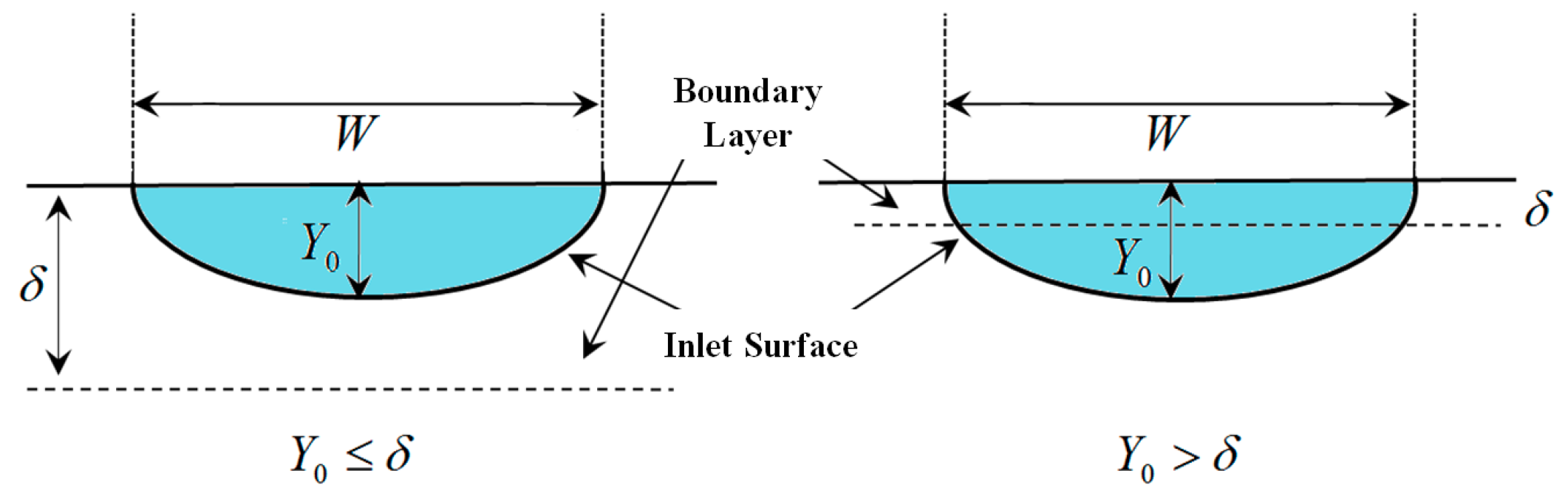
The semi-elliptical shape was used to represent the transverse section of the capture area:

$${(\frac{x}{W/2})}^2+{(\frac{y}{Y_0})}^2=1$$

(27)

where W is the width of capture area recommended to be 50% larger than the geometrical intake width [19]. Y₀ is the effective inflow thickness of the capture area.

There is a basic definition as follows:

$$Q_i={\displaystyle \underset{A_{1a}}{\int }{u}^{i}dA}$$

(28)

where, in the equation i = 1, 2, 3. Q₁, Q₂, and Q₃ represent the inflow volume, inflow momentum, and inflow kinetic energy, respectively. The correlation between the hull boundary layer thickness $\delta$ and Y₀ determined the above parameters and the inlet momentum coefficient.

These parameters were deduced in Liu’s paper [28]. While $Y_0>\delta$, the capture area was divided into two parts, as shown in Figure 3. Liu took the upper part as a rectangle to do the integration. Under this assumption, as the difference between $\delta$ and Y₀ becomes smaller, the numerical error increases. In the present work, the accurate integral formulas were expressed to improve the calculation while $Y_0>\delta$:

$$Q_i={\displaystyle \underset{A_{1a}}{\int }{u}^{i}dA}=u_0^i{Y}_{0}W\left(\frac{\pi }{4}-C_{Qi}^{\text{'}}+\frac{n}{n+i}{(\frac{Y_0}{\delta })}^{i/n}{C}_{Qi}^{″}\right)-\frac{u_0^{i}W\delta }{n+i}{(1-\frac{{\delta }^2}{Y_0^2})}^{1/2}$$

(29)

When $Y_0\le \delta$:

$$Q_i={\displaystyle \underset{A_{1a}}{\int }{u}^{i}dA}=\frac{n}{n+i}{C}_{Qi}{u}_0^i{Y}_{0}W{(\frac{Y_0}{\delta })}^{i/n}$$

(30)

where $C_{Qi}={\displaystyle {\int }_0^1{(1-t^2)}^{\frac{n+i}{2n}}}dt$, $C_{Qi}^{\prime }={\displaystyle {\int }_{\sqrt{1-{\delta }^2/Y_0^2}}^1{(1-t^2)}^{\frac{i}{2}}}dt$, $C_{Qi}^{″}={\displaystyle {\int }_{\sqrt{1-{\delta }^2/Y_0^2}}^1{(1-t^2)}^{\frac{n+i}{2n}}}dt$.

The average velocity of the capture area can be calculated as $\overline{u_{1a}}=Q_1/A_{1a}$. The average pressure of the capture area was determined using the formula $\overline{p_{1a}}=\overline{p_d}+\overline{p_s}$. $\overline{p_d}$ is the average dynamic pressure and $\overline{p_s}$ is the average static pressure.

Y₀ is obtained by solving Equations (29) or (30) when NVR or Q₁ is given. Then, IVR and the inlet momentum coefficient $c_{m1a}$ can be calculated at capture area station 1a, as shown in Figure 1:

$$IVR=\frac{{\displaystyle \underset{A_{1a}}{\int }u}dA}{u_0{\displaystyle \underset{A_{1a}}{\int }dA}}=\frac{Q_1}{u_0{A}_{1a}}$$

(31)

$$c_{m1a}=\frac{{\displaystyle \underset{A_{1a}}{\int }{u}^2}dA}{u_0{\displaystyle \underset{A_{1a}}{\int }u}dA}=\frac{Q_2}{u_0{Q}_1}$$

(32)

4. Validation of the Numerical Method

4.1. Athena Model and Barehull Validation

As an early developed standard ship model, the Athena ship with a transom stern and V-shape stem, can be used as a platform to test ship resistance [29], motions [30], wave field [31], and wake flow [32,33] over a large Froude number range both at a model-scale and full-scale. The ITTC waterjet committee recommends the Athena ship as the baseline hull for waterjet propulsion research [19]. The principal dimensions are listed in

Table 1. Data of the full-scale ship and 1/8.556 model-scale ship.

Athena Ship	Length Lpp (m)	Beam B (m)	Mean Draught T (m)	Displacement Δ (t)	Transom Width Ratio b/B
Full-scale	46.94	6.68	1.72	264.2	0.828
Model-scale	5.486	0.781	0.201	0.425	0.828

.

The ITTC provided the barehull experimental data, including total resistance, trim angle, and sinkage from seven different respondents for the 1/8.556 scale Athena ship model with the inlet covered. The EFD (experimental fluid dynamics) data originally named Set A to Set I by the ITTC.

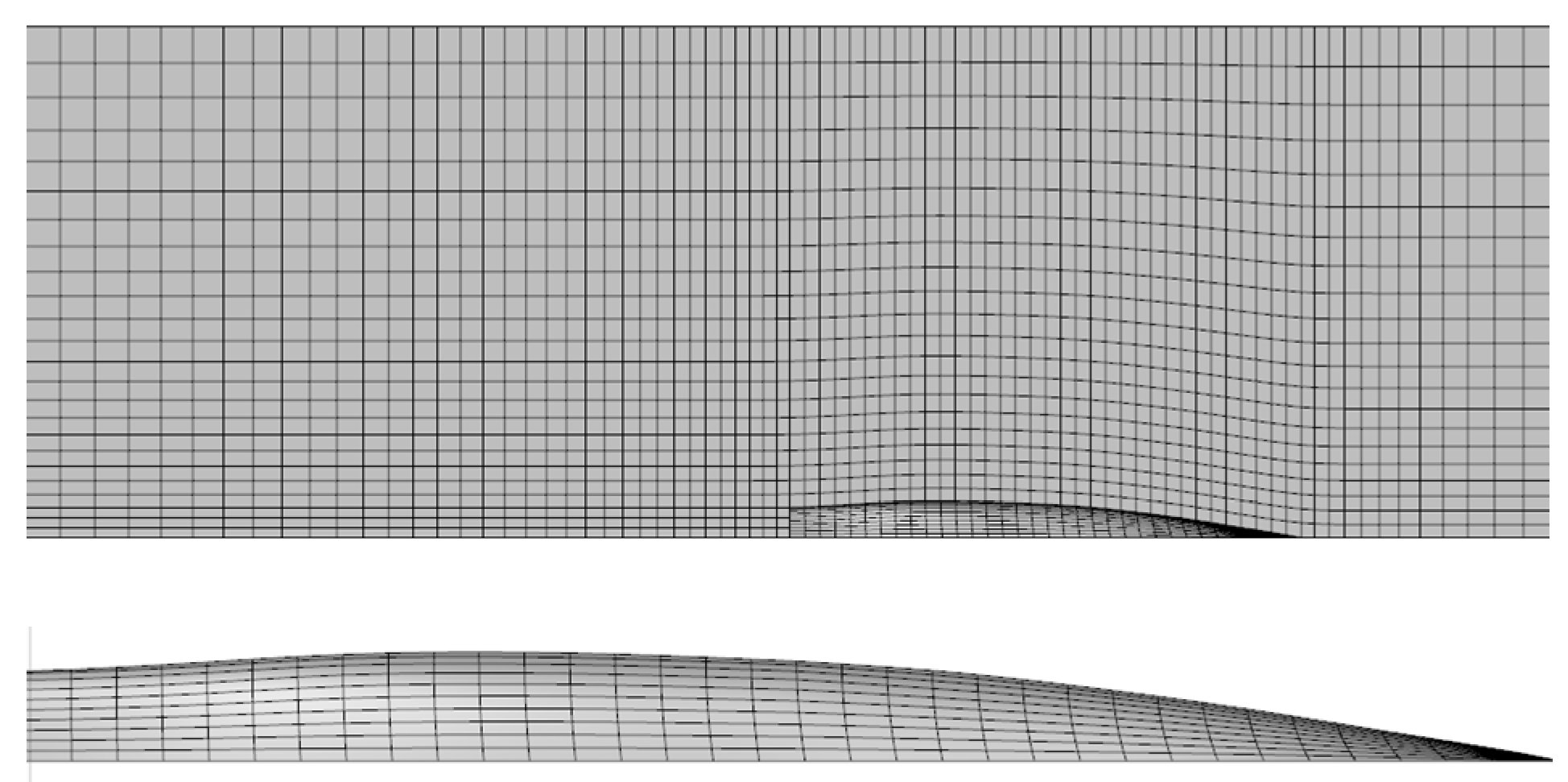
In the present method, a half hull and free surface were taken into account to decrease the number of panels used in calculating wave-making resistance. The half hull surface was formed from 740 panels (Figure 4). The free surface was a 3.5L_pp × 1.0L_pp ranged area with 1776 panels distributed which meets the panelization requirements mentioned by Janson [34] and Eslamdoost [14].

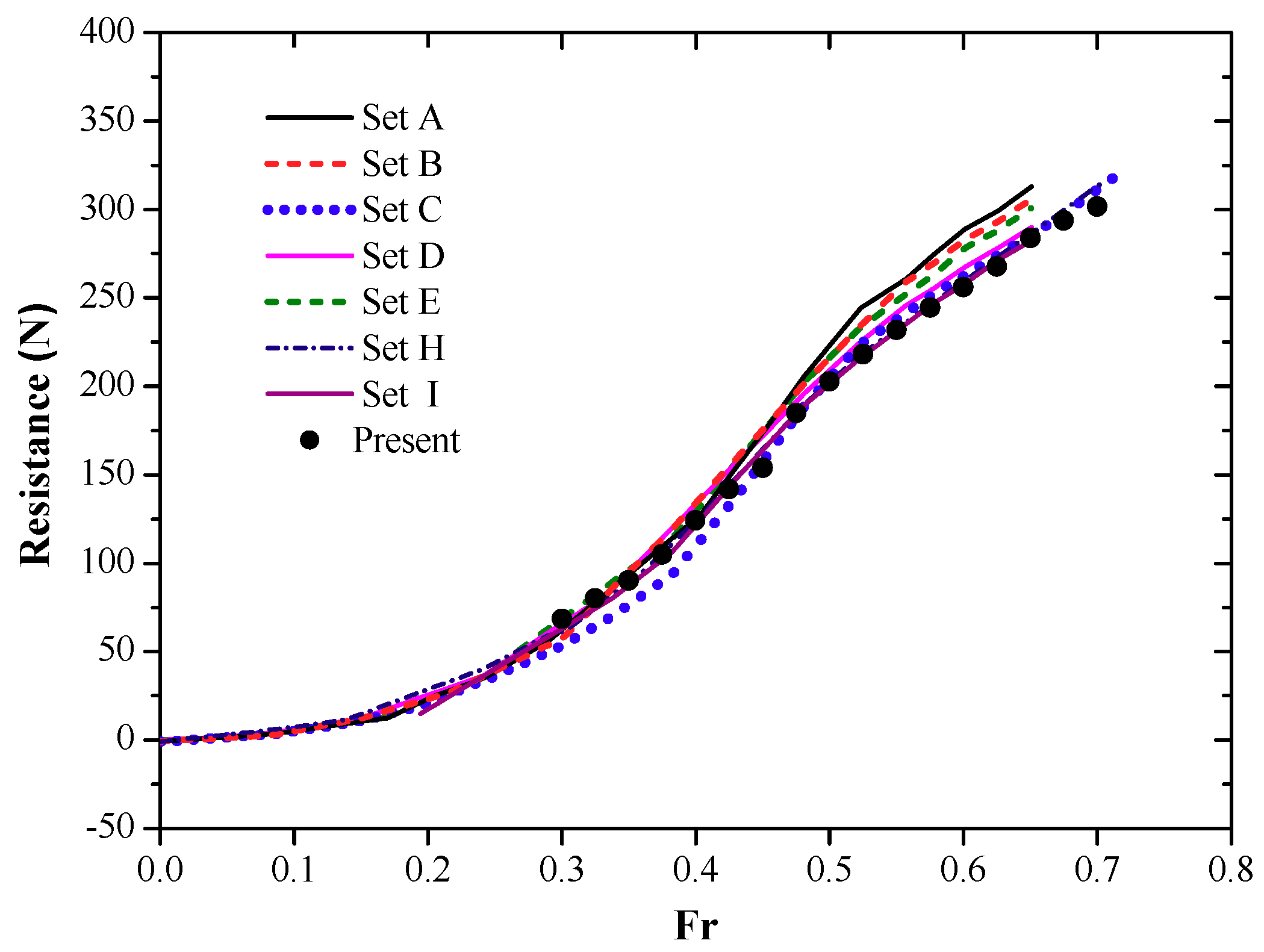
For barehull resistance, this method showed a good agreement with the EFD data at Fr = 0.3–0.5 in Figure 5. While Fr > 0.5, the computed resistance scatters were distributed near the Set C, D, H, and I curves. The mean error of the other three sets of EFD data was about 7% at Fr = 0.5–0.7.

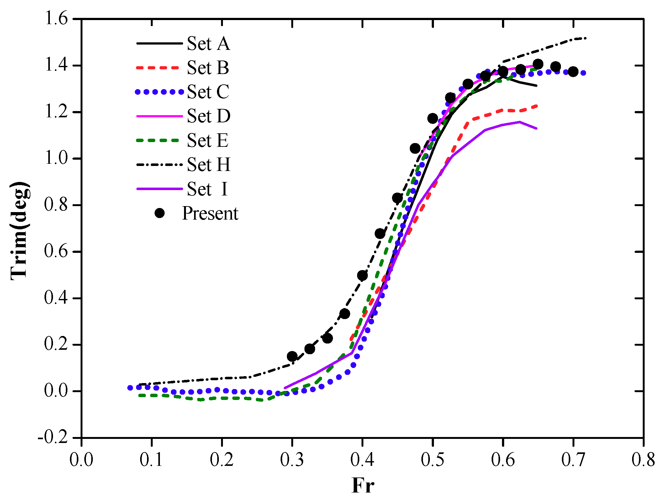
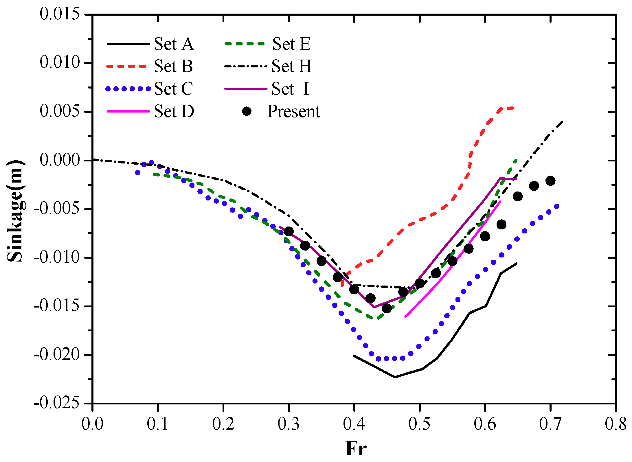
For Fr = 0.3–0.6, the calculated trim angle (Figure 6) had almost the same value as Set H, but was larger than the other data sets. The trim distribution trend line was fit with the mean EFD data. The computed sinkage reached the lowest point of −15 mm at Fr = 0.45 and matched the trend line of Set E, H, and I, as shown in Figure 7.

The noticeable distinction between the EFD data from the seven institutes mainly resulted from the non-uniform test conditions and differences in data measurements. The model differences of weight and temperature ranged from −2.6% to +3.9% and −20.7% to +14.7% compared with the mean values, respectively. Temperature determines the water density and viscosity, while weight determines the ship shape immersed in water. Furthermore, towing tanks of different sizes have been used by each institute. Different blocking effects significantly contributed to the observed differences. The joint effect of different factors led to a scatter in the experimental data. Despite the difference among the EFD data sets, their good agreement with the majority of the EFD data validates the present method for calculating ship resistance with free trim and sinkage.

4.2. Validation for Capture Area Parameters

The validation of the capture area parameters was carried out for two real ships mentioned in Jin’s [35], Zhang’s [36], and Liu’s papers [28]. The data for this calculation is listed in

Table 2. The main data of the real ship for validation.

	Speed (m/s)	Flow Volume (m3/s)	Distance Between the Inlet Point of the Tangency and Bow (m)
Ship 1	16.00	1.09	5.0
Ship 2	20.58	5.23	38.0

.

The results in

Table 3. Comparison of results between different methods.

	Method	δ (m)	W (m)	Y0 (m)	${\mathit{c}}_{\mathit{m}1\mathit{a}}$
Ship 1	Jin’s	0.0846	0.750	0.1342	0.9482
	Liu’s	0.0677	0.750	0.1241	0.9399
	Present	0.0651	0.750	0.1239	0.9414
Ship 2	Zhang’s	0.350	0.852	0.5160	0.8710
	Liu’s	0.451	0.852	0.4378	0.8752
	Present	0.338	0.852	0.4342	0.8809

show that the momentum coefficient c_m1a agrees well with the other methods for both two ships. For Ship 1, Y₀ and δ had a value closer to Liu’s results. For Ship 2, Y₀ was very similar to Liu’s results, and δ was closer to Zhang’s. The differences in the values of δ that occurred between the three methods was mainly due to the variety of dynamic viscosity and δ formulas. The validation results indicate that the present method gave a reasonable and acceptable calculation of parameters for the capture area.

4.3. Validation of Self-Propulsion for the Athena Ship

The ITTC waterjet self-propulsion experimental test for the waterjet Athena model was carried out at Fr = 0.6. The measured data included waterjet thrust, rope force, trim, sinkage, IVR, NVR, thrust deduction, etc. Among the data, only the reported scatter points were displayed in the following comparison figures. The numerical results from Eslamdoost [14] were taken as contrast for the present hybrid method in the self-propulsion validation procedure.

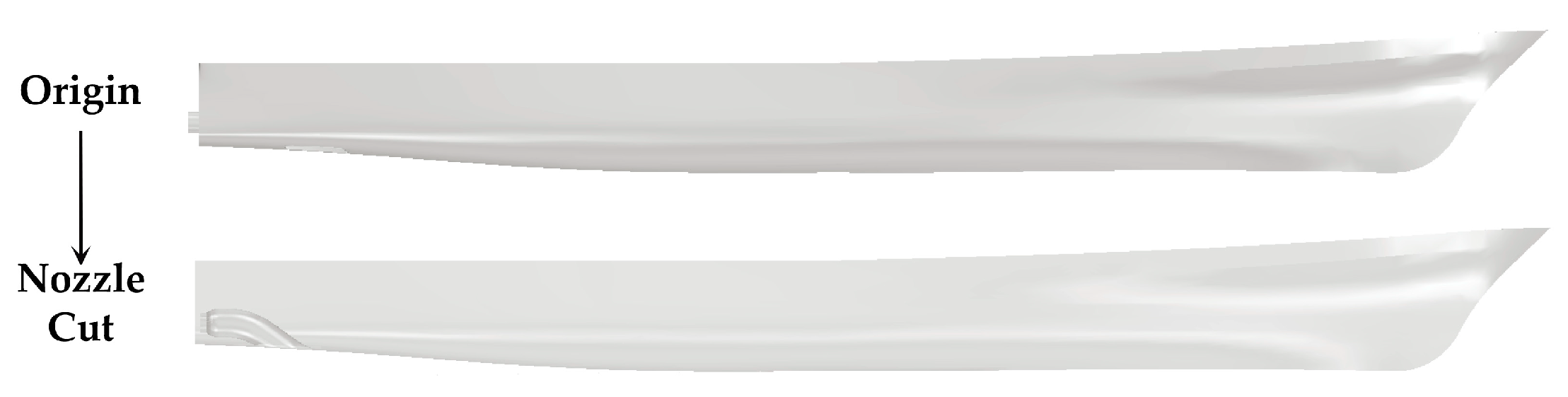
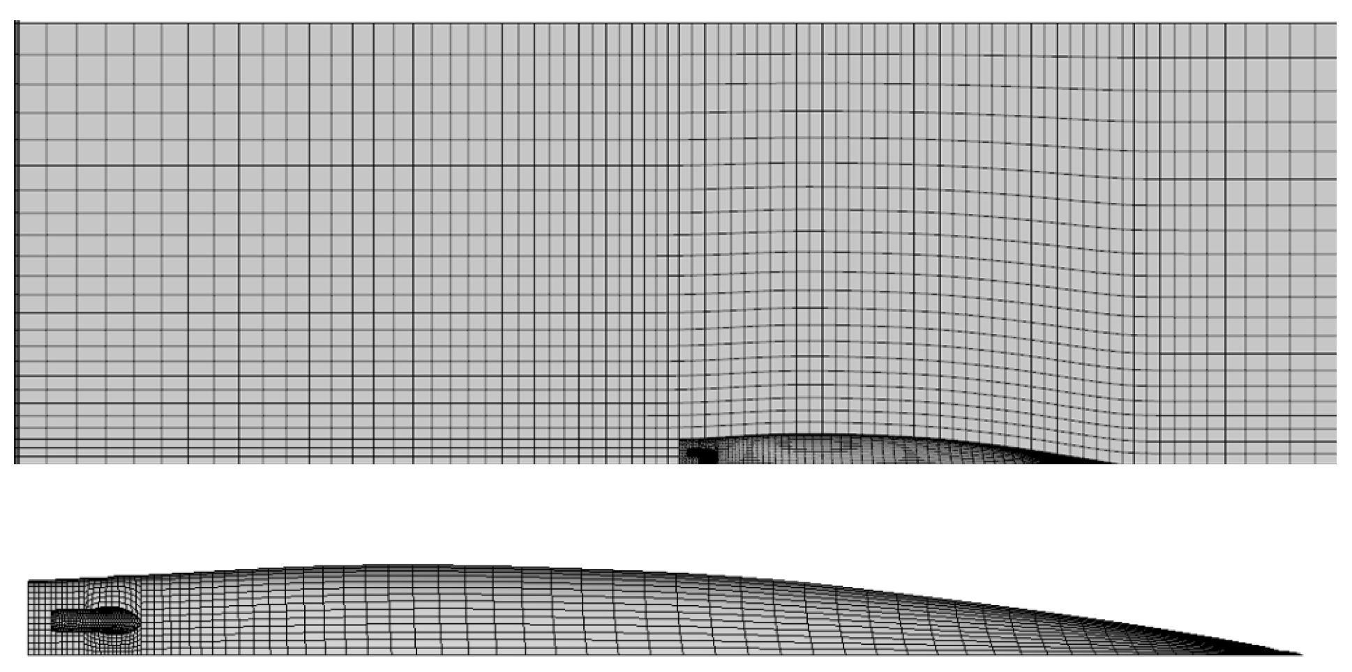
For the waterjet Athena model in the experiment, water flowed into the duct, passed through the transom, and then sprayed out from the nozzle. This process in the wave-making resistance calculation could not be achieved by using the boundary element method, which is based on the potential theory. Panel penetration between the free surface and nozzle at the stern results in a numerical error in the computation. To avoid this situation and proceed with the calculation, the Athena waterjet model was modified by cutting the outside part of the nozzle, as Figure 8 shows. Figure 9 displays the mesh of the free surface and the Athena hull with an intake duct.

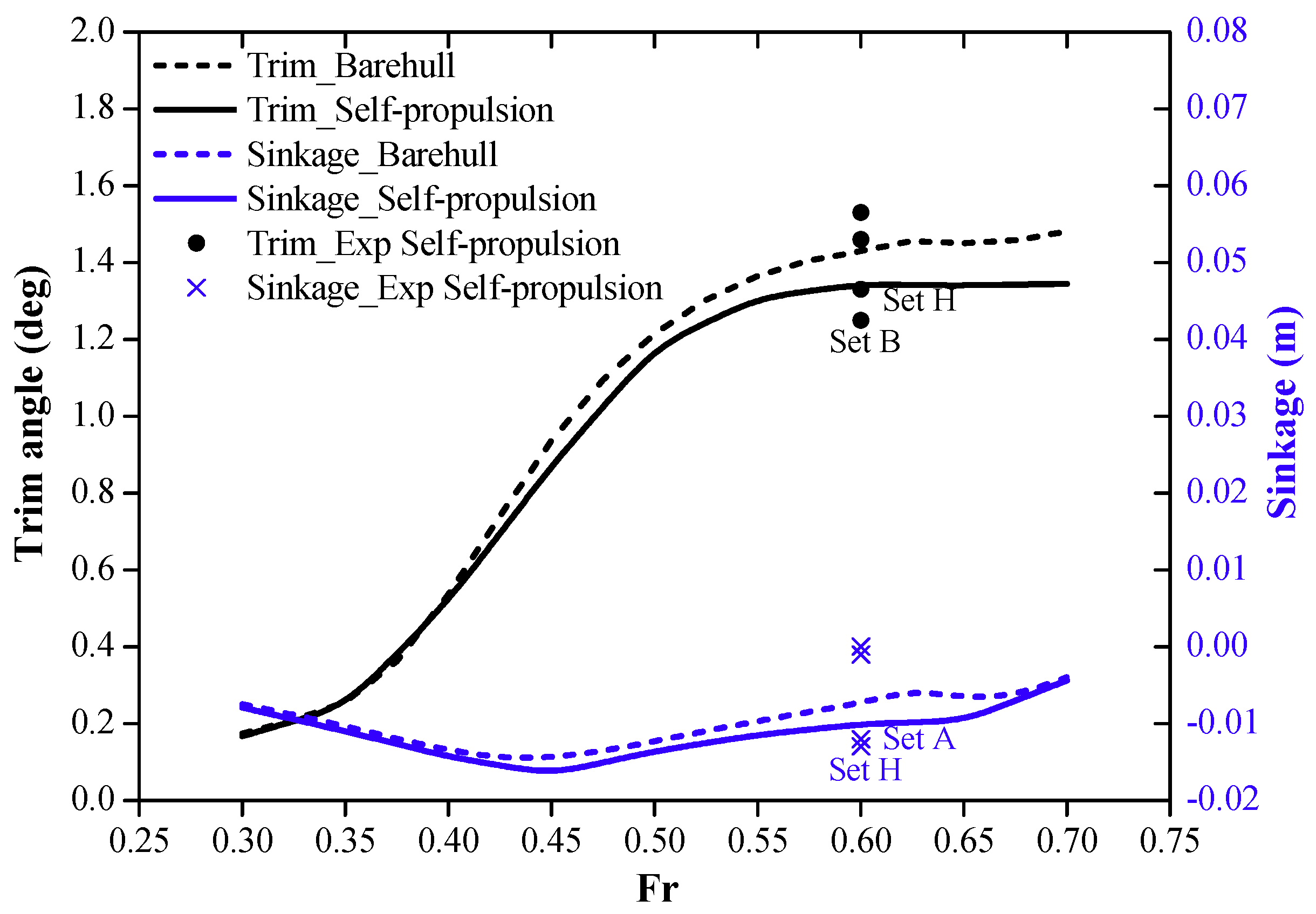
The waterjet self-propulsion was computed over the Fr range of 0.3–0.7 based on the present hybrid method. The trim and sinkage of the barehull and self-propulsion were compared in Figure 10. The trim under two conditions stayed almost the same at Fr < 0.4. However, when Fr > 0.4, the trim difference increased as the Fr increased, and the maximum gap reached 0.135° at Fr = 0.7. The two sinkage curves deviated from Fr = 0.4. The observed maximum difference was at Fr = 0.625. Data at Fr = 0.6 show that the computed trim was closer to the Set H data point, with a 0.26% error. The sinkage was closer to Set A and was 1.7 mm shallower. For the self-propulsion hull, the hydrodynamic force acting on the duct generated a forward moment which reduced the trim. Meanwhile, the low pressure distribution on the hull surface around the intake duct resulted in a deeper immersion.

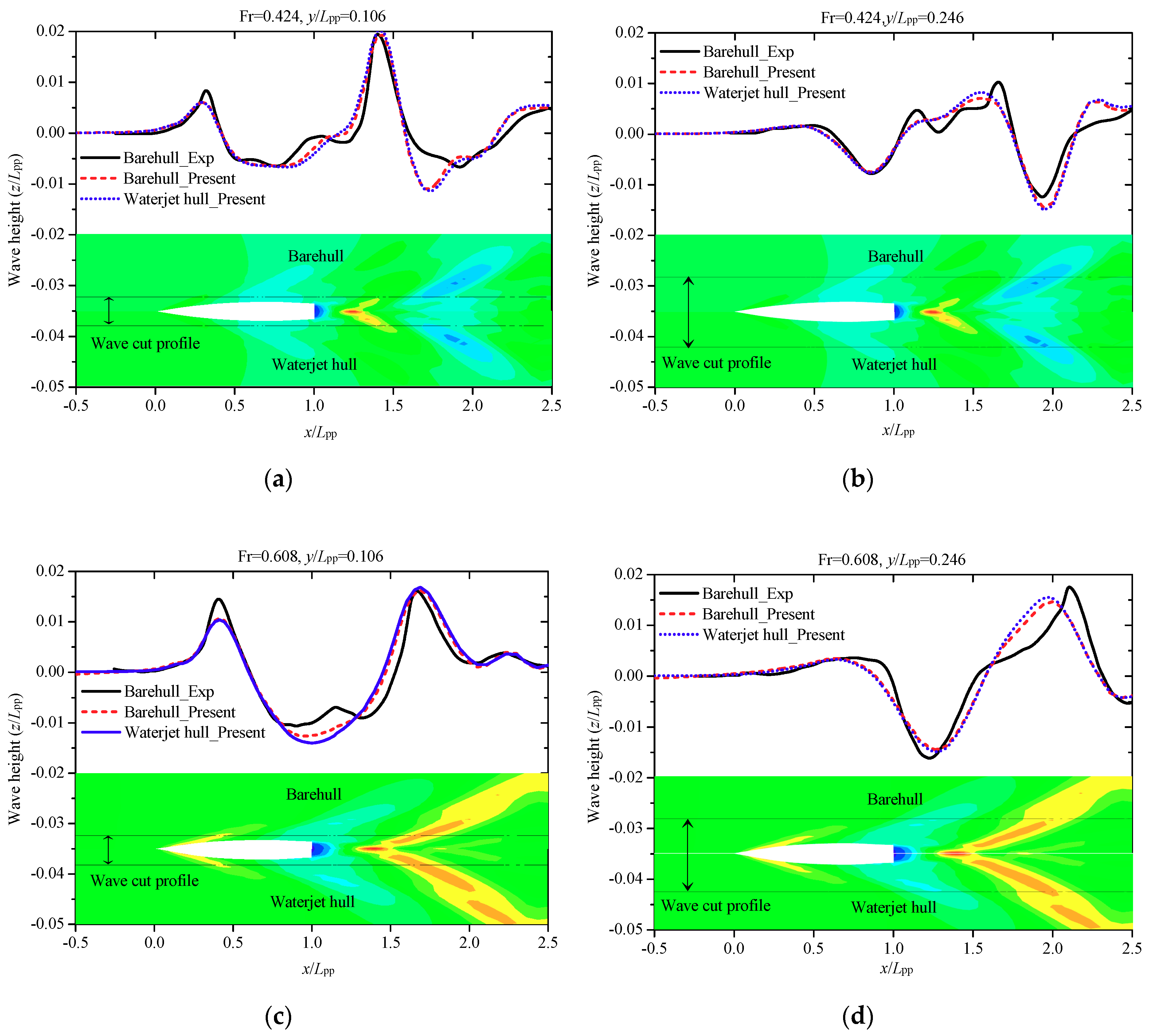
The wave cut profiles of the barehull and waterjet hull were generated in y/L_pp = 0.106, 0.246 at Fr values of 0.424 and 0.608. The experimental data was referenced from Fu’s model test report for the 1/8.25 model-scale Athena ship [29]. The four wave cut profiles showed the same trend with the measured results (The computed data has been converted using the coordinates of the model test), as illustrated in Figure 11. The peak and trough points matched well with the EFD curves. Even the wave fluctuation was observed after the stern, as shown in Figure 11b. As the nozzle was cut off outside the hull to ensure wave-making resistance computation went smoothly, the wave patterns at the stern showed a similar trend between the barehull and waterjet hull.

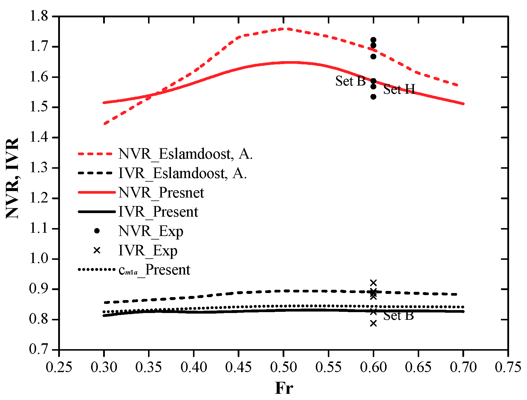
IVR and NVR are the important parameters of waterjet thrust in the momentum flux method. A sharp contrast of IVR and NVR values between the present method and the comparison results is illustrated in Figure 12. The reason for this difference is the consideration of the local loss coefficient in the present method, which resulted in the decrease of NVR in Equation (8). The present results had a lower value at Fr values of 0.35–0.7. Both the two NVR curves increased steadily and reached their peak at Fr = 0.5. The IVR value based on the boundary layer theory appears to be underestimated compared with the results of Eslamdoost [14], based on the viscous CFD method. The relationship between the δ and Y₀ curves illustrates that the capture area was located inside the boundary layer, which resulted in an underdeveloped velocity distribution in the capture area and the relatively lower position of IVR, as shown in Figure 12.

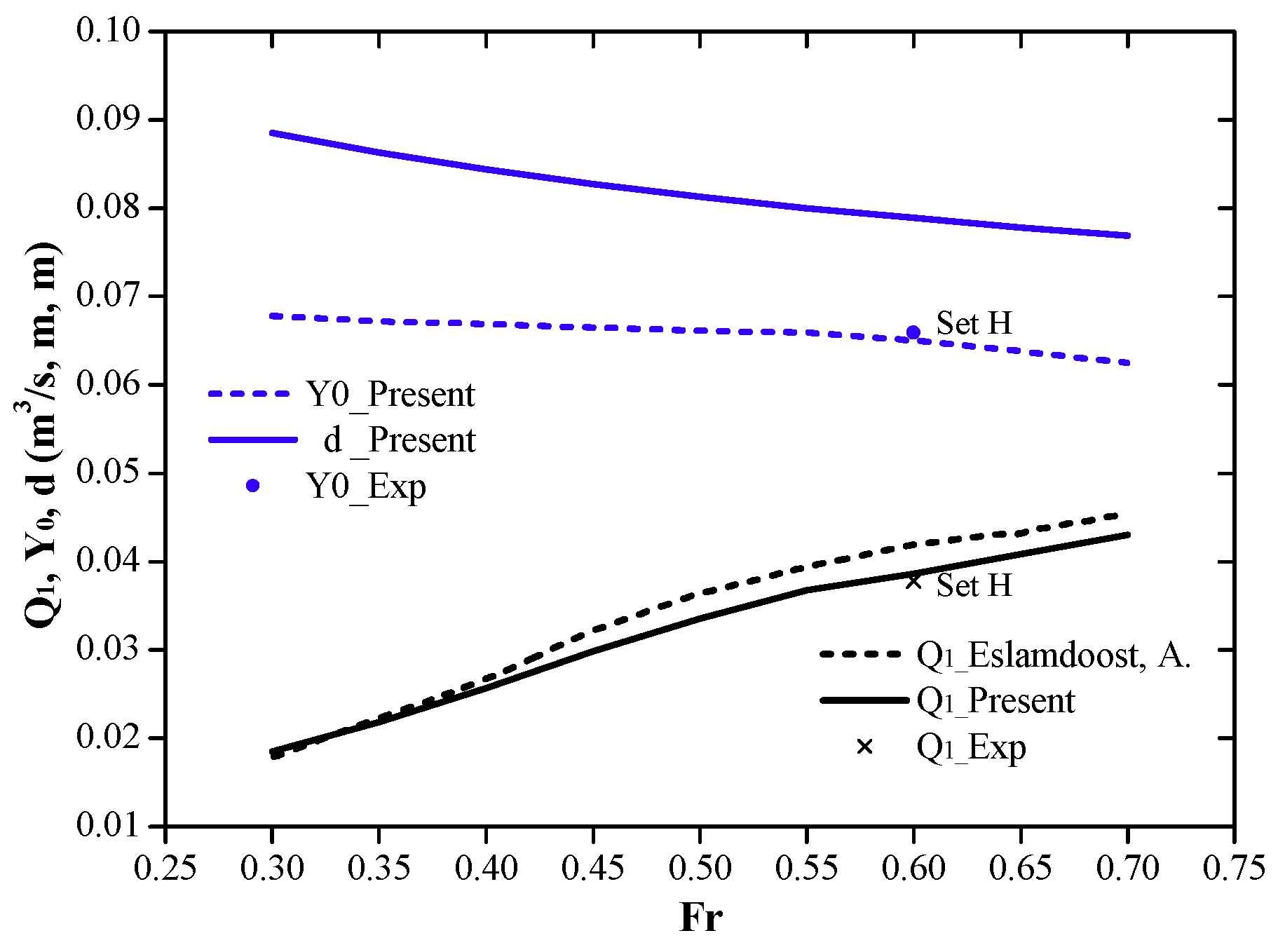
A good agreement between Q₁ and Y₀ was observed between the prediction and Set H data at Fr = 0.6 in Figure 13. This was despite the fact that the predicted Q₁ curve had an average 4.67% lower than the comparison curve.

Considering the influence of the boundary layer, in theory, the waterjet thrust calculated by the momentum flux method in the virtual control volume was:

$$T_g=N\rho Q_1(\overline{u_{m5}}-\overline{u_{m1a}})$$

(33)

where $\overline{u_{m1a}}$ and $\overline{u_{m5}}$ are the average momentum velocity at the capture area and nozzle discharge, respectively.

Hu and Zangeneh [37] researched the waterjet pump flow using the RANS CFD method. They calculated the momentum velocity of the pump nozzle discharge. $\overline{u_{m5}}$ was found to be 0.4% higher than the average volumetric velocity, $\overline{u_5}$. Regardless of the tiny difference between the two average velocities, $\overline{u_5}$ was used instead of $\overline{u_m}$ in Equation (33). The waterjet thrust formula was:

$$T_{g1}=N\rho Q_1{u}_0(NVR-c_{m1a})$$

(34)

While the assumption was equally applied to the capture area, $\overline{u_{m1a}}$ was taken as $\overline{u_{1a}}$. Equation (34) becomes:

$$T_{g2}=N\rho Q_1{u}_0(NVR-IVR)$$

(35)

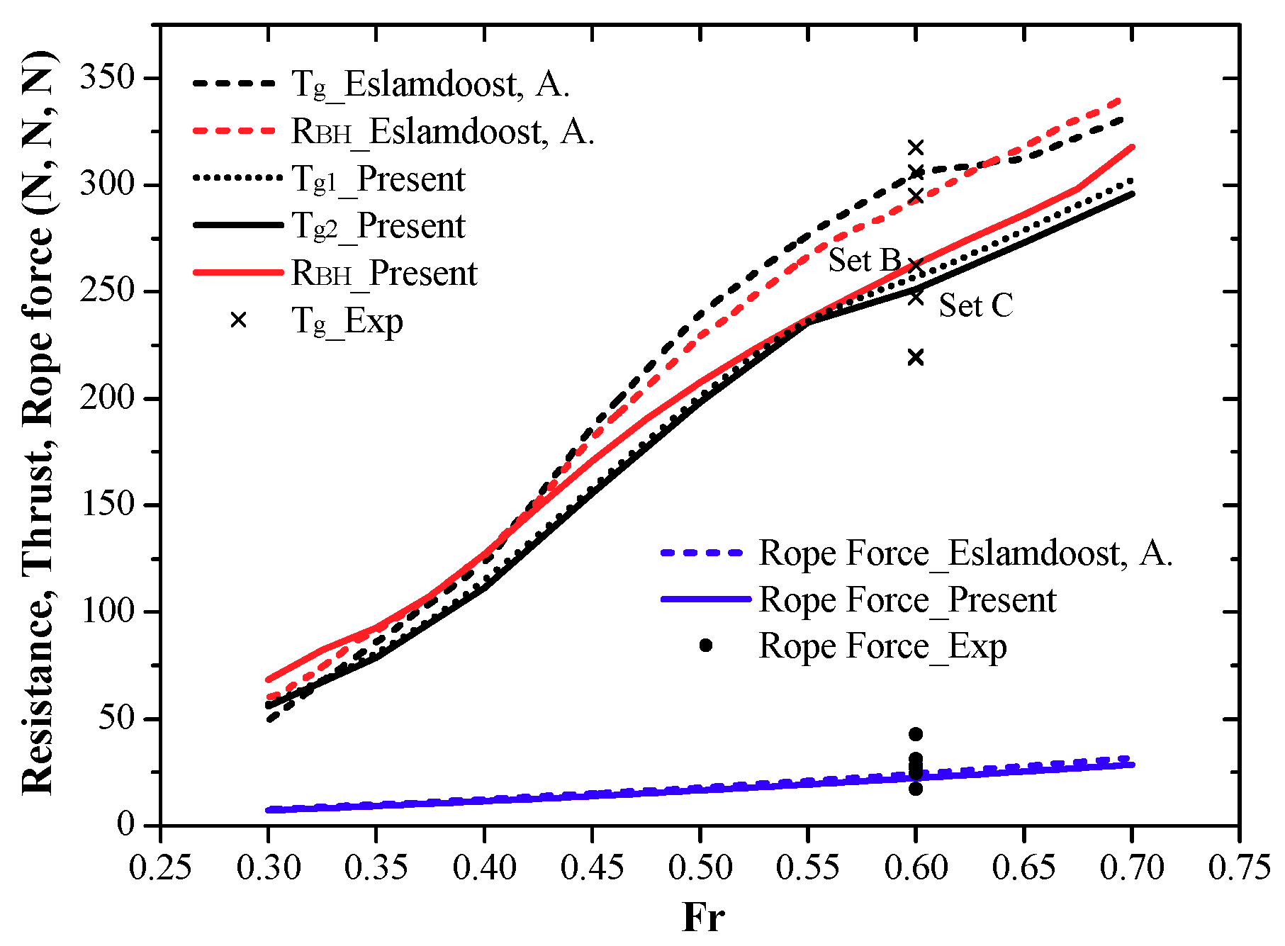
Equations (34) and (35) are the two widely used waterjet thrust formulas. In the present work, $c_{m1a}$ was 1.49% larger than IVR on average, as shown in Figure 12. The difference between the two formulas led to a 1.64% average discrepancy in waterjet thrust, as illustrated in Figure 14. The two waterjet thrust curves were more consistent with the Set B and C data at Fr = 0.6. As Eslamdoost uses a correction coefficient to correct the wave-making resistance during computation, the correction greatly increased the total resistance at high Froude numbers. Meanwhile, no correction was made in the present work as the calculated resistance was within the range of the experimental scatter, which resulted in the gap between the two resistance curves. A highly similar result for rope force was reported within the two curves and average EFD data.

The thrust deduction fraction prediction formula for the full-scale ship is:

$$t=1-\frac{R_{BH}-R_{rope}}{T_g}$$

(36)

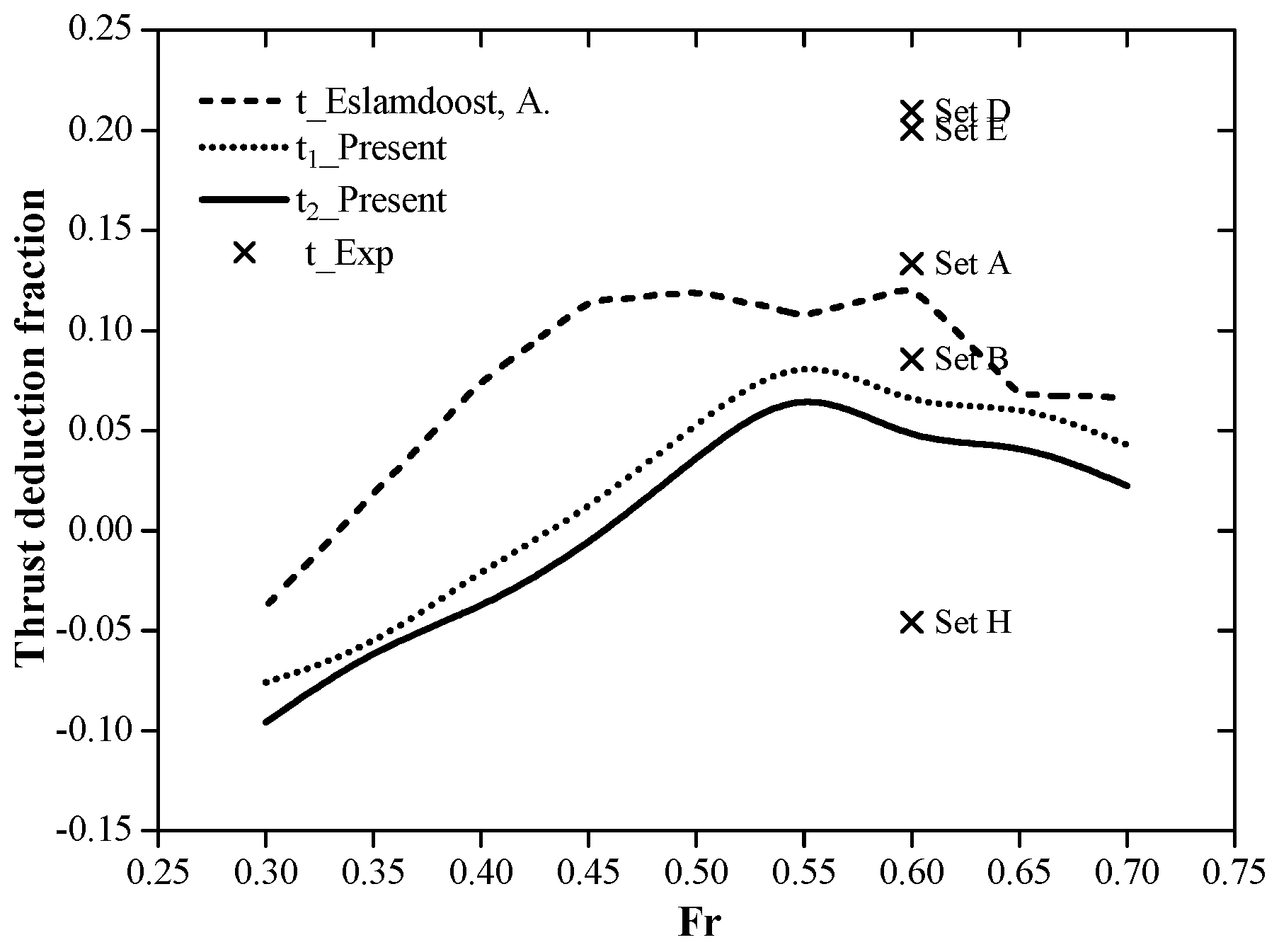
Two thrust deduction fraction curves were formed from the two waterjet thrust curves in the present method, which had a 1.65% difference in their averages, as shown in Figure 15. Negative thrust deduction occurred at Fr = 0.3–0.45, as the thrust deduction fraction increased steadily. The peak point was reached at Fr = 0.55. The thrust deduction fraction was underestimated in the present method compared with the average EFD data at Fr = 0.6, but this was within the scope of scatter.

Although some differences in the forces and deduction fraction were reported between the present hybrid method and the contrast data, in general the computation results generally met the experimental data well. The algorithm was validated to be applicable in a wide range of Froude number values, which could be applied to other ship types.

4.4. Application in the Side-Hull Configuration Research for a Trimaran

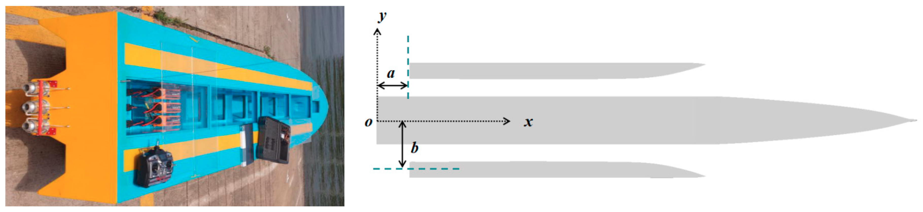
The target ship was a 120 m length waterjet-propelled trimaran with a service speed of 40 kn (Fr = 0.6). A 1/30 scale ship model was constructed, as shown in Figure 16. The previous research on the side-hull configuration was focused on added mass research [23,24] and resistance based optimization [38,39]. As the hybrid method was validated on the Athena mono ship, the waterjet performance based side-hull configuration research for the trimaran model was numerically performed at Fr = 0.3–0.6 using the discussed method. The side-hull layout parameters and main data of the trimaran are provided in Figure 16 and

Table 4. The main data of the trimaran and side-hull layout.

	Main Hull Length (m)	Main Hull Breadth (m)	Draught (m)	Side-Hull Length (m)
Full-scale	120.0	10.50	3.6	67.00
Model-scale	4.0	0.35	0.12	2.23
Side-Hull Parameters
a/Lpp	–0.25	0.00	0.25	0.50
b/Lpp	0.10	0.15	0.20	0.25

.

Depending on the design, four positions were used in both the longitudinal (a/L_pp) and transverse (b/L_pp) directions, resulting in a total of 16 different side-hull layouts. Both the barehull and waterjet hull were used in the same side-hull configuration to generate a mesh and compute the waterjet performance.

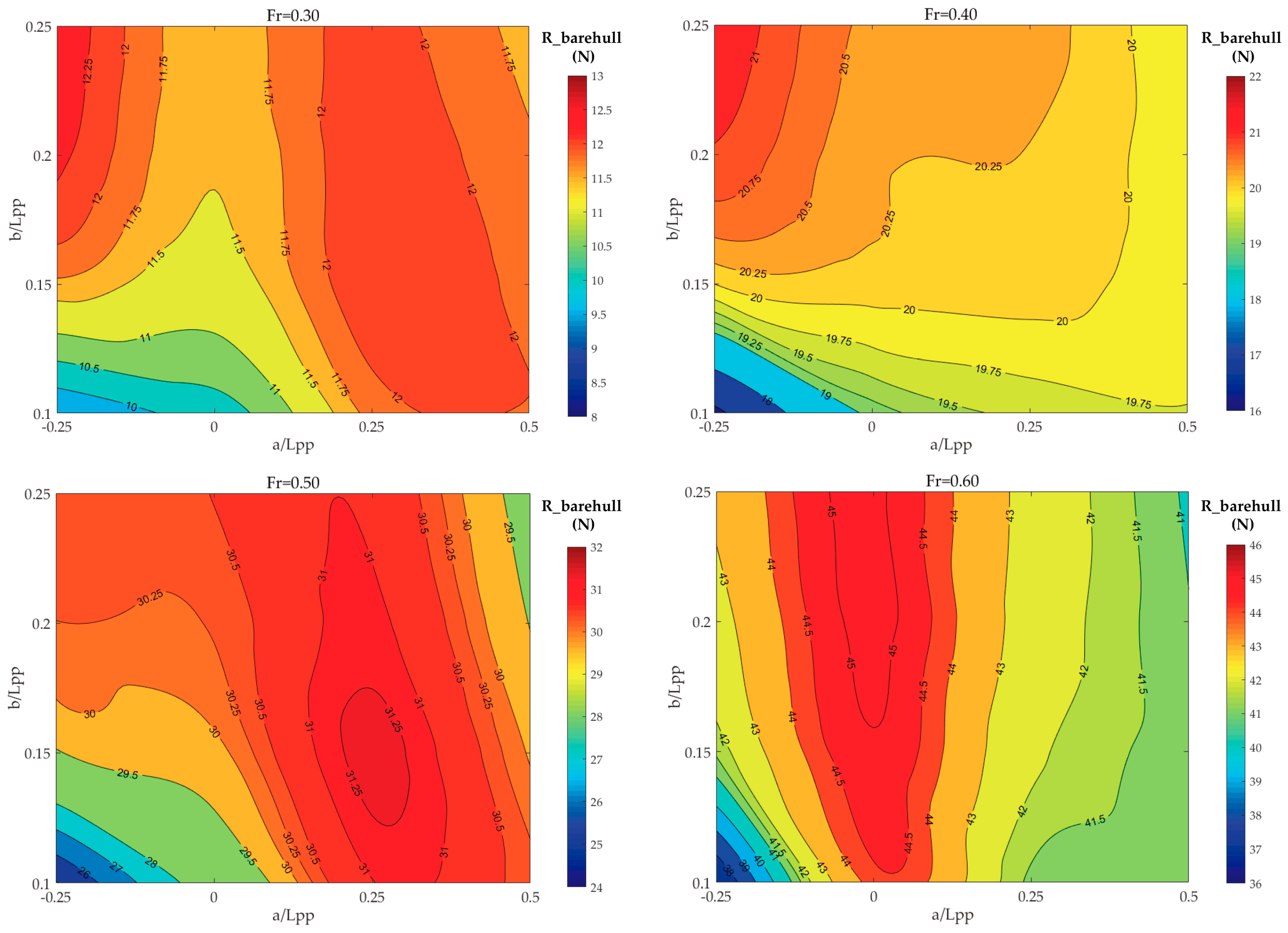
The barehull resistance was computed based on the barehull model. Figure 17 shows the resistance distribution of different side-hull layouts. Evidently, in the range of Fr = 0.3–0.6, the side-hull located at a/L_pp = −0.25 had an obvious advantage of low drag in the longitudinal position. Meanwhile, the smaller the lateral position of the side-hull, the closer the side-hull was to the main hull. The closer the side-hull was to the main hull, the better the drag reduction. This low-resistance layout distribution is well understood. When a/L_pp < 0, a part of the side body beyond the main hull transom is equivalent to an increase in the “effective ship length”, which is beneficial to the reduction of the wave-making resistance. When the body is laterally close to the main hull, the “effective ship width” of the trimaran is reduced and the trimaran becomes more slender, which is also contributes to the wave-making resistance reduction. It is worth noting that, at a high speed of Fr = 0.6, the trimaran with a side-hull located at a/L_pp = 0.5 near the bow (i.e., a ”fore-body trimaran” [40]), shows the characteristics of reduced resistance. This is shown in Figure 17, which is consistent with the conclusions obtained in the model test in Jia’s paper [40].

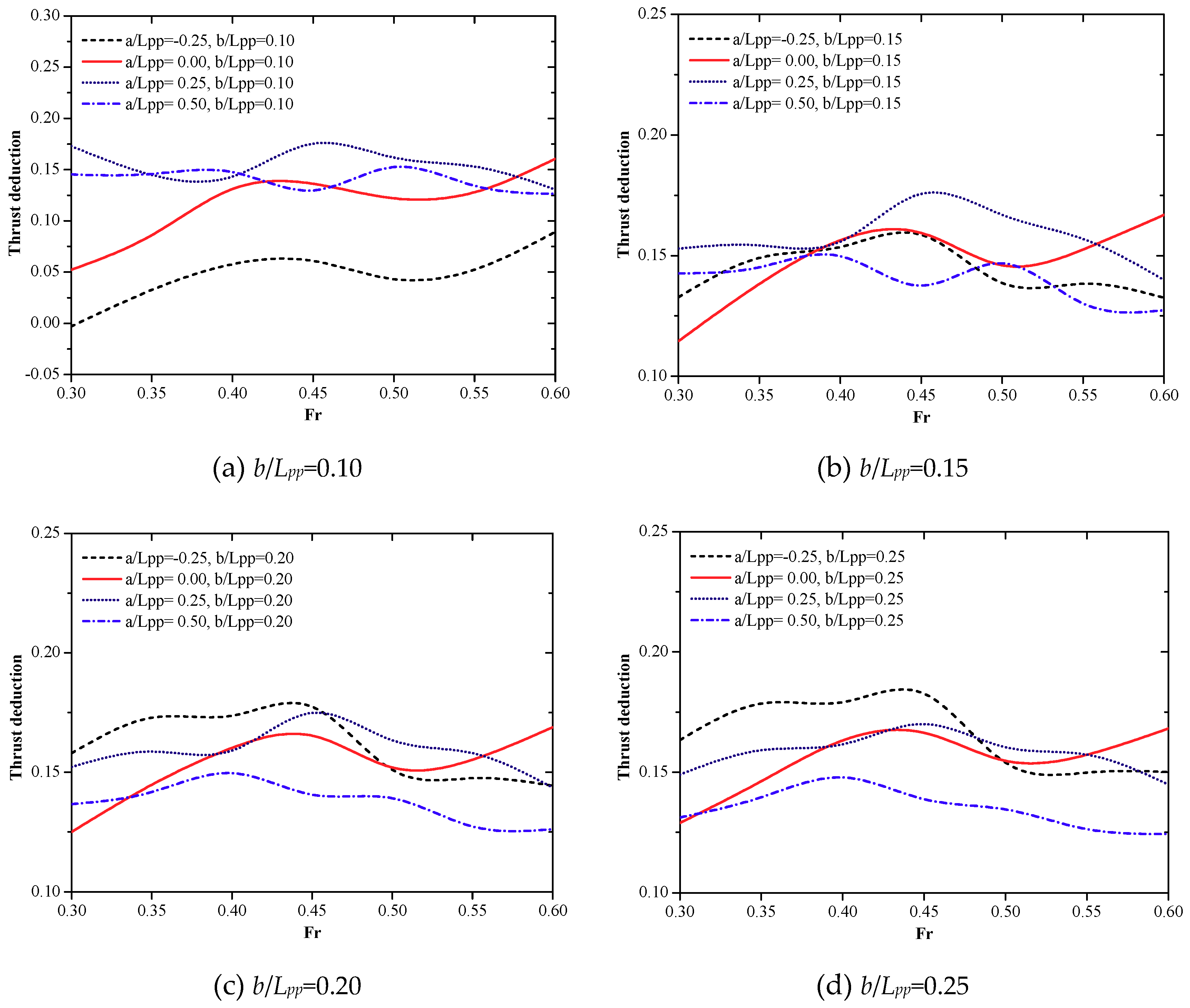
Waterjet thrust and other parameters were calculated using the waterjet hull models. Then, the thrust deduction was obtained using Equation (36), and the thrust deduction with the Fr distribution curve is shown in Figure 18.

Similar to what was shown regarding resistance distribution, Figure 18a shows that the trimaran with a side-hull located at a/L_pp = −0.25, b/L_pp = −0.1 had an advantage in thrust deduction, which means this side-hull layout has an efficient propulsion performance. As displayed in Figure 18c,d, when b/L_pp > 0.2, the “fore-body trimaran” had the lowest thrust deduction at Fr > 0.35.

5. Conclusions

The hybrid method for determining wave-making resistance, viscous resistance, and capture area physical quantities was proposed to calculate waterjet propulsion performance using iterative computation. The validation process for the barehull, capture area, and self-propulsion was applied. The differences of the IVR, NVR, resistance, waterjet thrust, and thrust deduction fraction values between the present method and contrast results were discussed. In the results of the present study, the lower NVR was obtained by considering the local loss in the iteration equation. This shows a 0.2% error compared to the EFD Set B data. As the location of the computed capture area was inside the boundary layer, the lower IVR was obtained, which had a 0.4% difference compared to the EFD Set B data. The error of waterjet thrust was 2.5% compared with the EFD Set B data. Although the differences exist, the present work showed similar tendencies in the comparison curves and reached a good agreement with the experimental data. A comparison between two widely used waterjet thrust formulas was investigated while using the volumetric inlet velocity instead of the momentum inlet velocity. On average, their difference and that of the waterjet thrust and thrust deduction was 1.49%, 1.64%, and 1.65%, respectively.

In addition, the application of the hybrid method in the side-hull configuration research further verified the applicability of the present method. While the side-hull position of the trimaran was located on the rear side of the main hull, its layout was conducive to energy-saving and efficient waterjet propulsion performance. Furthermore, if a large deck area was required and the side-hull was relatively far from the main hull, the layout of the “fore-body trimaran” could be selected to reduce the drag and thrust deduction at a high Froude number.

The hybrid method presented in this paper was preliminarily verified as an effective way to research and predict the characteristics of waterjet propulsion without considering the impeller rotation and cavitation. Research on more waterjet hull types and applications based on the hybrid approach will be undertaken in further works.

References

- Van, T.T. The effect of waterjet-hull interaction on thrust and propulsive efficiency. In Proceedings of the FAST’91, Trondheim, Norway, 17–21 June 1991. [Google Scholar]
- Alexander, K.; Coop, H.; Terwisga, T. Waterjet-Hull interaction: Recent experimental results. SNAME Trans. 1993, 102, 275–335. [Google Scholar]
- Allison, J. Marine waterjet propulsion. SNAME Trans. 1993, 101, 275–335. [Google Scholar]
- Okamoto, Y.; Sugioka, H.; Kitamura, Y. On the pressure distribution of a waterjet intake duct in self propulsion conditions. In Proceedings of the FAST’93, Yokohama, Japan, 13–16 December 1993; pp. 843–854. [Google Scholar]
- ITTC. The specialist committee on waterjets. Final report and recommendations to the 21st ITTC. In Proceedings of the 21st International Towing Tank Conference, Trondheim, Norway, 15–21 September 1996. [Google Scholar]
- Watson, S.J.P. The Use of CFD in sensitivity studies of inlet design. In Proceedings of the RINA International Conference on Waterjet Propulsion, Amsterdam, The Netherlands, 22–23 October 1998. [Google Scholar]
- Roberts, J.L.; Walker, G.J. Boundary layer ingestion effects in flush waterjet intakes. In Proceedings of the RINA International Conference on Waterjet Propulsion, Amsterdam, The Netherlands, 22–23 October 1998. [Google Scholar]
- Kimball, R.W. Experimental Investigations and Numerical Modeling of a Mixed Flow Marine Waterjet; Massachusetts Institute of Technology: Cambridge, MA, USA, 2001. [Google Scholar]
- Park, W.G.; Jang, J.H.; Chun, H.H.; Kim, M.C. Numerical flow and performance analysis of waterjet propulsion system. Ocean Eng. 2004, 32, 1740–1761. [Google Scholar] [CrossRef]
- Park, W.G.; Yun, H.S.; Chun, H.H.; Kim, M.C. Numerical flow simulation of flush type intake duct of waterjet. Ocean Eng. 2005, 32, 2107–2120. [Google Scholar] [CrossRef]
- Takai, T. Simulation Based Design for High Speed Sea Lift with Waterjets by High Fidelity URANS Approach; University of Iowa: Iowa City, IA, USA, 2010. [Google Scholar]
- Takai, T.; Kandasamy, M.; Stern, F. Verification and validation study of URANS simulations for an axial waterjet propelled large high-speed ship. J. Mar. Sci. Technol. 2011, 16, 434–447. [Google Scholar] [CrossRef]
- Altosole, M.; Benvenuto, G.; Figari, M.; Campora, U. Dimensionless numerical approaches for the performance prediction of marine waterjet propulsion units. Int. J. Rotat. Mach. 2012, 2012, 321306. [Google Scholar] [CrossRef]
- Eslamdoost, A. The Hydrodynamics of Waterjet/hull Interaction; Chalmers University of Technology: Chalmers, Sweden, 2014. [Google Scholar]
- Eslamdoost, A.; Larsson, L.; Bensow, R. Net and gross thrust in waterjet propulsion. J. Ship Res. 2016, 60, 1–14. [Google Scholar] [CrossRef]
- Li, Y.B.; Gong, J.Y.; Ma, Q.W.; Yan, S.Q. Effects of the terms associated with ϕzz in free surface condition on the attitudes and resistance of different ships. Eng. Anal. Bound. Elem. 2018, 95, 266–285. [Google Scholar] [CrossRef]
- Chybowski, L.; Grządziel, Z.; Gawdzińska, K. Simulation and experimental studies of a multi-tubular floating sea wave damper. Energies 2018, 11, 1012. [Google Scholar] [CrossRef]
- Frederick, S.; Wang, Z.Y.; Yang, J.; Sadat-Hosseini, H.; Mousaviraad, M.; Bhushan, S.; Diez, M.; Yoon, S.H.; Wu, P.C.; Yeon, S.M.; et al. Recent progress in CFD for naval architecture and ocean engineering. J. Hydrodyn. 2015, 27, 1–23. [Google Scholar]
- ITTC. The specialist committee on validation of waterjet test procedures: Final report and recommendations to the 24th ITTC. In Proceedings of the 24th International Towing Tank Conference, Edinburgh, UK, 4–10 September 2005. [Google Scholar]
- Xia, Q.C. Engineering Fluid Mechanics; Shanghai Jiao Tong University Press: Shanghai, China, 2006; pp. 210–213. [Google Scholar]
- Zhou, L.L. Numerical Study of High Speed Ship Tail Wave; Wuhan University of Technology: Wuhan, China, 2012. [Google Scholar]
- Tarafder, M.S.; Suzuki, K. Numerical calculation of free-surface potential flow around a ship using the modified Rankine source panel method. Ocean Eng. 2008, 35, 536–544. [Google Scholar] [CrossRef]
- Zhang, L.; Zhang, J.N.; Zhang, H.J.; Shang, Y.C. Numerical research on the added mass of trimaran from transition state to semi-planing state based on the boundary element method. In Proceedings of the ISOPE 2017, San Francisco, CA, USA, 25–30 June 2017; pp. 984–989. [Google Scholar]
- Zhang, L.; Zhang, J.N.; Dong, G.X.; Chen, W.M. Numerical study on the influence of trimaran layout on added mass in semi-planing state. J. Dalian Marit. Univ. 2017, 43, 1–5. [Google Scholar]
- Tarafder, M.S.; Khalil, G.M. Calculation of ship sinkage and trim in deep water using a potential based panel method. Int. J. Appl. Mech. Eng. 2006, 11, 401–414. [Google Scholar]
- Wan, Z.; Liu, X.P.; Fu, P. Calculation of the sinkage and trim of trimaran and their effect on wave making resistance. J. Shanghai Jiaotong Univ. 2010, 44, 1388–1392. [Google Scholar]
- Hou, Y.H.; Huang, S.; Liang, X. Ship hull optimization based on PSO training FRBF neural network. J. Harbin Eng. Univ. 2017, 38, 175–180. [Google Scholar]
- Liu, Z.L.; Yu, R.T.; Zhu, Q.D. Study of a method for calculation boundary layer influence coefficients of ship and boat propelled by water-jet. J. Ship Mech. 2012, 16, 1115–1121. [Google Scholar]
- Fu, T.C.; Karion, A.; Pence, A.; Rice, J.; Walker, D.; Ratcliffe, T. Characterization of the Steady Wave Field of the High Speed Transom Stern Ship-Model 5365 Hull Form; Hydromechanics Department Report; Carderock Division Naval Surface Warface Center: Bethesda, MD, USA, 2005. [Google Scholar]
- Bhushan, S.; Xing, T.; Carrica, P.; Stern, F. Model- and full-scale URANS simulations of Athena resistance, powering, seakeeping, and 5415 maneuvering. J. Ship Res. 2009, 53, 179–198. [Google Scholar]
- Wyatt, D.C.; Fu, T.C.; Taylor, G.L.; Terill, E.J.; Xing, T.; Bhushan, S.; O’Shea, T.T.; Dommermuth, D.G. A comparison of full-scale experimental measurements and computational predictions of the transom-stern wave of the R/V Athena I. In Proceedings of the 27th Symposium on Naval Hydrodynamics, Seoul, Korea, 5–10 October 2008. [Google Scholar]
- Hurwitz, R.B.; Crook, L.B. Analysis of Wake Survey Experimental Data for Model 5365 Representing the R/V Athena in the DTNSRDC Towing Tank; David W. Taylor Navel Ship Research and Development Center: Bethesda, MD, USA, 1980. [Google Scholar]
- William, G.; Day, J.; Reed, A.M.; Hurwitz, R.B. Full-Scale Propeller Disk Wake Survey and Boundary Layer Velocity Profile Measurements on the 154-Foot Ship R/V Athena; David W. Taylor Navel Ship Research and Development Center: Bethesda, MD, USA, 1980. [Google Scholar]
- Janson, C.E. Potential Flow Panel Methods for the Calculation of Free-Surface Flows with Lift; Chalmers University of Technology: Chalmers, Sweden, 1997. [Google Scholar]
- Jin, P.Z. Waterjet Propulsion for Ships; National Defense Industry Press: Beijing, China, 1986. [Google Scholar]
- Zhang, Z.; Wang, L.X. Estimation for inlet boundary layer affect coefficient around waterjet duct. Ship Boat 2008, 3, 9–14. [Google Scholar]
- Hu, P.; Zangeneh, M. CFD calculation of the flow through a waterjet pump. In Proceedings of the International Conference on Waterjet Propulsion III, RINA, Gothenburg, Sweden, 20–21 February 2001. [Google Scholar]
- Zhang, L.; Zhang, J.N. Optimization Research on the Side Hull Configuration and Position of Trimaran Based on Orthogonal Design Method. J. Wuhan Univ. Technol. Transp. Sci. Eng. 2015, 39, 747–750. [Google Scholar]
- Jin, M.X.; Zhang, J.N.; Zhang, L. Outrigger hulls’ position optimization based on resistance numerical simulation for trimaran. J. Dalian Marit. Univ. 2015, 41, 15–18. [Google Scholar]
- Jia, J.P.; Zong, Z.; Zhang, W.P. Fore-Body trimaran and experimental study of its resistance and motion characteristics. Chin. J. Ship Res. 2011, 6, 9–14. [Google Scholar]
Figure 1.
Definitions of the reference stations of the waterjet vessel.
Figure 2.
Iteration illustration of the waterjet thrust and thrust deduction.
Figure 3.
The relationship between effective thickness Y0 and the boundary layer.
Figure 4.
Mesh of the free surface and the Athena barehull model.
Figure 5.
Barehull resistance of the present method and the International Towing Tank Conference (ITTC) experimental fluid dynamics (EFD) data.
Figure 6.
Trim angle of the present method and the ITTC EFD data.
Figure 7.
Sinkage of the present method and the ITTC EFD data.
Figure 8.
Modification of the Athena waterjet model.
Figure 9.
Mesh of the free surface and the Athena waterjet model.
Figure 10.
Calculated trim and sinkage of the barehull and self-propulsion.
Figure 11.
Wave cut profiles: (a) Fr = 0.424, y/Lpp = 0.106; (b) Fr = 0.424, y/Lpp = 0.246; (c) Fr = 0.608, y/Lpp = 0.106; (d) Fr = 0.608, y/Lpp = 0.246.
Figure 12.
Comparison of IVR and NVR.
Figure 13.
The distribution of Q1, Y0, and δ.
Figure 14.
Comparison of the resistance, thrust, and rope force.
Figure 15.
The thrust deduction fraction.
Figure 16.
The trimaran model and side-hull configuration parameters.
Figure 17.
Barehull resistance distribution at different Froude numbers.
Figure 18.
Waterjet thrust deduction fraction curves of different side-hull layouts.