On the Assessment of Numerical Wave Makers in CFD Simulations


1
Centre for Ocean Energy Research, Maynooth University, W23 Maynooth, Co. Kildare, Ireland
2
Department of Fluid Mechanics, Budapest University of Technology and Economics, H-1111 Budapest, Hungary
3
Marine Research Group, Queen’s University Belfast, Belfast BT9 5AG, UK
*
Author to whom correspondence should be addressed.
J. Mar. Sci. Eng. 2019, 7(2), 47; https://doi.org/10.3390/jmse7020047
Submission received: 21 December 2018
/
Revised: 3 February 2019
/
Accepted: 5 February 2019
/
Published: 13 February 2019
(This article belongs to the Special Issue Computational Fluid Dynamics for Ocean Surface Waves)
Abstract
:A fully non-linear numerical wave tank (NWT), based on Computational Fluid Dynamics (CFD), provides a useful tool for the analysis of coastal and offshore engineering problems. To generate and absorb free surface waves within a NWT, a variety of numerical wave maker (NWM) methodologies have been suggested in the literature. Therefore, when setting up a CFD-based NWT, the user is faced with the task of selecting the most appropriate NWM, which should be driven by a rigorous assessment of the available methods. To provide a consistent framework for the quantitative assessment of different NWMs, this paper presents a suite of metrics and methodologies, considering three key performance parameters: accuracy, computational requirements and available features. An illustrative example is presented to exemplify the proposed evaluation metrics, applied to the main NWMs available for the open source CFD software, OpenFOAM. The considered NWMs are found to reproduce waves with an accuracy comparable to real wave makers in physical wave tank experiments. However, the paper shows that significant differences are found between the various NWMs, and no single method performed best in all aspects of the assessment across the different test cases.
1. Introduction
A numerical wave tank (NWT) is a generic name for numerical tools used to simulate free surface waves, hydrodynamic forces and floating body motions [1]. In the field of offshore and marine engineering, NWT experiments are a valuable tool used alongside physical wave tanks (PWT). Costs for experiments in NWTs and PWTs are highly case dependent [2]; however, NWTs have seen a large increase in application in recent years due to the ever increasing available cheap computational power, while offering access to all field variables and flexibility in tank layout and experimental design.
1.1. Computational Fluid Dynamics-Based Numerical Wave Tanks
The accuracy of a NWT is driven by the underlying numerical modelling approach, which is often simplified in order to reduce the computational burden. Low fidelity models, e.g., potential flow-based NWTs, implementing the Laplace equation, are able to compute results with minimal computational cost and are valuable for parametric studies (see examples in [1,3]). However, due to the underlying assumptions of inviscid fluid and small amplitude wave and body motion, the range over which these models are valid is often exceeded for offshore and marine engineering applications. Compared to lower fidelity numerical tools, high-fidelity numerical models, such as CFD-based NWTs (CNWTs), have the advantage of capturing relevant hydrodynamic non-linearities, such as complex free surface elevation (including wave breaking), viscous drag and turbulence effects. Although CNWTs are more computationally costly than their lower fidelity counterparts, CNWT experiments can deliver accurate results in high resolution, which is particularly useful for the investigation of specific flow phenomena around coastal and offshore structures. Numerous studies are reported and reviewed in [4,5,6,7,8,9,10,11,12,13,14,15,16,17,18,19,20,21,22], where CNWTs are employed for the analysis of different marine engineering problems.
In particular, CNWTs, implementing the Reynolds Averaged Navier–Stokes (RANS) equations, are becoming more common in the field of coastal and offshore engineering [4] due to the increasing availability and decreasing cost of high performance computing power. The RANS equations describe the conservation of mass and momentum as
respectively, where denotes the three-dimensional spatial coordinate, t the time, the fluid velocity, p the fluid pressure, the fluid density, the stress tensor and external forces, such as gravity.
For water wave advection, the Volume-of-Fluid (VOF) method, proposed by Hirt and Nichols [23], is most commonly implemented, following
In the transport Equation (3), is the water volume fraction, and is the relative velocity between the liquid and gaseous phase, or compression velocity [24]. In Equation (4), is a specific fluid property, such as density.
A generic schematic of a RANS CNWT is shown in Figure 1, depicting the main features to be included in the numerical model, which are:
1.2. Wave Generation and Absorption
Efficient and accurate wave generation and absorption is of crucial importance for timely, high quality, test results. A variety of numerical algorithms, termed numerical wave makers (NWMs), have been developed for the purpose of wave generation and absorption in RANS CNWTs (detailed in Section 2). Therefore, to select the most appropriate NWM for a given problem, knowledge of the relative strengths and weaknesses for each NWM is important. The decision matrix for the selection of a NWM may comprise criteria such as:
- Performance of the numerical wave maker, measured by the accuracy of the generated wave field and efficiency of wave absorption
- Availability of the numerical wave maker methods in a specific CFD toolbox
- Prior user experience
While availability and user experience are subjective decision drivers, the performance of a NWM can be objectively and quantitatively assessed. However, only a few studies are found in the literature considering the assessment of NWM performance. Schmitt and Elsaesser [37] delivered a qualitative evaluation of NWMs, finding significant differences in accuracy and efficiency. Windt et al. [38] extended the discussion, detailing various NWM features and introducing quantitative tools and criteria to evaluate NWMs. Most recently, Miquel et al. [39] presented a quantitative analysis of different NWMs for the open-source CFD toolbox REEF3D, using the reflection coefficient as measure for the NWM accuracy; however, no independent assessment of wave generation accuracy is included.
1.3. Scope of the Paper
The present paper builds upon the work by Schmitt and Elsaesser [37] and Windt et al. [38], and proposes assessment metrics and methodologies for RANS CNWT NWMs. The generalised assessment metrics are designed to:
- Gain an understanding of the general accuracy achievable by NWMs
- Draw attention to features and pitfalls, specific to certain NWMs
- Aid in the choice of the best NWM method for a given application
- Provide guidance on the setup of the different NWMs
Due to the large number of different NWM implementations, the metrics are delivered in a general sense, so that readers can apply these metrics to their specific NWM for evaluation. An illustrative example is shown in this paper to demonstrate the general applicability of the proposed assessment methodologies and metrics. The example comprises several different NWMs (implemented in the OpenFOAM CFD toolbox) for which the accuracy, computational cost and available features are assessed over a range of different sea states.
The remainder of the paper is organised as follows. Section 2 details the various NWM methods commonly used within CNWTs and discusses the key parameters for their assessment. Section 3 describes the proposed metrics and methodologies for the general assessment of NWMs. Section 4 introduces the illustrative example used in this study. The results of the illustrative example are shown and discussed in Section 5. Finally conclusions are drawn in Section 6.
2. Numerical Wave Makers
2.1. Methods
For wave generation, five different methods are well known: the Relaxation Zone Method (RZM) [34,40,41], Static (SBM) and Dynamic Boundary Method (DBM) [9,42], Mass Source Method (MSM) [43,44] and Impulse Source Method (ISM) [45,46,47,48]. For numerical wave absorption, six different methods are available, i.e., the RZM, SBM, DBM, Numerical Beach (NB) implementations [2,49], geometrically sloped beaches [50,51,52] and the cell stretching method [53]. Schematics of the different methods are depicted in Figure 2 and details given in Section 2.1.1, Section 2.1.2, Section 2.1.3, Section 2.1.4, Section 2.1.5, Section 2.1.6, Section 2.1.7 and Section 2.1.8.
2.1.1. Relaxation Zone Method
The RZM blends a target solution, , with the computed solution, , for the values of the velocity field, , and fluid volume fraction, , within defined relaxation zone regions, via
The weighting function, , is zero at the CNWT boundary, unity at the interface with the simulation zone, and should vary smoothly along the relaxation zone to ensure a gradual transition in the blending of the target and computed solutions. For wave generation, analytical solutions are obtained from wave theory for the fluid velocity and free surface elevation, , to obtain the target solutions, and . For wave absorption, is zero, and defines the location of the still water level.
2.1.2. Static Boundary Method
The SBM defines and as Dirichlet boundary conditions at the generation/absorption boundaries of the CNWT. Compared to the RZM, this has the advantage of a reduced computational domain size (see Figure 2). At the wave generation boundary, the boundary conditions are obtained from wave theory. For the absorption boundary, the determination of the necessary boundary values is based upon the work by Schäffer and Klopman [54], where a correction velocity , based on shallow water theory (i.e., constant velocity profile along the water column), is applied at the boundary, cancelling the incident wave field. More recently, the more advanced extended range active wave absorption has been implemented for the SBM in olaFlow [55].
2.1.3. Dynamic Boundary Method
The DBM represents the numerical replication of a piston or flap-type wave maker in a physical wave tank. By mimicking the physical wave maker geometry and motion, using a moving wall and dynamic mesh motion in the CNWT, the DBM affords the same wavemaking capabilities as in a physical wave tank, whilst also incurring the same complexities, such as evanescent waves near the wave maker and the requirements of control strategies for the wave maker motion. The time series of the wave maker displacement, or velocity, serves as input to the numerical algorithm. These input data may issue from analytical expressions (e.g., [56,57]) or from real measurements of the wave maker motion in physical wave tank experiments. Similarly, the DBM can be used for wave absorption. Here, the motion of the moving boundary is controlled by force feedback, analytical expressions, or PWT measurements.
2.1.4. Mass Source Method
The MSM, proposed by Lin and Liu [43], displaces the free surface with a fluid inflow and outflow. A source term, , is defined which couples , wave celerity, c, and the surface area of the source :
The source term facilitates wave generation through a volume source term included in the RANS mass conservation Equation (1), leading to the modified incompressible continuity equation
Since the source term does not alter waves travelling through the source, wave absorption can only be achieved through an additional beach, examples of which are described in Section 2.1.6, Section 2.1.7 and Section 2.1.8.
2.1.5. Impulse Source Method
For the ISM, proposed by Choi and Yoon [45], a source term, , is added to the RANS momentum Equation (2), yiedling:
The location of the wave maker zone is defined by , with everywhere else in the domain. is the acceleration input to the wave maker, which can be determined analytically for shallow water waves [45] or via an iterative calibration method for waves in any water depth [48]. Again, wave absorption can only be achieved through an additional beach.
2.1.6. Numerical Beach
To absorb waves in the numerical domain, various methods, termed as NBs or sponge layers, were developed. Examples can be found in references [37,48,58,59,60]. In the following, the implementation by Schmitt et al. [48] and Schmitt and Elsaesser [37] is discussed. Introducing the additional term, , to the RANS momentum Equation (2), yields:
Here, describes a dissipation term used to implement an efficient NB, where the variable field controls the strength of the dissipation, with a value of zero in the simulation zone and then gradually increasing towards the boundary over the length of the numerical beach, to avoid reflection from a sharp interface, following a pre-defined analytical expression [37].
2.1.7. Sloped Bathymetry
While the aforementioned wave absorption methods include additional terms in the governing equations to account for wave absorption or actively absorb waves through moving boundaries, for a sloped bathymetry, only changes to the domain layout are required. Implementing a slope at the far field boundary of the CNWT dissipates wave energy, replicating the effect of beaches in the physical world. Examples of the implementation of a sloped bathymetry for passive wave absorption can be found references [50,51,52,61].
2.1.8. Mesh Stretching
Another wave absorption method, which does not require additional terms in the governing equations or active absorption, is the cell stretching method. Here, the spatial discretisation in one direction is gradually enlarged towards the far field boundary and any wavelengths shorter than the cell size are filtered out. This requires relatively long domains to reach cell sizes that can absorb waves used in practical applications; however, due to the larger cell sizes, this does not dramatically increase the cell count. Cell stretching is often used to supplement active wave absorption methods and also reduce the number of required cells in a given absorption domain length. Examples for the implementation of cell stretching methods are found in references [62,63,64].
2.2. Assessment of Numerical Wave Makers
Selecting the most appropriate NWM method, from the wide variety described in Section 2.1, first requires assessing the performance of various NWMs. To evaluate and compare the different NWMs, this paper proposes an assessment framework based on three key parameters: accuracy, computational requirement and available features.
- Accuracy: CNWTs are utilised when high accuracy is required, otherwise lower fidelity NWTs with less computational cost can be used. Since the accuracy of the NWM limits the overall accuracy of the entire CNWT, it is the most important parameter to quantify when assessing different NWMs. To quantitatively assess the accuracy of a NWM, several test cases and evaluation metrics are introduced by Windt et al. [38], which are adopted and extended herein. A full description of these test cases and metrics is given in Section 3.
- Computational requirements: The various NWMs place differing amounts of additional computational burden on the CNWT, which affect the overall runtime of the CNWT simulation. When selecting a NWM, those with lower computational requirements (and comparable accuracies) are obviously preferable. Therefore, quantifying the relative computational requirements of the NWMs is a key part of any assessment. The computational requirements can be quantified by the run time, , normalised by the simulated time, , and the normalised run time per cell. For a fair comparison, any influence from parallelisation schemes should be avoided and simulations should be performed on a single core of a dedicated server. Furthermore, solver settings and numerical solution schemes should be consistent, to avoid bias.
- Available features: Unlike the previous two quantitative performance parameters, the available features of the NWM is a qualitative measure, considering factors such as the range of implemented wave theories, application to deep and shallow water conditions, coupling to external wave propagation models, calibration methods, etc, for both wave generation and absorption. The assessment of this parameter for each of these different factors is presented in a binary fashion.
3. Assessment of Numerical Wave Maker Accuracy
Quantifying the accuracy of a NWM is the most important and challenging part of the assessment. This section describes the proposed test cases and metrics for quantitatively assessing a NWM. First, the error produced by the NWM must be isolated from the other error sources in the CNWT experiment, as described in Section 3.1. Next, the accuracy of the wave generation and absorption should be assessed independently, spanning a range of wave conditions. Section 3.2 and Section 3.3 introduce the metrics and methods for the analysis of wave generation accuracy. Finally, Section 3.4 and Section 3.5 describe the metrics and methods for the evaluation of wave absorption.
3.1. General Modelling Inaccuracies
It its well known that CNWTs incur some level of general modelling inaccuracy, stemming from the numerical solution process, such as:
- Uncertainty due to spatial and temporal discretisation
- Numerical wave damping
- Sensitivity to solver settings and solution schemes
Additionally, general modelling inaccuracies can also stem from numerical wave probes, used to track the free surface elevation. Based on the knowledge of all these general modelling inaccuracies, the remaining error, compared to a known target solution, can be used to estimate the achievable accuracy of a NMW.
To isolate the general modelling inaccuracies from those produced by the NWM, a simple wave propagation test case, without NWMs, proposed by Roenby et al. [65], is considered. In this test case, a free surface wave is initiated in a domain with cyclic boundary conditions (see Figure 3), so that the wave continuously propagates through the domain. During the course of the simulation, characteristic measures, such as wave height or velocity profiles, can be monitored for a number of wave cycles. Laminar flow conditions can be assumed [25,66,67,68,69] and the viscosity of the two fluids, i.e., air and water, is set to zero, effectively reducing the problem to inviscid flow. This removes any dissipation due to viscous effects and allows for an assessment of pure numerical dissipation of energy.
3.1.1. Uncertainty Due to Spatial and Temporal Discretisation
The solution of the flow quantities in CNWTs is dependent on the problem discretisation level in space (i.e., cell size) and time (i.e., time step). To remove any parasitic influence of the discretisation level on the solution, convergence studies must be performed. The required spatial discretisation is largely driven by the advection method, and can be determined using the wave propagation test case without a NWM. Since the spatial discretisation and temporal discretisation are connected through the Courant–Friedrichs–Lewy (CFL) condition [70], temporal convergences can also be performed on the generic wave propagation test case. However, checking the time step dependency for a specific NWM may be important, as noted by Penalba et al. [71].
Following the convergence analysis described by Roache [72], Stern et al. [73] and Vukčević [74], a specific quantity, such as the wave height, is evaluated with three different spatial and temporal discretisation levels. From the numerical solution of the different discretisation levels, the relative discretisation uncertainty U can be calculated as
In Equation (10), is the absolute discretisation uncertainty (see Equations (A2) and (A3)) and denotes the numerical solution of the finest discretisation level. Details on the determination of the relative discretisation uncertainty are given in Appendix A. U is henceforth referred to as Metric #1.
In the present study, the measured quantity used for the convergence study is the mean phase averaged wave height, , which can be calculated using the following procedure:
- (i)
- Throughout the complete run of the simulation, record the numerical free surface elevation data, , at a specific location .
- (ii)
- Split the time signal into individual periods, where and i is the number of periods, using a zero crossing analysis.
- (iii)
- Using several periods, , calculate the wave height, , following
- (iv)
- Calculate the mean wave height, following
3.1.2. Sensitivity to Solver Settings and Solution Schemes
The accuracy of the VOF method can be dependent on solver settings and solution schemes applied in the numerical framework, as discussed by Roenby et al. [65]. These factors are very specific to the CFD solver and should be chosen based on best practice and user experience. However, it is desirable to carry out sensitivity studies to ensure optimal results. The solver settings and solution schemes largely influence the underlying numerical model, but not necessarily the NWM. Thus, the generic wave propagation test case should be considered to analyse the sensitivity of the CNWT results to the solver settings and solution schemes.
To quantify the influence of the solver settings and solution schemes, the relative deviation of the measured wave height to the initiated wave height is considered, following
where is the mean phase averaged wave height determined from the free surface elevation time trace, extracted at a fixed location in the NWT (i.e., centre location). is henceforth referred to as Metric #2.
3.1.3. Numerical Wave Damping
VOF methods can suffer from interface smearing, leading to numerical wave damping and, subsequently, inaccuracies in the measured wave height. Thus, the interface sharpness and the numerical damping of free surface waves should be assessed as part of quantifying a general model inaccuracies. Numerical wave damping can be assessed using the generic wave propagation test and Metric #2 (see Equation (13)), similar to the assessment of the sensitivity to solver settings and solution schemes, considered in Section 3.1.2.
3.1.4. Numerical Wave Probes
Various types of numerical wave probes are available which utilise different techniques to measure the free surface elevation. These techniques all incur some level of inherent inaccuracy while tracking the free surface interface. Although the tracking of the surface elevation in the CNWT is a pure post-processing step, independent of the solution of the governing equation, it is important to first quantify the achievable accuracy of the numerical wave probes used in the assessment of the NWM. However, the accuracy of a numerical wave probe can only be determined by comparing the results measured with different wave probes.
3.2. Wave Generation—Monochromatic Sea States
For a monochromatic sea states (mSSs), the accuracy of the wave generation is evaluated by comparing two different measures against theory: (1) the generated wave height; and (2) the fluid velocity profile beneath a wave crest/trough. The generalised domain layout utilised for the assessment is depicted in Figure 4. A simulation zone is specified with a length of , with The upwave extension of the domain may vary, depending on the different NWMs, such as the relaxation zone or the numerical beach length. To focus purely on wave generation, the downwave extension of the domain should be pseudo-infinite, which eliminates the possibility of reflected waves from the far field boundary and the need to implement a wave absorption method.
3.2.1. Wave Height Assessment
The evaluation metric for the generated wave height is the mean error and standard deviation, , of the measured phase averaged wave height, , and the desired theoretical value, . To evaluate wave dissipation over the length of the simulation zone, the error is evaluated at different locations x along the simulation zone. The values for are obtained using the following procedure:
- (i)
- Throughout the complete run of the simulation, record at specific locations .
- (ii)
- Split the time signal into individual periods, where and i is the number of periods, using a zero crossing analysis.
- (iii)
- Using several periods, , calculate the wave height, , following Equation (11). The first period, , should be chosen to ensure that any wave periods in the transient part of the signal are excluded.
- (iv)
- Calculate the mean wave height, (see Equation (12)), its standard deviation over the k periods, and its upper () and lower bounds ():
- (v)
- Calculate the relative error , followingis henceforth referred to as Metric #3.
3.2.2. Wave Velocity Assessment
The wave induced fluid velocity beneath the free surface should decrease exponentially with depth, following the theoretical profile. Beneath a wave crest or trough, the fluid velocity should also be purely horizontal with a zero vertical component. Therefore, the wave generation accuracy is assessed by comparing the measured horizontal fluid velocity against the theoretical equivalent at specific points in space and . Note that, for the wave crest and trough, the accuracy must not be assessed at , since wave theory does not take the no-slip boundary condition at the tank floor into account. To quantify the accuracy of the velocity profile generated by the wave maker, the error, , between measured and theoretical horizontal velocity, is calculated, using the following procedure:
- (i)
- Throughout the course of the simulation, extract the numerical horizontal velocity profile .
- (ii)
- Select a number of time instances so that the surface elevation at and locations corresponds to either a wave crest or a wave through. Again, care should be taken when choosing the time instances k, so that is large enough to exclude any transient part of the wave signal.
- (iii)
- (iv)
- Calculate the error and along the water column between theoretical and measured horizontal velocity at the specific location for the wave crest and trough, followingrespectively. and are henceforth referred to as Metric #4.
3.3. Wave Generation—Polychromatic Sea States
Polychromatic sea states (pSSs) deliver a realistic representation of the ocean environment by building up a wave spectrum through superposition of a finite amount of waves (N). To evaluate the wave generation accuracy for a pSS, the normalised root mean square error (nRMSE) between the theoretical (input) spectral density distribution, , and the measured (output) spectral density distribution, , at specific locations, , along the simulation zone, is considered, and calculated following
is henceforth referred to as Metric #5. The spectral density distribution is calculated at a specific location using the Fast-Fourier Transform (FFT) on the measured free surface elevation data, . The initial part of should be excluded from the FFT calculation, since most NWMs induce waves into a CNWT with initially calm water and there is a subsequent ramp up time for the waves to be fully developed. This ramp-up time differs for each location along the CNWT and the time trace (snippet) should hence be chosen such that it covers a fully developed sea state. Since the pSS is a superposition of a finite number of waves with distinct frequencies, the wave length and celerity of the shortest (slowest travelling) wave in the pSS can easily be determined from the known frequency components. Depending on the distance between the evaluation location and the wave generation boundary, the travel time of this shortest wave can be determined, and provides an estimate of the time required for a fully developed pSS to reach a specific location in the CNWT.
Furthermore, the statistical nature of a pSS requires long simulation times to accurately evaluate from the FFT [75]. For the CNWT simulation, this would require extremely long domains to avoid wave reflection from the far field boundary. Alternatively, several shorter simulations, with varying random phases, can be run and the results averaged, to yield a good approximation of the statistical properties of the pSS. Following recommendations given by Schmitt et al. [75], four sets of —long time traces with differing random phases—yield statistically converged solutions. This requires averaging the spectral density distribution of the different sets, yielding , which is used as the input spectral density distribution in Equation (21).
3.4. Wave Absorption at the Wave Generator
The quality of waves generated into the CNWT can be affected by the NWM’s ability to handle waves travelling out of the CNWT. The presence of walls and fixed, or floating, bodies in the CNWT can cause waves to be reflected/radiated back towards the wave generator. The NWM must be able to absorb these outgoing reflected/radiated waves, in addition to generating the desired wave field.
To assess the wave absorption ability of the NWM at the wave generator, a standing wave test case is proposed. Generating a monochromatic wave in a CNWT domain, with a fully reflective wall opposite the wave generator (see Figure 5), leads to the build-up of a standing wave. If no re-reflection occurs from the wave generation boundary, the mean height of the measured standing wave, (determined via phase averaging, see Section 3.1.1), should be twice the theoretical wave height , or slightly less, due to wave dissipation. The metric for evaluating the absorption ability of the wave generator is the relative deviation between and , following
is henceforth referred to as Metric #6. Any deviation indicates re-reflection occurring from the wave generation boundary.
3.5. Wave Absorption at the Far Field Boundary
The capability of absorbing waves travelling from the generation boundary towards the far field boundary is crucial for an efficient CNWT. The far field boundary must absorb the outgoing waves to prevent undesired reflections back into the CNWT simulation zone, contaminating the generated wave field. Wave reflection, quantified by the reflection coefficient R, should ideally be eliminated (), or at least minimised (), by the NWM at the far field boundary. In this paper, the reflection coefficient is calculated following
where and are the spectral densities for the incident and reflected wave field [76]. To separate the incident and reflected wave field, the three point method is used, where the free surface elevation time traces are measured at three different wave probes that are spaced at specific relative distances from each other. Based on the guidelines provided by Mansard and Funke [76], the distance between wave probe 1 (WP1) and wave probe 2 (WP2) is set to , and the distance between WP1 and wave probe 3 (WP3) is set to .
3.6. Overview of Evaluation Metrics
To summarise the above proposed assessment metrics and methodologies, Table 1 lists the different metrics, their application, the quantity and its unit.
4. Illustrative Example
Given the vast number of available CFD solvers and NWMs, and the virtually infinite number of sea states, it is impossible to assess all potential combinations in a single study. The assessment metrics and methodologies have hence been presented in a general sense, to be straightforwardly applied by interested readers to their specific wave maker implementation and setup at hand. However, an illustrative example is presented in the following, to show the applicability of the metrics and methodologies proposed in Section 3. While results for the illustrative example are shown in Section 5, this section introduces the considered test cases (Section 4.1), sea states (Section 4.2) and the numerical framework (Section 4.3).
4.1. Test Cases
Wave propagation test cases were considered for the quantification of general modelling inaccuracies, i.e., discretisation uncertainty, sensitivity to solution schemes and solver setting and numerical wave damping. Monochromatic sea states (in deep and shallow water conditions) and a deep water polychromatic sea state were used to assess the performance of the NWMs, in terms of wave generation and wave absorption (at the generation boundary and the far field boundary). The complete test matrix is shown in Table 2.
4.2. Sea States
Three types of unidirectional, long crested sea states were considered to assess the NWMs: monochromatic sea states in both deep and shallow water, and a polychromatic sea state in deep water. The characteristics of these three sea states are listed in Table 3. The peak period, , significant wave height, , and water depth, d, of the pSS, represent realistic open-ocean conditions at sites such as BIMEP in the Bay of Biscay [77]. The period, T, and wave height, H, for the deep water mSS were derived from the pSS. The shallow water mSS was then derived from the deep water mSS, so that the wave height was kept constant, which simplified the setup of the numerical domain. Theoretical time traces of the free surface elevation for the deep and shallow water mSS are plotted in Figure 6a,b, respectively. The locations of the deep and shallow water mSS in the wave theory diagram established by Le Méhauté [78] are shown in Figure 6c. The power spectral density plot for the pSS is shown in Figure 6d.
4.3. Numerical Framework
In the illustrative example, all numerical simulations were performed using the open source CFD software OpenFOAM, specifically version 6.0 of the OpenFOAM Foundation fork [79]. For the illustrative test case, all simulations were run on a Dell PowerEdge machine with 48 GB RAM and Intel Xeon(R) E5-2440 processors with 2.4 GHz. The specific NWMs considered were:
- RZM NWM, as implemented in the waves2Foam toolbox (as of September 2018)
- SBM (ola) NWM, as implemented in the olaFLOW toolbox (as of September 2018)
- SBM (OF) NWM, as implemented in OpenFOAM v6.0 (as of September 2018)
- DBM NWM, as implemented in the olaFLOW toolbox (as of September 2018)
- ISM NWM, in-house implementation as proposed by Schmitt et al. [48]
- NB (OF) NWM, as implemented in OpenFOAM v6.0 (as of September 2018)
- NB (ISM) NWM, in-house implementation as proposed by Schmitt and Elsaesser [37]
In the following, all NWMs are only referred to by the acronym of the specific method, for brevity. For example, RZM NWM is referred to as RZM. The no-slip boundary condition is set at the NWT bottom wall. For all test cases, the numerical domain was two-dimensional (2D), due to the consideration of purely uni-directional waves. However, differing CNWT domain layouts, depicted in Figure 7 and listed in Table 4, were used for the different test cases. The domains for the deep water test cases were extended above the free surface interface. For the shallow water cases, the extension above the free surface interface had a height of d.
Numerical Wave Probes
In the OpenFOAM framework, different numerical wave probes are available. Three different probe types were selected:
- Wave probe using the integral approach, as implemented in OpenFOAM v6.0 (hereafter referred to as OFWP) [80]
- Wave probe using the integral approach, implemented as an in-house wave probe (hereafter referred to as ihWP)
- Iso-surface sampling of the water volume fraction iso-surface as implemented in OpenFOAM v6.0 (hereafter referred to as isoWP)
The in-house wave probe evaluates surface elevation in the following way:
- The user specifies the vector of the wave probe position and the resolution r
- A search vector is defined as , where is the maximum z value of the mesh bounding box, and is the z-component of the wave probe position vector
- Starting from the probe position , the method then iterates over all positions , and the values at each position are summed up to
- The surface elevation location is then evaluated as
For all simulations performed in the illustrative example, the resolution r was set to 500. The ihWP differs from the OFWP in the way, that the user has no control over the resolution. Furthermore, while in the ihWP the wave probe position should be placed underneath the free surface interface, the OFWP always iterates over the whole domain bounding box.
Note that this selection does not cover all available wave probes implemented in the OpenFOAM toolbox. Alternative wave probes are for example implemented in the waves2Foam toolbox [81]. Results of the different wave probes for the various test cases are presented throughout the illustrative example.
5. Results and Discussion
This section presents the results and discussion of the illustrative example. First, the general modelling inaccuracies were analysed (Section 5.1). Then, wave generation (Section 5.2, Section 5.3 and Section 5.4) and wave absorption capabilities (Section 5.5, Section 5.6, Section 5.7 and Section 5.8) were assessed for the different sea states.
5.1. General Modelling Inaccuracies
The assessment of the general modelling inaccuracies utilises the generic wave propagation in a CNWT with cyclic boundaries test case, introduced in Section 3.1. A schematic of the NWT setup is depicted in Figure 7a. Waves, with characteristics of the deep water mSS in Table 3, were initialised in the tank at . After analysing the inaccuracies introduced by the spatial and temporal discretisation (Section 5.1.1), the sensitivity to the solver settings and solution schemes was investigated (Section 5.1.2) and, finally, the numerical wave damping was assessed (Section 5.1.3).
5.1.1. Spatial and Temporal Discretisation
Three uniform grids with incrementally decreasing cell sizes were considered for the grid convergence study. Normalised by the wave height, grid sizes of 5, 10 and 20 cells, per wave height in transversal direction, were employed. Considering cell aspect ratios of 1, this results in cell sizes of 333, 666 and 1332 cells per wave length, respectively. The temporal discretisation for the performed simulations was kept constant at 400 time steps per wave period ().
Simulations in the cyclic domain were performed for a simulated time of . As stated in Section 3.1.1, the grid convergence methodology proposed by Roache [72], Stern et al. [73] and Vukčević [74] takes a single measure for each grid size as input. Therefore, the phase averaged wave height (See Equation (12)) was determined at a location (according to Figure 7a). The resulting wave heights for each grid size and from different wave probes, as well as the convergence characteristics and the relative grid uncertainty, are listed in Table 5.
Table 5 shows that the spatial discretisation converges for a transversal resolution of 10 cells per wave height, with a resulting relative grid uncertainty of . It should be pointed out that the ihWP and OFWP indicate monotonic convergence, while the isoWP indicates divergence. This inconsistency, however, is due to the very small differences in mean wave height found with the latter wave probe. Generally, the difference in mean wave height, for the three considered wave probes, is of the order of of the target wave height.
In addition to the free surface elevation, the velocity profile over the water depth is an important, but often neglected, quantity for free surface waves, and should thus be considered in the convergence study. The definition of a single measure, to be used in the convergence study, is not straightforward for the velocity profile. Hence, visual inspection of the profile was used.
Figure 8a,b shows the velocity profile measured at at a single time instance representing a wave crest and trough, respectively. The close ups of the velocities in the vicinity of the free surface and the bottom wall clearly show that a cell size of 10 cells per wave height does not yet deliver converged results in terms of the velocity profile. This suggests that a cell size of 20 cells per wave height should be considered throughout the presented illustrative examples.
After defining the required spatial discretisation, a convergence study on the temporal discretisation was performed along the same lines as the spatial discretisation. Using a uniform mesh with 20 cells per wave height in the transversal and 1332 cells per wave length in the longitudinal directions, the temporal discretisation was varied to 200, 400 and 800 time steps per wave period . The results for the phase averaged wave height, alongside the convergence characteristic and the relative grid uncertainty, are listed in Table 6 for the three different wave probes. The results consistently show monotonic convergence and relative grid uncertainty of the order of . Furthermore, inspection of the velocity profiles at the crest and trough time instances, for the different temporal discretisations, shows virtually no difference. For brevity, the profiles are not plotted here.
Although temporal convergence was determined section based on the wave propagation test case, the numerical methods underlying the different NWMs may also show some dependency on the time step size. The dependency of the NWM performance on the time step size was hence monitored throughout all test cases.
In the spatial convergence studies, a uniform grid with cubic cells was used. For engineering applications, such a discretisation is not desirable, due to the high cell count. It is thus desired to reduce the required cells count by using different refinement levels, and mesh grading, for the transversal discretisation of the NWT. Five additional mesh layouts were considered to test the influence of the non-uniform mesh on the resulting surface elevation and velocity profile. Figure 9 schematically depicts the mesh layouts for the uniform mesh and mesh layouts #1–#5. Layouts #1–#4 only feature mesh refinement, while layout #5, the final mesh layout (see Figure 10), also includes grading in transversal direction.
Table 7 shows the relative deviation, , following Equation (24), where is the phase averaged wave height for Mesh Layout #1–#5, and is the phase averaged wave height from the uniform mesh.
Additionally, the relative cell count, , for each mesh layout is listed in Table 7. The relative deviation in wave height shows some scatter over the range of mesh layouts and wave probes. However, the differences show maximum values of the order of , which is considered relatively insignificant.
Inspecting the velocity profile along the water column at the wave crest and trough time instances (see Figure 11a,b, respectively), reveals only relatively small deviations close to the free surface. However, close to the bottom wall, larger differences become obvious. Interestingly, even meshes with similar cell sizes, in the vicinity of the bottom wall, compared to the uniform mesh (i.e., Mesh #4 and Mesh #5), show relatively large differences in the velocity close to the wall.
This makes a clear definition of the correct spatial discretisation hard, if uniform meshes with large cell counts are to be avoided. Mesh Layout #5 was chosen, which captures the slope of the velocity profile in the vicinity of the wall, but over- (under-)predicts the magnitude for the crest (trough), compared to the uniform mesh.
5.1.2. Sensitivity to Solver Settings and Solution Schemes
In the OpenFOAM toolbox, users have the option to select specific solution schemes and solver settings for their simulations. In the case of multiphase, wave propagation problems, these settings may influence the quality of the solution. Based on user experience, and some appropriate tutorial cases, different solution schemes and solver settings were tested to determine the sensitivity to these settings. First, a number of cases with different discretisation schemes for the time derivatives and divergences were tested. The test matrix is listed in Table 8. For brevity, the considered divergence schemes are limited to divergence related to the water volume fraction , i.e., and .
Explanations of the different available solution schemes can be found in the OpenFOAM User Guide [82]. The solver settings are kept constant throughout these test cases, and refer to test Case #1 in Table 9. The sensitivity of the simulation results to solver settings and solution schemes was evaluated and quantified by the relative deviation of the wave height, at a specific wave period, to the target wave height (Metric #2, see Equation (24)). The results are shown in Figure 12a. Furthermore, the normalised run time , as a quantification of the computational cost, is listed in Table 8.
In Figure 12a, some deviations can be observed when employing the Crank–Nicolson scheme for time derivatives, while all simulations using the Euler scheme show virtually no difference relative to each other and relatively small deviations from the target wave height. In terms of run time, only considering cases with Euler time schemes (i.e., Cases #1, #5, #6, and #7), Case #5, with Gauss vanLeer and Gauss interface compression schemes for the divergence schemes, is the computationally most efficient setup, with a normalised run time of .
To test the sensitivity of the simulations to the solver settings, again based on user experience and appropriate tutorial cases, a number of test cases with varying solver settings were simulated. Due to the vast number of tunable settings, the test cases were limited to different settings for the PIMPLE algorithm [84] and the solution of the water volume fraction . Explanations of the different available solver settings can be found in the OpenFOAM User Guide [85,86,87]. The test matrix is shown in Table 9. The influence of the solver settings was quantified using Metric #2. Results for the error are shown in Figure 12b and normalised run times are listed in Table 9.
From the results plotted in Figure 12b, it can be seen that the reduction of PIMPLE iterations has a relatively large influence on the simulation results, specifically for the last wave period. Excluding this case (Case #4), it can be seen that all results fall within a relatively narrow error band of . Together with the normalised run times, listed in Table 9, Case #6 delivers accurate results for the least computational cost, and should be considered in all subsequent simulations. However, it was found that some NWMs show numerical instability when omitting the semi-implicit multi-dimensional limiter for explicit solution (MULES) correction. Hence, for all further test cases shown in this section, solver settings according to test Case #1 in Table 9, and solutions schemes according to Case #5 in Table 8, were employed.
5.1.3. Numerical Wave Damping
To evaluate numerical damping in the CNWT, the simulations in the cyclical NWT were run for . The free surface elevation was measured at location (according to Figure 7a). During post processing, the wave height of the same wave was determined for each time it passes the wave probe, resulting in five data points. The relative deviation from the target wave height is shown in Figure 13.
As expected, the wave is damped (decreasing wave height) while travelling through the tank, with a maximum degradation of after five wave cycles. These results should be taken into account when evaluating and comparing the wave height at different locations in a larger, i.e., longer, domain.
Furthermore, the results plotted in Figure 13 indicate very small differences in the sampled free surface elevation for the different wave probes. For each data point in the plot, marginal difference of the order of can be observed, matching the difference found in the temporal and spatial discretisation convergence study. The performance of different wave probes was further monitored, as presented in the following sections.
5.2. Wave Generation—Deep Water mSS
In this section, results for the assessment of wave generation are presented in three subsections, studying the effect of the temporal problem discretisation (see Section 5.2.1), wave damping along the CWNT (see Section 5.2.2) and, finally, the velocity profiles along the water column (see Section 5.2.3). For optimum setup of the relaxation zone and impulse source method wave maker, preliminary calibration studies had to be performed, which are detailed in Appendix B.1 and Appendix C.1, respectively.
5.2.1. Time Step Dependency
The temporal convergence study, based on the wave propagation test proposed by Roenby et al. [65], is shown in Section 3.1.1. However, since the NWMs used in this illustrative example can show dependency on the temporal discretisation, different time step sizes were again tested for the considered NWMs. To investigate the time step dependency of the NWMs, Metric #3 was applied and the error was monitored for the five NWMs and for four time step sizes, i.e., and 1600. Free surface elevation data were extracted at a single location, i.e., . By way of example, Figure 14a shows the free surface elevation time traces for the five NWMs for a single time step (), with the interrogation window for the zero up-crossing analysis highlighted in grey. For the SBM (ola), Figure 14b shows the error , plotted over the four different time steps. For clarity, only a single NWM is considered in Figure 14b. Furthermore, Figure 14b only shows results from the wave probe implemented in OpenFOAM, OFWP. Results for all wave makers and all wave probes are listed in Table 10. Note that, due to numerical instabilities, Table 10 shows some voids for the DMB, for time step . Additionally, some voids can be observed for various NWMs and the isoWP, caused by errors in the numerical sampling strategy. Since all wave probes sample the same field variable, i.e., the water volume fraction, the errors may stem from the file input/output. At the time of writing, the cause of the error has not yet been determined.
A clear dependency of the error on the time step size can be observed in Figure 14b, as well as in Table 10. Generally, converged solutions can be found for time steps . The results listed in Table 10 also show the dependency of the results on the different numerical wave probes. In Figure 13, a first comparison of different numerical wave probes is shown, indicating a deviation of . These findings can be confirmed from the results in Table 10. It can be observed that the OFWP and isoWP, consistently show comparable results, while the ihWP generally over-predicts the error, though to a relatively small extend (). Only for the SBM (OF) can relatively large discrepancies be found for the ihWP compared to the other wave probes. The error for this NWM is large () for all wave probes, which has to be taken into account when evaluating the differences between the wave probes. Overall, however, it can be concluded that the numerical wave probes employed in this test case perform with similar precision, following the results found in Section 5.1.3.
5.2.2. Wave Damping
Metric #3 was used to evaluate the consistency of the wave field along the length of the CNWT. Figure 15 shows at different (normalised) locations in the tank, ranging from to . Free surface elevation data for the evaluation of Metric #3 were extracted from the OFWP in the interrogation window – . For comparative purposes, all results are listed in Table 11.
Considering each NWM independently, the results in Figure 15 and Table 11 indicate overall consistent wave fields for all NWMs for . Only the DBM and the ISM show relatively large deviations for and , respectively. This indicates the occurrence of evanescent waves induced by the motion of the body of water at the DBM or in the ISM. To ensure good quality results, this should be taken into account when positioning a device in a CNWT.
Although consistent errors along the CNWT can be found for the SBM (OF), these are relatively large of the order of , indicating an under-prediction of the generated wave. A first investigation of the source of this relatively large error is reported in Appendix D. From that, it can be concluded that the error in the SBM (OF) stems from two sources: One related to the second-order nature of the deep water mSS, and a second source based on inherent modelling inaccuracies, unrelated to the considered wave. A more detailed analysis of these error sources should be part of future work.
Analysis of the remaining NWMs shows that the RZM consistently generates the smallest errors along the length of the tank (). The ISM, SBM (ola) and DBM deliver similar results, of the order of . While the ISM over-estimates the wave height, the SBM (ola) and DBM under-estimate the wave height. The standard deviation for all the NWMs, at all positions in the CNWT, is relatively small, indicating not only a spatially consistent, but also a temporally consistent, wave field. Considering the general modelling inaccuracy, all NWMs but the SBM (OF) perform well for the deep water mSS.
5.2.3. Velocity Profiles
Finally, the velocity profiles of the horizontal velocity component were considered for the assessment of the wave generation accuracy of the NWMs. The accuracy of the velocity profiles was evaluated using Metric #4 (see Equation (18) and (19)). Results for the error , at the wave crest and trough, are shown in Figure 16.
For the wave crest, overall consistent results along the water column can be observed for the different NWMs. The error falls within a band of and negligible standard deviations can be observed. The RZM and DBM show increasing errors towards the floor of the CNWT. The velocities for the SBM (OF) show relatively larger deviations over the full water column compared to the other NWMs, under-predicting the velocity profile. However, given the relatively small magnitude of the error (<0.25%), these errors fall within the range of numerical uncertainty.
It should be noted that the results for the SBM (OF) indicate a decoupling of the accuracy of surface elevation and velocity profile. While the surface elevation shows large errors over the length of the CNWT, the velocity profile does not seem to be affected by this inaccuracy. This is underpinned by the results for the wave trough.
For the velocity profile in the wave trough, generally a larger error, compared to the wave crest, of the order of can be observed. This error is, again, consistent along the water column for all NWMs, with small divergence towards the bottom wall of the CNWT. While the RZM, SBM (ola), DBM and ISM show very similar errors within a range of tank depths , the SBM (OF) shows slightly smaller errors. However, again, the magnitude of the difference between the SBM (OF) and the other NWMs is relatively small and likely falls within the range of numerical uncertainty. Regarding the wave crest, the results of the velocity profile in the trough prove the decoupling of velocity profile and surface elevation fidelity.
5.3. Wave Generation—Shallow Water mSS
For the shallow water mSS, solely Metric #3 was evaluated. Furthermore, only the RZM and SBM (ola) were able to generate the desired wave field for the cnoidal wave, considered in the illustrative example. Both, the ISM and the DBM failed to generate this specific shallow water wave. Although a piston-type dynamic wave maker, as implemented in the olaFLOW toolbox, is generally able to create shallow water waves, i.e., constant velocity profiles along the water depth, it is believed that the considered cnoidal wave cannot be reproduced due to the strong non-linearities.
By way of example, Figure 17 shows the free surface elevation time trace, extracted with the OFWP at the centre of the CNWT, for a single time step . The interrogation window used to evaluate Metric #3 is shaded. The time step dependency of the error was analysed for four different time steps and all wave probes are considered (see Table 12), as for the deep water mSS. For the RZM, results are missing for the isoWP, due to numerical errors in the numerical sampling strategy. A qualitative inspection of Figure 17 reveals high frequency noise in the free surface elevation time trace of the SBM (ola). This noise appears to a smaller extent in the RZM time trace. A quantitative assessment of the time step dependency, and wave damping, along the CNWT are given in Section 5.3.1 and Section 5.3.2, respectively.
5.3.1. Time Step Dependency
In terms of WPs, the results for the shallow water mSS generally follow the results from the deep water mSS, showing consistent errors for the OFWP and isoWP. Using the ihWP for the extraction of free surface elevation data results in larger errors, compared to OFWP and isoWP. In terms of time step size, the convergence is inferior compared to the case of the deep water mSS. However, overall, a similar error magnitude of the order of is achieved, indicating a modest over-prediction of the wave height. For the subsequent simulations, a time step size of was used.
5.3.2. Wave Damping
To analyse the consistency of the wave field along the CNWT, the error was evaluated at different (normalised) locations in the tank, ranging from to . Figure 18 shows at these locations. Free surface elevation data for the evaluation of Metric #3 were extracted from the OFWP in the interrogation window –. For comparative purposes, all results are listed in Table 13.
In Figure 18 and Table 13, an error of the order of can be observed, indicating an overall over-estimation of the wave height for the RZM and SBM (ola). Compared to the deep water mSS, the RZM shows larger errors for the shallow water wave, while the SBM (ola) shows similar performance. For both NWMs, the wave height is over-estimated for the shallow water mSS case while, for the deep water mSS, the wave height is under-estimated. The standard deviation for both NWMs shows a similar magnitude for the deep and shallow water cases, indicating little temporal scatter. An outlier in the error can be found for the SBM (ola) at the furthest location from the wave generation boundary in the CNWT, at . Here, both the error and standard deviation show relatively large magnitudes. Overall, satisfying performance in terms of shallow water wave generation can be achieved with the RZM and SBM (ola).
5.4. Wave Generation—pSS
Finally, a pSS was considered for the assessment of the wave generation capabilities of the NWMs. Only the RZM and SBM (ola) can produce the desired wave field. For the SBM (OF), the implementation of the required wave theory is missing. The DBM uses pre-processed time traces for the wave maker paddle motion. In the employed version of the DBM, such a pre-processing tool is not readily provided for pSSs. For the ISM, the calibration method proposed by Schmitt et al. [48] is not yet able to calibrate the impulse source input based on a PSD distribution.
Thus, the SBM (OF), DBM and ISM were excluded from this part of the NWM assessment. Metric #5 was applied to the free surface elevation time traces, which is, for brevity, only extracted with the OFWP. Furthermore, results are only shown for a single time step, i.e., , chosen based on the results presented in Section 5.2. As mentioned in the description of the methodology for Metric #5 (see Section 3.3), the results were averaged over four simulations of length each, to obtain statistically converged results. The different distances between the wave generation boundary and the evaluation locations has been taken into account, as described in Section 3.3.
Figure 19a,b show the PSD plot obtained from time traces measured at different locations in the CNWT for the RZM and SBM (ola), respectively. Based on these PSDs, Figure 19c shows the nRMSE distribution over the CNWT length.
A qualitative analysis of Figure 19a,b reveals that the RZM does not capture the peak as well as the SBM (ola). In contrast, a better match between lower and higher frequency components is achieved by the RZM, compared to the SBM (ola).
These qualitative results are reflected in the results of the quantitative analysis shown in Figure 19c. Overall, consistent results over the length of the CNWT, where deviations in the nRMSE between the location of the order of , can be observed, for both NWMs. The results of the RZM show consistently larger nRMSEs of the order of , compared to nRMSEs of the order of for the SBM (ola). Considering the equivalent results of Section 5.2 and Section 5.3, this difference between the NWMs is consistent. However, it is interesting that both NWMs deliver nRMSEs of a similar order of magnitude, although considerable differences between Figure 19a,b can be observed. This indicates compensation of the nRMSE, caused by the peak mismatch in the RZM via the relatively good match in the lower and higher frequency components. In contrast, the mismatch in the lower and higher frequency components of the SBM (ola) is compensated through the relatively good match in the peak.
5.5. Wave Absorption at the Wave Generator
Metric #6 was employed to evaluate the wave absorption quality at the wave generation boundary. For a qualitative comparison, time traces of the free surface elevation, extracted at the centre location of the CNWT, which were used for the evaluation of Metric #6, are shown in Figure 20, in the normalised form . Figure 20 includes plots for the RZM (Figure 20a), SBM (ola) (Figure 20b), SBM (OF) (Figure 20c), DBM (Figure 20d) and ISM (Figure 20e).
Differences in absorption at the wave generation boundary can be observed from the qualitative inspection of the free surface elevation time traces for the different NWMs. While the RZM, SBM (ola) and the ISM show similar surface elevation, with wave heights of less than , the SBM (OF) and the DBM show increasing surface elevations over the course of the simulation. This indicates re-reflections from the wave generation boundary, which is an indicator of poor wave absorption at the generation boundary.
These results are underpinned by the quantitative values of the error , listed in Table 14. Table 14 also includes the results for the shallow water mSS. Note, however, that only results for the RZM are available for the cnoidal wave. Since the SBM (OF), DBM and ISM are not able to generate the desired shallow water wave field, no results can be obtained. For the SBM (ola), which is able to generate the cnoidal wave, the test case led to numerical instability and, ultimately, a crash of the simulation1. At the time of writing, the cause of the numerical instability is not clear to the authors and requires further investigation.
In the case of the deep water mSS, the quantitative results in Table 14 match the qualitative results in Figure 20. The RZM and ISM show errors of and , respectively. This indicates under-estimation of the expected wave height of the standing wave of height . The SBM (ola) shows an error of , indicating over-estimation of the expected wave height . To draw conclusions from these results, the achieved accuracy of the wave generation test case has to be taken into consideration. The RZM shows relatively small errors for the wave generation test case. Hence, the error found for the standing wave test case actually indicates an under-estimation of the standing wave height, which, in turn, indicates too much wave damping at the wave generation boundary.
The error for the ISM, in the standing wave case, suggests higher accuracy of the ISM than the RZM. However, as shown in the pure wave generation case, the incoming wave from the ISM is already larger than (see Table 11). Thus, the relative performance of the ISM and RZM is similar. For the SBM (ola), the error for the pure wave generation test is found to be , under-estimating the wave height. For wave absorption at the generation boundary, this means that the performance is even worse than indicated by the error listed in Table 14.
For the SBM (OF) relatively large errors of can be observed, which is already indicated by the free surface elevation time trace (see Figure 20c). This suggests that no absorption at the wave generation boundary is implemented in the SBM (OF). Similarly, the DBM shows a relatively large error of compared to the RZM, SBM (ola) and ISM. Since the DBM uses pre-computed time series as an input for the wave paddle movement, no feedback from reflected waves can be considered in the NWM, leading to the large error.
Finally, the shallow water mSS was considered. The absolute error found for the RZM is of the same order of magnitude as for the deep water mSS. However, for the shallow water case, the wave height is over-estimated. For the wave generation case, wave height over-estimation of is observed, indicating better absorption than suggested by the error listed in Table 14.
5.6. Wave Absorption at the Far Field Boundary—Deep Water mSS
The wave absorption capabilities of the NWMs were assessed for the deep water mSSs. These test cases were furthermore used for the assessment of the computational requirements of the different NWMs. For the assessment of the absorption capabilities of the NWMs, the reflection coefficient R (Metric #6, Equation (23)), as well as the wave height error (Metric #3, Equation (15)), was considered. To evaluate R, free surface elevation data were extracted at , , and , using the OFWP. Only results for a single time step, , were evaluated. To evaluate , free surface elevation data at were employed. The interrogation window was chosen to be the same as in Section 5.2. For an optimal setup of the RZM and NB (ISM), some preliminary calibration studies needed to be performed. For clarity, these calibration studies are detailed in Appendix B.2 and Appendix C.2, for the RZM and NB (ISM), respectively.
5.6.1. Absorption Capabilities
The results for R are listed in Table 15 and the error , over normalised positions in the CNWT, are plotted in Figure 21. Furthermore, Table 15 includes the normalised run time and the normalised run time per cell . Analysis of the run times is discussed in Section 5.6.2.
The reflection coefficients listed in Table 15 show relatively large differences, depending on the employed NWM. The largest R values, of the order of , can be observed for the SBM (ola) and DBM. This can be explained using the underlying wave theory, implemented for wave absorption. In the SBM (ola), the correction velocity, to cancel out the incoming waves, is based upon shallow water theory. For the DBM, only a piston-type wave paddle is implemented in the NWM toolbox. These piston-type wave absorbers (and generators) are generally used for the absorption (and generation) of shallow water waves. Hence, both SBM (ola) and DBM, show poor wave absorption at the far field boundary for the deep water mSS.
These findings are supported by the wave height error plotted in Figure 21. It should be noted here that wave generation for the SBM (ola) and DBM, in this specific test case, is the same, i.e., SBM (ola), and only the wave absorption method is different. From the plot in Figure 21, a clear scatter of the wave height can be observed for these two NWMs. This scatter is believed to stem from the buildup of a standing wave in the CNWT. Comparing the SBM (ola) and DBM, the spatial scatter of is, as expected, very similar, since both absorption methods show similar R values. In terms of error margin, relatively large maximum errors of up to are observable, while for the pure wave generation test case relatively small errors of the order of were achieved.
The RZM, NB (OF), and NB (ISM) show relatively small reflection coefficients of , and , respectively. Although the reflection properties of the RZM shows an R value five times smaller than the SBM (ola) and DBM, the error plotted in Figure 21 still shows a relatively large magnitude of the order of . Compared to the error of the order of in the pure wave generation test, this is a considerable increase. For the RZM, a regular spatial scatter can be observed, caused by a standing wave buildup in the CNWT. It should be noted that the absorption efficiency of the RZM can be controlled by the user through the choice of (see Figure A3). Better absorption performance can thus be bought for a higher cell count (see Section 5.6.2).
With the NB (ISM), a reflection coefficient of is achieved. However, this accuracy can be influenced by the user, as shown in Appendix C.2. Effective wave absorption results in comparable errors of the wave height, over the length of the CNWT, compared to the pure wave generation test (see Figure 21).
The smallest reflection coefficient R of can be found for the NB (OF). This is underpinned by the results shown in Figure 21. Although the error amplitude is relatively large (), the relative difference to the error found for the wave generation test case is marginal. Note that the NB settings for the NB (OF) are also user defined, giving control over the absorption efficiency, dependent on the available computational resources. Good guidelines for the setup of the NB are provided in the source code, avoiding laborious, manual, and calibration.
5.6.2. Computational Requirements
In terms of computational requirements for the NWMs, two quantities are provided in Table 15: The normalised run time , and the normalised run time per cell . While can provide an estimate of the absolute time required for a specific simulation to run, decouples the run time from the number of cells required to build up the numerical domain, and thus can be consulted to compare the computational requirements of the underlying numerical method.
Comparing , it can readily be seen that the SBM (ola) requires the least computational resources to run a second of simulation, while the RZM requires the most resources. This is expected, since the RZM requires relaxation zones at the upstream and downstream boundaries, while the CNWT in the case of the SBM (ola) only comprises the simulation zone. This is also the case for the DBM; however, this NWM requires more than twice as much computational resource as the SBM (ola). This can be explained by the additional computations needed to account for the dynamic mesh motion, which can easily be seen when comparing . For this quantity, the DBM shows, by far, the largest value, indicating the additional costs for the underlying numerical method. In contrast, the SBM (ola), NB (OF) and NB (ISM) show comparable results of the order of . Compared to that, the RZM shows a relatively large value of , associated with the relaxation procedure.
5.7. Wave Absorption at the Far Field Boundary—Shallow Water Water mSS
After assessing the wave absorption capabilities of the NWMs for the deep water mSS, the shallow water mSS was considered. Again, these test cases were used for the assessment of the computational requirements of the different NWMs. For the assessment, Metric #6 (see Equation (23)) and Metric #3 (see Equation (15)) were considered. To evaluate R, free surface elevation data were extracted at , , and , using the OFWP. Only results for a single time step, , were used. To evaluate , free surface elevation data at were employed. The interrogation window was chosen to be the same as in Section 5.3. For the RZM, the relaxation zone length was chosen to be , based on the preliminary study presented in Appendix B.2. Since only the RZM and SBM (ola) are able to generate the desired shallow water wave, the NB (OF) and NB (ISM) are omitted in the following. Note that the wave generation method for the SBM (ola) and DBM are the same for this test case, so that results can also be shown for the latter.
5.7.1. Absorption Capabilities
The results for R are listed in Table 16 and the error , over normalised positions in the CNWT, is plotted in Figure 22. Furthermore, Table 16 includes the normalised run time and the normalised run time per cell , which are discussed in Section 5.7.2.
In terms of reflection coefficient R, Table 16 shows consistent result for the three NWMs, of the order of . Specifically, the SBM (ola) and DBM show a considerable decrease of R, of almost one order of magnitude, compared to the deep water mSS. As mentioned in Section 5.6, the correction velocity imposed at the far field boundary in the SBM (ola) is based on shallow water theory, and thus fits the wave considered in this test case. Similarly, the moving wall, used for wave absorption in the DBM, is implemented as a piston-type absorber, and thus suits the absorption of shallow water waves.
In Figure 22, a maximum error of can be observed, indicating an increase compared to the wave generation test case (see Figure 18). Furthermore, a larger spatial and temporal scatter of the wave height error can be observed, related to the non-zero R. Overall, similar errors can be seen for the three different NWMs, which is expected, since all three NWMs achieve similar reflection coefficients.
5.7.2. Computational Requirements
For the shallow water case, similar results for and are achieved as for the deep water case. The lowest can be found for the SBM (ola), while the RZM shows the highest . For , all NWMs show similar performance, compared to the deep water mSS. However, for the shallow water mSS, the RZM outperforms the SBM (ola), while the reverse was the case for the deep water. This suggests a dependency of the computational requirements on the considered wave theory.
5.8. Wave Absorption at the Far Field Boundary—pSS
Finally, the wave absorption capabilities and computational requirements of the NWMs were assessed for the pSS. For brevity, only the reflection coefficient R was considered for the assessment of wave absorption. To evaluate R, free surface elevation data were extracted at , , and , using the OFWP. Again, results are only shown for a single time step, . The results for the reflection coefficient and run times ( and ) are listed in Table 17. Since only the RZM and SBM (ola) were able to generate the desired pSS, results are only available for these two NWMs and the DBM, since the wave generation method for the SBM (ola) and the DBM are the same and only wave absorption is implemented as a moving wall boundary in the DBM.
5.8.1. Absorption Capabilities
The reflection characteristics for the RZM, SBM (ola) and the DBM follow the results achieved for the deep water mSS case (see Table 15). The smallest reflection coefficient can be found for the RZM (), while the SBM (ola) and DBM show similar performance ( and , respectively). Since the peak period and significant wave height of the pSS fall in the deep water regime (see Figure 6c), these results are expected. The differences between the results for the pSS and deep water mSS cases can be explained with the additional wave components in the pSS, leading to better (for the SBM (ola) and DBM), or slightly poorer (RZM), performance.
5.8.2. Computational Requirements
The SBM (ola) and DBM follow the results found for the mSS case. A slight increase in and can be observed, which is expected since the NWM has to handle the generation (and absorption) of different wave frequency and amplitude components. Striking results are found for the RZM. The normalised run time , and subsequently , increases dramatically by a factor of almost 100. In contrast, the SBM (ola) and DBM only show an increase by a factor of 1.3. At the time of writing, it is not entirely clear where this dramatic increase stems from and further analysis of the RZM is required.
5.9. Available Features
As mentioned in Section 2.2, the available features of the different NWMs can be assessed in a binary fashion. For that, different important features of NWMs can be identified:
- Implemented wave theories
- Ability to model wave current interaction
- Requirement for (user) calibration
- Required user inputs
- Ability to be coupled to external wave propagation models
The results of the binary assessment of these features is listed in Table 18. Note that the authors do not claim that the list of the above mentioned features is complete and, dependent on the application of the NWM, different features may be important. A discussion of the analysis of the NWM features is presented in Section 5.9.1, Section 5.9.2, Section 5.9.3, Section 5.9.4 and Section 5.9.5.
5.9.1. Relaxation Zone Method NWM
The RZM provides an easy to use environment to generate waves for a broad range of sea states and wave theories. Specifically, for polychromatic sea states, only key parameters have to be provided by the user and are subsequently used in the provided pre-processing tool, to generate the wave components. The definition of the relaxation zone lengths provides the possibility of defining the trade-off between accuracy and computational expense. Finally, the RZM can easily be incorporated into the domain decomposition method, as shown by Paulsen et al. [88], and the coupling with the non-linear potential flow solver OceanWave3D is readily implemented in the toolbox.
5.9.2. Static Boundary Method NWM (ola)
Similar to the RZM, the SBM (ola) implements a broad range of sea states and wave theories. A downside of the SBM (ola) is found in the definition of a polychromatic sea state. The toolbox does not provide a pre-processing tool to generate the necessary components of wave amplitude, frequency, phase and direction. Users are required to resort to external tools. Compared to the RZM, no calibration of the wave generation or absorption boundary is required, making the setup of the CNWT comparatively easy.
5.9.3. Static Boundary Method NWM (OF)
The SBM (OF) provides a limited number of wave theories and furthermore, the definition of polychromatic sea states (by means of wave superposition) is not straightforward. Since this NWM is a rather recent development, improvement in terms of wave theories and sea states can be expected. For the SBM (OF), a calibration of the NB is required. However, good guidelines are provided for tuning the damping coefficient as a function of the and the wave celerity, making the setup comparably easy.
5.9.4. Dynamic Boundary Method NWM
For the DBM, technically no wave theory has to be implemented directly. The waves are generated through the motion of the upstream wall as either a piston- or flap-type, wave paddle. The input for this motion is derived from wave maker theory or real time signals of paddle motion. Hence, the range of waves which can be generated is dependent on the available sources for the paddle motion input. In the implementation considered in the illustrative example, pre-processing tools for flap- and piston-type wave generators are provided. To date, no pre-processing script, to define paddle motion time traces for polychromatic sea states, is provided. This is a considerable drawback in the flexibility of this NWM. However, if physical data for wave maker motion are available, the DBM is able to directly mimic the physical domain.
5.9.5. Impulse Source Method NWM (ola)
As for the DBM, no wave theory has to be implemented directly for the ISM. If a time trace of a given wave is provided, the ISM is able to calibrate the impulse source input accordingly. This calibration, of a wave field at a specific location in the CNWT, allows for high-fidelity reproduction of experimental wave tank tests. The linear calibration method used as a standard has been shown to be limited in its applicability, however highly nonlinear methods have been demonstrated to extend the use of the wave maker to the limit of breaking, shallow water waves [89].
The definition of the numerical beach length and damping factor provides the possibility of defining the trade-off between accuracy and computational expense, but requires calibration of the tunable properties.
6. Conclusions
The quantitative comparison and assessment of different NWMs is a challenging and complex task. To tackle this problem, this paper provides generalised assessment metrics and methodologies for wave generation and absorption of both monochromatic and polychromatic sea states. To prove the applicability of these metrics and methodologies, an illustrative example is shown, including five different NWMs, implemented in the OpenFOAM CFD-toolbox. Based upon the considered test cases and the presented results, the following conclusions can be drawn:
- The example shown in Section 4 and Section 5 illustrates the complexity of a general and fair comparison of different NWMs. The proposed metrics and methodologies prove to be applicable to different NWMs and SSs and, with that, can support the required assessment. Readers are advised to apply the proposed metrics to their specific problem in order to get an understanding of the achievable accuracy and errors of NWMs.
- Three key parameters were proposed for the assessment of NWMs: accuracy, computational requirements and available features. The results of the illustrative example highlight trade-offs between these parameters. Therefore, the selection of an appropriate NWM very much depends on the specific application the CNWT is being employed towards, since the required accuracy, computational speed and NWM features are case dependent. The assessment methodologies and metrics proposed in this paper provide a framework to evaluate these trade-offs and aide in selecting an appropriate NWM for a given application.
- Amongst the tested NWMs, the RZM shows overall good performance over the range of tested sea states and provides good flexibility in terms of accuracy control, via the definition of the relaxation zone lengths; however, the RZM comes at a relatively high computational cost.
- A computationally efficient, flexible and relatively accurate NWM could be composed by combining the SBM (ola) for wave generation and the NB (OF) for wave absorption.
- According to Masterton and Swan [90], the typical accuracy for resistive wave gauges used in experimental test facilities is mm. Since most experimental tests are performed at scales ranging from 10th to 40th, the error introduced by the considered NWMs is of a similar order of magnitude as that experienced in experimental wave tanks.
Author Contributions
C.W. carried out the simulations, analysed the results and drafted the manuscript. J.D. and P.S. contributed to the conceptualising of the test cases and the drafting of the manuscript. J.V.R. helped in the drafting of the final manuscript.
Funding
This paper was based on work supported by Science Foundation Ireland under Grant No. 13/IA/1886. Pál Schmitt’s Ph.D. was made possible by an EPSRC Industrial Case Studentship 2008/09 Voucher 08002614 with industrial sponsorship from Aquamarine Power Ltd. The research reported in this paper was also supported by the Higher Education Excellence Program of the Ministry of Human Capacities in the frame of Water science & Disaster Prevention research area of Budapest University of Technology and Economics (BME FIKP-VÍZ).
Conflicts of Interest
The authors declare no conflict of interest. The founding sponsors had no role in the design of the study; in the collection, analyses, or interpretation of data; in the writing of the manuscript, and in the decision to publish the results.
Appendix A. Discretisation Convergence Study
Following the convergence analysis described by Roache [72], Stern et al. [73] and Vukčević [74], a figure of merit was evaluated with three different spatial and temporal discretisation levels. From the solution for the finest (), medium () and largest () discretisation size, the discrimination ratio, , is determined as follows:
is used to differentiate between four different convergence types, listed in Table A1. Neglecting any case in which divergence is encountered, the absolute grid uncertainty can be calculated for monotonic (Equation (A2)) and oscillatory (Equation (A3)) convergence.
where r is the refinement ratio (a value of 2 is used throughout the present study), is a safety factor (chosen to be following Vukčević et al. [68]) and p is the order of accuracy from Richardson extrapolation [91]:
Finally, can be normalised by , and thus represents the relative grid uncertainty U (see Equation A5), which was used as metric for the assessment of uncertainty due to spatial and temporal discretisation.

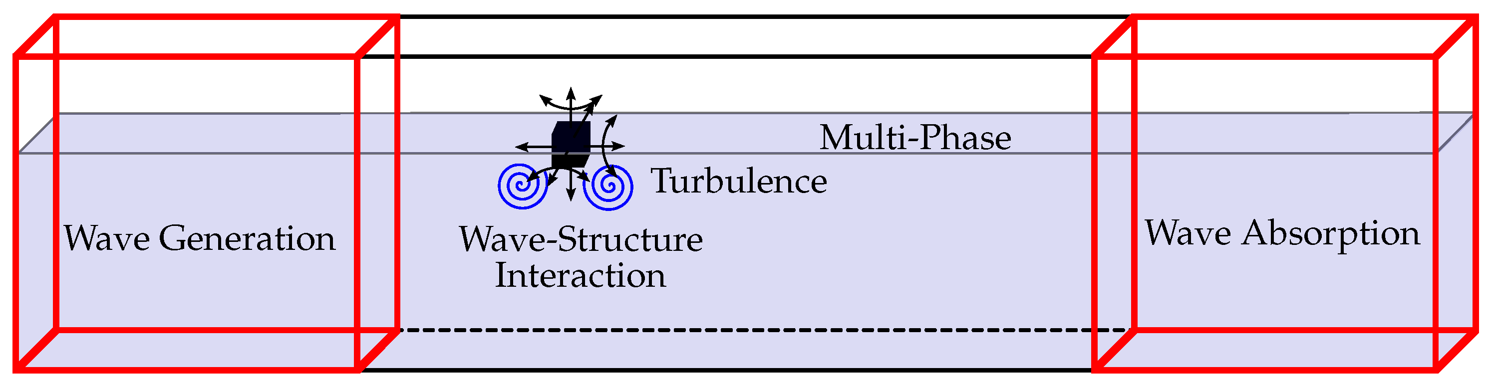
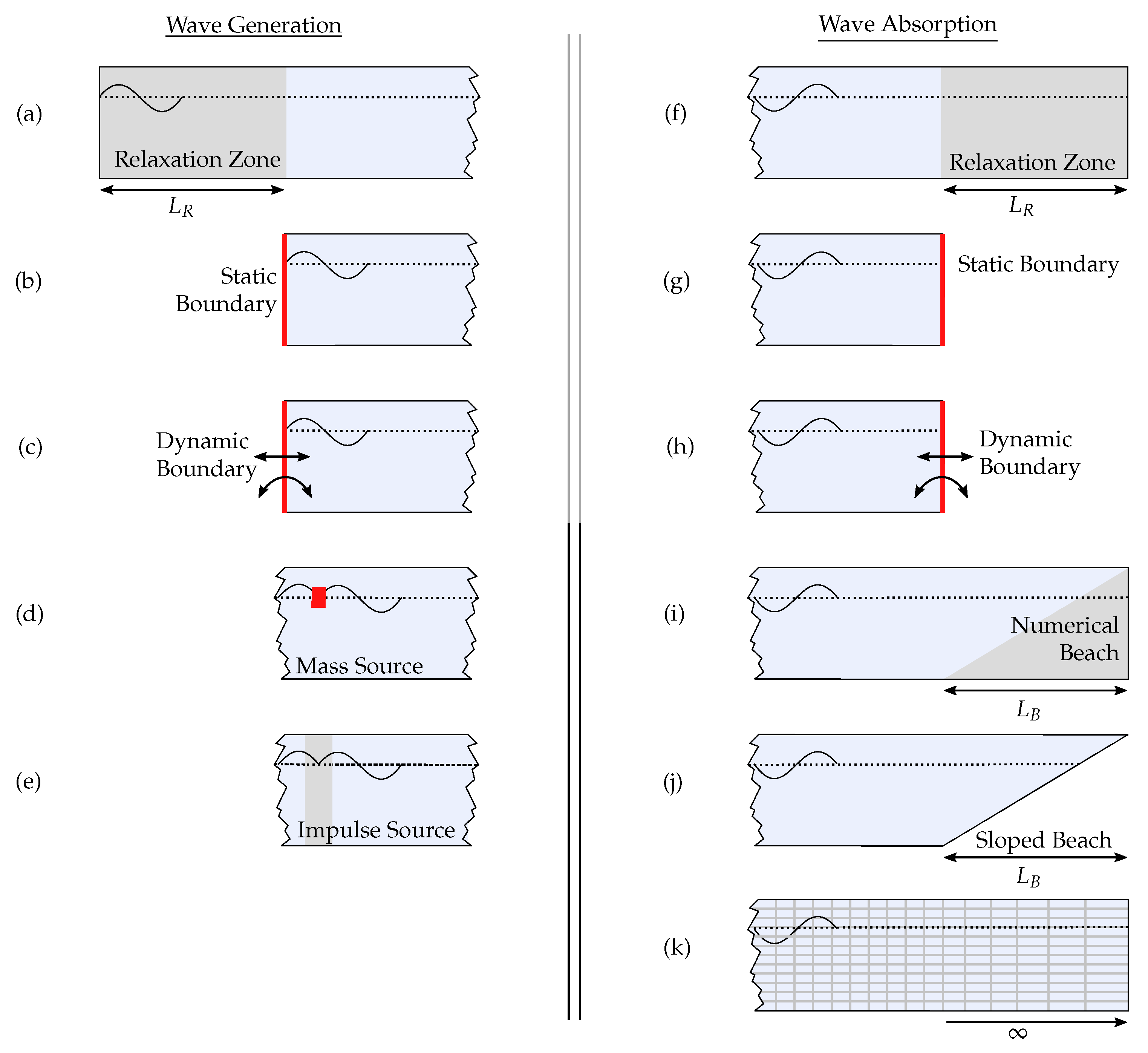
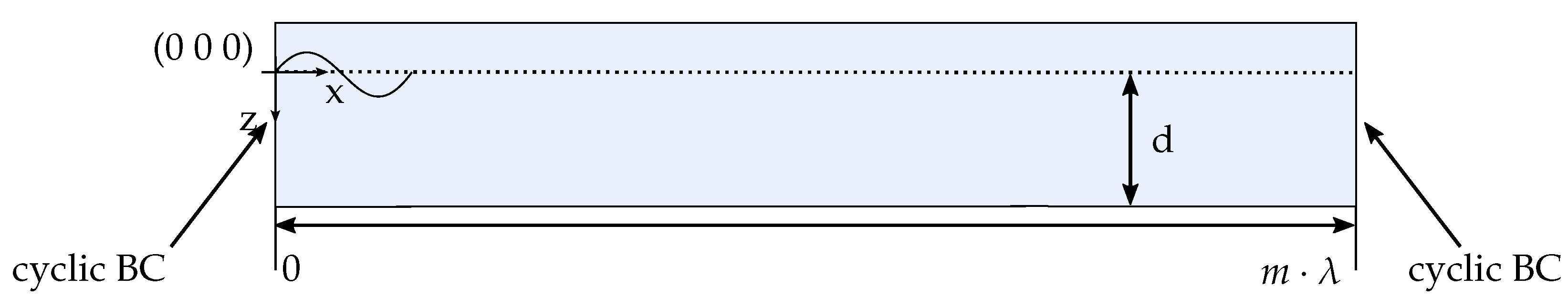
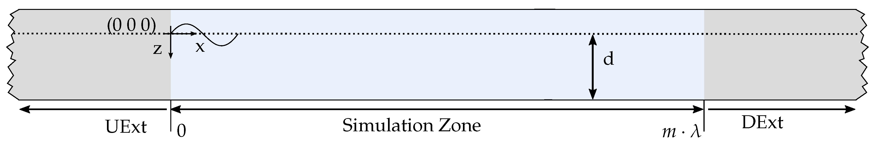
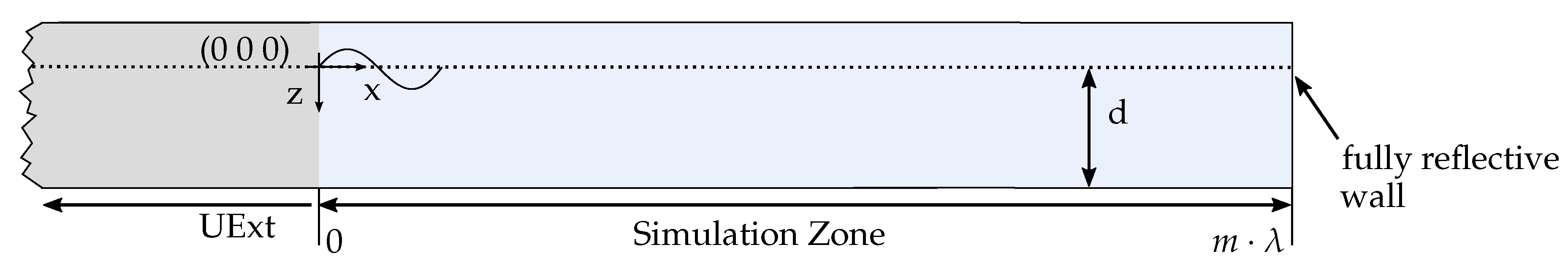
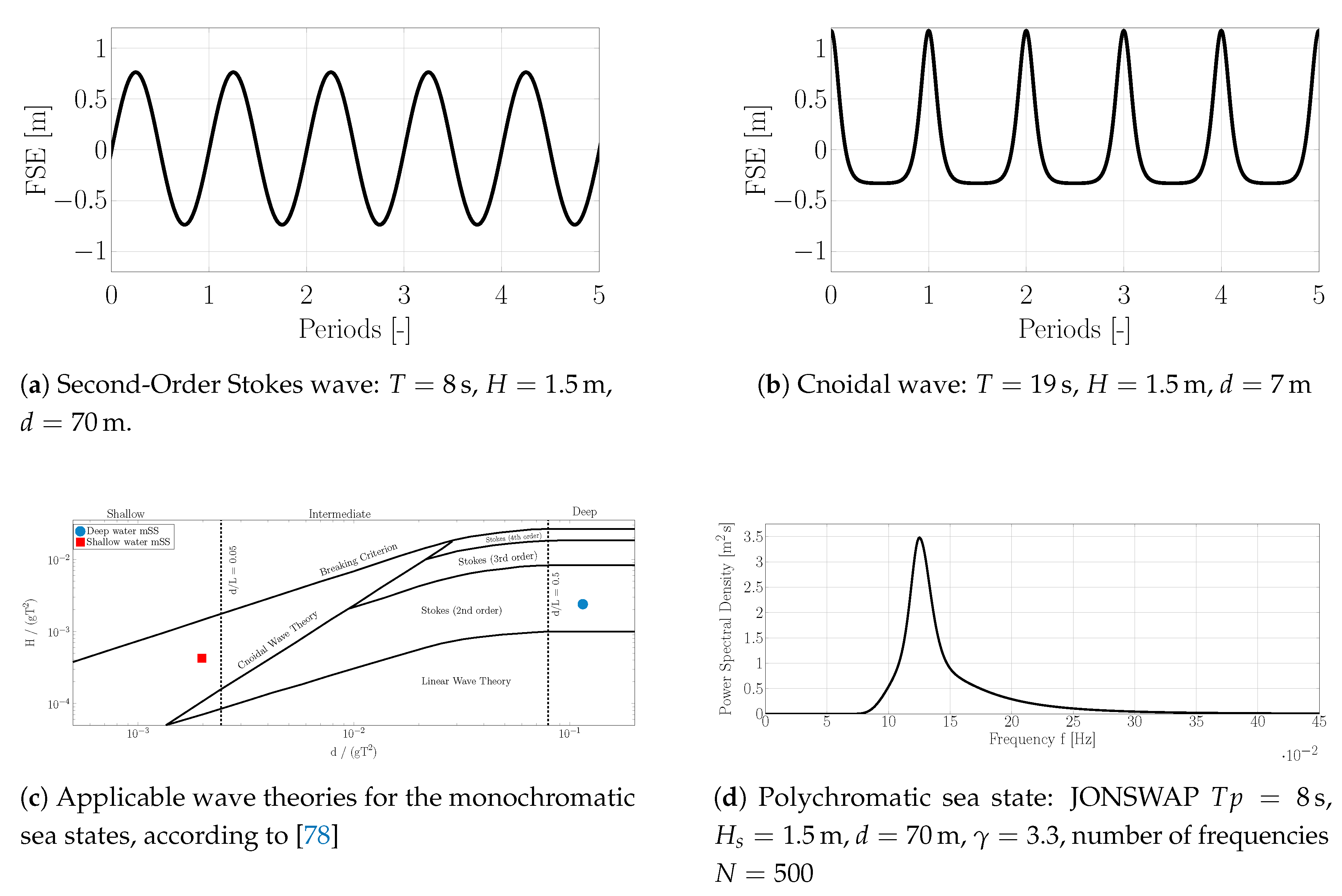
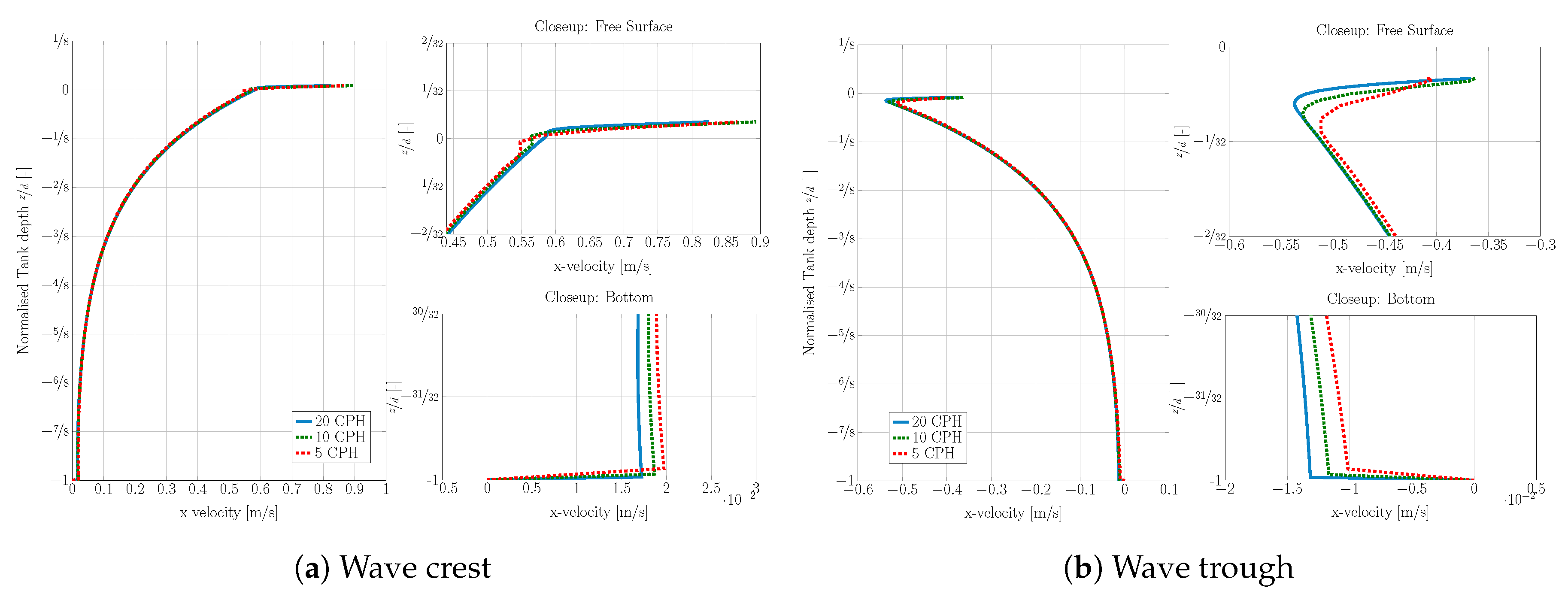
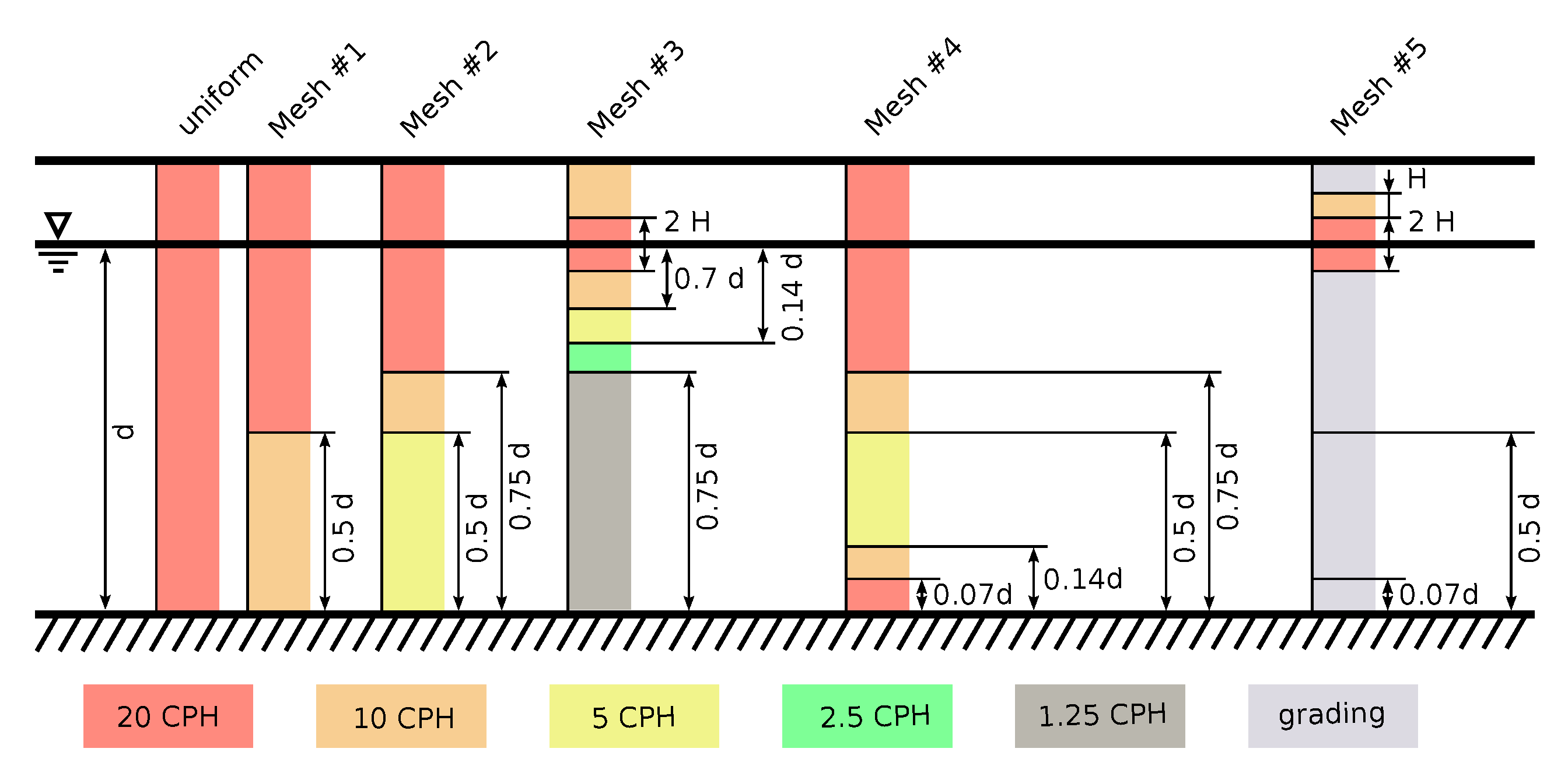
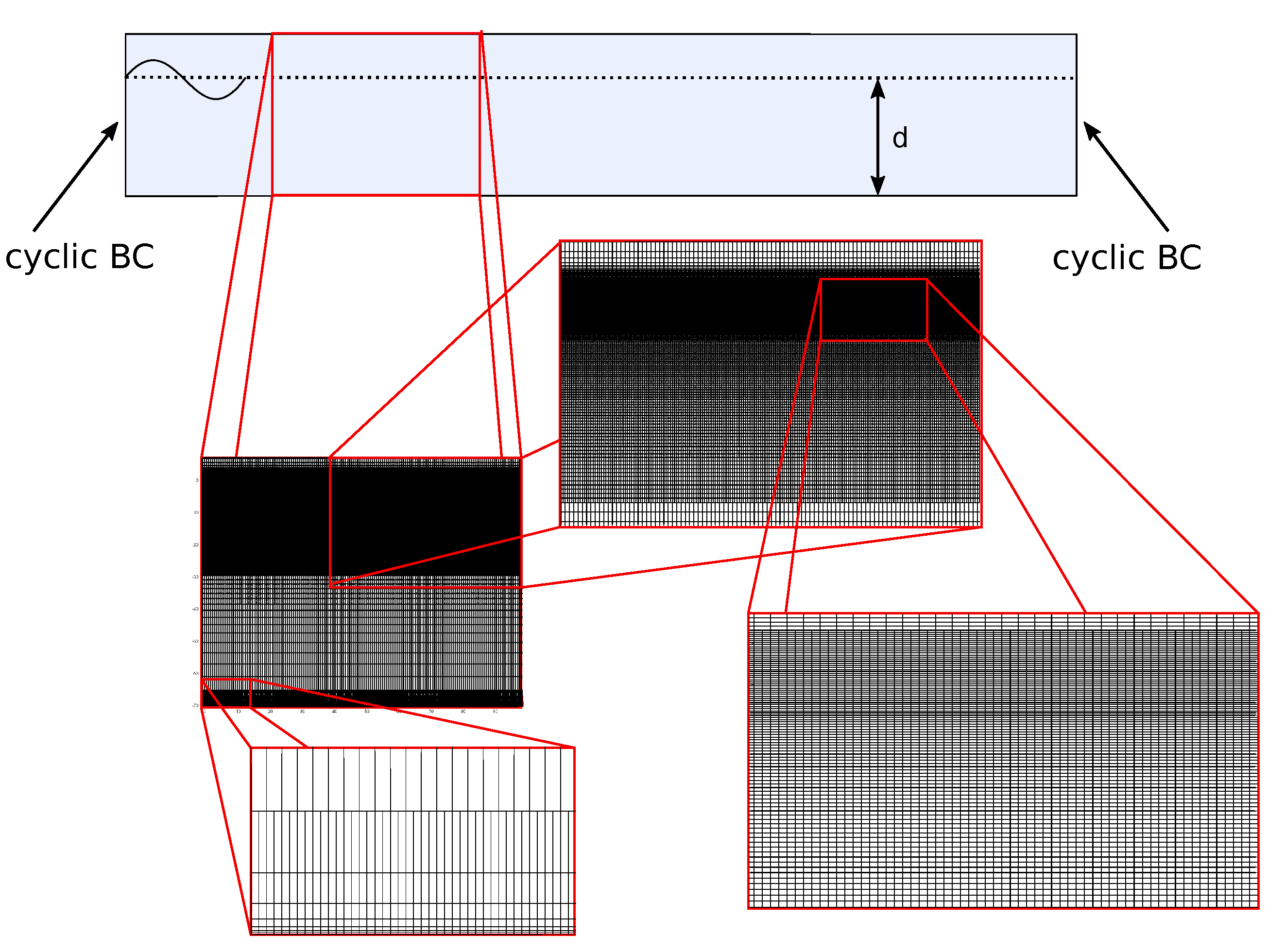
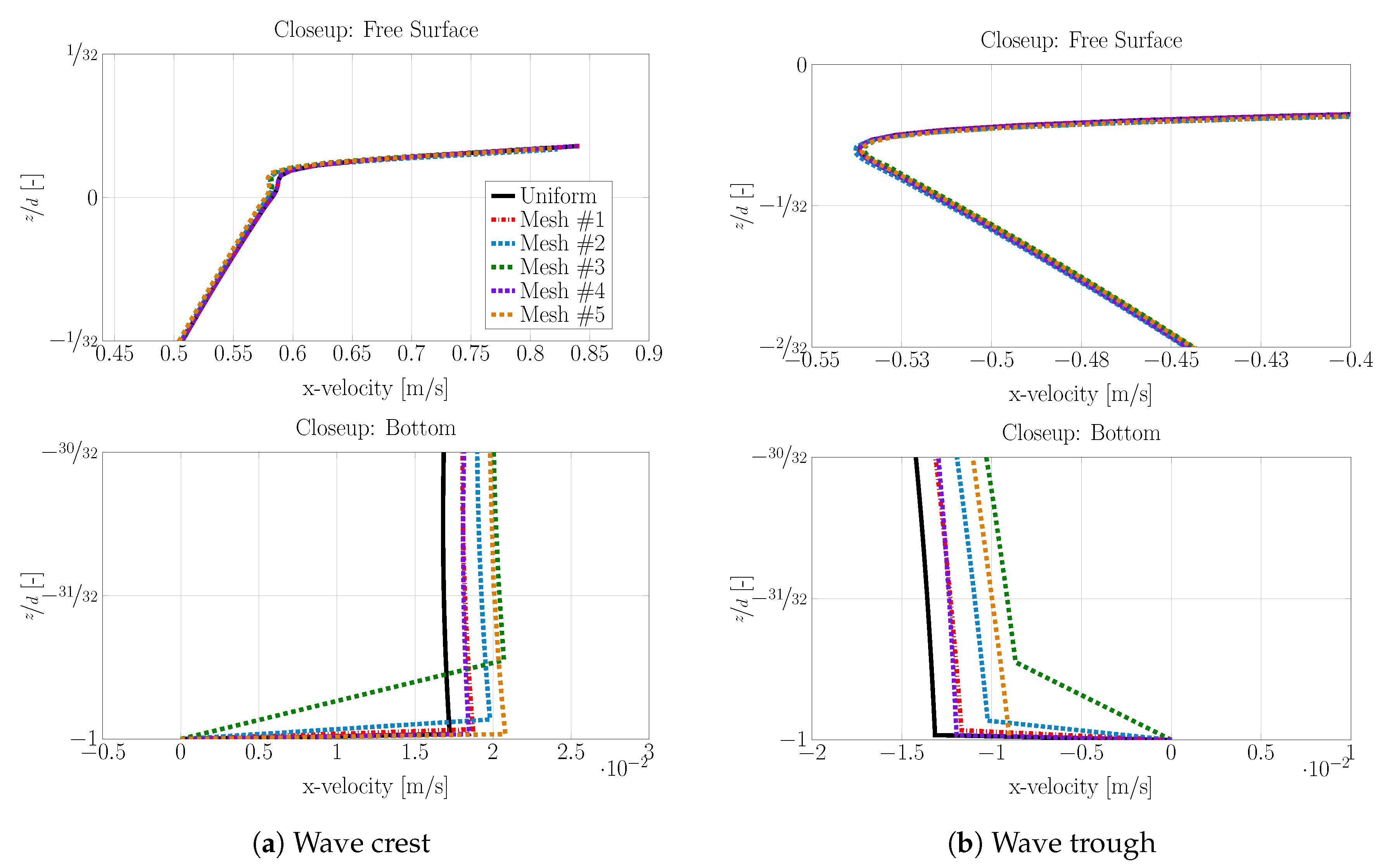
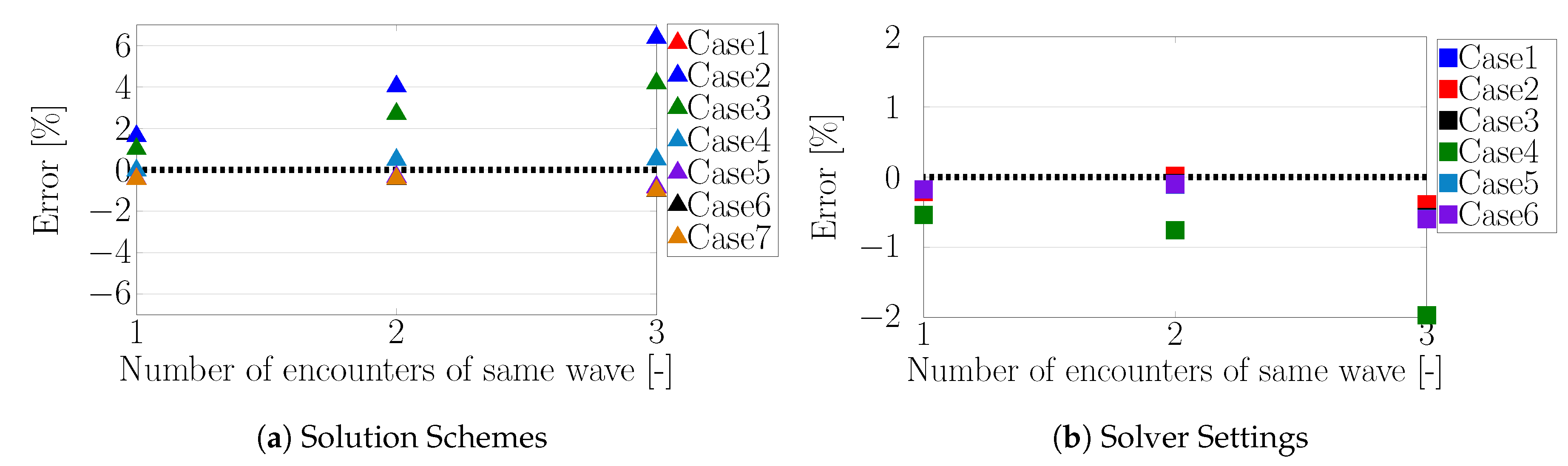
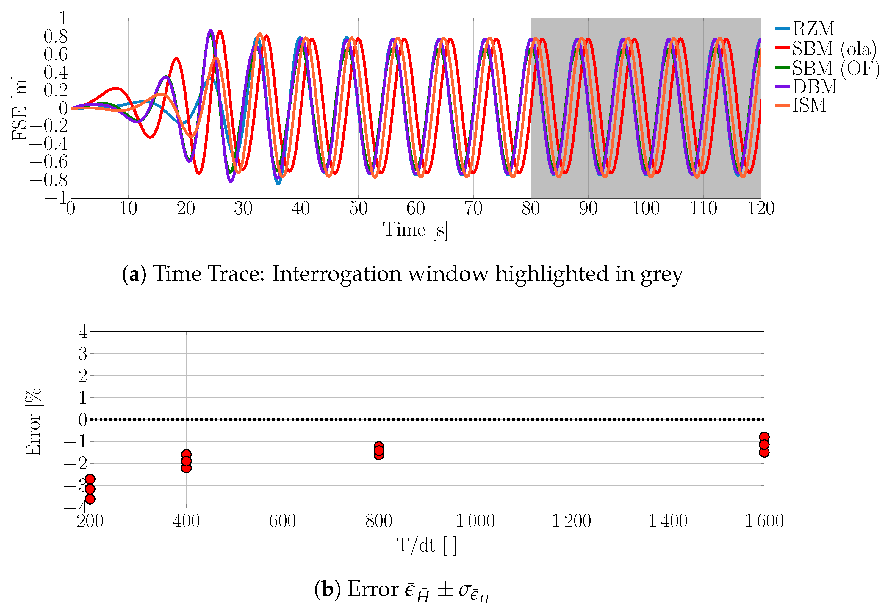
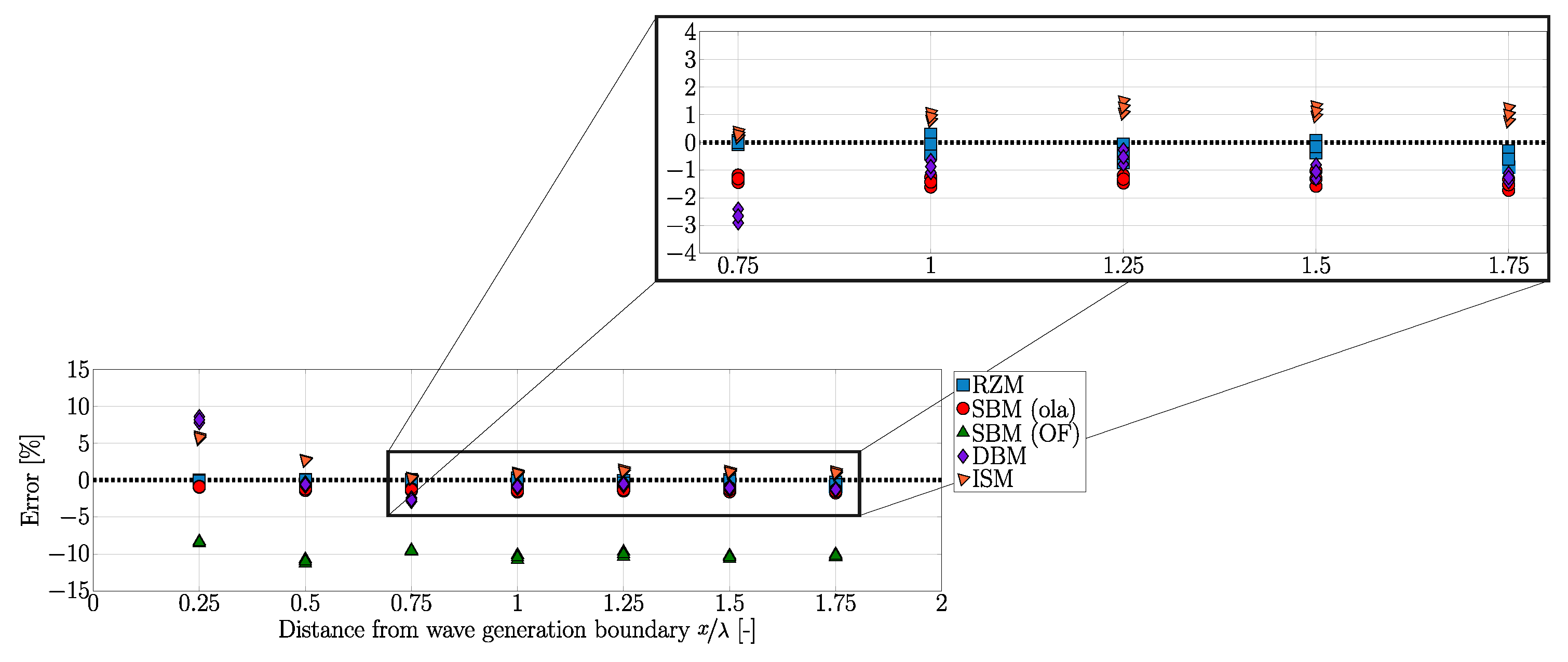
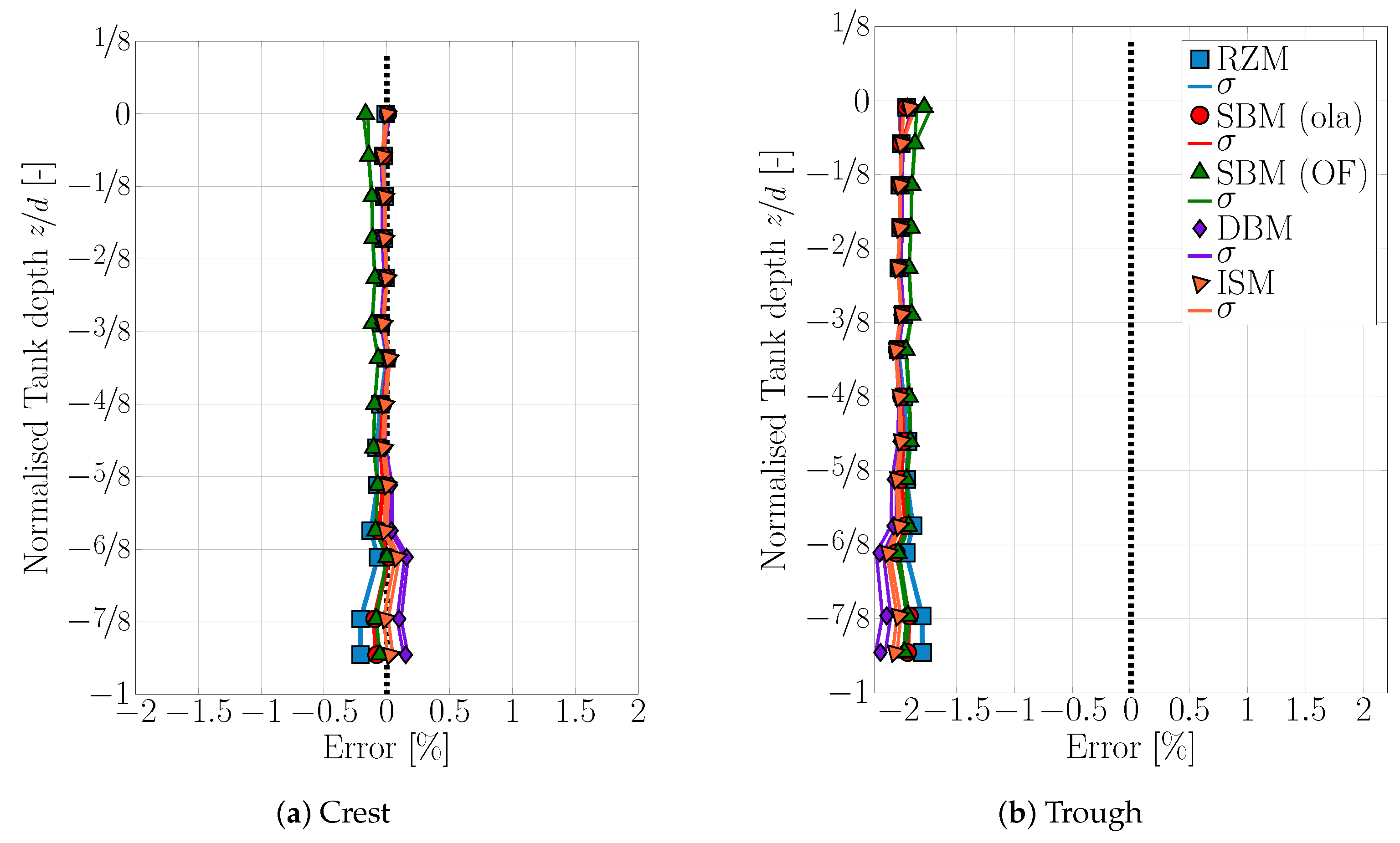
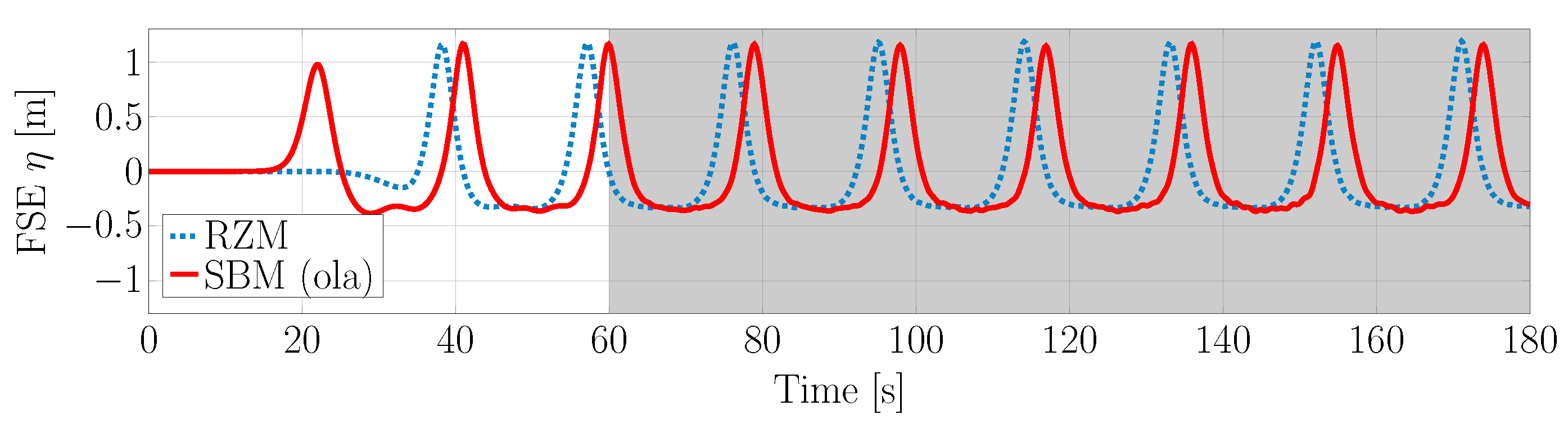
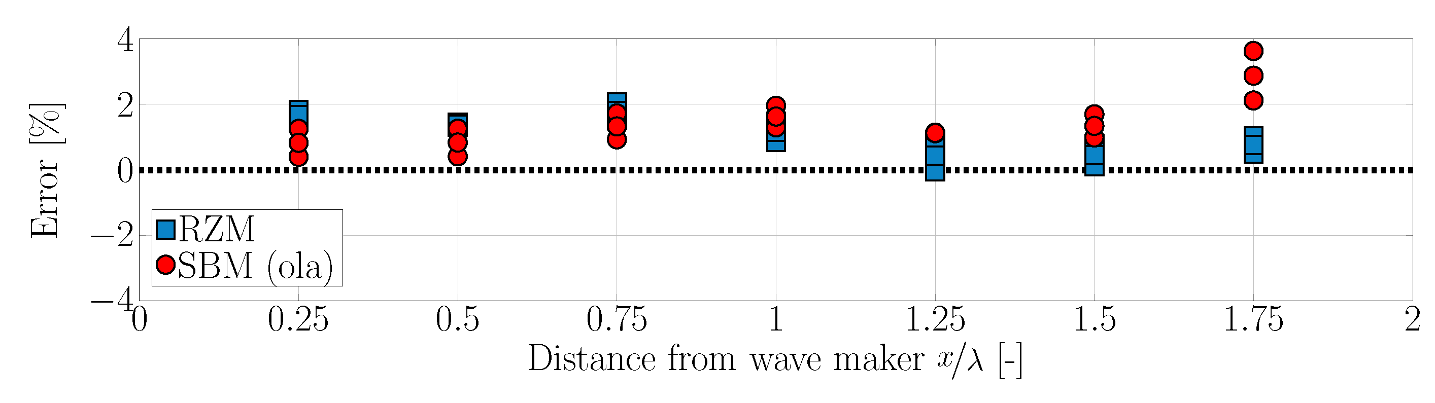
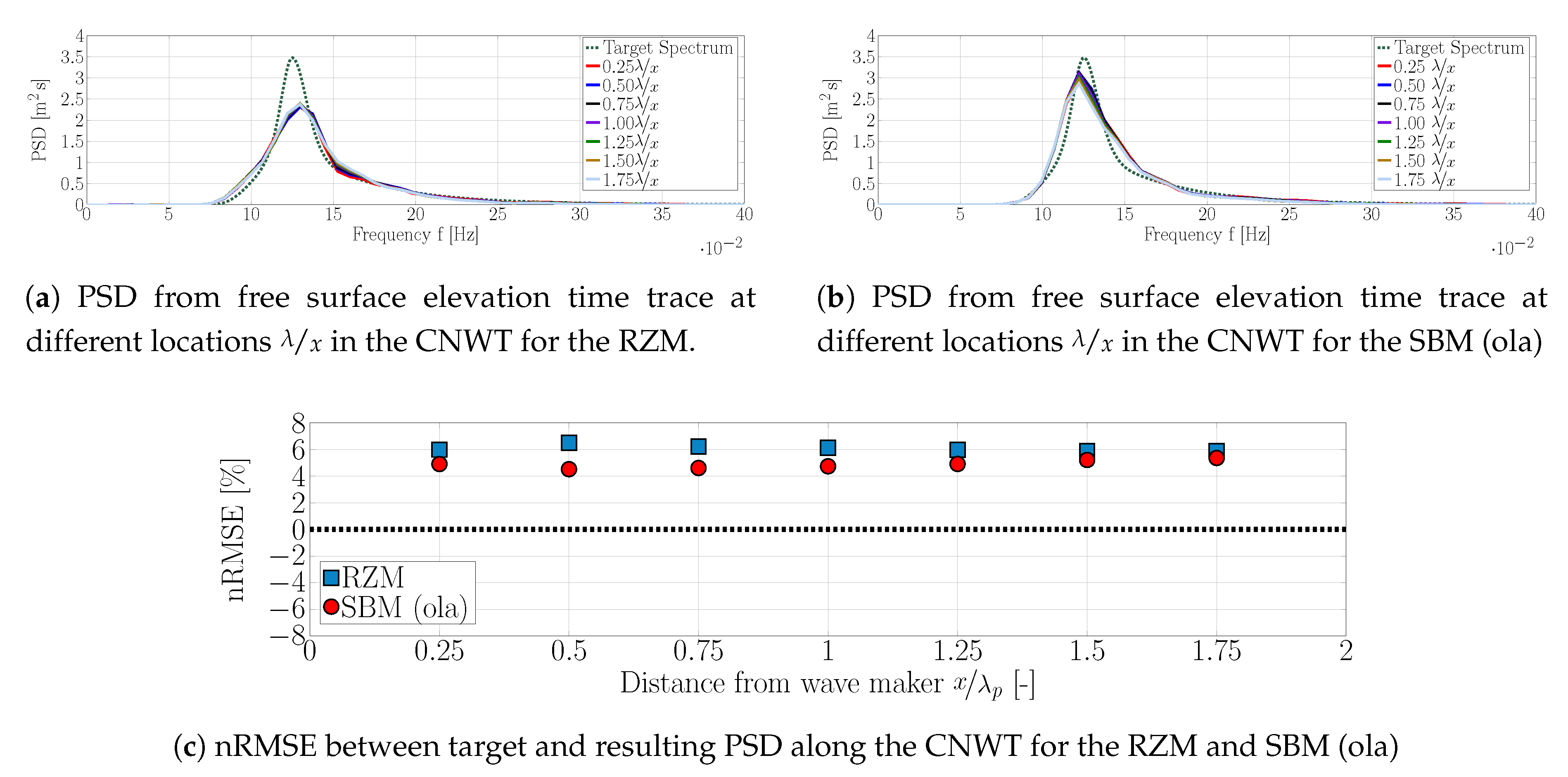
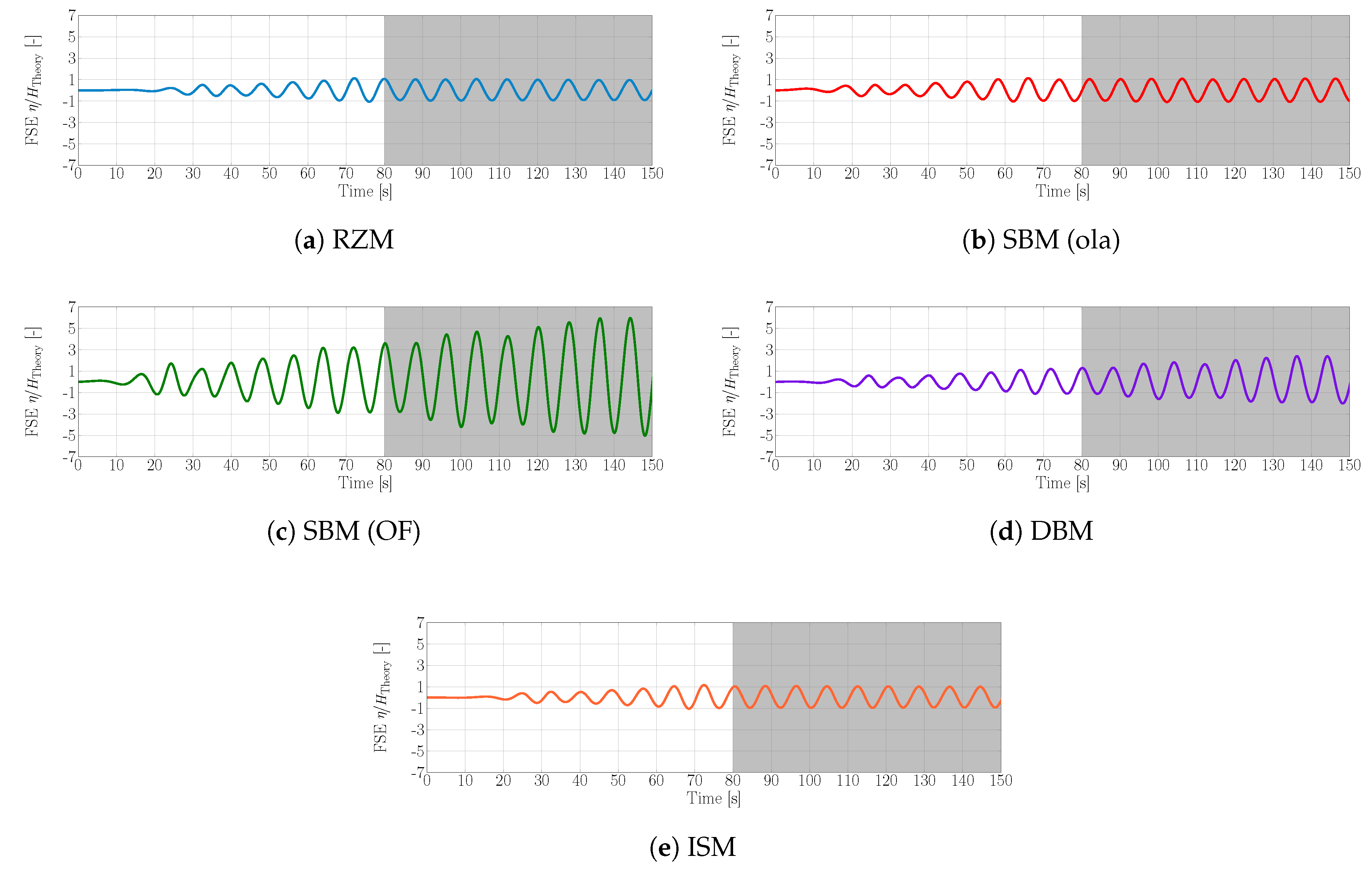
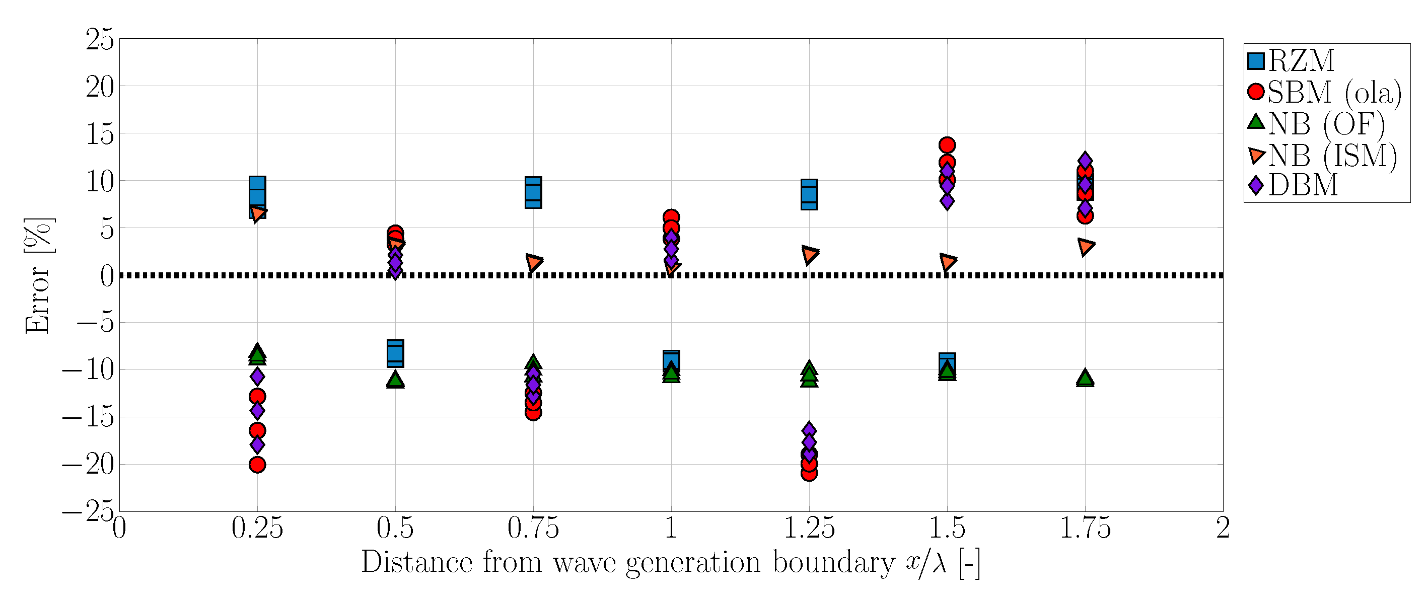
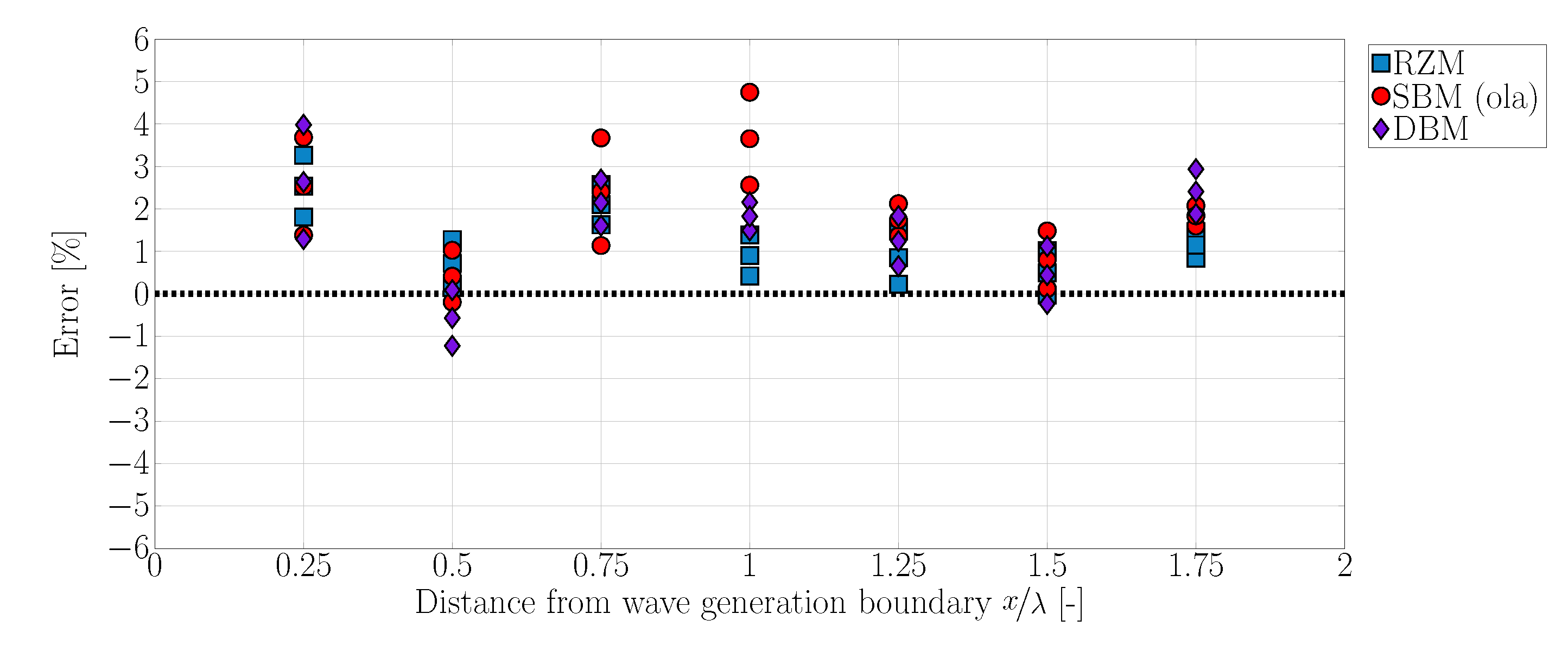
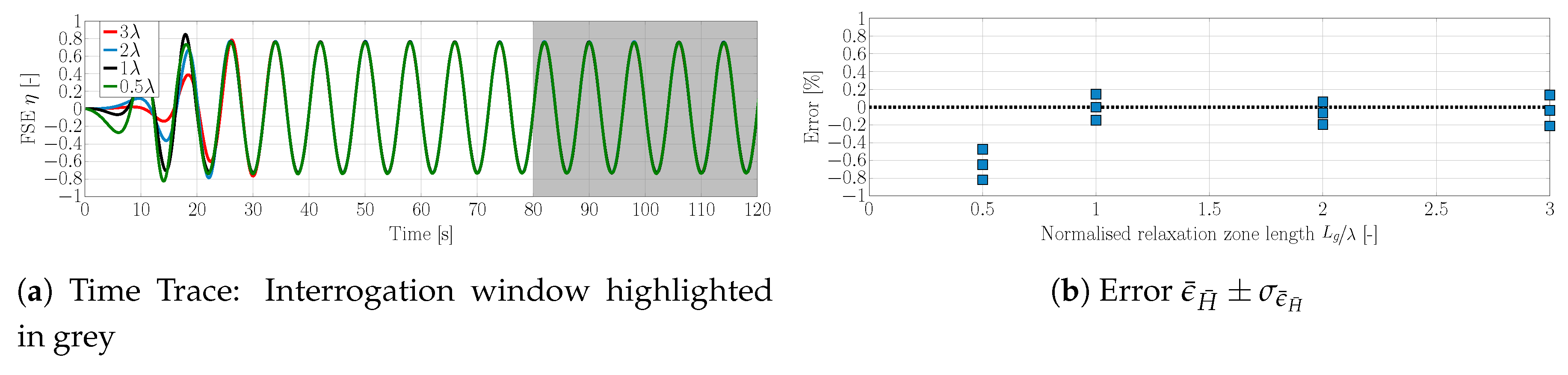
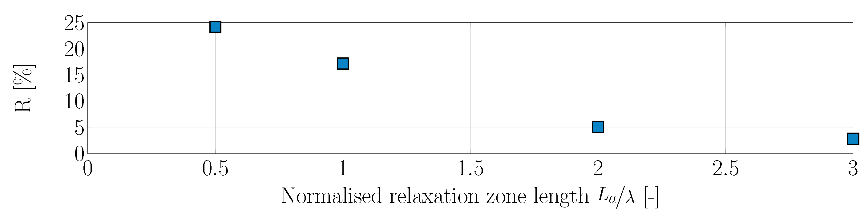
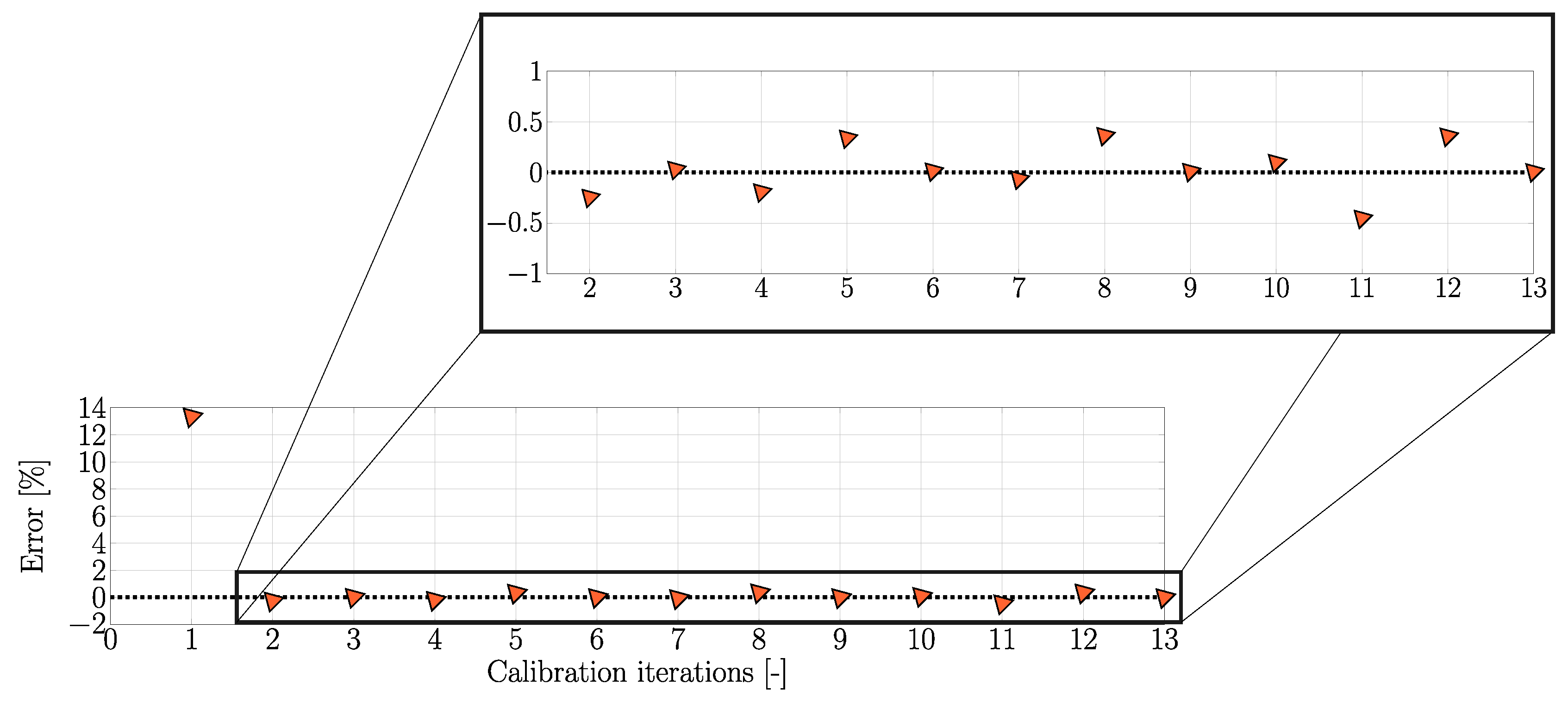
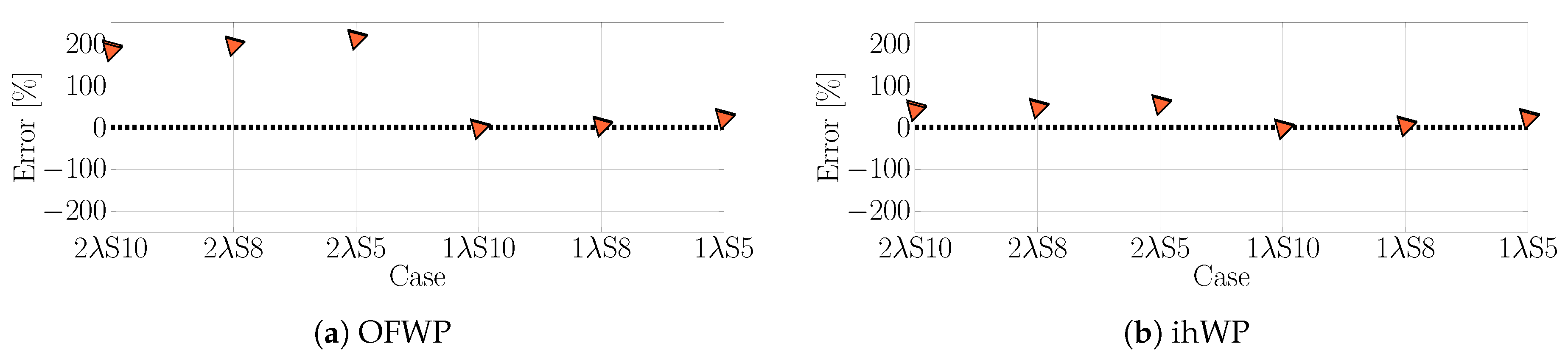
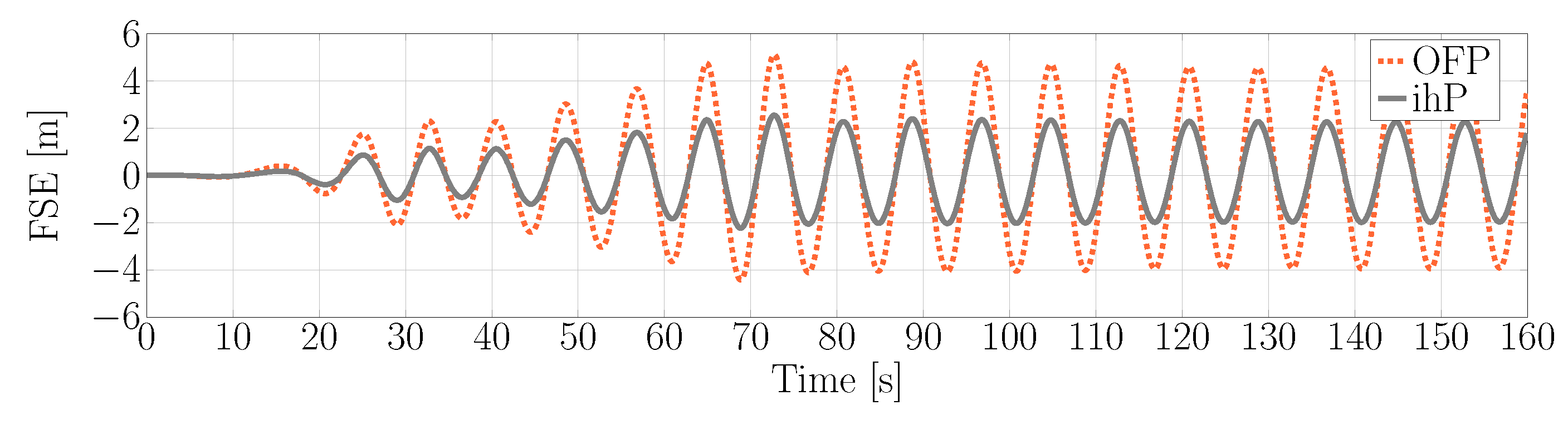
Table A1.
Convergence types based on the discrimination ratio .
| Convergence | |
|---|---|
| (i) Monotone Convergence | |
| (ii) Oscillatory Convergence | and |
| Divergence | |
| (i) Monotone Divergence | |
| (ii) Oscillatory Divergence | and |
Appendix B. Setup Details of the RZM
Appendix B.1. Calibration of the Generation Relaxation Zone
For the RZM, the optimal relaxation zone length at the wave generation boundary, , has to be determined. For that, simulations with varying were performed and the quality of the generated wave, by means of the relative deviation between measured and target wave height (Metric #3, Equation (15)), was monitored. For all simulations, the wave data were extracted at , so that any numerical wave damping could be neglected. The time step size for all simulations was kept constant at . For brevity, wave data were only extracted using the OFWP. Time traces of the free surface elevation , as well as the error , for the different lengths , are plotted in Figure A1a,b, respectively. Note that the interrogation window in which the zero up-crossing analysis was performed for the evaluation of is highlighted in grey in Figure A1a.
Figure A1.
Time traces of the free surface elevation (FSE) (a) and the error (b) for the different lengths .
Figure A1.
Time traces of the free surface elevation (FSE) (a) and the error (b) for the different lengths .

The results in Figure A1b indicate converged results for any , showing negligible errors in wave height. Since the relaxation zone length influences not only the accuracy of the wave generation but also the absorption capabilities at the wave generation boundary, results from the test case for wave absorption at the generator, i.e., Metric #6 (see Equation (22)), were considered. Time traces for and results for the error are shown in Figure A2a,b, respectively. Again, the interrogation window in which the zero up-crossing analysis was performed for the evaluation of is highlighted in grey in Figure A2a. Showing relatively small errors for , it is finally concluded that a relaxation zone length delivers satisfactory results. A more detailed discussion of the absorption capabilities at the wave generation boundary is presented in Section 5.5.
Figure A2.
Time traces of the FSE (a) and the error (b) for the different lengths .

Appendix B.2. Calibration of the Absorption Relaxation Zone
For the RZM, the optimal relaxation zone length at the wave absorption boundary has to be determined. For that, simulations with varying were performed and the reflection coefficient was monitored. Results are plotted in Figure A3.
Figure A3.
Reflection coefficient over different relaxation absorption zone lengths .

The results in Figure A3 indicate a decreasing reflection coefficient R, for increasing . No converged solution for the reflection coefficient was found for the tested range of . Given the correlation between an increased cell count (and run time) and increasing , the shortest possible relaxation zone length is desired. Since the improvement in wave absorption between and is relatively small compared to the improvement between and , a relaxation zone length of was chosen in all subsequent simulations.
Appendix C. Setup Details of the ISM and NB (ISM)
Appendix C.1. Calibration of the Impulse Source Input
The impulse source wave maker proposed by Schmitt et al. [48] uses an iterative calibration method to define the required time trace for the impulse source to generate the desired wave field. The calibration method shown by Schmitt et al. [48] is designed for polychromatic sea states and tested, for focused wave groups. In this study, the calibration method was adjusted to be able to generate nonlinear monochromatic waves.
From the target time trace, based on Stokes wave theory (see Figure 6a), the trough and crest peaks were defined as a reference. During the calibration procedure, the surface elevation was measured at a specific point in space (i.e., centre of the CNWT) and the resulting trough and crest free surface elevation values were extracted. The ratio between target and measured troughs and peaks was subsequently used to scale the impulse source input. Results of the wave height error over 13 calibration iterations are shown in Figure A4. Convergence of the error can be observed after the first calibration iteration, highlighting the efficiency of the calibration procedure. For all subsequent simulations of the deep water mSS, the impulse source input determined after three iterations was used.
Figure A4.
Wave height error over 13 calibration iterations.

As mentioned in Section 2, the ISM does not absorb waves travelling through the source, e.g., reflected waves from structures. Hence, a NB is required upstream of the NWM to prevent wave reflection from the upstream wall of the CNWT. In the implementation presented by Schmitt and Elsaesser [37], the NB has to be manually calibrated by tuning its length and the maximum damping factor S. For the calibration performed for this study, six different cases with two NB lengths (2 and 1) and three maximum damping factors () were tested. Figure A5 shows the results of this calibration by means of the standing wave error (Metric #6), based on free surface elevation data extracted with the OFWP (Figure A5a) and the ihWP (Figure A5b). The nomenclature for the different cases follows xSy, where x indicates the NB length and Sy the maximum damping factor.
Figure A5.
Error for different NB settings (length and damping factor) based on free surface elevation data extracted with the ihWP and OFWP.
Figure A5.
Error for different NB settings (length and damping factor) based on free surface elevation data extracted with the ihWP and OFWP.

The error plotted in Figure A5a shows a relatively large error of order for the cases with a NB length of . Based on results previously presented for the RZM (see Figure A2b), these errors appear to be too large. To check if these results are trustworthy, Metric #6 was applied to free surface elevation data sampled with the ihWP. As can be seen in Figure A5b, the error for the cases with a NB length of reduces considerably from to . This is further highlighted by the free surface elevation time trace plotted in Figure A6, extracted at the centre of the CNWT, using the OFWP and ihWP. This difference in measured free surface elevation, and subsequently in the determined error , must be caused by numerical errors in the numerical sampling procedure. Inspecting the mesh for the considered cases reveals that the centre of the CNWT exactly coincides with cell faces, which can cause such numerical errors. This result highlights the importance of cross checking the numerical results gained from the CNWT experiment.
The errors , for NB lengths of , stay unchanged for both WPs. The smallest error () can be found for the NB setting of 1S10, which is used for all subsequent simulations.
Figure A6.
Free surface elevation (FSE) time trace from simulations with a NB with length and damping factor S = 10 at the centre location of the CNWT extracted with the OFWP (dashed line) and ihWP (solid line).
Figure A6.
Free surface elevation (FSE) time trace from simulations with a NB with length and damping factor S = 10 at the centre location of the CNWT extracted with the OFWP (dashed line) and ihWP (solid line).

Appendix C.2. Calibration of the Down Wave NB
For the NB (ISM), a similar calibration study, as for the absorption zone length of the RZM, has to be performed, where six simulations with different NB settings were run. Varying the beach length from to , and the maximum damping factor S between and 10, the reflection coefficient R was evaluated. The resulting R value, for the different NB setting, are listed in Table A2. Ultimately, a NB length of , with a maximum damping factor S of 5, was chosen.
Table A2.
Reflection coefficients for different lengths and damping coefficients S of the NB (ISM).
| S 5 | S 8 | S 10 | |
|---|---|---|---|
| Beach Length | 4.5 | 6.1 | 6.9 |
| Beach Length | 2.0 | 2.7 | 3.1 |
Appendix D. Wave Height Error of the SBM (OF)
To investigate the source of the relatively large wave height error of the SBM (OF), the implementation of the free surface elevation was inspected. Generally, for second-order Stokes waves, the surface elevation is composed of the first-order, Airy, wave component and the second-order component, as shown in Equation (A6).
In Equation (A6), a denotes the wave amplitude, k is the wave number, is the substitute for , where d denotes the water depth. , where is the angular wave frequency.
The implemented equations for the second-order Stokes wave surface elevation can be extracted from the codes of the NWMs. These are shown below in Equations (A7)–(A9) for the SBM (ola), RZM and SBM (OF), respectively. For brevity, only the second-order part is shown in the equations.
Defining the term preceding in Equations (A7)–(A9) as a scaling factor, it can be seen that, for the deep water mSS, this scaling factor differs for by a factor of approximately 100, compared to and . This is an interesting result, since an under-estimation of the wave height can be observed in Figure 15 and Table 11. However, a larger scaling factor suggests over-estimation of the wave height.
For further investigation, a linear deep water wave, based on Airy wave theory, was simulated using the SBM (ola) and SBM (OF). Metric #3 was applied for the comparison. For the SBM (ola), an under-estimation of the wave height by was found, which falls in the same error range as for the second-order mSS. For the SBM (OF), an error of was found. Although this error is smaller than the error for the second-order mSS, it was still found to be relatively large compared to the error from the SBM (ola).
From this, it can be concluded that the error in the SBM (OF) stems from two sources. One relates to the second-order nature of the deep water mSS and a second source derives from inherent modelling inaccuracies, unrelated to the considered wave. A more detailed analysis of the error in the SBM (OF) should be part of future work.
References
- Tanizawa, K. The state of the art on numerical wave tank. In Proceedings of the 4th Osaka Colloquium on Seakeeping Performance of Ships 2000, Osaka, Japan, 17–21 October 2000; pp. 95–114. [Google Scholar]
- Schmitt, P.; Doherty, K.; Clabby, D.; Whittaker, T. The opportunities and limitations of using CFD in the development of wave energy converters. In Proceedings of the International Conference on Marine & Offshore Renewable Energy, London, UK, 26–27 September 2012. [Google Scholar]
- Penalba, M.; Giorgi, G.; Ringwood, J.V. Mathematical Modelling of Wave Energy Converters: A Review of Nonlinear Approaches. Renew. Sustain. Energy Rev. 2017, 78, 1188–1207. [Google Scholar] [CrossRef]
- Windt, C.; Davidson, J.; Ringwood, J. High-fidelity numerical modelling of ocean wave energy systems: A review of CFD-based numerical wave tanks. Renew. Sustain. Energy Rev. 2018, 93, 610–630. [Google Scholar] [CrossRef]
- Kim, J.W.; Jang, H.; Baquet, A.; O’Sullivan, J.; Lee, S.; Kim, B.; Jasak, H. Technical and economic readiness review of CFD-Based numerical wave basin for offshore floater design. In Proceedings of the Offshore Technology Conference, Houston, TX, USA, 5 May 2016. [Google Scholar]
- Day, A.H.; Babarit, A.; Fontaine, A.; He, Y.P.; Karaskowski, M.; Murai, M.; Penesis, I.; Salvatore, F.; Shin, H.K. Hydrodynamic modelling of marine renewable energy devices: A state of the art review. Ocean Eng. 2015, 108, 46–69. [Google Scholar] [CrossRef]
- Wolgamot, H.A.; Fitzgerald, C.J. Nonlinear hydrodynamic and real fluid effects on wave energy converters. Proc. Inst. Mech. Eng. Part A J. Power Energy 2015, 229, 772–794. [Google Scholar] [CrossRef]
- Ortloff, C.; Krafft, M. Numerical Test Tank: Simulation of Ocean Engineering Problems by Computational Fluid Dynamics. In Proceedings of the Offshore Technology Conference, Houston, TX, USA, 5–8 May 1997; pp. 23–31. [Google Scholar]
- Higuera, P.; Lara, J.L.; Losada, I.J. Realistic wave generation and active wave absorption for Navier–Stokes models application to OpenFOAM. Coast. Eng. 2013, 71, 102–118. [Google Scholar] [CrossRef]
- Clauss, G.F.; Schmittner, C.E.; Stuck, R. Numerical wave tank: Simulation of extreme waves for the investigation of structural responses. In Proceedings of the ASME 2005 24th International Conference on Offshore Mechanics and Arctic Engineering, Halkidiki, Greece, 12–17 June 2005; pp. 785–792. [Google Scholar]
- Westphalen, J.; Greaves, D.; Williams, C.; Hunt-Raby, A.; Zang, J. Focused waves and wave–structure interaction in a numerical wave tank. Ocean Eng. 2012, 45, 9–21. [Google Scholar] [CrossRef]
- Lu, X.; Kumar, P.; Bahuguni, A.; Wu, Y. A CFD study of focused extreme wave impact on decks of offshore structures. In Proceedings of the ASME 2014 33rd International Conference on Ocean, Offshore and Arctic Engineering, San Francisco, CA, USA, 8–13 June 2014. [Google Scholar]
- Chella, M.A.; Bihs, H.; Myrhaug, D. Characteristics and profile asymmetry properties of waves breaking over an impermeable submerged reef. Coast. Eng. 2015, 100, 26–36. [Google Scholar] [CrossRef]
- Chen, H.; Christensen, E.D. Numerical simulation of wave interaction with moving net structures. In Proceedings of the ASME 2015 34th International Conference on Ocean, Offshore and Arctic Engineering, St. John’s, NL, Canada, 31 May–June 5 2015. [Google Scholar]
- Zhu, R.; Miao, G.; Lin, Z. Numerical research on FPSOs with green water occurrence. J. Ship Res. 2009, 53, 7–18. [Google Scholar]
- Cavallaro, L.; Dentale, F.; Donnarumma, G.; Foti, E.; Musumeci, R.E.; Carratelli, E.P. Rubble mound breakwater overtopping: Estimation of the reliability of a 3D numerical simulation. Coast. Eng. Proc. 2012, 1. [Google Scholar] [CrossRef]
- Ahmad, N.; Bihs, H.; Kamath, A.; Arntsen, Ø.A. Three-dimensional CFD modeling of wave scour around side-by-side and triangular arrangement of piles with REEF3D. Procedia Eng. 2015, 116, 683–690. [Google Scholar] [CrossRef]
- Liu, Y.; Wan, D. Numerical simulation of motion response of an offshore observation platform in waves. J. Mar. Sci. Appl. 2013, 12, 89–97. [Google Scholar] [CrossRef]
- Irkal, M.A.; Nallayarasu, S.; Bhattacharyya, S. CFD approach to roll damping of ship with bilge keel with experimental validation. Appl. Ocean Res. 2016, 55, 1–17. [Google Scholar] [CrossRef]
- Wang, J.; Zou, L.; Wan, D. CFD simulations of free running ship under course keeping control. Ocean Eng. 2017, 141, 450–464. [Google Scholar] [CrossRef]
- Zwart, P.J.; Godin, P.G.; Penrose, J.; Rhee, S.H. Simulation of unsteady free-surface flow around a ship hull using a fully coupled multi-phase flow method. J. Mar. Sci. Technol. 2008, 13, 346–355. [Google Scholar] [CrossRef]
- Hu, X.Z.; Liu, S.J. Two-dimensional numerical wave tank simulation for deployment of seafloor mining system. Mar. Georesour. Geotechnol. 2014, 32, 293–306. [Google Scholar] [CrossRef]
- Hirt, C.W.; Nichols, B.D. Volume of Fluid (VOF) Method for the Dynamics of Free Boundaries. J. Comput. Phys. 1981, 39, 201–225. [Google Scholar] [CrossRef]
- Berberović, E.; van Hinsberg, N.P.; Jakirlić, S.; Roisman, I.V.; Tropea, C. Drop impact onto a liquid layer of finite thickness: Dynamics of the cavity evolution. Phys. Rev. E 2009, 79, 036306-1–036306-15 . [Google Scholar] [CrossRef] [PubMed]
- Devolder, B.; Troch, P.; Rauwoens, P. Performance of a buoyancy-modified k-ω and k-ω SST turbulence model for simulating wave breaking under regular waves using OpenFOAM®. Coast. Eng. 2018, 138, 49–65. [Google Scholar] [CrossRef]
- Vukčević, V.; Jasak, H.; Gatin, I. Implementation of the Ghost Fluid Method for free surface flows in polyhedral Finite Volume framework. Comput. Fluids 2017, 153, 1–19. [Google Scholar] [CrossRef]
- Roenby, J.; Bredmose, H.; Jasak, H. IsoAdvector: Geometric VOF on general meshes. In Proceedings of the 11th OpenFOAM Workshop, Exeter, UK, 24–27 July 2017. [Google Scholar]
- Gatin, I.; Vladimir, N.; Malenica, Š.; Jasak, H. Green sea loads in irregular waves with Finite Volume method. Ocean Eng. 2019, 171, 554–564. [Google Scholar] [CrossRef]
- Palm, J.; Eskilsson, C.; Bergdahl, L.; Bensow, R. Assessment of scale effects, viscous forces and induced drag on a point-absorbing wave energy converter by CFD simulations. J. Mar. Sci. Eng. 2018, 6, 124. [Google Scholar] [CrossRef]
- Westphalen, J.; Greaves, D.M.; Raby, A.; Hu, Z.Z.; Causon, D.M.; Mingham, C.G.; Omidvar, P.; Stansby, P.K.; Rogers, B.D. Investigation of wave-structure interaction using state of the art CFD techniques. Open J. Fluid Dyn. 2014, 4, 18–43. [Google Scholar] [CrossRef]
- Xu, L.; Baglietto, E.; Brizzolara, S. Extending the applicability of RANS turbulence closures to the simulation of transitional flow around hydrofoils at low Reynolds number. Ocean Eng. 2018, 164, 1–12. [Google Scholar] [CrossRef]
- Stansby, P.; Gu, H.; Moreno, E.C.; Stallard, T. Drag minimisation for high capture width with three float wave energy converter M4. In Proceedings of the 11th European Wave and Tidal Energy Conference, Nantes, France, 6–11 September 2015; pp. 6–11. [Google Scholar]
- del Jesus, M.; Lara, J.L.; Losada, I.J. Three-dimensional interaction of waves and porous coastal structures: Part I: Numerical model formulation. Coast. Eng. 2012, 64, 57–72. [Google Scholar] [CrossRef]
- Jacobsen, N.; Fuhrmann, D.R.; Fredsø, J. A wave generation toolbox for the open-source CFD library: OpenFoam(R). Int. J. Numer. Methods Fluids 2012, 70, 1073–1088. [Google Scholar] [CrossRef]
- Higuera, P.; Lara, J.L.; Losada, I.J. Simulating coastal engineering processes with OpenFOAM®. Coast. Eng. 2013, 71, 119–134. [Google Scholar] [CrossRef]
- Windt, C.; Davidson, J.; Schmitt, P.; Ringwood, J.V. Development of an impulse source-based wave-current interaction (WCI) model. In Proceedings of the 7th European Conference on Computational Fluid Dynamics, Glasgow, UK, 11–15 June 2018; pp. 1406–1416. [Google Scholar]
- Schmitt, P.; Elsaesser, B. A review of wave makers for 3D numerical simulations. In Proceedings of the MARINE 2015—Computational Methods in Marine Engineering VI, Rome, Italy, 15–17 June 2015; pp. 437–446. [Google Scholar]
- Windt, C.; Davidson, J.; Schmitt, P.; Ringwood, J.V. Assessment of Numerical Wave Makers. In Proceedings of the 12th European Wave and Tidal Energy Conference, Cork, Ireland, 27 August–1 September 2017; pp. 707-1–707-10. [Google Scholar]
- Miquel, A.; Kamath, A.; Chella, M.; Archetti, R.; Bihs, H. Analysis of Different Methods for Wave Generation and Absorption ina CFD-Based Numerical Wave Tank. J. Mar. Sci. Eng. 2018, 6, 73. [Google Scholar] [CrossRef]
- Afshar, M.A. Numerical Wave Generation in OpenFOAM. Master’s Thesis, Department of Shipping and Marine Technology, Chalmers University of Technology, Göteborg, Sweden, 2010. [Google Scholar]
- Jasak, H.; Vukčević, V.; Gatin, I. Numerical Simulation of Wave Loading on Static Offshore Structures. In Springer Tracts in Mechanical Engineering; Springer International Publishing: Berlin, Germany, 2015; pp. 95–105. [Google Scholar]
- Higuera, P. Application of Computational Fluid Dynamics to Wave Action on Structures. Ph.D. Thesis, School of Civil Engineering, University of Cantabria, Cantabria, Spain, 2015. [Google Scholar]
- Lin, P.; Liu, P.L.F. Internal wave-maker for Navier-Stokes equations models. J. Waterw. Port Coast. Ocean Eng. 1999, 125, 207–215. [Google Scholar] [CrossRef]
- Peric, R.; Abdel-Maksoud, M. Generation of free-surface waves by localized source terms in the continuity equation. Ocean Eng. 2015, 109, 567–579. [Google Scholar] [CrossRef]
- Choi, J.; Yoon, S.B. Numerical simulations using momentum source wave-maker applied to RANS equation model. Coast. Eng. 2009, 56, 1043–1060. [Google Scholar] [CrossRef]
- Ha, T.; Lin, P.; Cho, Y.S. Generation of 3D regular and irregular waves using Navier-Stokes equations model with an internal wave maker. Coast. Eng. 2013, 76, 55–67. [Google Scholar] [CrossRef]
- Saincher, S.; Banerjee, J. On wave damping occurring during source-based generation of steep waves in deep and near-shallow water. Ocean Eng. 2017, 135, 98–116. [Google Scholar] [CrossRef]
- Schmitt, P.; Windt, C.; Davidson, J.; Ringwood, J.; Whittaker, T. The efficient application of an Impulse Source wave maker to CFD simulations. J. Mar. Sci. Eng. 2019. submitted. [Google Scholar]
- Chen, L.; Zang, J.; Hillis, A.; Morgan, G.; Plummer, A. Numerical investigation of wave-structure interaction using OpenFOAM. Ocean Eng. 2014, 88, 91–109. [Google Scholar] [CrossRef]
- Finnegan, W.; Goggins, J. Numerical simulation of linear water waves and wave–structure interaction. Ocean Eng. 2012, 43, 23–31. [Google Scholar] [CrossRef]
- López, I.; Pereiras, B.; Castro, F.; Iglesias, G. Optimisation of turbine-induced damping for an OWC wave energy converter using a RANS–VOF numerical model. Appl. Energy 2014, 127, 105–114. [Google Scholar] [CrossRef]
- Chen, Z.; Singh, P.M.; Choi, Y.D. Structural Analysis on the Arm and Floater Structure of a Wave Energy Converter. KSFM J. Fluid Mach. 2015, 18, 5–11. [Google Scholar] [CrossRef]
- Davidson, J.; Cathelain, M.; Guillemet, L.; Le Huec, T.; Ringwood, J. Implementation of an OpenFOAM Numerical Wave Tank for Wave Energy Experiments. In Proceedings of the 11th European Wave and Tidal Energy Conference, Nantes, Nantes, France, 6–11 September 2015; pp. 9B1-1-1–9B1-1-10. [Google Scholar]
- Schäffer, H.A.; Klopman, G. Review of Multidirectional Active Wave Absorption Methods. J. Waterw. Port Coast. Ocean Eng. 2000, 126, 88–97. [Google Scholar] [CrossRef]
- olaFlow. Available online: https://sites.google.com/view/olaflowcfd/blog/active-wave-absorption-enhancements-in-olaflow (accessed on 25 January 2019).
- Galvin, C. Wave-Height Prediction for Wave Generatros in Shallow Water; Technical Report; US Army Coastal Engineering Research Center: Vicksburg, MS, USA, 1964. [Google Scholar]
- Hughes, S.A. Physical Models and Laboratory Techniques in Coastal Engineering; World Scientific: Singapore, 1993; Volume 7. [Google Scholar]
- Clement, A. Coupling of Two Absorbing Boundary Conditions for 2D Time-Domain Simulations of Free Surface Gravity Waves. J. Comput. Phys. 1996, 126, 139–151. [Google Scholar] [CrossRef]
- Chen, L. Modelling of Marine Renewable Energy. Ph.D. Thesis, Department of Architecture and Civil Engineering, University of Bath, Bath, UK, 2015. [Google Scholar]
- Anbarsooz, M.; Passandideh-Fard, M.; Moghiman, M. Numerical simulation of a submerged cylindrical wave energy converter. Renew. Energy 2014, 64, 132–143. [Google Scholar] [CrossRef]
- Scarpetta, F.; Martina, G.; Torresi, M.; Camporeale, S.M. CFD analysis of the wave interaction with both a submerged impermeable breakwater and one embedding an OWC device. In Proceedings of the 11th European Wave and Tidal Energy Conference, Nantes, France, 6–11 September 2015; pp. 10B2-5-1–10B2-5-6. [Google Scholar]
- Bhinder, M.A.; Mingham, C.G.; Causon, D.M.; Rahmati, M.T.; Aggidis, G.A.; Chaplin, R. Numerical and Experimental Study of a Surging Point Absorber Wave Energy Converter. In Proceedings of the 8th European Wave and Tidal Energy Conference, Uppsala, Sweden, 7–10 September 2009. [Google Scholar]
- Westphalen, J.; Greaves, D.; Williams, C.; Taylor, P.; Causon, D.; Mingham, C.; Hu, Z.; Stansby, P.; Rogers, B.; Omidvar, P. Extreme Wave Loading on Offshore Wave Energy Devices using CFD: A Hierarchical Team Approach. In Proceedings of the 8th European Wave and Tidal Energy Conference 2009, Uppsala, Sweden, 7–10 September 2009. [Google Scholar]
- Davidson, J.; Giorgi, S.; Ringwood, J.V. Linear parametric hydrodynamic models for ocean wave energy converters identified from numerical wave tank experiments. Ocean Eng. 2015, 103, 31–39. [Google Scholar] [CrossRef]
- Roenby, J.; Larsen, B.; Bredmose, H.; Jasak, H. A New Volume-of-Fluid Method in OpenFOAM. In Proceedings of the VII International Conference on Computational Methods in Marine Engineering, Nantes, France, 15–17 May 2017. [Google Scholar]
- Larsen, B.E.; Fuhrman, D.R. On the over-production of turbulence beneath surface waves in Reynolds-averaged Navier–Stokes models. J. Fluid Mech. 2018, 853, 419–460. [Google Scholar] [CrossRef]
- Devolder, B.; Rauwoens, P.; Troch, P. Application of a buoyancy-modified k-ω SST turbulence model to simulate wave run-up around a monopile subjected to regular waves using OpenFOAM®. Coast. Eng. 2017, 125, 81–94. [Google Scholar] [CrossRef]
- Vukčević, V.; Jasak, H.; Malenica, Š. Decomposition model for naval hydrodynamic applications, Part II: Verification and validation. Ocean Eng. 2016, 121, 76–88. [Google Scholar] [CrossRef]
- Schmitt, P. Investigation of the Near Flow Field of Bottom Hinged Flap Type Wave Energy Converters. Ph.D. Thesis, School of Planning, Architecture and Civil Engineering, Queen’s University Belfast, Belfast, UK, 2013. [Google Scholar]
- Courant, R.; Friedrichs, K.; Lewy, H. Über die Partiellen Differenzengleichungen der Mathematischen Physik. Math. Annal. 1928. Available online: https://link.springer.com/content/pdf/10.1007/BF01448839.pdf (accessed on 23 January 2019).
- Penalba, M.; Davidson, J.; Windt, C.; Ringwood, J.V. A high-fidelity wave-to-wire simulation platform for wave energy converters: Coupled numerical wave tank and power take-off models. Appl. Energy 2018, 226, 655–669. [Google Scholar] [CrossRef]
- Roache, P. Quantification of uncertainty in computational fluid dynamics. Ann. Rev. Fluid Mech. 1997, 29, 123–160. [Google Scholar] [CrossRef]
- Stern, F.; Wilson, R.; Coleman, H.; Paterson, E. Comprehensive Approach to Verification and Validation of CFD Simulations—Part 1: Methodology and Procedures. J. Fluids Eng. 2001, 123, 793–802. [Google Scholar] [CrossRef]
- Vukčević, V. Numerical Modelling of Coupled Potential and Viscous Flow for Marine Applications. Ph.D. Thesis, University of Zagreb, Zagreb, Croatia, November 2016. [Google Scholar]
- Schmitt, P.; Danisch, L.; Lamont-Kane, P.; Elsäßer, B. Designing Short-Term Wave Traces to Assess Wave Power Devices. J. Offshore Polar Eng. 2018, 28, 46–53. [Google Scholar] [CrossRef]
- Mansard, E.; Funke, E. The Measurement of Incident and Reflected Spectra Using a Least Squares Method. In Proceedings of the International Conference on Coastal Engineering, Sydney, Australia, 23–28 March 1980; pp. 154–172. [Google Scholar]
- Penalba, M.; Touzn, I.; Lopez-Mendia, J.; Nava, V. A numerical study on the hydrodynamic impact of device slenderness and array size in wave energy farms in realistic wave climates. Ocean Eng. 2017, 142, 224–232. [Google Scholar] [CrossRef]
- Le Méhauté, B. An Introduction to Hydrodynamics and Water Waves; Springer: Berlin, Germany, 1976. [Google Scholar]
- The OpenFOAM Foundation. Available online: https://openfoam.org/ (accessed on 8 February 2018).
- OpenFOAM v6 C++ Source Code Guide. Available online: https://cpp.openfoam.org/v6/classFoam_1_1functionObjects_1_1interfaceHeight.html#details (accessed on 6 March 2018).
- Jacobsen, N. waves2Foam Manual; Technical Report; Deltares: Delft, The Netherlands, 2017. [Google Scholar]
- OpenFOAM v6 User Guide: 4.4 Numerical schemes. Available online: https://cfd.direct/openfoam/user-guide/v6-fvschemes/ (accessed on 6 March 2018).
- Van Leer, B. Towards the ultimate conservative difference scheme. V. A second-order sequel to Godunov’s method. J. Comput. Phys. 1979, 32, 101–136. [Google Scholar] [CrossRef]
- Holzmann, T. Mathematics, Numerics, Derivations and OpenFOAM®; Holzmann CFD: Loeben, Germany, 2016; Available online: https://holzmann-cfd. de (accessed on 23 January 2019).
- OpenFOAM v6 User Guide: 4.5 Solution and Algorithm Control. Available online: https://cfd.direct/openfoam/user-guide/v6-fvsolution/ (accessed on 23 January 2019).
- OpenFOAM v6 User Guide: Dambreak. Available online: https://cfd.direct/openfoam/user-guide/v6-dambreak/ (accessed on 23 January 2019).
- OpenFOAM 2.3.0 Release Notes. Available online: https://openfoam.org/release/2-3-0/multiphase/ (accessed on 23 January 2019).
- Paulsen, B.T.; Bredmose, H.; Bingham, H.B. An efficient domain decomposition strategy for wave loads on surface piercing circular cylinders. Coast. Eng. 2014, 86, 57–76. [Google Scholar] [CrossRef]
- Schmitt, P. Steps towards a self calibrating, low reflection wave maker using NARX neural networks. In Proceedings of the MARINE 2017—Computational Methods in Marine Engineering VII, Nantes, France, 15–17 May 2017. [Google Scholar]
- Masterton, S.; Swan, C. On the accurate and efficient calibration of a 3D wave basin. Ocean Eng. 2008, 35, 763–773. [Google Scholar] [CrossRef]
- Richardson, L.F.; J Arthur Gaunt, B. VIII. The deferred approach to the limit. Philos. Trans. R. Soc. Lond. A 1927, 226, 299–361. [Google Scholar] [CrossRef]
| 1. | As in the wave generation test case, different time step sizes have been considered for the evaluation. None of the tested time steps led to stability of the simulations |
Figure 1.
Generic CFD-based numerical wave tank schematic, depicting the main features to be included in the numerical model.
Figure 1.
Generic CFD-based numerical wave tank schematic, depicting the main features to be included in the numerical model.

Figure 2.
Schematic representation of available NWM methodologies for wave generation (a–e) and wave absorption (f–k): (a,f) relaxation zone method; (b,g) static boundary method; (c,h) dynamic boundary method; (d) mass source method; (e) impulse source method; (i) numerical beach; (j) geometrical sloped beach; and (k) cell stretching.

Figure 3.
Generalised domain layout of length and cyclic boundary conditions for the wave propagation test case.
Figure 3.
Generalised domain layout of length and cyclic boundary conditions for the wave propagation test case.

Figure 4.
Generalised domain layout For the assessment of wave generation accuracy: A simulation zone of length is used. Depending on the specific test case and NWM, the length of the upwave (UExt) and downwave (DExt) extension may vary.
Figure 4.
Generalised domain layout For the assessment of wave generation accuracy: A simulation zone of length is used. Depending on the specific test case and NWM, the length of the upwave (UExt) and downwave (DExt) extension may vary.

Figure 5.
Generalised domain layout for the assessment of wave absorption at the wave generator with a fully reflective wall at the downwave domain boundary. Depending on the NWM, the length of the upwave (UExt) extension may vary.
Figure 5.
Generalised domain layout for the assessment of wave absorption at the wave generator with a fully reflective wall at the downwave domain boundary. Depending on the NWM, the length of the upwave (UExt) extension may vary.

Figure 6.
Theoretical time traces for the deep water mSS (a); shallow water mSS (b); location of the mSSs in the wave theory map (c); and the power spectral density distribution for the pSS (d).
Figure 6.
Theoretical time traces for the deep water mSS (a); shallow water mSS (b); location of the mSSs in the wave theory map (c); and the power spectral density distribution for the pSS (d).

Figure 7.
Domain layouts for the different test cases considered in the illustrative example. (a) Wave propagation test case: A simulation zone of length was used. (b) Assessment of wave generation accuracy: A simulation zone of length was used. Depending on the NWM, the length of the UExt may vary. The DExt was set to and for the mSSs and pSS, respectively. (c) Assessment of wave absorption at the wave generator with a fully reflective wall at the downwave domain boundary. Depending on the NWM, the UExt may vary. (d) Assessment of wave absorption accuracy: A simulation zone of length ess used. Depending on the specific test case and NWM, the length of the UExt and DExt extension may vary.

Figure 8.
Velocity profiles extracted along the tank depth for the wave crest (a) and trough (b) for three different discretisation sizes.
Figure 8.
Velocity profiles extracted along the tank depth for the wave crest (a) and trough (b) for three different discretisation sizes.

Figure 9.
Examples of different meshes using varying refinement layers along the water column: Different colours mark different mesh sizes, parameterised by the wave height (Schematic not at scale).
Figure 9.
Examples of different meshes using varying refinement layers along the water column: Different colours mark different mesh sizes, parameterised by the wave height (Schematic not at scale).

Figure 10.
Screenshot of the final spatial discretisation of the CNWT with mesh layout #5.

Figure 11.
Velocity profiles extracted along the tank depth for the wave crest (a) and trough (b) for different meshes using varying refinement layers along the water column according to Figure 9.
Figure 11.
Velocity profiles extracted along the tank depth for the wave crest (a) and trough (b) for different meshes using varying refinement layers along the water column according to Figure 9.

Figure 12.
Relative deviation of measured wave height to target wave height over consecutive wave periods. Results are extracted using a single wave probe, i.e., OFWP.
Figure 12.
Relative deviation of measured wave height to target wave height over consecutive wave periods. Results are extracted using a single wave probe, i.e., OFWP.

Figure 13.
Relative deviation of measured wave height to target wave height over consecutive wave periods for the three different wave probes.
Figure 13.
Relative deviation of measured wave height to target wave height over consecutive wave periods for the three different wave probes.

Figure 14.
Example plots of the free surface elevation time traces for different NWMs (a) and the time step sensitivity on the error (b) for the SBM using the olaFlow toolbox. For brevity, results are only shown for the OFWP.
Figure 14.
Example plots of the free surface elevation time traces for different NWMs (a) and the time step sensitivity on the error (b) for the SBM using the olaFlow toolbox. For brevity, results are only shown for the OFWP.

Figure 15.
Error between target and resulting wave height ± standard deviation for the five different NWMs at different locations along the CNWT.
Figure 15.
Error between target and resulting wave height ± standard deviation for the five different NWMs at different locations along the CNWT.

Figure 16.
Velocity profiles of the horizontal velocity component along the water depth for wave crests (a) and trough (b).
Figure 16.
Velocity profiles of the horizontal velocity component along the water depth for wave crests (a) and trough (b).

Figure 17.
Plot of the free surface elevation (FSE) time traces at the centre of the CNWT for the RZM and SBM (ola). The interrogation window used for the zero up-crossing is shaded. For brevity, results are only shown for the OFWP.
Figure 17.
Plot of the free surface elevation (FSE) time traces at the centre of the CNWT for the RZM and SBM (ola). The interrogation window used for the zero up-crossing is shaded. For brevity, results are only shown for the OFWP.

Figure 18.
The error between target and resulting wave height ± standard deviation along the CNWT for the RZM and SBM (ola). For brevity, results are only shown for the OFWP.
Figure 18.
The error between target and resulting wave height ± standard deviation along the CNWT for the RZM and SBM (ola). For brevity, results are only shown for the OFWP.

Figure 19.
Results for the wave generation test case for the polychromatic sea state generated with the relaxation zone method and static boundary method, implemented in the olaFLOW toolbox.
Figure 19.
Results for the wave generation test case for the polychromatic sea state generated with the relaxation zone method and static boundary method, implemented in the olaFLOW toolbox.

Figure 20.
Free surface elevation (FSE) time traces extracted at the centre location of the CNWT using the OFWP for the RZM, SBM (ola), SBM (OF), DBM and ISM. The interrogation window for the evaluation of Metric #6 are highlighted in grey.
Figure 20.
Free surface elevation (FSE) time traces extracted at the centre location of the CNWT using the OFWP for the RZM, SBM (ola), SBM (OF), DBM and ISM. The interrogation window for the evaluation of Metric #6 are highlighted in grey.

Figure 21.
for the deep water mSS at different locations along the CNWT.

Figure 22.
for the shallow water mSS at different locations along the CNWT.

Table 1.
Overview of evaluation metrics.
| Metric # | Application | Quantity | Unit | Equation # |
|---|---|---|---|---|
| 1 | Discretisation uncertainty | U | [%] | (10) |
| 2 | Sensitivity to solution schemes, solver | [%] | (13) | |
| setting and numerical wave damping | ||||
| 3 | Wave generation of mSSs (wave height) | [%] | (15) | |
| 4 | Wave generation of mSSs (velocity profiles) | [%] | (18) | |
| (19) | ||||
| 5 | Wave generation of pSSs | [%] | (20) | |
| 6 | Wave absorption at generation boundary | [%] | (22) | |
| 7 | Wave absorption at the far field boundary | R | [%] | (23) |
Table 2.
Test matrix.
| Wave Propagation Test | mSSs | pSS | ||
|---|---|---|---|---|
| Deep Water | Deep Water | Shallow Water | ||
| Discretisation uncertainty | • | – | – | – |
| Schemes and solver settings | • | – | – | – |
| Numerical wave damping | • | – | – | – |
| Wave generation | – | • | • | • |
| Wave absorption at generator | – | • | • | – |
| Wave absorption at far field boundary | – | • | • | • |
Table 3.
Sea states characteristics.
| T () | H () | d | () | Wave Theory | |||
|---|---|---|---|---|---|---|---|
| mSS | |||||||
| Deep Water | 2nd Order Stokes | ||||||
| Shallow Water | Cnoidal Wave Theory | ||||||
| pSS | |||||||
| Deep Water | JONSWAP |
Table 4.
Domain layouts.
| Description | Figure | |
|---|---|---|
| Discretisation uncertainty | a short domain with cyclic boundaries in wave propagation direction | Figure 7a |
| Schemes and solver settings | a short domain with cyclic boundaries in wave propagation direction | Figure 7a |
| Numerical wave damping | a short domain with cyclic boundaries in wave propagation direction | Figure 7a |
| Wave generation | a pseudo-infinitely long domain with a fully reflective wall at the FFB | Figure 7b |
| Wave absorption at generator | a short domain with a fully reflective wall at the FFB | Figure 7c |
| Wave absorption at FFB | a short domain with wave absorption at the FFB | Figure 7d |
Far field boundary.
Table 5.
Spatial convergence.
| 5CPH | 10CPH | 20CPH | Convergence | U | |
|---|---|---|---|---|---|
| ihWP | 1.483 m | 1.493 m | 1.494 m | Monotone | <0.01% |
| OFWP | 1.486 m | 1.494 m | 1.496 m | Monotone | |
| isoWP | 1.491 m | 1.493 m | 1.497 m | – | – |
Cells per wave height.
Table 6.
Temporal convergence.
| Convergence | U | ||||
|---|---|---|---|---|---|
| ihWP | 1.482 m | 1.494 m | 1.496 m | Monotone | |
| OFWP | 1.484 m | 1.496 m | 1.498 m | Monotone | |
| isoWP | 1.488 m | 1.497 m | 1.498 m | Monotone |
Table 7.
Relative deviation of phase average wave height for different mesh layouts.
| Uniform | Mesh #1 | Mesh #2 | Mesh #3 | Mesh #4 | Mesh #5 | ||
|---|---|---|---|---|---|---|---|
| [-] | 1 | 0.66 | 0.46 | 0.77 | 0.11 | 0.04 | |
| ihWP | [%] | 0 | <–0.1 | 0.1 | 0.2 | 0.2 | –0.1 |
| OFWP | [%] | 0 | <–0.1 | 0.1 | 0.1 | <0.1 | <0.1 |
| isoWP | [%] | 0 | <–0.1 | <0.1 | 0.1 | 0.1 | 0 |
Table 8.
Test matrix for the sensitivity analysis to numerical solution schemes.
| Case # | Time Derivative Schemes | Divergence Schemes | ||
|---|---|---|---|---|
| 1 | Euler | Gauss MUSCL | Gauss interfaceCompression | 255 |
| 2 | CrankNicolson 0.9 | Gauss MUSCL | Gauss interfaceCompression | 252 |
| 3 | CrankNicolson 0.5 | Gauss MUSCL | Gauss interfaceCompression | 242 |
| 4 | CrankNicolson 0.1 | Gauss MUSCL | Gauss interfaceCompression | 241 |
| 5 | Euler | Gauss vanLeer | Gauss interfaceCompression | 242 |
| 6 | Euler | Gauss MUSCL | Gauss linear | 257 |
| 7 | Euler | Gauss vanLeer | Gauss linear | 258 |
Monotone Upstream-centered Schemes for Conservation Laws [83].
Table 9.
Test matrix for the sensitivity analysis to numerical solver settings.
| Case # | PIMPLE | Water Volume Fraction | |||
|---|---|---|---|---|---|
| # of PIMPLE Iterations | cAlpha | Semi-Implicit MULES | # of MULES Iterations Over the Limiter | ||
| 1 | 3 | 1 | yes | 3 | 255 |
| 2 | 3 | 0 | yes | 3 | 255 |
| 3 | 3 | 0.5 | yes | 3 | 260 |
| 4 | 1 | 1 | yes | 3 | 228 |
| 5 | 3 | 1 | yes | 1 | 248 |
| 6 | 3 | 1 | no | – | 240 |
Table 10.
Error between target and resulting wave height for different time step sizes NWMs and WPs.
Table 10.
Error between target and resulting wave height for different time step sizes NWMs and WPs.
| T/dt = 200 | T/dt = 400 | T/dt = 800 | T/dt = 1600 | |||||||||
|---|---|---|---|---|---|---|---|---|---|---|---|---|
| ihWP | OFWP | isoWP | ihWP | OFWP | isoWP | ihWP | OFWP | isoWP | ihWP | OFWP | isoWP | |
| RZM | – | |||||||||||
| SBM (ola) | ||||||||||||
| SBM (OF) | ||||||||||||
| DBM | – | – | – | |||||||||
| ISM | – | – | – | – | ||||||||
Table 11.
Error between target and resulting wave height ± standard deviation for the five different NWMs at different locations along the NWT.
Table 11.
Error between target and resulting wave height ± standard deviation for the five different NWMs at different locations along the NWT.
| RZM | |||||||
| SBM (ola) | |||||||
| SBM (OF) | |||||||
| DBM | |||||||
| ISM |
Table 12.
Error between target and resulting wave height for the five different NWMs at different locations along the NWT.
Table 12.
Error between target and resulting wave height for the five different NWMs at different locations along the NWT.
| T/dt = 400 | T/dt = 800 | T/dt = 1600 | T/dt = 3200 | |||||||||
|---|---|---|---|---|---|---|---|---|---|---|---|---|
| ihWP | OFWP | isoWP | ihWP | OFWP | isoWP | ihWP | OFWP | isoWP | ihWP | OFWP | isoWP | |
| RZM | – | – | – | – | ||||||||
| SBM (ola) | ||||||||||||
Table 13.
Error between target and resulting wave height for the five different NWMs at different locations along the NWT.
Table 13.
Error between target and resulting wave height for the five different NWMs at different locations along the NWT.
| RZM | |||||||
| SBM (ola) |
Table 14.
Error for the evaluation of the absorption quality at the wave generation boundary.
| Shallow Water mSS | Deep Water mSS | |
|---|---|---|
| RZM | ||
| SBM (ola) | – | |
| SBM (OF) | – | |
| DBM | – | |
| ISM | – |
Table 15.
Reflection coefficient, normalised run time and normalised run time per cell for the deep water mSS.
Table 15.
Reflection coefficient, normalised run time and normalised run time per cell for the deep water mSS.
| R | |||
|---|---|---|---|
| RZM | 5.1 | 291 | 8.7 |
| SBM (ola) | 26.2 | 77 | 6.9 |
| NB (OF) | 1.6 | 152 | 6.8 |
| NB (ISM) | 2.0 | 202 | 7.3 |
| DBM | 25.6 | 188 | 16.9 |
Table 16.
Reflection coefficient, normalised run time and normalised run time per cell for the shallow water mSS.
Table 16.
Reflection coefficient, normalised run time and normalised run time per cell for the shallow water mSS.
| R | |||
|---|---|---|---|
| RZM | 3.8 | 148 | 6.8 |
| SBM (ola) | 3.7 | 63 | 8.8 |
| NB (OF) | – | – | – |
| NB (ISM) | – | – | – |
| DBM | 3.2 | 123 | 17.2 |
Table 17.
Reflection coefficients, normalised run time and normalised run time per cell for the pSS absorption test case.
Table 17.
Reflection coefficients, normalised run time and normalised run time per cell for the pSS absorption test case.
| R | |||
|---|---|---|---|
| RZM | 7.2 | 2238 | 67.1 |
| SBM (ola) | 25.3 | 105 | 9.4 |
| NB (OF) | – | – | – |
| NB (ISM) | – | – | – |
| DBM | 23.6 | 235 | 21.1 |
Table 18.
Binary assessment of important NWM features.
| Implemented Wave Theories | Wave-Current | Calibration Required | User Input | Coupling to External Wave Propagation Models | ||||||||||
|---|---|---|---|---|---|---|---|---|---|---|---|---|---|---|
| Stokes 1st | Stokes 2st | Stokes 3rd | Stokes 5th | Cnoidal | Stream-Function | Solitary | Polychromatic | Interaction | Generation | Absorption | mSS | pSS | ||
| RZM | • | • | – | • | • | • | • | JONSWAP, | • | • | • | Ramp time, depth, | Spectrum, number of | • |
| Pierzon- | theory, H, T, k, | frequencies, ramp time, | ||||||||||||
| Moscowitch | , direction | , , , depth, direction | ||||||||||||
| SBM | • | • | • | • | • | • | – | • | • | – | – | H, T, direction, | Components of: wave periods, | – |
| (ola) | phase, theory | wave height, wave phase | ||||||||||||
| wave directions | ||||||||||||||
| SBM | • | • | – | • | – | – | • | – | • | – | . , phase | – | – | |
| (OF) | ramp length | |||||||||||||
| ISM | • | • | • | • | – | – | • | Focused waves | – | • | • | FSE time trace | FSE time trace | – |
| DBM | • | • | • | – | – | – | – | – | – | – | – | H, T, depth, direction, | Paddle motion time trace | – |
| Paddle motion time trace | ||||||||||||||
good guidelines are provided for the determination of tunable quantities. requires the according pre-processing script, which is not readily available.
© 2019 by the authors. Licensee MDPI, Basel, Switzerland. This article is an open access article distributed under the terms and conditions of the Creative Commons Attribution (CC BY) license (http://creativecommons.org/licenses/by/4.0/).
Share and Cite
MDPI and ACS Style
Windt, C.; Davidson, J.; Schmitt, P.; Ringwood, J.V. On the Assessment of Numerical Wave Makers in CFD Simulations. J. Mar. Sci. Eng. 2019, 7, 47. https://doi.org/10.3390/jmse7020047
AMA Style
Windt C, Davidson J, Schmitt P, Ringwood JV. On the Assessment of Numerical Wave Makers in CFD Simulations. Journal of Marine Science and Engineering. 2019; 7(2):47. https://doi.org/10.3390/jmse7020047
Chicago/Turabian StyleWindt, Christian, Josh Davidson, Pál Schmitt, and John V. Ringwood. 2019. "On the Assessment of Numerical Wave Makers in CFD Simulations" Journal of Marine Science and Engineering 7, no. 2: 47. https://doi.org/10.3390/jmse7020047
Note that from the first issue of 2016, this journal uses article numbers instead of page numbers. See further details here.