Modelling Approaches of a Closed-Circuit OWC Wave Energy Converter


1
MaREI Centre, Beaufort building, University College Cork, Haubowline Road, P43C573 Ringaskiddy, Co. Cork, Ireland
2
WavEC—Offshore Renewables, Rua Dom Jerónimo Osório, no11, 1o, 1400-119 Lisboa, Portugal
3
CADFEM Ireland Limited, Unit G3, The Steelworks, Foley St, D01 YW42 Dublin, Ireland
*
Author to whom correspondence should be addressed.
J. Mar. Sci. Eng. 2019, 7(2), 23; https://doi.org/10.3390/jmse7020023
Submission received: 18 December 2018
/
Revised: 11 January 2019
/
Accepted: 16 January 2019
/
Published: 22 January 2019
(This article belongs to the Special Issue Advances in Ocean Wave Energy Conversion)
Abstract
:The Tupperwave device is a wave energy converter based on the Oscillating Water Column (OWC) concept. Unlike conventional OWC devices, which are opened to the atmosphere, the Tupperwave device works in closed-circuit and uses non-return valves and accumulator chambers to create a smooth unidirectional flow across a unidirectional turbine. The EU-funded OceanEraNet project called Tupperwave was undertaken by a consortium of academic and industrial partners, aimed at designing and modelling the Tupperwave device. The device was numerically modelled using two different methods. It was also physically modelled at the laboratory scale. The various modelling methods are discussed and compared. An analysis of the dependence of the device efficiency on the valves and turbine aerodynamic damping is carried out, using both physical and numerical approaches.
1. Introduction
Among the various types of wave energy converter technologies, Oscillating Water Column (OWC) devices are some of the most promising for extracting energy from the ocean. An OWC device consists of a partially-submerged fixed or floating hollow structure, open to the sea below the water surface, that traps air above the inner free-surface in the OWC chamber; wave action alternately compresses and decompresses the trapped air. In the most conventional sort of OWC devices, the OWC chamber is opened to the atmosphere through a self-rectifying turbine. The pressure variations in the OWC chamber create a bidirectional air flow across the turbine, which rotates in a single direction for both flow directions. This kind of turbine is therefore able to harness both directions of flow and does not require a system of non-return valves. The efficiency of self-rectifying turbines is however lower than conventional unidirectional turbines. Several types of self-rectifying turbines have been developed for OWCs with various working principles, benefits, and drawbacks. An extensive review of such turbines can be found in [1]. The best-performing self-rectifying turbines so far are the biradial and twin-rotor turbines, which reach about 75% efficiency [2,3] in constant flow condition. In real ocean conditions, the flow across the turbine is however highly fluctuating and reverses at every half wave period. In these conditions, the average efficiency of self-rectifying turbines drops by 5–10% [4].
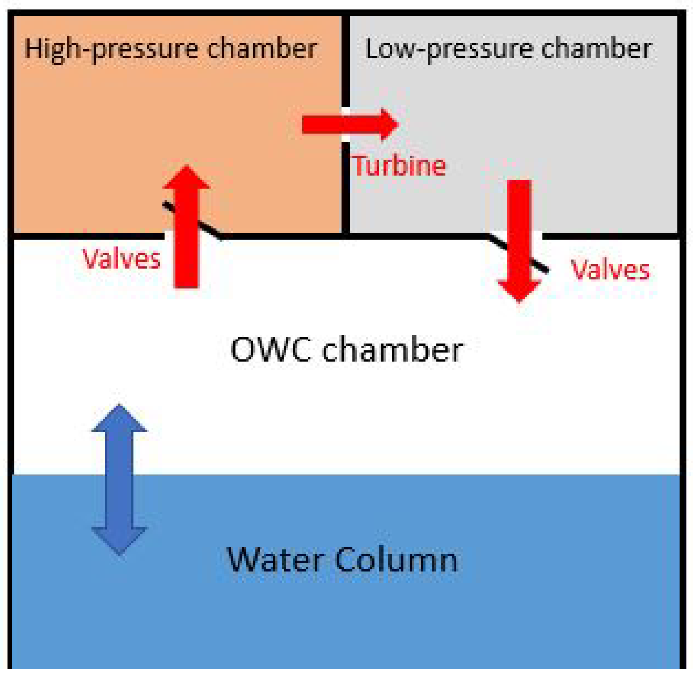
The Tupperwave device is a closed-circuit OWC using non-return valves and two accumulator chambers to create a smooth unidirectional flow across a unidirectional turbine. Figure 1 describes schematically the working principle of the device under study. The motion of the water column alternatively pushes air into the High Pressure chamber (HP chamber) through the HP valves when rising and sucks air out from the Low Pressure chamber (LP chamber) through LP valves when falling. Due to the flow restriction across the turbine, a pressure differential builds between the two chambers, and the air flows in a relatively steady manner from the HP chamber to the LP chamber across a unidirectional turbine. Therefore, the Tupperwave working principle does not only aim at using a unidirectional turbine, but also at smoothing the unidirectional air flow. The objective is to facilitate the conversion from pneumatic power to mechanical power by the unidirectional turbine and to reach a turbine efficiency close to the maximum efficiency obtained in the constant flow condition. The incentive of the Tupperwave principle is that unidirectional turbines can reach efficiencies close to 95% in such conditions. Ultimately, the Tupperwave principle aims at increasing both the electrical power output and quality, compared to a conventional OWC.
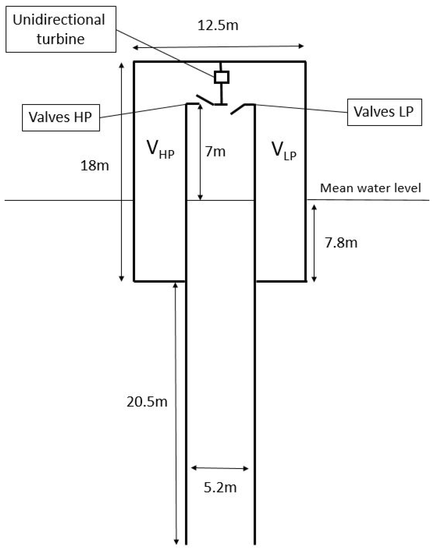
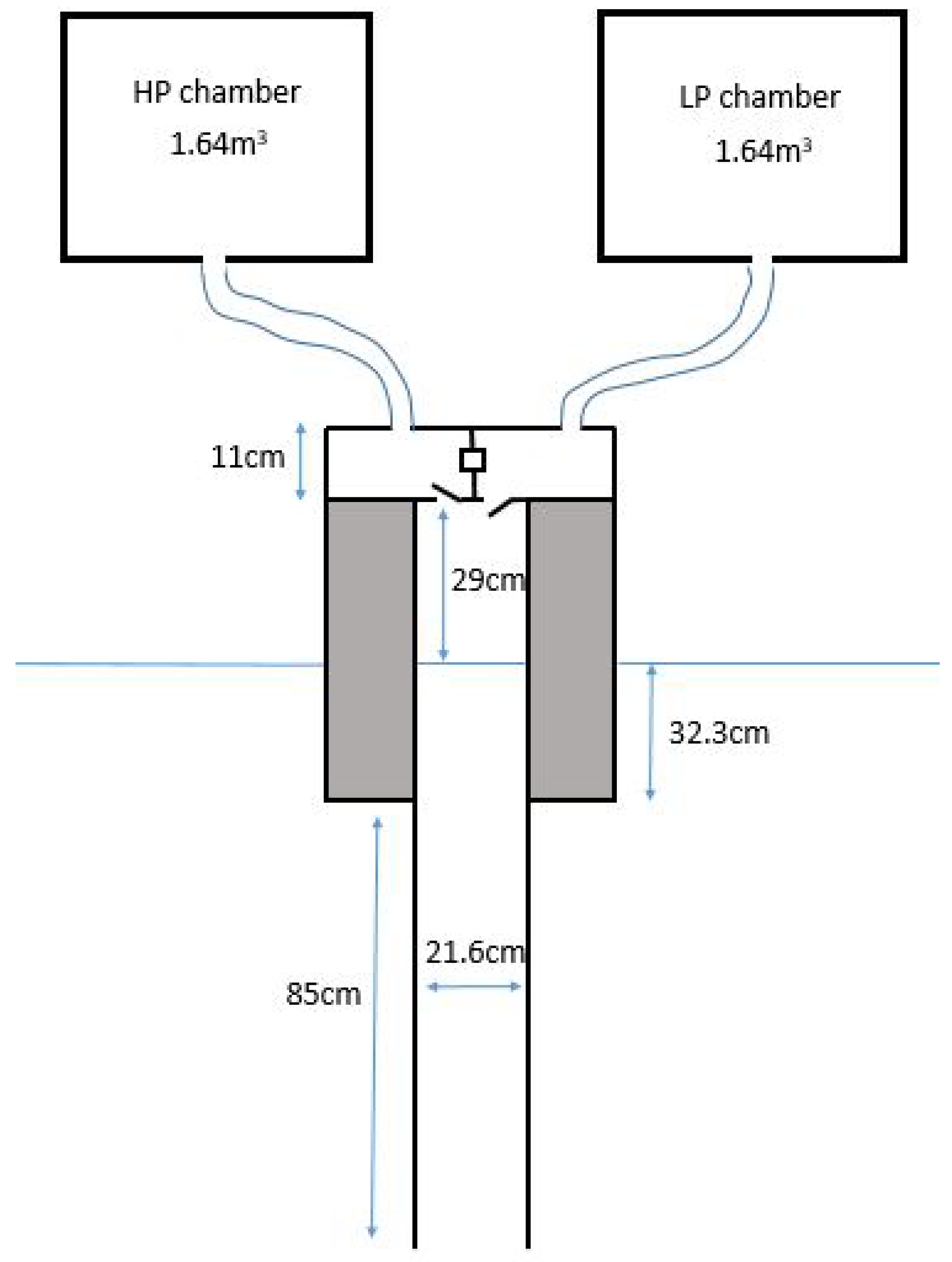
Within the scope of the Tupperwave project, a parametric study was first carried out on the chambers’ volume and turbine damping [5]. The results showed that larger chambers lead to better pneumatic power smoothing. Since it had been decided to apply the Tupperwave principle to a floating spar buoy, the entire buoyancy volume is used for the accumulator chambers. Figure 2 displays the geometry of the full-scale Tupperwave device. The volumes of the HP and LP chambers have a constant value of 950 m each.
In this paper, various methods to model the Tupperwave device are described, and the results are compared. In Section 2, a numerical model of the device is developed based on the linear waves and potential flow theories using the Ordinary Differential Equations (ODEs), linking hydrodynamic and thermodynamic physical quantities. Hereinafter, this model is identified as Numerical Model 1. Section 3 presents another model using the Computational Fluid Dynamics (CFD) software ANSYS CFX. In the scope of this document, this model will be designated as Numerical Model 2. The results of Numerical Model 2 are compared against the results of Numerical Model 1. Section 4 presents the physical modelling of the device at 1/24th scale tested in a wave tank. The physical results are compared against the results of Numerical Model 1. The paper does not present results comparing the three models simultaneously. Although Numerical Model 1 is quite flexible, easily adapting its parameters, Numerical Model 2 and the physical model are subject to several constraints, which made it difficult to have a set of numerical simulations and physical tests with comparable parameters and conditions for the three approaches. Nevertheless, the comparisons presented are still of interest and useful to show the viability of the Tupperwave concept, as well as the relevance of the different methods. In Section 5, the influence of valves and turbine damping on the device efficiency in converting the absorbed wave power into useful pneumatic power is studied using both physical observations and numerical simulations.
2. Numerical Model 1
The numerical model of the Tupperwave device presented in this section uses ODEs coupling hydrodynamic and thermodynamic variables.
2.1. Hydrodynamics
The spar buoy structure and the water column are considered as two rigid bodies moving only in heave in the waves relative to each other [6]. The model is based on linear waves and potential flow theories. Both bodies are subject to the Cummins equation, and their coupled heave motions (denoted as Index 1 for the buoy and 2 for the piston) can be written in time-domain as:
where are the bodies’ masses; are the bodies heave motion added masses at infinite frequency (proper and cross modes); are the restoring force coefficients; are the radiation impulse functions for heave motions (proper and cross modes), which are functions of the radiation damping coefficients ; are the wave excitation forces. is the reciprocating force due to the pressure in the OWC chamber acting on both bodies and is calculated as: where S is the internal water free-surface in the water column and is the excess pressure relative to the atmospheric pressure built in the OWC chamber. The viscous drag forces and are calculated as where is the equivalent drag coefficient. This force incorporates the viscous drag effects, as well as all non-linear viscous effects [7].
The frequency domain coefficients , , and are calculated using the commercial BEM solver WAMIT [8]. The four convolution integrals are called memory effect integrals. Their values depend on the history of the system, which implies their recalculation at each time step and is not practical for solving the system. By using the conventional Prony’s methods [9], it is possible to calculate each of these functions as the sum of additional unknowns {, }, which are the solutions of additional first order equations that will be solved along with the system of Equations (1)a,b. For this research, was taken, which adds 16 first order equations to the system.
2.2. Thermodynamics
In the Tupperwave device, air is exchanged between three different air chambers. Unlike for the conventional OWC where the OWC chamber is open to the atmosphere, the air in the Tupperwave device is flowing in a closed-circuit. Figure 1 displays the different thermodynamic variables in the three chambers. The volume of the OWC chamber varies with the relative motion of the device structure and water column as:
where is the volume of the OWC chamber when both bodies are at rest and S is the horizontal internal water surface area of the water column.
The compressibility of the air in the three chambers is modelled using the linearised isentropic relationship between pressure and density:
where p is the excess pressure in the chamber relative to the atmospheric pressure . It was shown in [10] that the isentropic assumption provides a very satisfactory approximation of the air spring-like effect in the chambers.
In each chamber, the mass balance equation gives:
where and are the air volumetric flows rates flowing respectively in and out of the chamber and is the density of the incoming flow.
Moreover, the mass variation in a chamber can be written as:
Equations (2)–(5) applied to the three chambers of the device lead to the three coupled thermodynamic ODEs, also coupled with the hydrodynamic ODEs (1)a and (1)b:
where , , and are the volumetric air flow rates across the turbine, the HP valve, and the LP valve. The sign convention for the volumetric flow rates is given by the arrow directions in Figure 1.
The air flow rate across a real turbine is a function of the turbine diameter, rotational speed, and pressure head. In the following sections, the turbine will be modelled by an orifice, and the relationship between flow rate and pressure drop is considered as quadratic:
where is the damping coefficient of the orifice and is a function of its diameter.
The valves are non-return valves that close when the pressure head across the valves is under a certain positive opening pressure . is defined as for the HP valve and as for the LP valve. When opened, the relation between flow rate and pressure drop is:
where and are the damping coefficients of the valve, a function of its opening area.
3. Numerical Model 2
This section presents the modelling of the Tupperwave device using Computational Fluid Dynamics (CFD), which is based on Reynolds Averaged Navier–Stokes (RANS) equations, which provides more advantages in overcoming the potential flow weaknesses in handling problems that involve strong nonlinearity, dispersion, wave breaking, complex viscosity, turbulence, and vortex shedding.
3.1. Model Setup
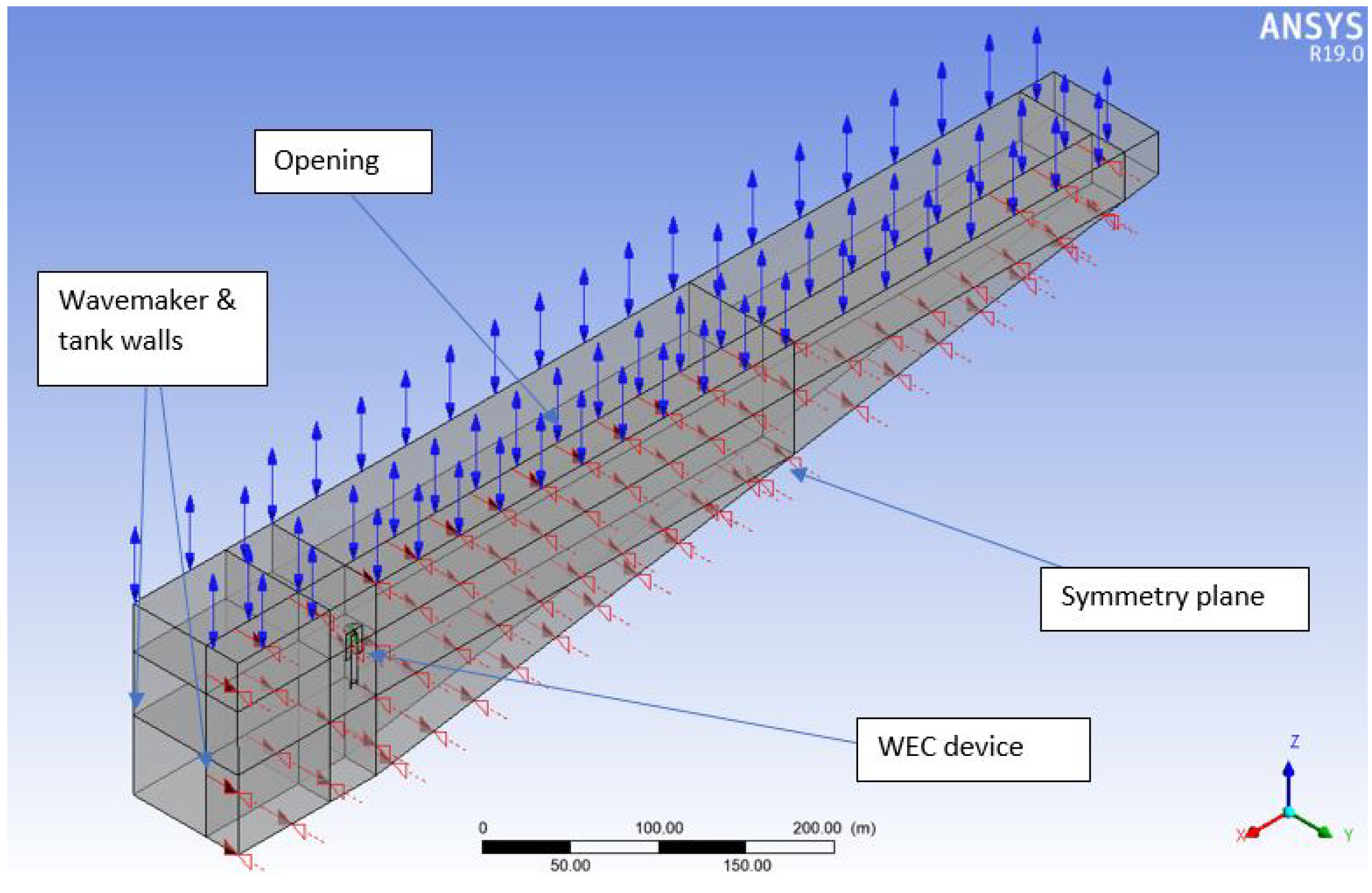
The Tupperwave device was simulated in a 3D numerical wave tank with the software package ANSYS CFX V19.1. The geometry of the device was generated with the software Solidworks and brought to the air and water domain of the numerical wave tank.
The dimensions of the domain were set according to the guidelines given in [11]. The water depth at the device location was 100 m. The following boundary conditions were applied to the flow domain:
- Non-slip conditions prescribed at the wave energy device and the boundaries representing the tank walls;
- Non-slip wall conditions applied to the wave dissipation ramp and the tank bottom;
- Opening condition applied to the top wall. The mass and momentum transported through this boundary were constrained by an opening pressure and direction model, with 0 Pa relative pressure. The volume fraction of the opening for air was set to 1.0 and that of water to 0.0. The temperature was set to 17 °C;
The 3D wave tank and boundary conditions are displayed in Figure 3.
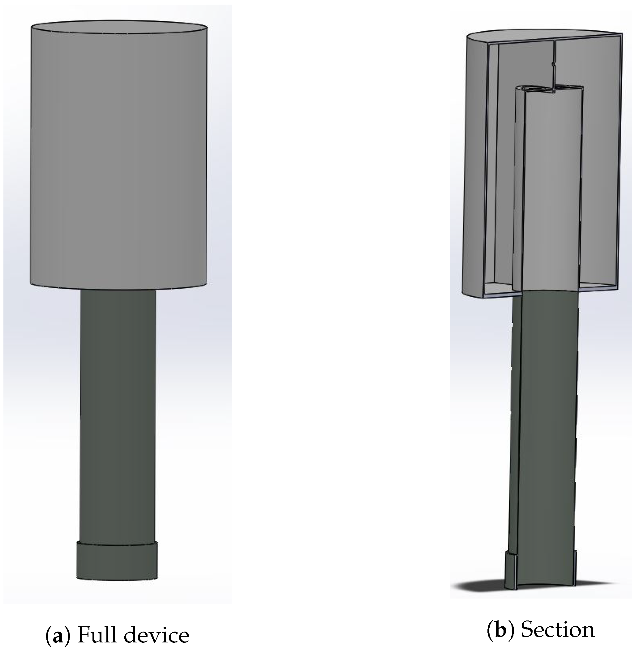
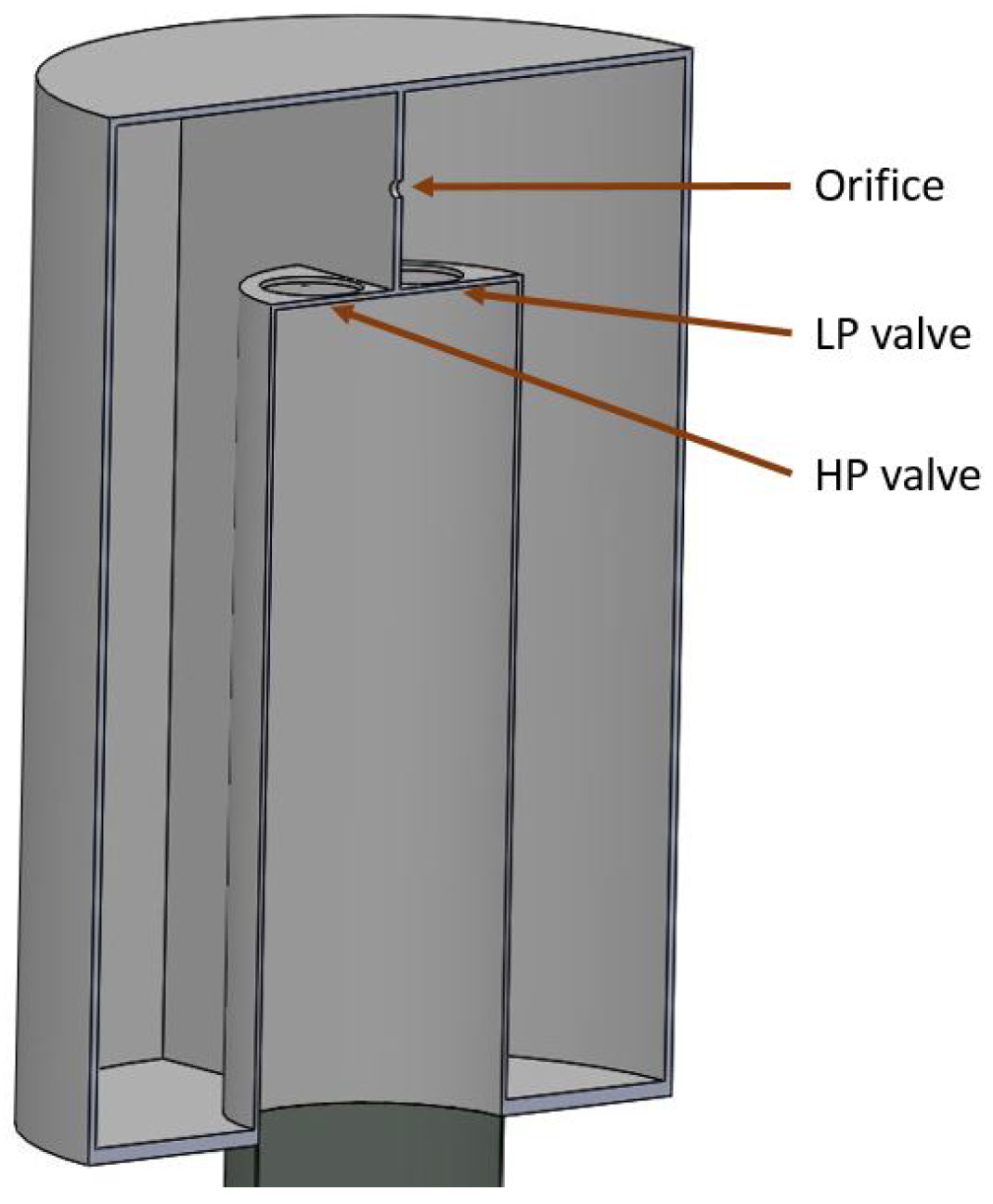
Figure 4a,b displays the three-dimensional drawings of the Tupperwave device used in the CFD model. The orifice representing the turbine is 22 cm in diameter. To maximise the opening area of the valves, there were two round HP valves of 1.8 m in diameter connecting the OWC chamber to the HP chamber and two round LP valves connecting the LP chamber to the OWC chamber. The valves were modelled as surface interfaces, with a logical expression that defined the condition of open or closed. The condition is based on the sign of the pressure difference on both sides of the valves. The open condition allowed air to flow through unimpeded, while the closed condition placed a barrier across the face of the valve. The pressures were measured as a volume average value in 5 cm-thick volumes immediately above and below the valves, over the whole area of the valves. The opening pressure of the valves was set to = 0 Pa. This is an idealistic representation of the valves. In reality, the valve design is likely to be much more complex and the opening pressure to be a non-null value, but this representation indicates the upper limit of how good valves can be. The orifice and valves are displayed in Figure 5.
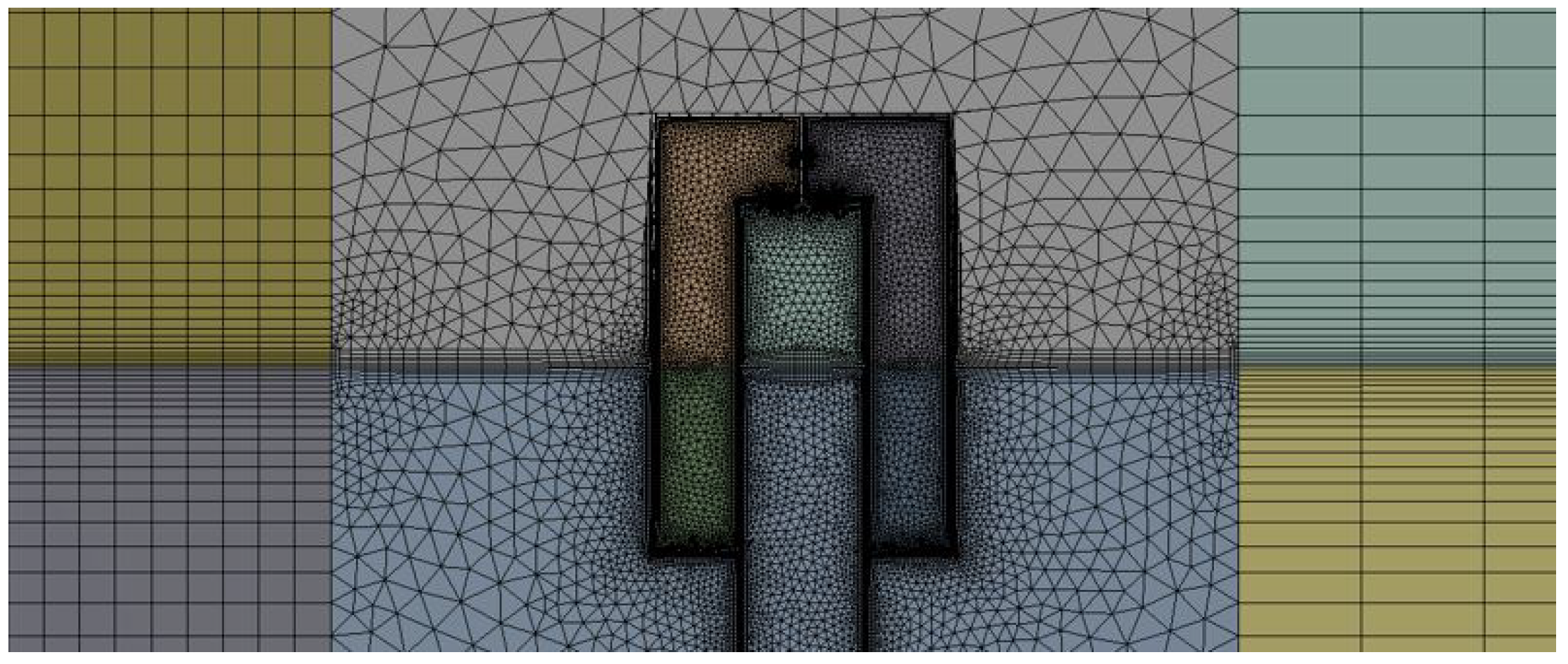
A volumetric mesh was generated for the fluid and solid domains using ANSYS Workbench meshing v19.1. The mesh is a hybrid hexa/tetra/prism mesh. This meshing strategy was chosen since it is a flexible and inexpensive type of mesh. A finer resolution mesh was employed in the areas of interest, and a boundary layer with appropriate thickness was used near the walls and in the turbine. At least four cells were present across the thickness of the device’s solid walls. Between the wave source and the OWC device, the mesh was uniform along the x-axis and non-uniform along the y-axis, with a finer mesh region around the free-surface. This mesh contained 1,497,806 nodes and 4,066,389 elements in the fluid domain and 839,440 nodes and 1,983,223 elements in the solid domain. Figure 6 displays the mesh in the vicinity of the device.
The analysis type was a transient, homogeneous, multiphase, thermal model analysis, with the standard free-surface model. The turbulence model employed to represent turbulent fluctuations was the k-wShear Stress Transport (SST) model. Interphase transfer was achieved with the free-surface model. The total simulation duration was 400 s with a time step interval of 0.06 s.
Difficulties in modelling the complete floating device were encountered when coupling the device motion with the compressible fluid model. This issue forced the authors to simplify the problem and give the device a fixed position, facilitating the computation.
Geometry preparation, meshing, and pre-processing were done on a Dell Z-book laptop with a four-core, Intel i7 processor, and 16 GB of RAM. The full model simulations were run on a 64-core, 157 GB RAM Amazon Web Services (AWS) EC2 virtual machine cluster over two compute nodes.
3.2. CFD Results
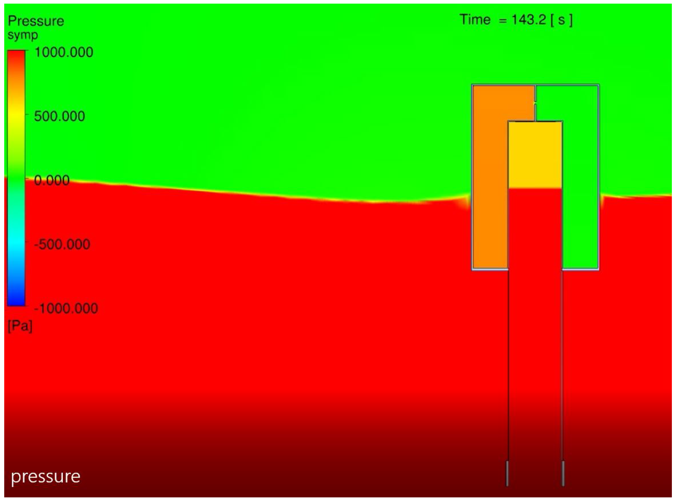
Figure 7 displays an image of a simulation run with a fixed buoy in two meter-high regular waves at 8-s periods. A video of the simulation has been added to the paper as a Supplementary File. It gives a good view of how the device works. The clear pressure difference all along the simulation was visible between the HP chamber on the left and the LP chamber on the right.
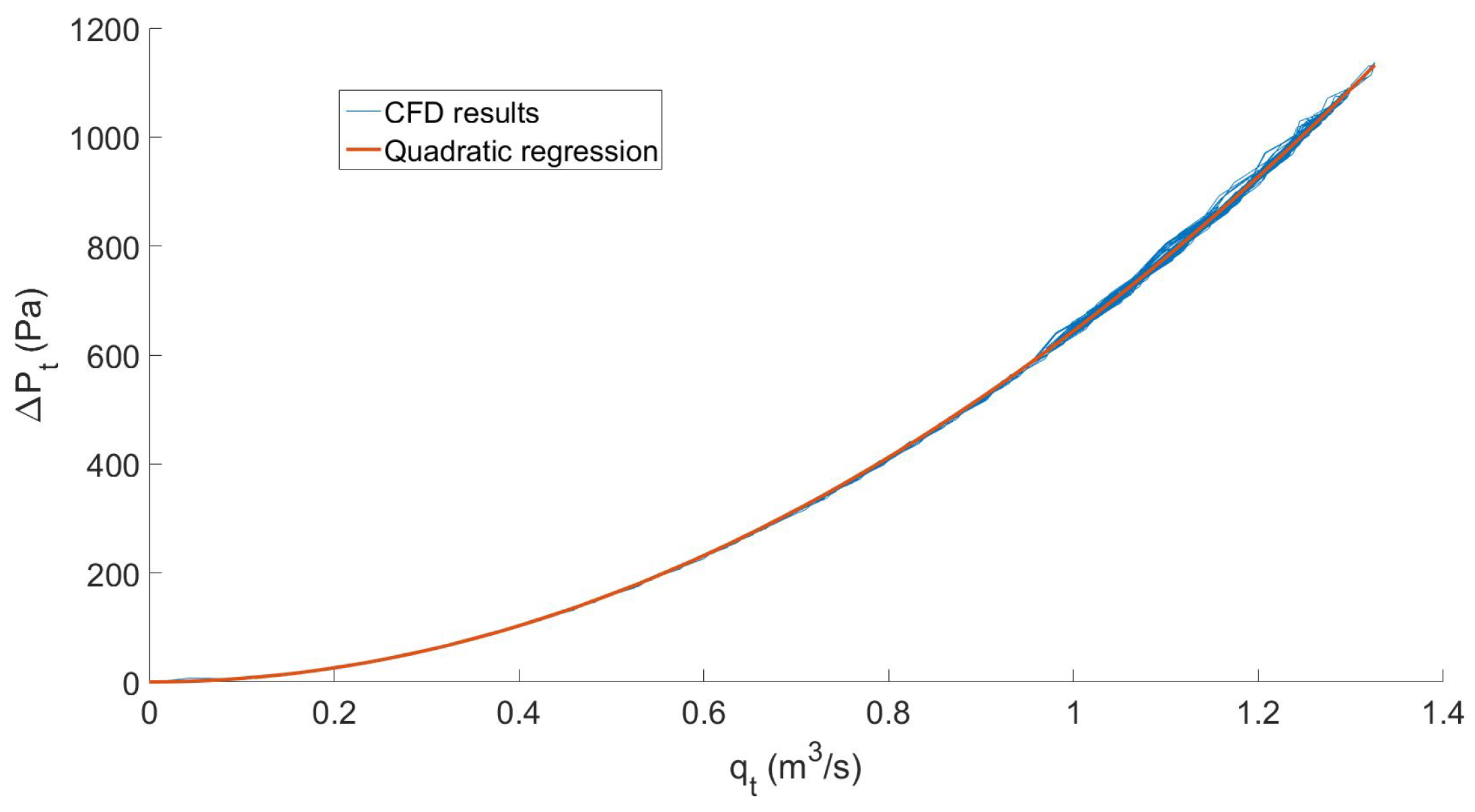
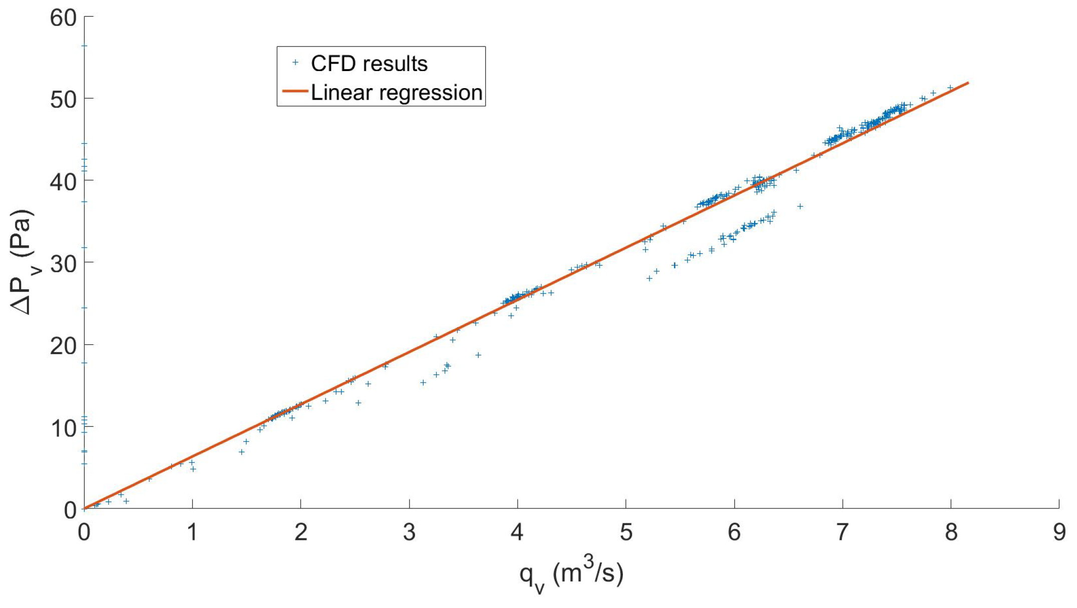
The damping coefficient of the orifice was determined by quadratic regression in Figure 8. A coefficient of determination (or value) of 0.9996 was obtained. Being close to one, the coefficient indicated good regression fitting. For the valves, it was observed that the relationship between flow rate and pressure drop was not quadratic, but linear, as can be seen on Figure 9. This is equivalent to in Equation (8). was assessed by linear regression with a coefficient of determination of 0.9828.
With the purpose of fairly comparing the numerical models, the damping coefficients of the orifice and valves obtained in the CFD simulations were used in the Numerical Model 1, and the floater was also considered to be fixed. Results from Numerical Models 1 and 2 are compared in Figure 10. The Internal Water Surface (IWS) refers to the free-water surface elevation within the OWC chamber. Good agreement was obtained between the models, both on the relative motions of the bodies (IWS) and on the pressures in the different chambers. Small high-frequency fluctuations were observed in the pressures obtained by the CFD model due to fast unnecessary obstruction of the valves. Because the volumes used to measure the pressures on both sides of the valves were very small and close together, their average pressure values thus tended to equalize briefly every couple of time steps, closing the valves for one time step and creating a small pressure peak. The pressure fluctuations were especially visible in the OWC chamber, which was the smallest chamber. This did not happen in Numerical Model 1 because the pressures were assumed uniform in each chamber.
The power absorbed from the waves by the device is the mechanical power applied by the IWS on the air inside the OWC chamber and is calculated as:
This power was converted into pneumatic power and distributed across the valves and the turbine. The pneumatic power available at the turbine or across the valves was calculated as the product of the pressure drop times the volumetric flow rate:
Only the power across the turbine is useful for electrical power production. The pneumatic power across the valves was dissipated under the form of heat due to viscous losses. The efficiency of the valves describes their capacity to let the air pass from one chamber to the next without dissipating energy. As a result of the valves’ operation, the initial pneumatic power extracted from the waves was made available to the unidirectional turbine. The average efficiency of the valves was therefore defined as:
It was shown in [13] that the Tupperwave device is competitive relatively to its corresponding conventional OWC when the valves’ efficiency is higher than 80%. With the valves implemented in this CFD model, the valves’ efficiency reached 95%. Since the valves were assumed to be ideal, 95% valve efficiency is probably the upper limit achievable.
4. Physical Modelling
4.1. Experimental Setup
A tank testing campaign of the Tupperwave device at the model scale was carried out in the Deep Ocean Basin of the Lir-National Ocean Test Facility at the MaREICentre, Ireland. The device was built at the model scale and equipped with all necessary instrumentation to monitor its behaviour fully. For the underwater part of the device, a Froude scaling factor , which was close to 1/24th scale, was applied. However, the Tupperwave working principle relies on the air compressibility in the HP and LP chambers, which is not scalable with Froude similarity law. The Froude scaling similarity law requires to scale down the 950 m chambers by , which gives . With such small volumes and in the pressure conditions of the experiment, the air in the chambers would act as incompressible. According to a method suggested in [14], the volumes of the HP and LP chambers were scaled by to properly scale down the compressibility effect of the air, which gave per chamber. This scaling law for the chambers size requires much larger size chamber than the Froude similarity would indicate. Unlike for the full scale, it was impossible to fit both chambers on the laboratory scale device as their volume largely exceeded the overall volume of the device. The alternative at a small scale was to locate the main volume of the HP and LP chambers outside of the device and to connect them to two smaller chambers on the device with flexible pipes. The reservoirs were located on the pedestrian bridge above the water. The flexible pipes were chosen as lightweight and flexible as possible to reduce their influence on the floating device motion. Part of the pipes’ weight was supported by bungee ropes. Figure 11 displays a schematic of the Tupperwave model-scale device, and Figure 12 shows a picture of the Tupperwave physical model in the water.
Ideally, the same scaling method applied to the HP and LP chambers should be used for the OWC chamber, adding a third flexible pipe connecting the OWC chamber to another reservoir outside the device. However, air compressibility in the OWC chamber is not essential for the device working principle, and the OWC chamber was therefore scaled down using Froude scaling for simplicity.
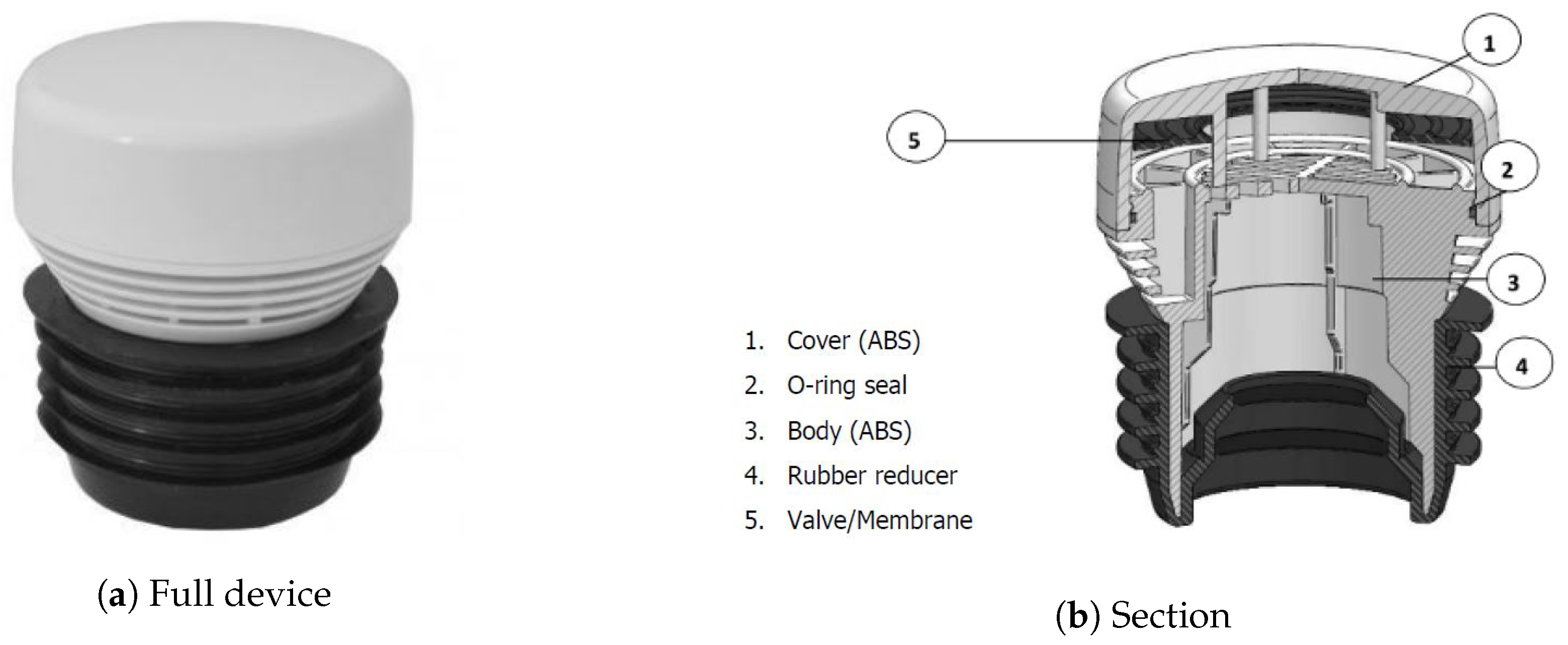
The most appropriate valves found on the market were the Capricorn MiniHab HypAirBalance; see Figure 13a,b.
They are passive normally closed air admittance valves from the plumbing market. A rubber membrane contained in the valve obstructs its opening by gravity. When sufficient pressure is applied, the rubber membrane is lifted up, and the valve opens. Their light weight allowed their use in the small-scale Tupperwave physical model.
A large number of tests were undertaken. For the regular waves, two wave heights (2 m and 4 m) were tested with periods ranging from 5–14 s. Note that these are the full-scale equivalent dimensions. Eight irregular sea states of various significant wave heights and peak periods were also tested. In each wave condition, the device was tested with three different orifices numbered from 1–3 with increasing damping (decreasing orifice diameter).
4.2. Experimental Results
It was observed experimentally that the relationship between pressure drop and flow rate across the valves was quadratic. This relationship is characteristic for turbulent flows. The Reynolds number across the valves was assessed, and was in the order of , which demonstrates that the regime was turbulent [15]. This is equivalent to in Equation (8), and the relationship between pressure drop and flow rate across the valves becomes:
The valves opening pressure was found close to 70 Pa (equivalent to 1686 Pa at full scale).
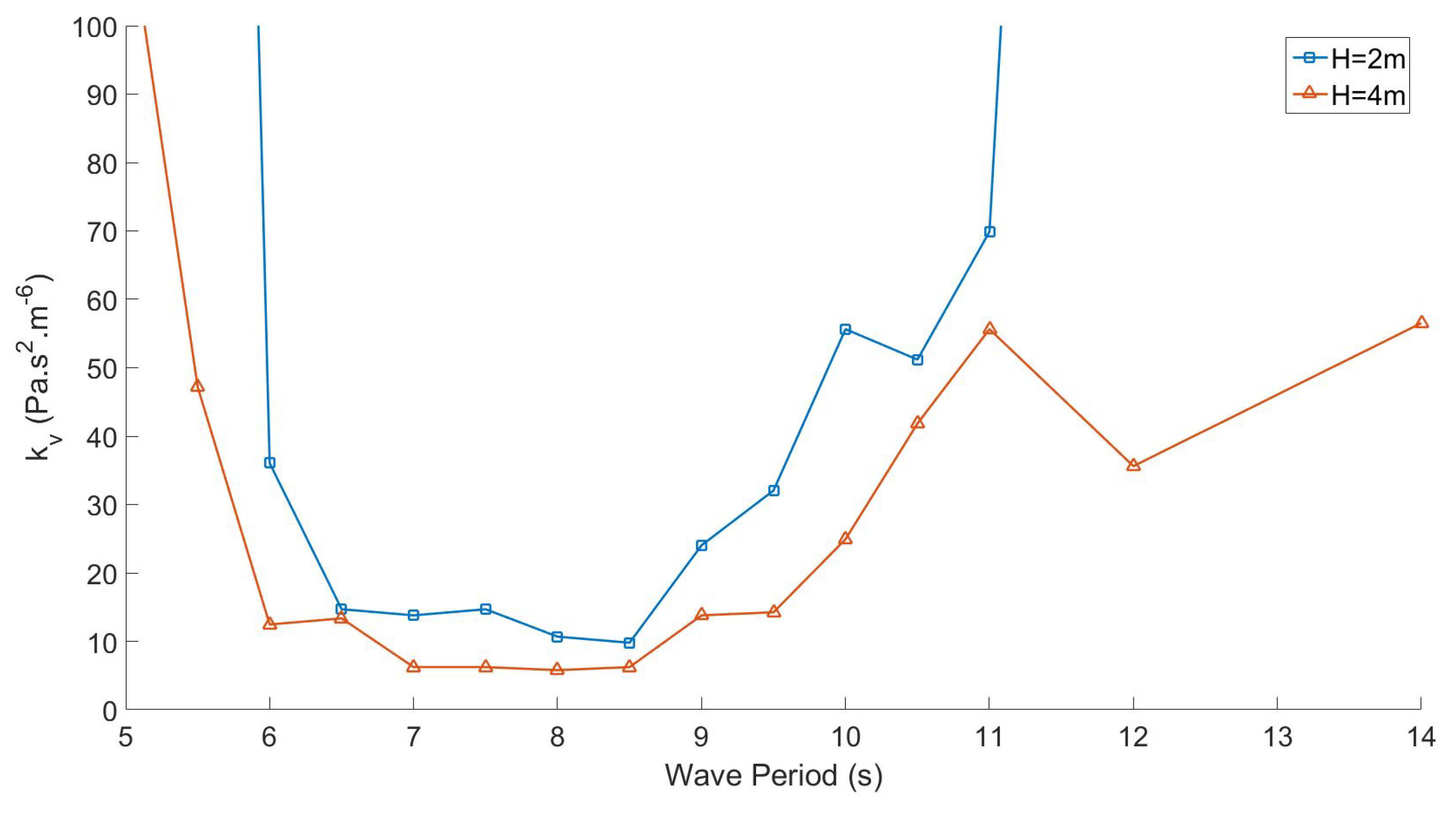
The damping coefficient of the passive valves was assessed in every test. It was found that its value changed significantly depending on the wave conditions and device excitation. This phenomenon is particularly obvious in regular waves. Figure 14 displays the damping coefficient of the HP valves in regular waves for the two wave heights tested. It was observed that when the device was close to resonance (for 6.5 s 8.5 s, near its resonance), large pressure drops across the valves were created. The valves were thus open fully, and their damping coefficient was small. On the contrary, when the device was poorly excited by the waves (for 6.5 s and 8.5 s), the valves did not open fully and created large damping (i.e., large losses). The variation of damping coefficient led to a variation in the valves’ efficiency to rectify the flow through the turbine. This is a major difference compared to the ideal valves used in the CFD model that are open instantaneously with a given opening area and therefore with a given damping and given efficiency. The dependence of the valves’ efficiency on the damping is addressed in the next section.
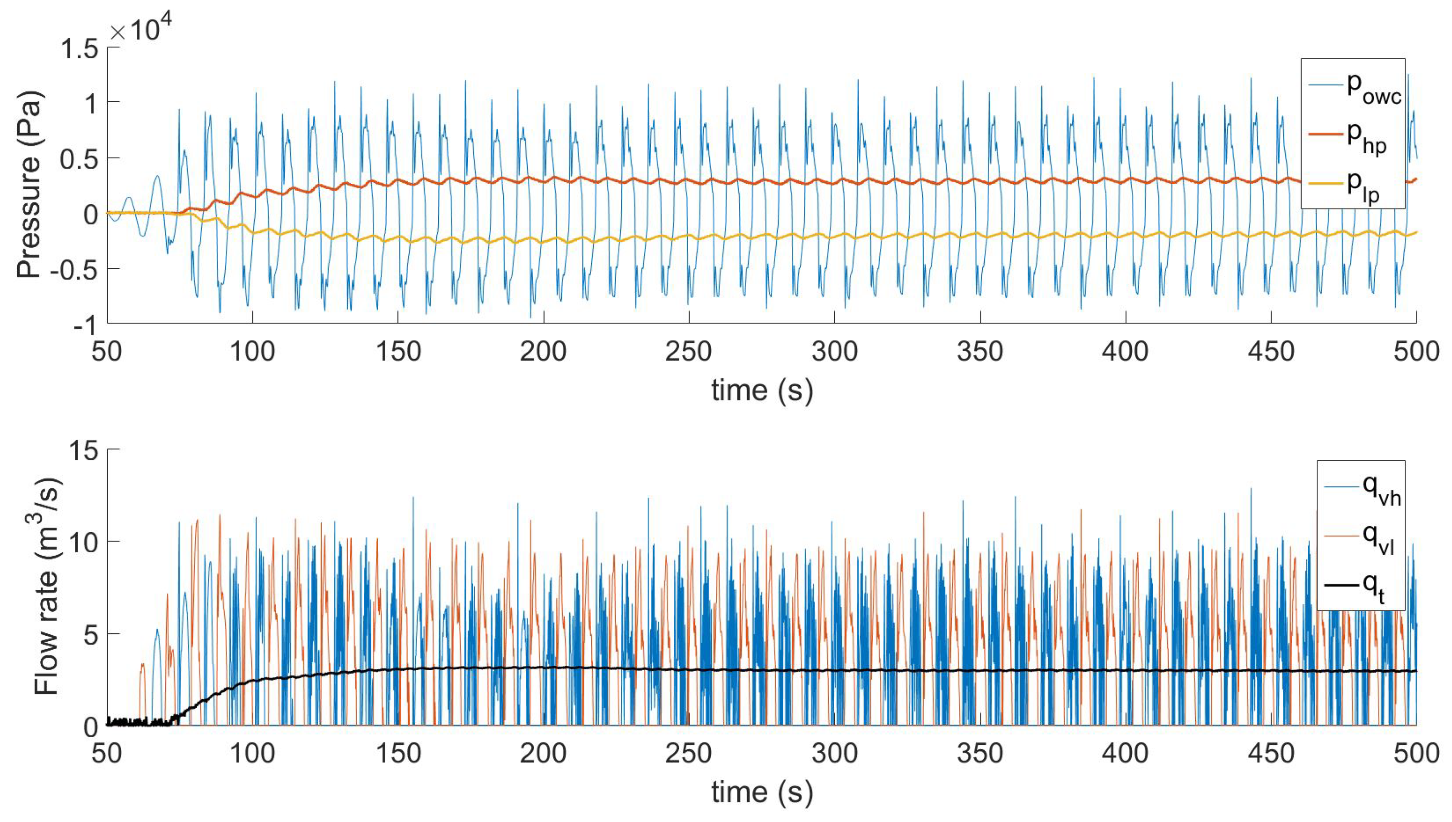
The tank testing campaign of the Tupperwave device proved that the Tupperwave principle was viable and that it actually built a steady pressure differential between the HP and LP chambers, hence creating a very smooth unidirectional flow across the turbine. To illustrate this feature, Figure 15 displays the time series of the pressures in the chambers and flows across the valves and turbine for a 2 m-high regular wave of a 9-s period (full-scale equivalent). More details on the physical tank testing of the Tupperwave model can be found in [16].
The results of the physical tank testing were used to validate the first numerical model of the device. Very good agreement was obtained between numerical and physical models. Details on the numerical model validation using the tank testing results can be found in [17]. Moreover, the tank testing provided physical observations on the real behaviour of the device and especially of the valves.
5. Device Conversion Efficiency
In this section, the ability of the device to convert the absorbed wave power into available power to the turbine is analysed in regular waves using both physical and numerical approaches.
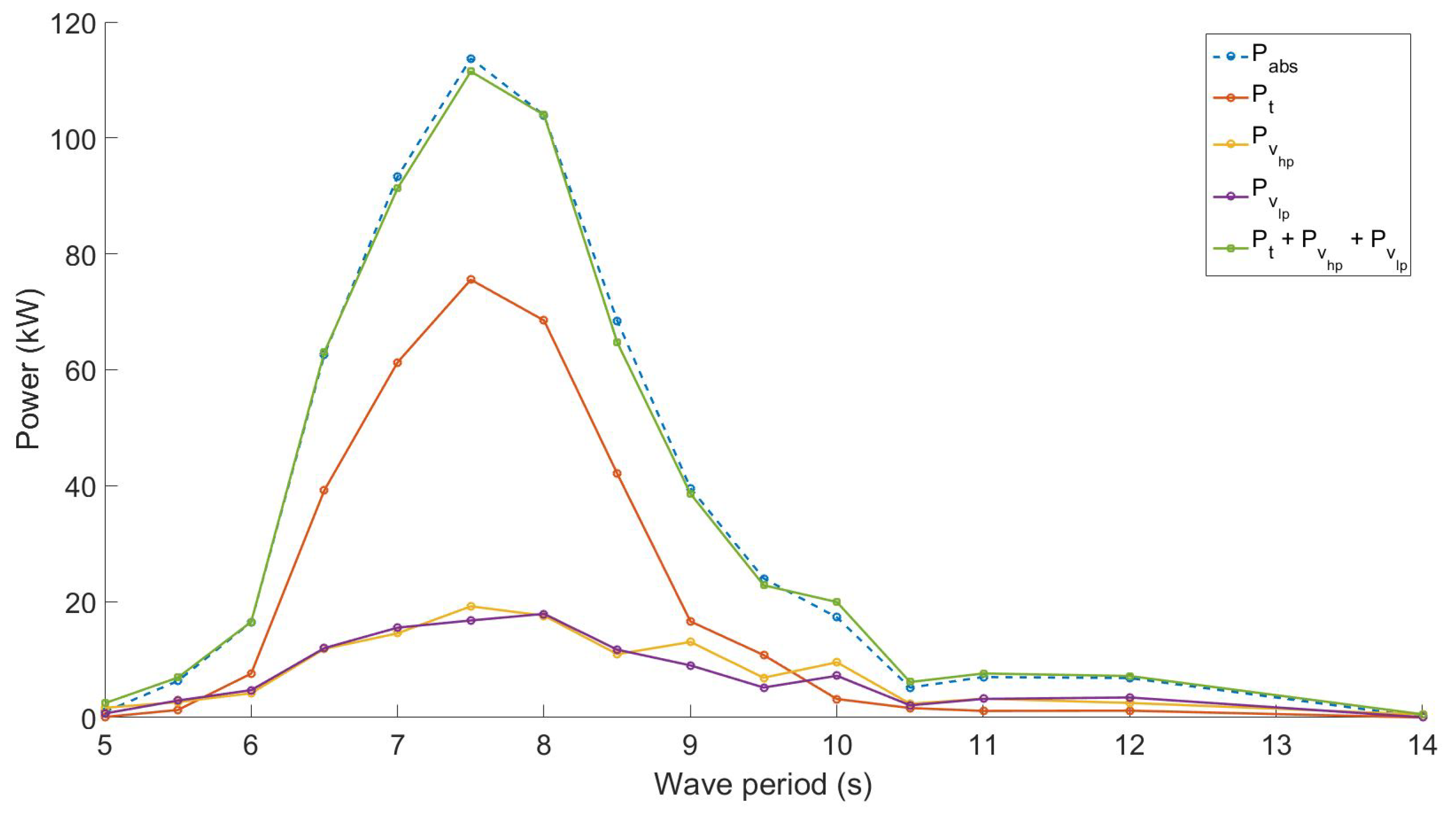
This analysis was initially driven by physical observations made during the tank testing. Figure 16 compares the average absorbed power on regular waves to the sum of the dissipated pneumatic power in the valves and orifice, for the case of Orifice 2, and shows that the absorbed power was entirely dissipated in the valves and the turbine.
The average valves’ efficiency can therefore be rewritten as:
At model scale, the variation of air density in the device chamber was small compared to the atmospheric density, and therefore, it was assumed that in all chambers. The average pneumatic power across the turbine can be calculated using the damping coefficient and the average mass flow across the turbine:
Since the mass flow across the turbine was almost constant, it is a reasonable approximation to write:
The total power dissipated in the turbine can be approximated by:
Using Equation (12), the instantaneous power dissipated in the LP and HP valves can be expressed as:
As the HP and LP valves were identical, their damping was the same, . Furthermore, since the HP and LP valves were never open at the same time, we have:
Hence, Equation (17) becomes:
Moreover, since the circuit was closed, the valves were crossed by the same amount of air as the turbine in the overall simulation. The air was constantly flowing across the turbine, while the air was only flowing alternatively across each valve less than half of the time. The average value of the sum of the mass flow rate across the valves can be roughly approximated as a constant flow of value . Figure 15 illustrates this fact, and it can be written as:
The average pneumatic power dissipated across the valves was obtained by averaging Equation (19) and using Equations (15) and (20):
Finally, the average pressure head across the turbine can be written as:
Eventually, the average valve efficiency can be approximated from the turbine and valve damping characteristics using the equation:
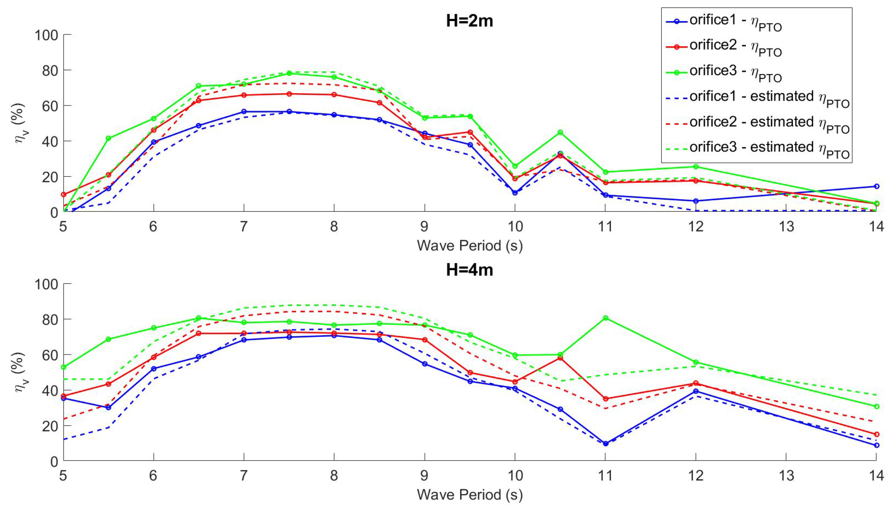
The valves’ efficiency was not only dependent on the valves’ damping coefficient (i.e., opening area), but it was a function of the ratios and . Results obtained from Equation (24) were tested against the actual efficiency of the valve obtained in tank testing. Figure 17 compares the measured efficiency to the estimation for H = 2 m and H = 4 m and for the three tested orifices. Equation (24) yields a good approximation of the measured valves’ efficiency. Despite the approximations used in its derivation, the formula shows that, in order to maximise the Tupperwave valves efficiency, the opening pressure of the valves needs to be small compared to the average pressure drop across the valves, and the damping coefficient of the valves needs to be small compared to the damping coefficient of the turbine.
Figure 17 also shows that the maximum valve efficiency reached during the tank testing was between 50% and 80%, depending on the orifice. The maximum efficiencies were reached for wave periods 6.5 s 8.5 s, where the valves’ damping coefficient was the smallest (see Figure 14). In accordance with Formula (24), the best efficiencies were reached with Orifice 3, which had the largest damping . This was due to the fact that became smaller, thus increasing .
Moreover, orifices with larger damping created greater average pressure difference between the HP and LP chamber , decreasing the ratio and, consequently, increasing . Physically, one can explain this phenomenon with the following reasoning: higher represents more difficulty for the passage of air through the turbine, thus increasing the pressure drop between the HP and LP chambers and reducing the flow across the turbine; since the circuit of air was closed, the flow across the valves was also reduced, which implies a lower velocity of the air through the valves; in turn, lower velocity represents less friction losses, and ultimately led to higher efficiency of the valves for a smaller orifice.
Therefore, for a given valve damping coefficient, the efficiency of the valves to not dissipate the absorbed power from the waves became higher for larger values of the turbine damping coefficient, . However, similarly to a conventional OWC device, the absorbed wave power was also largely dependent on .
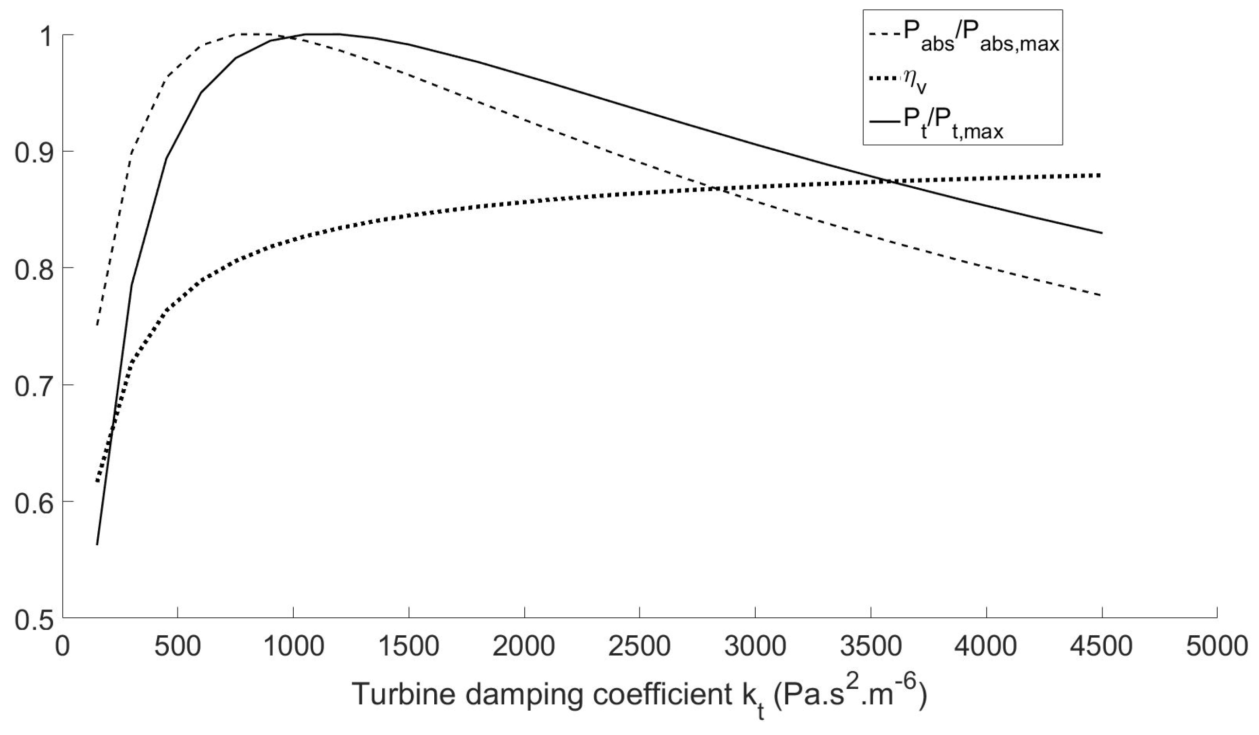
Figure 18 displays the results of a parametric study carried out with Numerical Model 1 on the full-scale device to find the optimal coefficient maximising the power production of the device in 2 m-high regular waves of eight-second periods. The damping coefficient of the valves was set to = 5 Pa s m and the opening pressure = 150 Pa. On the one hand, and similarly to conventional OWC devices, the power absorbed by the device (dashed line) was largely dependent on and reached a maximum for a certain value of . On the other hand, and as discussed in the previous paragraph, the valves’ efficiency to convert the absorbed power into useful pneumatic power (dotted line) became higher for larger values of . In the end, finding the optimal damping coefficient maximising the power made available to the turbine (solid line) was a trade-off between maximising the wave power absorption by the device and maximising the valves’ efficiency.
6. Conclusions
In this paper, the modelling of the Tupperwave device was approached with three different methods, which all enabled various observations of the device behaviour.
The first approach, using potential flow theory and hydrodynamic and thermodynamic ordinary differential equations, was revealed to be the most efficient and quickest method to model the Tupperwave device in various conditions and was the most appropriate to carry out parametric optimisation. The second approach, using three-dimensional CFD with the software Ansys CFX, was the longest to implement, and the results within the duration of the Tupperwave project were limited due to the slow computational time. The third approach, using physical tank testing at 1/24th scale, provided real-life observations of the device and especially of the valves.
Ideal active valves were tested in the CFD model with zero opening pressure and a large opening area. With those valves, 95% of the absorbed wave power was converted into pneumatic power available to the turbine. Real passive off-the-shelf valves from the plumbing market were tested in the physical model. Being passive, the valves only opened well when the device was close to resonance, leading to a varying efficiency depending on the wave conditions, but also on the tested orifice-turbine. Their maximum efficiency ranged from 50–80%. The CFD model and in particular the physical models both provided a validation of the first model.
From observations made numerically and physically, it was shown that the valves’ efficiency was a function of the ratio between the valve and turbine dampings . While larger turbine damping increased the valve efficiency, lower values of allowed larger wave power absorption by the device. Finding the optimal value is therefore a trade-off between maximising wave power absorption and maximising the valve efficiency.
Supplementary Materials
The following are available online at https://www.mdpi.com/2077-1312/7/2/23/s1.
Author Contributions
Conceptualization, P.B., M.V., A.D., and J.M.; investigation, P.B., M.V., and A.D.; writing, original draft, P.B.; writing, review and editing, P.B., M.V., A.D., and J.M.; funding acquisition, M.V., A.D., and J.M.
Funding
The authors would like to acknowledge funding received through OCEANERA-NETEuropean Network (OCN/00028).
Conflicts of Interest
The authors declare no conflict of interest. The funders had no role in the design of the study; in the collection, analyses, or interpretation of data; in the writing of the manuscript, or in the decision to publish the results.
Abbreviations
The following abbreviations are used in this manuscript:
| OWC | Oscillating Water Column |
| HP | High Pressure |
| LP | Low Pressure |
| CFD | Computational Fluid Dynamics |
References
- Falcão, A.F.; Henriques, J.C. Oscillating-water-column wave energy converters and air turbines: A review. Renew. Energy 2016, 85, 1391–1424. [Google Scholar] [CrossRef]
- Lopes, B.S.; Gato, L.M.; Falcão, A.F.; Henriques, J.C. Test results of a novel twin-rotor radial inflow self-rectifying air turbine for OWC wave energy converters. Energy 2018. [Google Scholar] [CrossRef]
- Lopes, B. Construction and Testing of a Double Rotor Self-Rectifying Air Turbine Model for Wave Energy Recovery Systems. Language of Reference: Portuguese. Master’s Thesis, Tecnico Lisboa, Lisboa, Portugal, 2017. [Google Scholar]
- Falcão, A.F.; Henriques, J.C.; Gato, L.M. Self-rectifying air turbines for wave energy conversion: A comparative analysis. Renew. Sustain. Energy Rev. 2018, 91, 1231–1241. [Google Scholar] [CrossRef]
- Vicente, M.; Benreguig, P.; Crowley, S.; Murphy, J. Tupperwave-preliminary numerical modelling of a floating OWC equipped with a unidirectional turbine. In Proceedings of the 12th European Wave and Tidal Energy Conference (EWTEC), Cork, Ireland, 27 August–1 September 2017. [Google Scholar]
- Sheng, W.; Alcorn, R.; Lewis, A. Assessment of primary energy conversions of oscillating water columns. I. Hydrodynamic analysis. J. Renew. Sustain. Energy 2014, 6, 053113. [Google Scholar] [CrossRef] [Green Version]
- Giorgi, G.; Ringwood, J.V. Consistency of viscous drag identification tests for wave energy applications. In Proceedings of the 12th European Wave and Tidal Energy Conference (EWTEC), Cork, Ireland, 27 August–1 September 2017. [Google Scholar]
- Lee, C.H.; Newman, J.N. WAMIT User Manual. WAMIT, Inc.: Chestnut Hill, MA, USA, 2006. [Google Scholar]
- Sheng, W.; Alcorn, R.; Lewis, A. A new method for radiation forces for floating platforms in waves. Ocean Eng. 2015, 105, 43–53. [Google Scholar] [CrossRef]
- Benreguig, P.; Vicente, M.; Murphy, J. Anisentropic study of the Tupperwave device. Energy 2018. submitted. [Google Scholar]
- Finnegan, W.; Goggins, J. Numerical simulation of linear water waves and wave–structure interaction. Ocean Eng. 2012, 43, 23–31. [Google Scholar] [CrossRef] [Green Version]
- Silva, M.; Vitola, M.D.A.; Pinto, W.; Levi, C. Numerical simulation of monochromatic wave generated in laboratory: Validation of a cfd code. In Proceedings of the 23 Congresso Nacional De Transporte Aquaviário, Construção Naval e Offshore, Rio de Janeiro, Brazil, 25–29 October 2010; pp. 25–29. [Google Scholar]
- Benreguig, P.; Kelly, J.F.; Murphy, J. Wave-to-Wire model development and validation for two OWC type wave energy converters, part II: From pneumatic to electrical energy. Energy 2018. submitted. [Google Scholar]
- Falcão, A.F.; Henriques, J.C. Model-prototype similarity of oscillating-water-column wave energy converters. Int. J. Mar. Energy 2014, 6, 18–34. [Google Scholar] [CrossRef]
- Tennekes, H.; Lumley, J.L.; Lumley, J. A First Course in Turbulence; MIT Press: Cambridge, MA, USA, 1972. [Google Scholar]
- Benreguig, P.; Murphy, J.; Sheng, W. Model scale testing of the Tupperwave device with comparison to a conventional OWC. In Proceedings of the ASME 2018 37th International Conference on Ocean, Offshore and Arctic Engineering OMAE2018, Madrid, Spain, 17–22 June 2018. [Google Scholar]
- Benreguig, P.; Murphy, J. Wave-to-Wire model development and validation for two OWC type wave energy converters, part I: From wave to pneumatic energy. Energy 2018. submitted. [Google Scholar]
Figure 1.
Schematic diagram of the Tupperwave device concept.

Figure 2.
2D schematic of the full-scale Tupperwave device.

Figure 3.
3D wave tank and boundary conditions.

Figure 4.
3D design of the full-scale Tupperwave device implemented in the CFD model.

Figure 5.
Section view of the symmetry plane of the Tupperwave device.

Figure 6.
Mesh in the vicinity of the device.

Figure 7.
2D picture of the full-scale Tupperwave device in two-meter high regular waves of 8-s periods.
Figure 7.
2D picture of the full-scale Tupperwave device in two-meter high regular waves of 8-s periods.

Figure 8.
Flow rate across the turbine-orifice as a function of the pressure drop with quadratic regression ( = 0.9996).
Figure 8.
Flow rate across the turbine-orifice as a function of the pressure drop with quadratic regression ( = 0.9996).

Figure 9.
Flow rate across the HP valves as a function of the pressure drop with linear regression ( = 0.9828).
Figure 9.
Flow rate across the HP valves as a function of the pressure drop with linear regression ( = 0.9828).

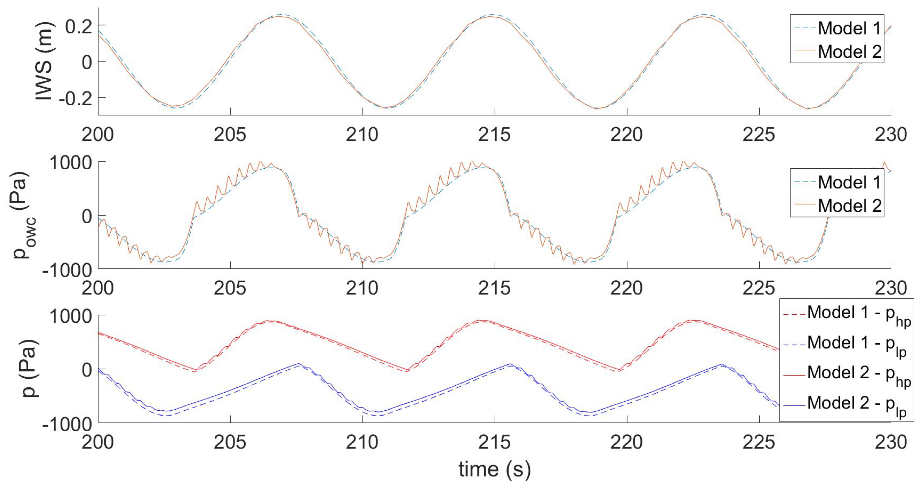
Figure 10.
Internal Water Surface (IWS) elevation and excess pressures obtained in OWC, HP and LP chambers obtained by Numerical Models 1 and 2 for 2 m-high and 8 s-period regular waves.
Figure 10.
Internal Water Surface (IWS) elevation and excess pressures obtained in OWC, HP and LP chambers obtained by Numerical Models 1 and 2 for 2 m-high and 8 s-period regular waves.

Figure 11.
Schematic of the model-scale conventional OWC and Tupperwave devices.

Figure 12.
Physical model of the Tupperwave device.

Figure 13.
MiniHab HypAirBalance from Capricorn used in the Tupperwave small-scale model.

Figure 14.
HP valve damping coefficient in regular waves (full-scale equivalent).

Figure 15.
Time series of pressures in the chambers and flows across the valves and turbine for a 2 m-high regular wave of a nine-second period (full-scale equivalent) obtained in tank testing.
Figure 15.
Time series of pressures in the chambers and flows across the valves and turbine for a 2 m-high regular wave of a nine-second period (full-scale equivalent) obtained in tank testing.

Figure 16.
Average absorbed power from the waves and dissipated powers across valves and orifice (full-scale equivalent).
Figure 16.
Average absorbed power from the waves and dissipated powers across valves and orifice (full-scale equivalent).

Figure 17.
Valve efficiency obtained in regular waves compared to the efficiency estimated via Formula (24).
Figure 17.
Valve efficiency obtained in regular waves compared to the efficiency estimated via Formula (24).

Figure 18.
Parametric study of the turbine damping coefficient to maximise pneumatic power made available to the turbine.
Figure 18.
Parametric study of the turbine damping coefficient to maximise pneumatic power made available to the turbine.

© 2019 by the authors. Licensee MDPI, Basel, Switzerland. This article is an open access article distributed under the terms and conditions of the Creative Commons Attribution (CC BY) license (http://creativecommons.org/licenses/by/4.0/).
Share and Cite
MDPI and ACS Style
Benreguig, P.; Vicente, M.; Dunne, A.; Murphy, J. Modelling Approaches of a Closed-Circuit OWC Wave Energy Converter. J. Mar. Sci. Eng. 2019, 7, 23. https://doi.org/10.3390/jmse7020023
AMA Style
Benreguig P, Vicente M, Dunne A, Murphy J. Modelling Approaches of a Closed-Circuit OWC Wave Energy Converter. Journal of Marine Science and Engineering. 2019; 7(2):23. https://doi.org/10.3390/jmse7020023
Chicago/Turabian StyleBenreguig, Pierre, Miguel Vicente, Adrian Dunne, and Jimmy Murphy. 2019. "Modelling Approaches of a Closed-Circuit OWC Wave Energy Converter" Journal of Marine Science and Engineering 7, no. 2: 23. https://doi.org/10.3390/jmse7020023
Note that from the first issue of 2016, this journal uses article numbers instead of page numbers. See further details here.