Wave (Current)-Induced Pore Pressure in Offshore Deposits: A Coupled Finite Element Model


1
State Key Laboratory of Ocean Engineering, Department of Civil Engineering, Shanghai Jiao Tong University, Shanghai 200240, China
2
Griffith School of Engineering, Griffith University Gold Coast Campus, Queensland, QLD 4222, Australia
3
School of Engineering, University of Aberdeen, Aberdeen AB24 3UE, UK
4
School of Engineering, University of Bradford, Bradford BD7 1DP, UK
*
Author to whom correspondence should be addressed.
J. Mar. Sci. Eng. 2018, 6(3), 83; https://doi.org/10.3390/jmse6030083
Submission received: 10 May 2018
/
Revised: 7 June 2018
/
Accepted: 3 July 2018
/
Published: 6 July 2018
(This article belongs to the Special Issue Coastal Geohazard and Offshore Geotechnics)
Abstract
:The interaction between wave and offshore deposits is of great importance for the foundation design of marine installations. However, most previous investigations have been limited to connecting separated wave and seabed sub-models with an individual interface program that transfers loads from the wave model to the seabed model. This research presents a two-dimensional coupled approach to study both wave and seabed processes simultaneously in the same FEM (finite element method) program (COMSOL Multiphysics). In the present model, the progressive wave is generated using a momentum source maker combined with a steady current, while the seabed response is applied with the poro-elastoplastic theory. The information between the flow domain and soil deposits is strongly shared, leading to a comprehensive investigation of wave-seabed interaction. Several cases have been simulated to test the wave generation capability and to validate the soil model. The numerical results present fairly good predictions of wave generation and pore pressure within the seabed, indicating that the present coupled model is a sufficient numerical tool for estimation of wave-induced pore pressure.
1. Introduction
The phenomenon of wave and seabed interaction has drawn great interest among coastal geotechnical engineers over the past decade. The reason for this growing attention is that offshore infrastructure, such as platforms, pipelines and breakwaters, have encountered structural failure due to wave-induced seabed instability [1,2,3] rather than construction or material failure.
Considerable investigations into the wave-seabed interaction have been carried out in past decades. The methods for investigating the wave-seabed interaction problem mainly include three types, namely the uncoupled method, the semi-coupled method, and the fully coupled method [4,5,6]. The uncoupled method in investigating a wave-induced seabed response mainly occurred in earlier studies. There is no data exchange between the fluid motion and the seabed deformation. The porous and deformable seabed was regarded as a rigid and impermeable medium in a fluid domain, and the dynamic wave pressure on the seabed surface was replaced by a simplified wave pressure equation in the seabed domain [7,8]. The semi-coupled method, also called the one-way coupled method, has been widely used in investigating the wave-seabed interaction problem in past decades. The wave motion was firstly calculated through CFD (computational fluid dynamic) solver, which is usually coded by FDM (finite difference method) and FVM (finite volume method). Then, the dynamic response of the seabed was analyzed by FEM (finite element method), in which the dynamic wave pressure extracted from the fluid domain was applied on the seabed surface through linear interpolation [9,10]. The semi-coupled method could consider the effects of the dynamic wave loading on the seabed. However, the feedback of the deformed seabed to the wave motion is not taken into account [11,12,13,14]. The fully coupled method could simulate both the wave motion and the dynamic seabed response simultaneously, in which a real-time data exchange is required between the two domains. It is easy to see that the fully coupled method should be the most accurate method for studying the wave-seabed interaction problem. However, in investigating the wave-seabed interaction problem, the fully coupled method is scarcely used in the previous research.
To implement the wave propagating process, it is necessary to build a wave-maker in the wave field, where the progressive wave is generated and propagates over a porous seabed combined with currents. Based on the FEM, we use an internal wave-maker method for generating essentially directional waves in a two-dimensional domain using a momentum source function of the Reynolds Averaged Navier Stokes (RANS) equation proposed by Choi and Yoon [15]. The internal wave-maker was used to avoid the influence of waves reflected from the wave-maker toward the domain because the waves generated by the source function do not interact with waves reflected from inside the domain and the sponge-layer method, as proposed by Israeli and Orszag [16], has been used to absorb outgoing waves generated by the wave-maker in the present study.
To sum up, both the wave and seabed field are modelled by FEM in this study. No interface program is needed to transfer the loads between them. The structure of the present paper is illustrated as follows. Section 2 introduces the basic equations that describe the wave-seabed interaction. The revised RANS equations govern the ocean wave, while the poro-elastoplastic equations describe the mechanical behavior of the seabed under wave loading. In Section 3, the present model is validated against the analytical solution and the available data of experiments shown in the literature. This section includes the wave module verification, seabed module verification and wave-seabed interaction verification. Finally, the application of the present model on wave-induced pore pressure and liquefaction is illustrated in Section 4.
2. Theory and Methods
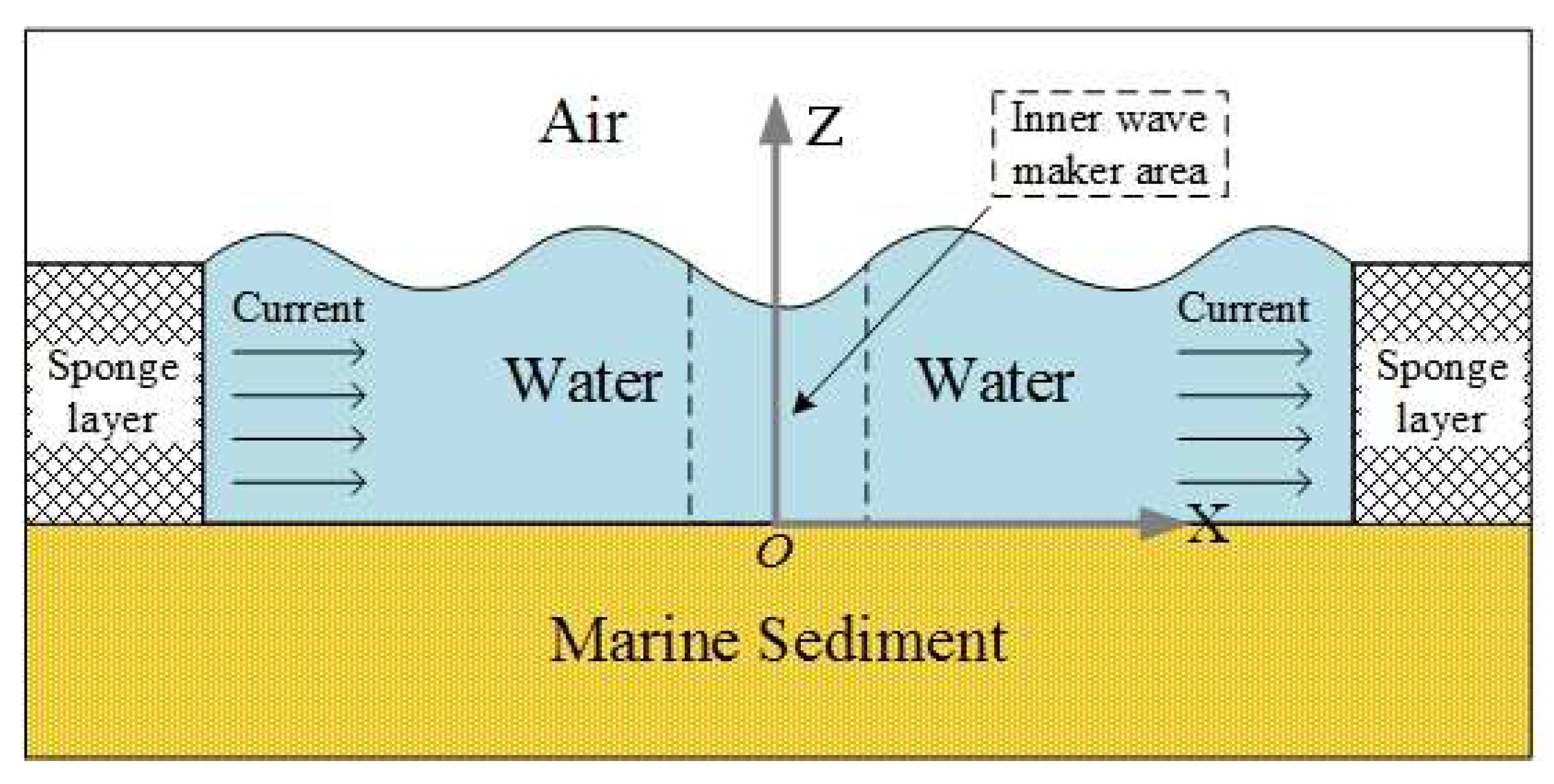
Two sub-modules are included in the present coupled approach: A wave module and a seabed module, as shown in Figure 1. The wave module is established in order to generate the wave train (current) and to describe the viscous wave propagation. The seabed module is adopted to calculate the seabed response to wave loading. Unlike any previous one-way coupled models, both sub-modules are strongly integrated in COMSOL Multiphysics (COMSOL 5.2) [17].
2.1. Wave Module
In the present study, the internal wave-maker [15] was adopted to generate a progressive wave with sponge layers [16] to absorb the wave at both ends of the numerical flume. Thus, the wave reflection from both flume ends could be efficiently eliminated.
The wave propagation above the porous seabed is described by solving the revised Reynolds Averaged Navier Stokes (RANS) equations, which are derived by integrating the momentum source term into the RANS equations, and which govern the wave motion in an incompressible fluid:
where i, j =1, 2, 3 denotes the dimensions of wave motion; is the ith component of fluid velocity; ρ is the fluid density; is the fluid pressure; is the gravitational force; and is the viscous stress tensor.
The k-ε model is employed to enclose the turbulence:
where k is the turbulent kinetic energy; ν is the kinematic viscosity; and is the eddy viscosity with . The empirical coefficients are and . The rate of stress tensor is , and , where is the Kronecker delta.
Generally speaking, there are several options to numerically generate a target wave via an internal wave-maker: Adding a mass source term to the mass conservation equation (Equation (1)) or introducing a momentum one to the equation of momentum conservation (Equation (2)). One can also use both the mass and momentum source to generate a train of wave. Theoretically, this mass/momentum source could be a point, line, or a finite volume source [18]. In this study, we will only focus on the issue of generating waves taking the method of a momentum source function in a two-dimensional domain.
To generate a wave with a momentum source, Equations (1) and (2) should be revised as follows:
where is the momentum source function within a finite area Ω. Once the simulation starts, the free surface above the source region (Ω) will vibrate instantly and the surface vibration starts to propagate to both ends of the wave flume.
To properly explain the expression of in Equation (4), it is necessary to relate the mass source function to the momentum source function for wave generation:
There are several expressions of due to different wave generation theories with a mass source. The following expression is adopted from the revised Boussinesq’s equation [19]:
where:
in which the angular frequency, , water depth, d, wave number, , wave obliquity, , and wave amplitude, , are the wave parameters adopted to obtain a target wave train. In addition, , where , in which is the wavelength and is a parameter characterizing the width of the internal wave generation region. Another expression is from the revised RANS equations proposed by Lin and Liu [18] as follows:
where is the wave velocity and is the free surface elevation above the source region. By using adequate wave parameters in Equations (5), (6) and (8), any target wave can be obtained.
Regarding the process of current generation, the steady current flow is generated in the whole domain before wave generation. Once the current becomes stable, the internal wave maker starts to generate a wave. Then, the current and wave are coupled and the wave propagates from the wave-maker zone towards the sponge areas at both ends of water domain.
2.2. Seabed Module
The wave-induced pore pressure, , varies with time at a given location as suggested by Sassa and Sekiguchi [20], and consists of two components:
where is oscillatory pore pressure and represents the residual component.
2.2.1. Oscillatory Response of Soil
On the basis of the conservation of mass equation, Biot’s consolidation equation [21] are adopted as the governing equation for oscillatory response. For two-dimensional analysis, the mass conservation is expressed as follows:
where and denote the unit weight of water and the soil porosity, respectively. The volume strain, , and the compressibility of pore fluid, , are defined as, respectively:
where are the soil displacements; is the true modulus of elasticity of pore water (taken as [22]); is the absolute water pressure; and is the degree of saturation.
The total stress, , can be decomposed into the effective stress, , and the pore pressure:
where is the Kronecker delta.
Ignoring the body forces, the equilibrium equations can be written as:
in the and directions, respectively.
Equations (10), (13), and (14) are the governing equations accounting for the oscillatory mechanism, in which the undetermined soil displacements and oscillatory pore pressure are to be solved.
In accordance with elastic theory, other stresses can be written, based on soil displacements, as:
2.2.2. Residual Response of Soil
Following Sassa and Sekiguchi [20], Liao et al. [23] extended the one-dimensional model to a two-dimensional model. In the model, the evolution of the residual pore pressure, , can be expressed as:
where represents the bulk modulus of soil. The expression of plastic volumetric strain can be written as:
where and are the parameters of material. The cyclic stress ratio, , can be expressed as:
where is the maximum amplitude of shear stress and stands for the initial effective stress in the vertical direction.
In Equation (18), the first term on the right-hand side (RHS) represents the rate of pore pressure build-up and dissipation. The second term on the RHS correlates to the effect of cyclic loading (wave repetition) on the accumulation of residual pore pressure. For more details of the poro-elastoplastic model, the readers can refer to Sassa and Sekiguchi [20] and Liao et al. [23].
2.3. Coupling Method
In this section, the coupled process of the present model will be presented, including the time scheme, the mesh scheme, and the boundary conditions.
2.3.1. Time Scheme
In the present study, the identical time scheme is applied to the whole computation domain. Since the seabed module easily reaches convergence, the time interval is set to be adaptive, thus fulfilling the requirement of fluid flow. In the traditional model, the non-matching time scheme may also work for the present case. However, it produces cumulative errors in interpolating time steps between the wave module and the seabed module. Furthermore, the non-matching time scheme makes the information exchange between the two sub-modules more complicated. In the authors’ opinion, the non-matching time scheme may reduce the accuracy of computation, thus the matching time scheme is applied to achieve a more accurate computation. FEM is used to solve all the governing equations, in combination with the second-order Lagrange elements, to ensure the second order of accuracy in evaluating the dependent variables in the computational domain. The Generalized- Method was used for the time integration when computing the dynamic soil response under water action. As a second order accurate numerical scheme, the Generalized- Method is a one-step, three-stage implicit method, in which accelerations, velocities and displacements are uncoupled. To obtain computational stability, the time interval is automatically adjusted to satisfy the Courant–Friedrichs–Lewy condition and the diffusive limit condition.
2.3.2. Mesh Scheme
In the process of solving the revised RANS equations and elastoplastic equations, two typical mesh types (i.e., the matching mesh and the non-matching mesh) are adopted in the present study. The matching mesh requires the same numbers of mesh nodes along the seabed surface. However, the solid element size is generally much larger than that of the fluid cells to reach the acceptable computation efficiency. Therefore, it is necessary to use the non-matching mesh system outside the seabed surface to make sure each part of the models is calculated in proper meshes. This treatment of the mesh scheme will not affect the process of information exchange between the two modules because the matching mesh is applied at the seabed surface; particularly, the application of non-matching mesh helps reduce the cost of CPU time and memory occupation.
The meshes used in the fluid domain are structured four-node quadrilateral elements, and the simulated results are broadly affected by the grid resolution. As such, certain criteria should be satisfied to generate a high-quality mesh to ensure a valid, and hence accurate, solution. The model grid sensitivity studies show that the model is convergent using the resolution of mainly L/60 in the x- and y- directions and H/10 in the z- direction, with a refinement factor of 2, where L is the wave length; H is the wave height; and the refinement factor represents the ratio between the grid solution of the area without structural influence and the refinement area in the vicinity of the structure. The optimal non-orthogonal FEM meshes are used in the seabed domain, which are automatically generated by the COMSOL software with a maximum element size scaling factor (MESSF) controlling the maximum allowed element size. The mesh is refined until no significant changes in the numerical solution was achieved.
2.3.3. Boundary Conditions
Appropriate boundary conditions are required to close the problem of wave-seabed interaction. Firstly, in the water domain the upper boundary of the air layer is set as a pressure outlet, where the pressure can flow in and out without any constraint. Secondly, the continuity of pressure and fluid displacement is applied at the air/water interface. Then, at the bottom boundary of the water domain, the displacement of the water particles is equal to that of the seabed surface.
Following the previous studies [24], it is acceptable to set the vertical effective stress and shear stresses to zero at the seabed surface:
where and are the wave pressure and shear stress at the seabed surface, respectively, and can be obtained from the wave model outlined in Section 2. Secondly, for the soil resting on an impermeable rigid bottom, zero displacements and no vertical flow occurs at the horizontal bottom:
2.3.4. Coupled Process
In the coupled process, the wave module is in charge of the simulation of the wave (current) propagation and determines the wave loading. The standard k-e turbulence model with the level set method (LSM) and the moving mesh method are used to model the flow of two different, immiscible fluids, where the exact position of the interface is of interest. The interface position is tracked by the LSM, with boundary conditions that account for surface tension and wetting, as well as mass transport across the interface. The LSM tracks the air-water interface using an auxiliary function. Since the displacement of the seabed surface from the seabed module will affect the flow field in the wave module, the authors use the moving mesh method to track the time-dependent displacement of the seabed surface as well.
The seabed is modeled with the PDE (partial differential equation) interface in COMSOL Multiphysics to solve all the equations describing the elastoplastic soil. The wave pressure and forces acting on the seabed are simulated by the wave module, and the results are sent to the seabed module to capture the seabed response, mainly the displacements, pore pressure, and the effective stresses. Meanwhile, the feedback of seabed response to the flow field is taken into account without any time lag, thus achieving the coupling effect. The seawater and seabed displacements at the water-seabed interface are set to be identical as well as the pressures of seawater and pore water in the seabed. This boundary condition is the basic and key requirement that ensures the coupling process stated in this research.
3. Model Validation
In this section, the coupled model is validated against the analytical solution and the available data of experiments in the literature. This section includes the wave module verification, seabed module verification, and wave-seabed interaction verification.
3.1. Wave Verification: Comparison with an Analytical Solution
To validate the wave module, the free surface elevation and the dynamic water pressure that acts on the seafloor from the coupled model is verified against an analytical solution in terms of free surface elevation and the wave pressure on the seabed. The analytical solution is calculated by the Airy wave theory and compared with our numerical solution. The input data are as follows: Wave period, T = 12.0 s; water depth, d = 30 m; wave length, L = 170 m; and wave amplitude = 2.5 m.
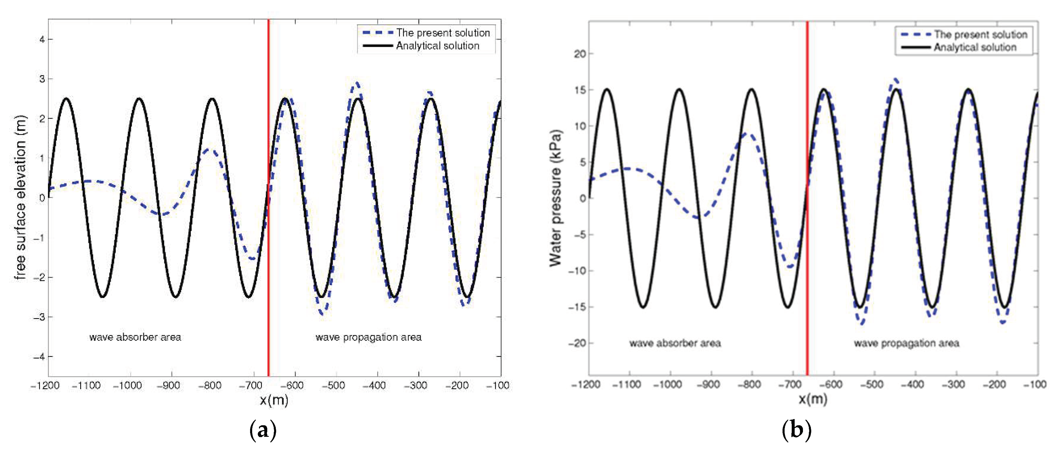
To simplify the discussion, we only show the data from the left half of the area for the analysis because the area is symmetrical. As shown in Figure 2, the domain is separated into two parts: The wave-propagation area and the wave-absorbing area. The wave is generated from the inner wave-maker zone and propagates through the entire water domain, and then absorbed by the sponge layer settled in the absorbing region. Figure 2a shows the spatial distribution of the free surface elevation from the present model and the analytical solution. The results agree well with each other except that the wave generated is slightly higher in our model than in the analytical solution. This is because when the wave approaches the absorbing area, the minor reflection from the sponge layer may amplify the wave height. This phenomenon can be alleviated by a proper absorbing coefficient or by using the data from areas away from the sponge layer. Similar results can be found in Figure 2b. The dynamic water pressure that acts on the surface of the seabed is slightly higher in our model than in the analytical solution due to the wave reflection of the sponge layer. Overall, the proposed model agrees well with the analytical solution in both the free surface elevation and the water pressure on the seabed surface.
3.2. Seabed Verification: Comparison with Experimental Data
Both oscillatory and residual soil response are verified in this section. The oscillatory pore pressure is compared with a one-dimensional compressive test conducted by Liu et al. [25], while the residual pore pressure is compared with a centrifugal test under water waves.
3.2.1. Validation of the Oscillatory Pore Pressure
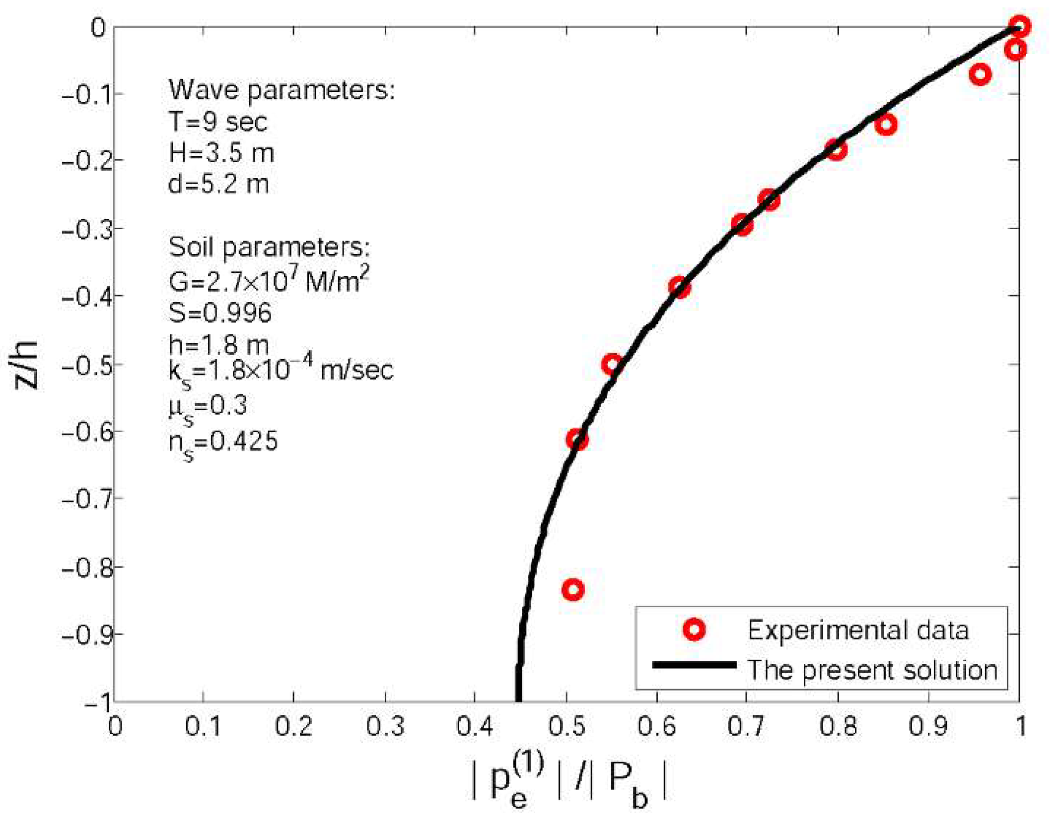
Liu et al. [25] conducted a series of one-dimensional laboratory tests to explore the vertical distribution of pore pressure under wave loading. The cylinder consisted of 10 cylindrical organic glass cells, as shown in Figure 3. Ten pore pressure gauges were installed in the sandy deposit, while one more pressure gauge was installed at the surface of the seabed. As presented in their study, only the oscillatory mechanism of the pore pressure was observed. Thus, the authors compare the results of oscillatory pore pressure with the data from laboratory experiments [25]. The simulated results of the vertical distribution of the maximum oscillatory pore pressure () are illustrated in Figure 4.
It should be noted that in the laboratory experiment, only the one-dimensional cylinder model facility was used. Thus, the wave length should be revised as infinite in the present model. Other input data used are included in Figure 4. The present model reaches a good agreement with the data from the one-dimensional experiment in the upper zone of the sandy soil. However, some discrepancy is observed in the deeper zone. There are two possible reasons that account for this discrepancy. The first is that the thickness of the sediments varies with the wave loading, which induces changes in the relative depth of sandy soil, resulting in pore pressure differences at the maximum amplitudes. Since the formulation used in the numerical approximation is based on elastic theory, accurate evaluation of the dynamic process with large soil deformation is not possible. Another potential reason is the variation of the soil density with depth in the experiment, since the sandy deposit is thick. Therefore, the response of the soil from the experimental tests may differ from that of the numerical curve, which was derived by assuming that soil properties are constant along the soil depth. However, the good agreement between the coupled model and experimental results is promising for prediction of the oscillatory pore pressure by the coupled approach.
3.2.2. Validation of the Residual Pore Pressure
Sekiguchi et al. [26] conducted the first centrifugal standing wave tests to study the instability of horizontal sand deposits by a centrifugal method. A cross section through the wave tank is shown in Figure 5. The wave tank consisted of a wave channel, a wave paddle, and a sediment trench. Standing waves were formed under the condition of a frequency, f = 8.8 Hz, under steady 50 g acceleration, along with a fluid depth of 47 mm. Waves corresponded to a prototype condition of d = 2.35 m and f = 0.176 Hz. The amplitude of the input pressure,, was 1.7 kPa. The plastic parameter, , was taken as 1.4 (corresponding to the parameter in Sekiguchi et al. [26]). The parameters were set as follows: = 55, R = , and . More detailed information can be found in Sekiguchi et al. [26]. The excess pore pressure response measured in the centrifugal test is now compared with the prediction from the present poro-elastoplastic solution. As illustrated in Figure 6, the maximum pore pressure of the centrifugal test is slightly larger than that predicted by our model. This may be due to the fact that the water waves used in the present model would attenuate over the porous seabed, leading to deviation of the water pressure from the genuine value. Except for this, the simulation reaches a good agreement with the centrifugal test.
3.3. Wave-Seabed Interaction Verification
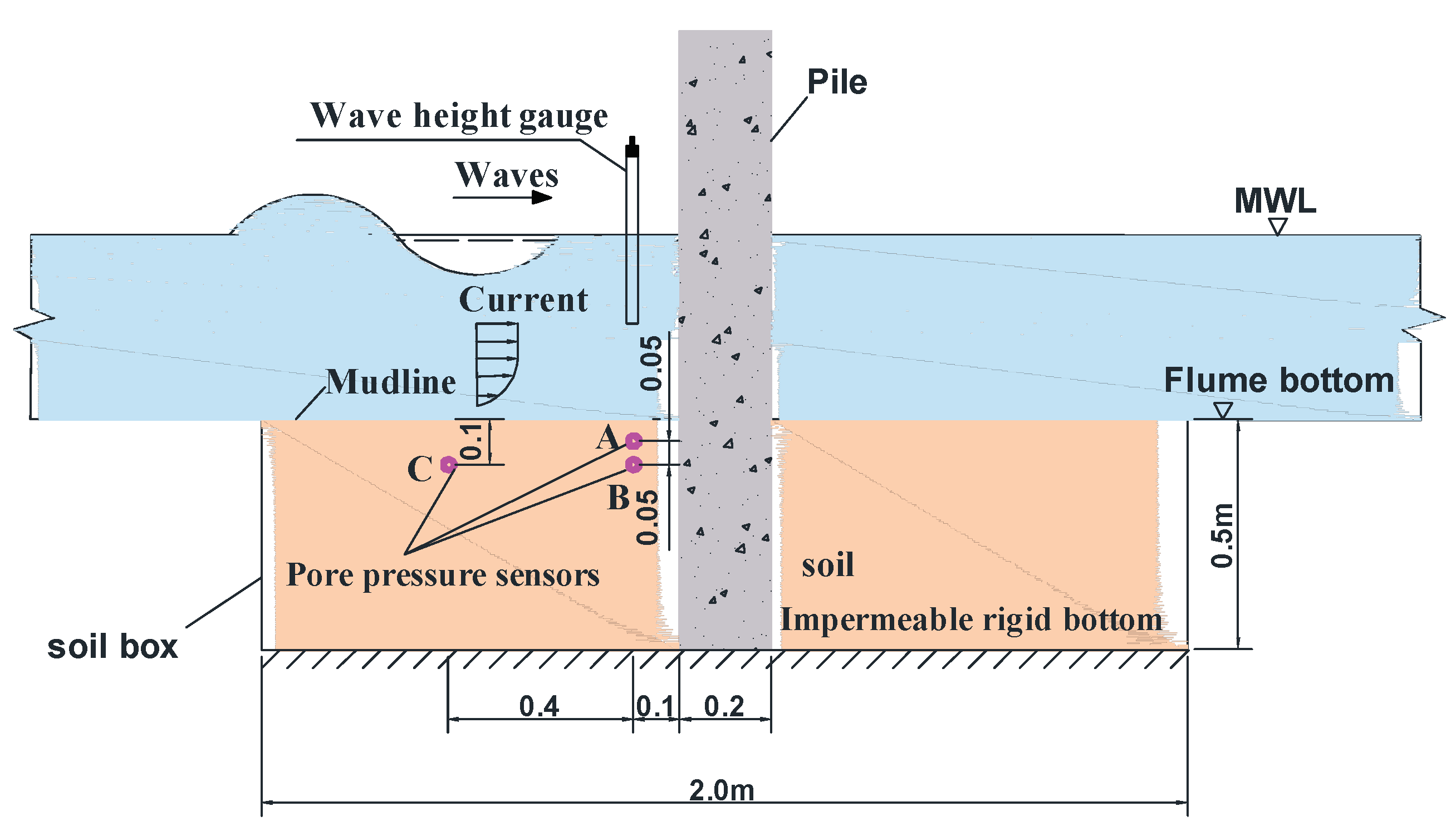
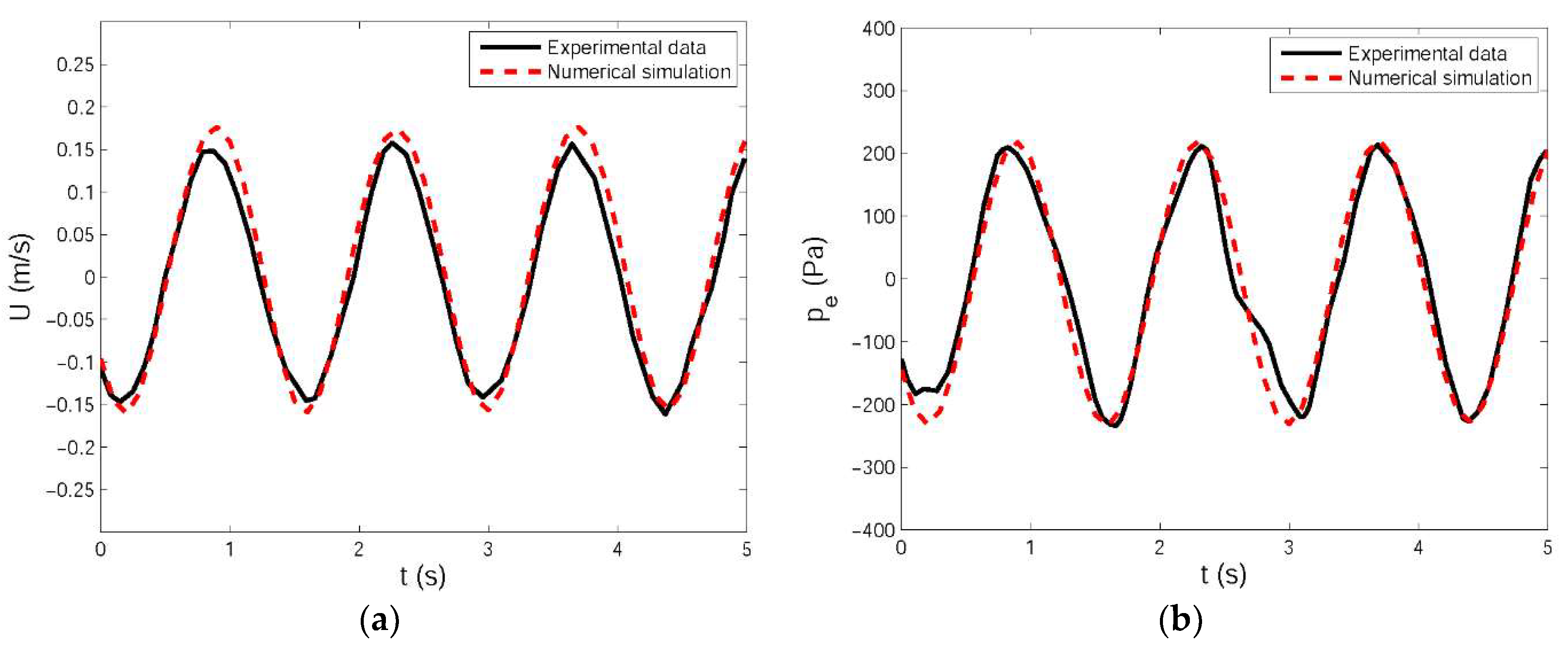
To the best of our knowledge, no laboratory experiments have been carried out to explore the interaction between the wave (or current) with the seabed except for Qi and Gao [27]. In their experiment, a series of laboratory tests was performed within a flume for the scour development and pore pressure response around a mono-pile foundation under the effect of combined wave and current. Wave, current, seabed, and structure were integrated in one model to investigate the interaction process, which provided a comprehensive understanding of the coupled model. In their experiments, the flow velocities in the wave field and pore pressure response around the pile in a finite seabed were measured simultaneously (Figure 7). Herein, the measured flow velocity and pore pressure of points far away from the mono-pile foundation, which represent the case of the wave (current)-seabed interaction without a structure, are selected for comparison with the present solution. The wave and current parameters in their experiment were: Water depth, d = 0.5 m; wave period, T = 1.4 s; wave height, H = 0.12 m; and current velocity, U0 = −0.1, 0, and +0.1 m/s. The properties of the soil provided in their paper were: Shear modulus, ; Poisson’s ratio,; permeability, ; the void ratio, ; and the soil was almost fully saturated.
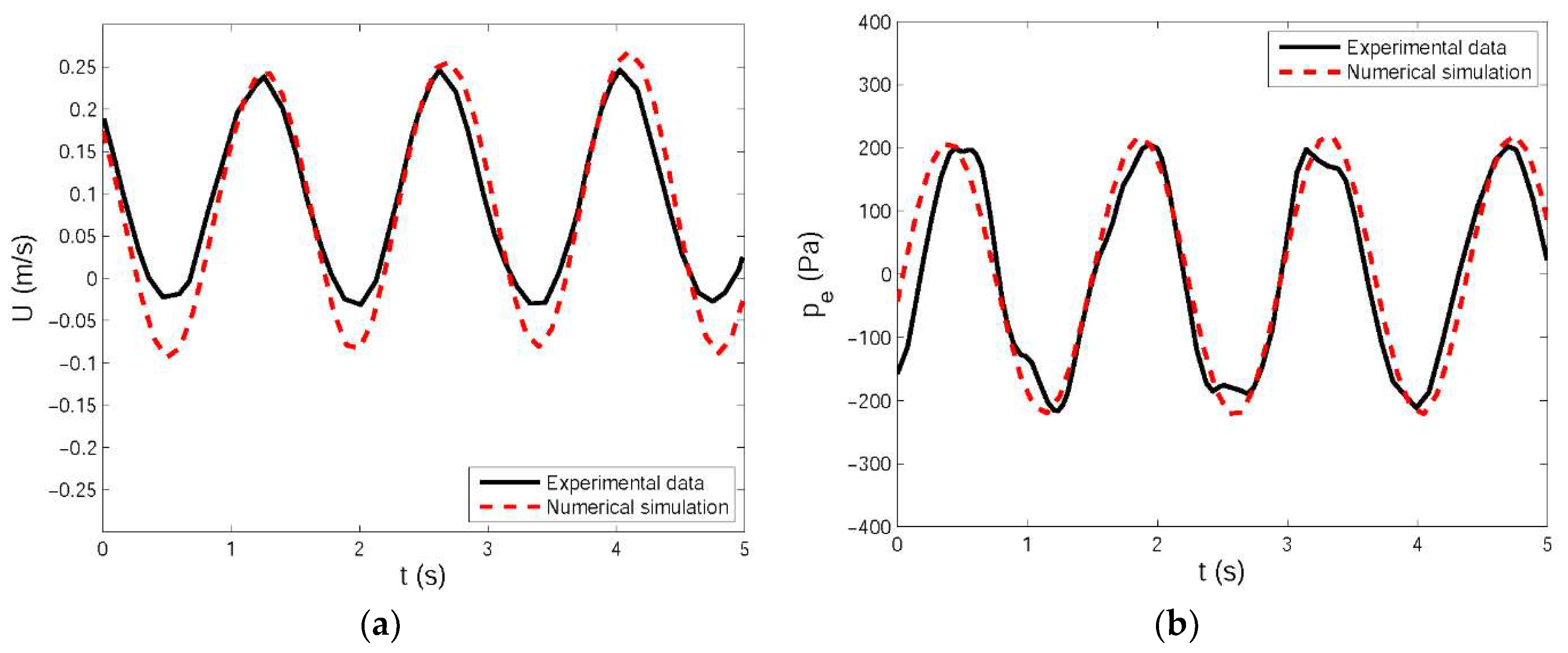
The results with various current velocities are shown in Figure 8, Figure 9 and Figure 10. The flow velocity represents the fluid particle velocity located at 0.2 m above the seabed surface. Differences between the present model and the experimental data are observed because the wave height generated in the experiment cannot be exactly the same as the value expected. Furthermore, the discrepancy occurs close to the wave crest and trough, which may be induced by the transformation of the linear wave profile into a nonlinear wave during propagation from the wave generator to the flume end. The phase of the pore pressure in porous sediments closely corresponds to the phase of the progressive wave above it. In spite of this, there is a trend toward overall agreement with the experimental data. Note, that in these cases, both the water wave (with current) and the seabed response are fully integrated into coupled FEM codes to simulate the wave (current)-seabed interaction, demonstrating the efficiency and ability of the present model when estimating the pore pressure in complex and multi-phase marine deposits.
4. Model Application
Under cyclic wave loading, pore pressure varies extensively in the seabed. When wave-induced pore pressure exceeds a certain limit, soil liquefaction occurs. The following liquefaction criterion could be used to estimate the liquefaction potential:
where and are the unit weights of the seabed soil and water, respectively, and and are the wave-induced pore pressure in the seabed and the wave-induced pressure on the seabed surface, respectively.
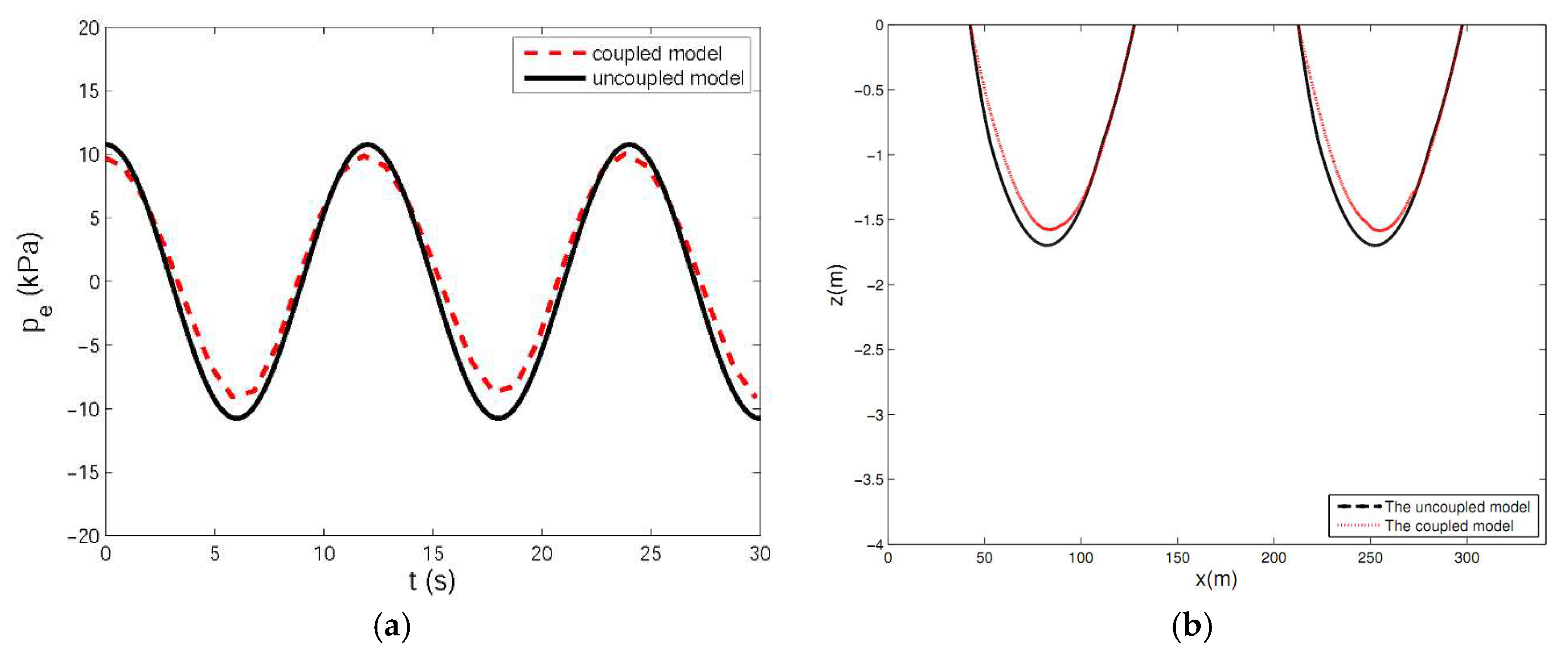
To examine the difference between the coupled and uncoupled models on the wave-induced soil response in marine sediments, the development of wave-induced pore pressure and liquefaction depth is presented in Figure 11. To control other variables (like plasticity) that may affect the liquefaction area, both models only apply the elastic theory to modelling the seabed response. Other parameters are shown in Table 1.
As shown in Figure 11, both wave-induced pore pressure and liquefaction depth in the coupled model are smaller than that in the uncoupled or semi-coupled model. Considering that the seabed surface displacement induced by water waves may alter the flow field in the wave generation model, which was not considered in the previous one-way model, the water pressure acting on the seabed suffers decreases due to the seabed surface motion. Therefore, the soil response may be slightly smaller than in the uncoupled model, and so may the liquefaction area. The results imply that the previous one-way or semi-coupled models ignored the attenuation effect of the porous seabed on water waves, resulting in an over-estimation of the wave-induced pore pressure within marine sediments. Otherwise, a physical scale model would be necessary to verify the results from the traditional uncoupled numerical model. Although, in this case, the discrepancy did not seem significant, its effects may be amplified when evaluating seabed liquefaction in the vicinity of marine structures. This conclusion would be of practical value when applying the traditional one-way model to evaluate the soil response during water wave loading.
5. Conclusions
In this paper, a coupled research method for solving wave-seabed interaction problem was presented. Revised RANS equations were employed to govern the ocean wave and the porous fluid in the seabed, while poro-elastoplastic equations were used to describe the mechanical response of the seabed under dynamic wave loading. The coupled numerical model was validated by comparison with an analytical solution (wave module) and experimental data (seabed module) in the literature. Overall, the consistency between the proposed model and the experimental data illustrated the capacity of predicting the response of the soil due to wave loading.
The major advantages of the coupled model include: (1) The wave and seabed models are coupled in the same platform (COMSOL Multiphysics) and all the equations are solved simultaneously; (2) the wave model can be used to simulate not only small amplitude waves but also large waves and nonlinear waves; (3) the elastoplastic model may be more precise when the plasticity of soil cannot be ignored, which is usually important for offshore deposits; and (4) the coupled model could be used for more complex situations such as the wave-seabed-structure interaction.
This paper presented the basic theory of a coupling model and compared it with the data available in the literature. The wave-seabed interaction with a marine structure, such as a pipeline or breakwater, could also be simulated with the present model. Research that focuses on the wave-seabed-structure issue will be carried out in the future.
Author Contributions
C.L. conducted the numerical analysis and write the paper. D.J. and Y.G. motivated this study with good and workable idea. Z.L. helped to build the wave maker in the software. And Q.Z. did the literature review for this paper.
Acknowledgments
The authors are grateful for the support from National Natural Science Foundation of China (Grant Nos. 41602282, 51678360 and 41727802)
Conflicts of Interest
The authors declare no conflicts of interest
Nomenclature
| Symbol | Description | Units |
| ui | Fluid velocity | [m/s] |
| xi | Coordinate | [m] |
| t | Time | [s] |
| Fluid density | [kg/m3] | |
| p | Fluid pressure | [N/m2] |
| gi | Gravitational force | [m/s2] |
| Viscous stress tensor | [N/m2] | |
| Source Region | [-] | |
| Si | Momentum source function | [m/s2] |
| Angular frequency | [/s] | |
| k | Wave number | [/m] |
| Wave obliquity | [1] | |
| Wave amplitude | [m] | |
| L | Wavelength | [m] |
| C | Wave velocity | [m/s] |
| Free surface elevation | [m] | |
| pe | Wave-induce pore pressure | [Pa] |
| Oscillatory pore pressure | [Pa] | |
| Residual pore pressure | [Pa] | |
| Unite weight of water | [N/m3] | |
| ns | Soil Porosity | [1] |
| Volume strain | [1] | |
| Compressibility of pore fluid | [/Pa] | |
| us, ws | Soil displacements | [m] |
| Kw | True elasticity modulus of pore water | [Pa] |
| Pw0 | Absolute water pressure | [Pa] |
| S | Seabed degree of saturation | [1] |
| Total stress | [Pa] | |
| Effective stress | [Pa] | |
| Kronecker delta | [1] | |
| G | Shear modulus | [Pa] |
| Poisson’s ratio | [1] | |
| Kv | Bulk modulus of soil | [Pa] |
| Plastic volumetric strain | [1] | |
| R | Material parameters | [1] |
| Cyclic stress ratio | [1] | |
| Maximum amplitude of shear stress | [Pa] | |
| Initial effective stress in vertical direction | [Pa] | |
| Wave pressure on seabed surface | [Pa] | |
| Shear stress at the seabed surface | [Pa] | |
| h | Seabed thickness | [m] |
| Turbulent dissipation rate | [1] | |
| Kinetic viscosity | [kg/m/s] | |
| Eddy viscosity | [kg/m/s] |
References
- Damgaard, J.S.; Sumer, B.M.; Teh, T.C.; Palmer, A.C.; Foray, P.; Osorio, D. Guidelines for Pipeline On-Bottom Stability on Liquefied Noncohesive Seabeds. J. Waterw. Port Coast. Ocean Eng. 2006, 132, 300–309. [Google Scholar] [CrossRef]
- De Groot, M.B.; Kudella, M.; Meijers, P.; Oumeraci, H. Liquefaction Phenomena underneath Marine Gravity Structures Subjected to Wave Loads. J. Waterw. Port Coast. Ocean Eng. 2006, 132, 325–335. [Google Scholar] [CrossRef]
- Mutlu, S.B. Liquefaction Around Marine Structures (With Cd-rom); World Scientific: Hackensack, NJ, USA, 2014; ISBN 9814603732. [Google Scholar]
- Maljaars, P.; Bronswijk, L.; Windt, J.; Grasso, N.; Kaminski, M. Experimental Validation of Fluid–Structure Interaction Computations of Flexible Composite Propellers in Open Water Conditions Using BEM-FEM and RANS-FEM Methods. J. Mar. Sci. Eng. 2018, 6, 51. [Google Scholar] [CrossRef]
- Chiang, C.Y.; Pironneau, O.; Sheu, T.; Thiriet, M. Numerical Study of a 3D Eulerian Monolithic Formulation for Incompressible Fluid-Structures Systems. Fluids 2017, 2, 34. [Google Scholar] [CrossRef]
- Devolder, B.; Stratigaki, V.; Troch, P.; Rauwoens, P. CFD Simulations of Floating Point Absorber Wave Energy Converter Arrays Subjected to Regular Waves. Energies 2018, 11, 641. [Google Scholar] [CrossRef]
- Hsu, J.R.C.; Jeng, D.S. Wave-induced soil response in an unsaturated anisotropic seabed of finite thickness. Int. J. Numer. Anal. Methods Geomech. 1994, 18, 785–807. [Google Scholar] [CrossRef]
- Ulker, M.B.C.; Rahman, M.S.; Jeng, D.S. Wave-induced response of seabed: Various formulations and their applicability. Appl. Ocean Res. 2009, 31, 12–24. [Google Scholar] [CrossRef]
- Tong, D.; Liao, C.; Jeng, D.-S.; Zhang, L.; Wang, J.; Chen, L. Three-dimensional modeling of wave-structure-seabed interaction around twin-pile group. Ocean Eng. 2017, 145, 416–429. [Google Scholar] [CrossRef]
- Zhang, Q.; Zhou, X.; Wang, J.; Guo, J. Wave-induced seabed response around an offshore pile foundation platform. Ocean Eng. 2017, 130, 567–582. [Google Scholar] [CrossRef]
- Chen, C.Y.; Hsu, J.R.C. Interaction between internal waves and a permeable seabed. Ocean Eng. 2005, 32, 587–621. [Google Scholar] [CrossRef]
- Jeng, D.S.; Ye, J.H.; Zhang, J.S.; Liu, P.L.F. An integrated model for the wave-induced seabed response around marine structures: Model verifications and applications. Coast. Eng. 2013, 72, 1–19. [Google Scholar] [CrossRef]
- Ye, J.; Jeng, D.; Wang, R.; Zhu, C. Validation of a 2-D semi-coupled numerical model for fluid-structure-seabed interaction. J. Fluids Struct. 2013, 42, 333–357. [Google Scholar] [CrossRef]
- Hur, D.-S.; Kim, C.-H.; Yoon, J.-S. Numerical study on the interaction among a nonlinear wave, composite breakwater and sandy seabed. Coast. Eng. 2010, 57, 917–930. [Google Scholar] [CrossRef]
- Choi, J.; Yoon, S.B. Numerical simulations using momentum source wave-maker applied to RANS equation model. Coast. Eng. 2009, 56, 1043–1060. [Google Scholar] [CrossRef]
- Israeli, M.; Orszag, S.A. Approximation of radiation boundary conditions. J. Comput. Phys. 1981, 41, 115–135. [Google Scholar] [CrossRef]
- Comsol Multiphysics. Comsol Multiphysics User’s Guide; COMSOL Inc.: Burlington, MA, USA, 2010; ISBN 1781273332. [Google Scholar]
- Lin, P.; Liu, P.L.-F. Internal Wave-Maker for Navier-Stokes Equations Models. J. Waterw. Port Coast. Ocean Eng. 1999, 125, 207–215. [Google Scholar] [CrossRef]
- Wei, G.; Kirby, J.T.; Sinha, A. Generation of waves in Boussinesq models using a source function method. Coast. Eng. 1999, 36, 271–299. [Google Scholar] [CrossRef] [Green Version]
- Sassa, S.; Sekiguchi, H. Wave-induced liquefaction of beds of sand in a centrifuge. Geotech. 1999, 49, 621–638. [Google Scholar] [CrossRef]
- Biot, M.A. General theory of three-dimensional consolidation. J. Appl. Phys. 1941, 12, 155–164. [Google Scholar] [CrossRef]
- Yamamoto, T.; Koning, H.L.; Sellmeijer, H.; Hijum, E.V. On the response of a poro-elastic bed to water waves. J. Fluid Mech. 1978, 87, 193–206. [Google Scholar] [CrossRef]
- Liao, C.C.; Zhao, H.; Jeng, D.-S. Poro-Elasto-Plastic Model for the Wave-Induced Liquefaction. J. Offshore Mech. Arct. Eng. 2015, 137, 42001. [Google Scholar] [CrossRef]
- Ye, J.; Jeng, D.S. Effects of bottom shear stresses on the wave-induced dynamic response in a porous seabed: PORO-WSSI (shear) model. Acta Mech. Sin. 2011, 27, 898–910. [Google Scholar] [CrossRef]
- Liu, B.; Jeng, D.S.; Ye, G.L.; Yang, B. Laboratory study for pore pressures in sandy deposit under wave loading. Ocean Eng. 2015, 106, 207–219. [Google Scholar] [CrossRef]
- Sekiguchi, H.; Kita, K.; Okamoto, O. Response of Poro-Elastoplastic Beds to Standing Waves. Soils Found. 1995, 35, 31–42. [Google Scholar] [CrossRef]
- Qi, W.G.; Gao, F.P. Physical modeling of local scour development around a large-diameter monopile in combined waves and current. Coast. Eng. 2014, 83, 72–81. [Google Scholar] [CrossRef]
Figure 1.
Sketch of wave (current)-seabed interaction.

Figure 2.
Comparison of (a) free surface elevation and (b) water pressure between the coupled model and the analytical solution. The small amplitude wave theory is applied for the analytical solution.
Figure 2.
Comparison of (a) free surface elevation and (b) water pressure between the coupled model and the analytical solution. The small amplitude wave theory is applied for the analytical solution.

Figure 3.
Schematic diagram of one-dimensional cylinder equipment (adapted from [25]).
Figure 3.
Schematic diagram of one-dimensional cylinder equipment (adapted from [25]).
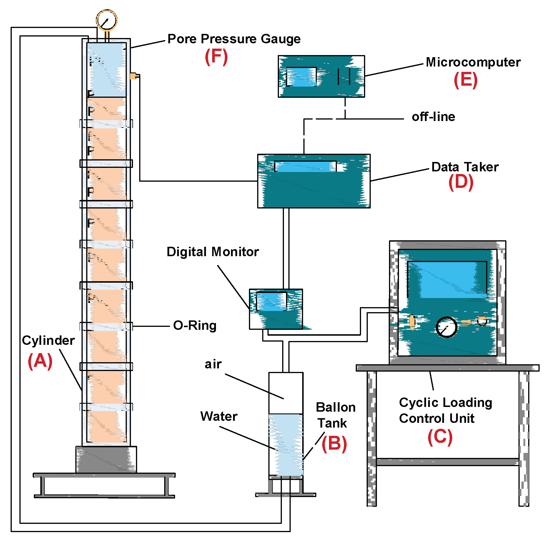
Figure 4.
Comparison of oscillatory pore pressure with one-dimensional experimental data. The experimental data include pore pressure records of ten gauges (P0 to P9).
Figure 4.
Comparison of oscillatory pore pressure with one-dimensional experimental data. The experimental data include pore pressure records of ten gauges (P0 to P9).

Figure 5.
Cross-section of two-dimensional centrifuge equipment (units are mm).
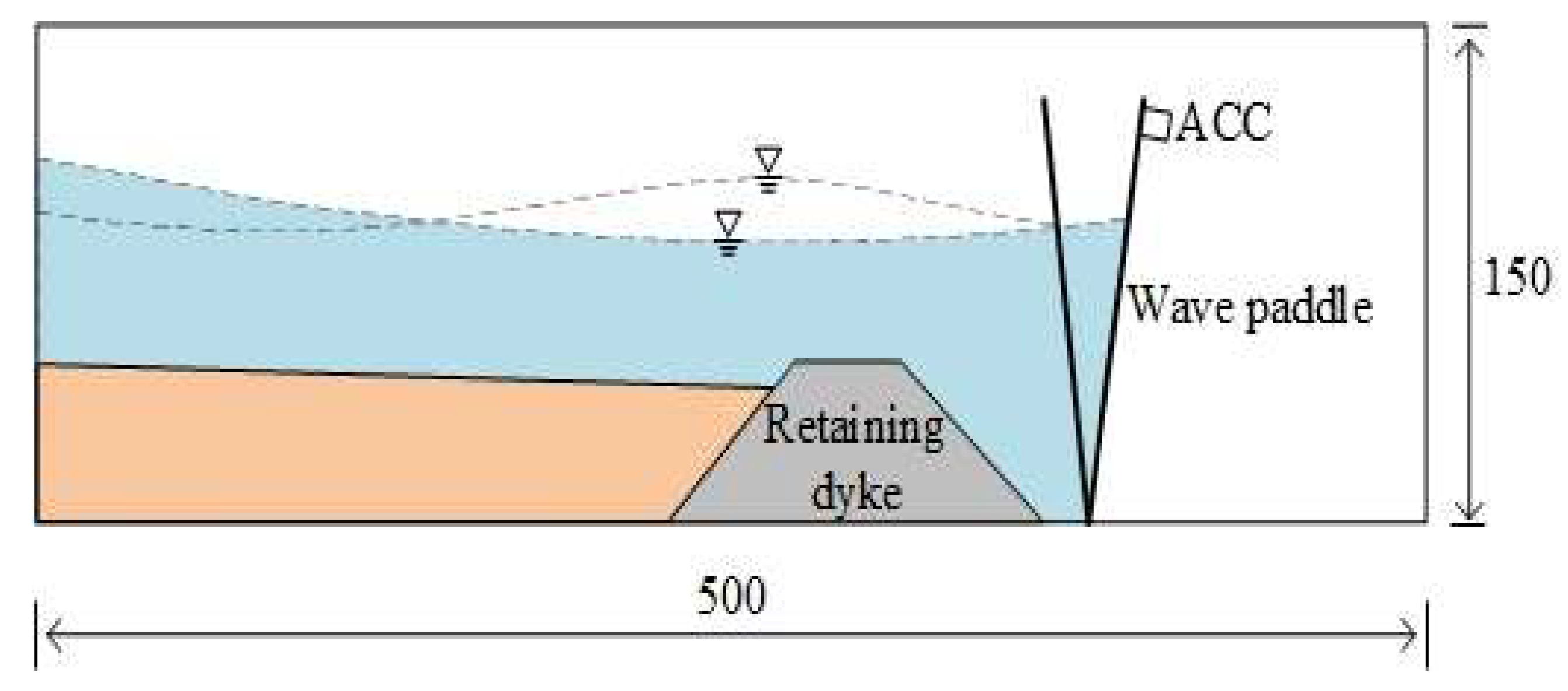
Figure 6.
Comparison of residual pore pressure with standing wave centrifugal test data [20]. Time history of pore pressure is from the soil element at elevation z/h = 0.25.
Figure 6.
Comparison of residual pore pressure with standing wave centrifugal test data [20]. Time history of pore pressure is from the soil element at elevation z/h = 0.25.
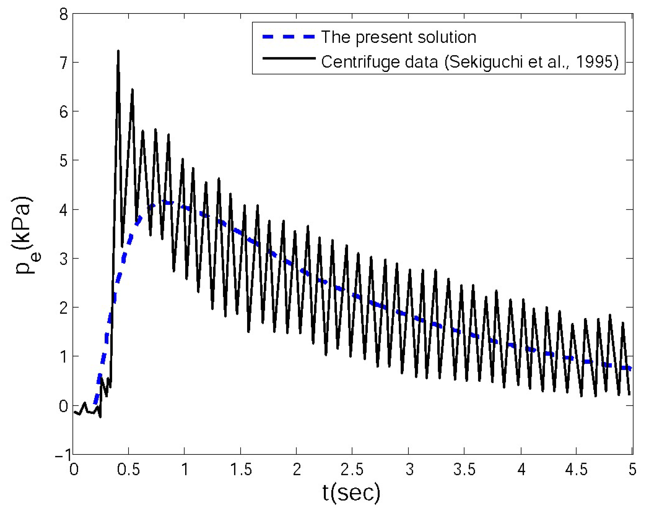
Figure 7.
Schematic diagram of three-dimensional water flume system (adapted from [27]). (Units are m).
Figure 7.
Schematic diagram of three-dimensional water flume system (adapted from [27]). (Units are m).

Figure 8.
Comparison of (a) flow velocity and (b) pore pressure between the present coupled model and experimental data (U0 = −0.1 m/s). The flow velocity represents the fluid velocity at 0.2 m above the seabed surface and pore pressure is from the soil element that was located at point C in Figure 7.
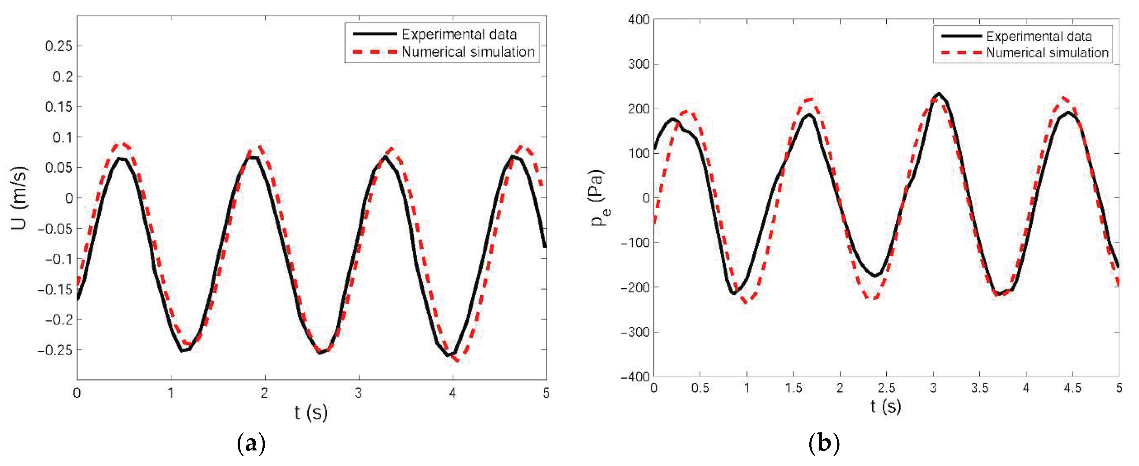
Figure 9.
Comparison of (a) flow velocity and (b) pore pressure between the present coupled model and experimental data (U0 = 0 m/s). The flow velocity represents the fluid velocity at 0.2 m above the seabed surface and pore pressure is from the soil element that was located at point C in Figure 7.
Figure 9.
Comparison of (a) flow velocity and (b) pore pressure between the present coupled model and experimental data (U0 = 0 m/s). The flow velocity represents the fluid velocity at 0.2 m above the seabed surface and pore pressure is from the soil element that was located at point C in Figure 7.

Figure 10.
Comparison of (a) flow velocity and (b) pore pressure between the present coupled model and experimental data (U0 = +0.1 m/s). The flow velocity represents the fluid velocity at 0.2 m above the seabed surface and pore pressure is from the soil element that was located at point C in Figure 7.

Figure 11.
Comparison of (a) pore pressure and (b) liquefaction depth within the seabed between coupled and uncoupled models.
Figure 11.
Comparison of (a) pore pressure and (b) liquefaction depth within the seabed between coupled and uncoupled models.


Table 1.
Input data for application of present model.
| Wave Characteristics | Value | Soil characteristics | Value |
|---|---|---|---|
| Wave period (T) | 12.0 s | Permeability (K) | 1.0 × 10⁻⁴ m/s |
| Porosity (ne) | 0.30 | ||
| Wave length (H) | 170.0 m | Shear modulus (G) | 1.0 × 10⁷ N/m2 |
| Thickness (h) | ∞ m | ||
| Water depth (d) | 30.0 m | Poisson’s ratio (μ) | 0.35 |
| Degree of saturation (S) | 1 | ||
| Wave amplitude (η) | 2.5 m |
© 2018 by the authors. Licensee MDPI, Basel, Switzerland. This article is an open access article distributed under the terms and conditions of the Creative Commons Attribution (CC BY) license (http://creativecommons.org/licenses/by/4.0/).
Share and Cite
MDPI and ACS Style
Liao, C.; Jeng, D.; Lin, Z.; Guo, Y.; Zhang, Q. Wave (Current)-Induced Pore Pressure in Offshore Deposits: A Coupled Finite Element Model. J. Mar. Sci. Eng. 2018, 6, 83. https://doi.org/10.3390/jmse6030083
AMA Style
Liao C, Jeng D, Lin Z, Guo Y, Zhang Q. Wave (Current)-Induced Pore Pressure in Offshore Deposits: A Coupled Finite Element Model. Journal of Marine Science and Engineering. 2018; 6(3):83. https://doi.org/10.3390/jmse6030083
Chicago/Turabian StyleLiao, Chencong, Dongsheng Jeng, Zaibin Lin, Yakun Guo, and Qi Zhang. 2018. "Wave (Current)-Induced Pore Pressure in Offshore Deposits: A Coupled Finite Element Model" Journal of Marine Science and Engineering 6, no. 3: 83. https://doi.org/10.3390/jmse6030083
Note that from the first issue of 2016, this journal uses article numbers instead of page numbers. See further details here.