Failure of Grass Covered Flood Defences with Roads on Top Due to Wave Overtopping: A Probabilistic Assessment Method

Abstract

Hard structures, i.e., roads, are commonly found over flood defences, such as dikes, in order to ensure access and connectivity between flood protected areas. Several climate change future scenario studies have concluded that flood defences will be required to withstand more severe storms than the ones used for their original design. Therefore, this paper presents a probabilistic methodology to assess the effect of a road on top of a dike: it gives the failure probability of the grass cover due to wave overtopping over a wide range of design storms. The methodology was developed by building two different dike configurations in computational fluid dynamics Navier–Stokes solution software; one with a road on top and one without a road. Both models were validated with experimental data collected from field-scale experiments. Later, both models were used to produce data sets for training simpler and faster emulators. These emulators were coupled to a simplified erosion model which allowed testing storm scenarios which resulted in local scouring conditioned statistical failure probabilities. From these results it was estimated that the dike with a road has higher probabilities (5 × 10⁻⁵ > P_f >1 × 10⁻⁴) of failure than a dike without a road (P_f < 1 × 10⁻⁶) if realistic grass quality spatial distributions were assumed. The coupled emulator-erosion model was able to yield realistic probabilities, given all the uncertainties in the modelling process and it seems to be a promising tool for quantifying grass cover erosion failure.

1. Introduction

Structural embedment of roads on top of dikes will generate stability effects in the flood defence during normal operation and during a flood event [1]. Yet, these effects are not explicitly considered in the current probabilistic assessment methods. It is expected that climate change increases sea level rise and that it will affect the wave climate around the world [2,3]. For rivers, extreme water levels occur more frequently as shown for the River Rhine basin [4], for example. Such climate change effects increase the risk of flooding of low lying, highly populated areas around world [5,6]. In the last decades, flood defence design has moved towards a risk-based approach [7,8] in which it is possible to express the design parameters uncertainty as probabilistic distributions [8]. Such methods allow inclusion of the expected future effects due to climate change as modifications in the parameter statistical distributions. Nevertheless, there is a lack of methods for assessing non-convectional flood defences so that their interaction effects are also captured and reflected in the estimated failure probabilities [1]. In case of grass covered dikes the failure mechanism known as wave overtopping is influenced by the presence of non-water retaining functions [1]. This failure mechanism consists in the intermittent surpass of water excess volumes over the dike derived from the ‘attacking’ waves during a storm. Only the waves that surpass the crest height will overtop and ‘attack’ the landward slope of the dike, potentially eroding the cover until an eventual dike breach.

For dike cover erosion assessment, reliability methods based on partial safety factors validated by a fully probabilistic Monte Carlo method are available [9]. These methods are based on the classical overtopping approach of defining dike safety based on an allowable overtopping discharge $q_{max}$ [m³/s/m]. Other studies concluded that overtopping erosion is better estimated from individual wave overtopping volumes $V$ [m³/m] [10,11,12,13]. In Ref. [14], three different erosion predictors (velocity excess, shear stress excess, and work excess) were tested for calculating the scour depths per wave volume and they found that work excess was the best predictor. Simultaneously, the cumulative overload method [15] was developed which relies on the shear stress principle, using the total overtopping duration per wave as input while acknowledging that the “real” erosion time per wave may be shorter. Additional research [16,17] allows inclusion of the effects of obstacles and transitions in both the hydraulic load and resistance terms in the form of calibration coefficients for the cumulative overload method from Ref. [15].

With respect to the grass cover resistance, a conceptual geo-mechanical approach [18] describes the physical process of grass cover erosion based on the vertical and horizontal stresses that act upon a turf element model. In addition, two main studies [19,20] recommended grass and soil quality values expressed in terms of their erodibility rates. Based on these studies and concepts, Ref. [21] aimed to determine the grass cover failure of conventional dikes in terms of probabilities, while considering the spatial distribution of grass quality. The method used in this last study is fully probabilistic and could be adapted to more complex dike profiles. Nevertheless, it relies on empirical formulas for estimating the water depths and flow velocities on top of the crest and along the landside slope. These empirical formulas [22] simplified the estimation of water depth and flow velocity for the design of sea dikes by proving a set of equations. More holistic approaches [23,24] are available for including the effects of bottom irregularities in the flow. Both studies used one dimensional (1D) models, which allowed to simulate the time-dependent erosion process of a grass covered coastal dike. Yet, both models estimate the exerted bottom shear stresses as a function of uniform flow models, such as Chezy or Manning, which are only applicable for smooth bed slope transitions. If abrupt bottom slope variations occur, the vertical velocity distribution tends to have a larger variability [25], thereby violating the uniform flow assumption. This variability might result in more turbulent flows, higher energy dissipation and hence less accurate bed shear stress estimations. The work presented in Ref. [26] used a more detailed computational fluid dynamics (CFD) model and showed that the presence of a road leads to higher scour depths in places with little to non-existent grass cover. In this paper, we extend the deterministic CFD approach of Ref. [26] towards a fully probabilistic assessment method for failure of the grass cover due to wave overtopping erosion.

Emulation of detailed models is as an efficient way to reduce computational times, for implementation in probabilistic failure studies. Emulation consists of building a computationally inexpensive model and training it with data sets generated from the input-output data sets obtained from more complex models [27,28]. Hydrodynamic model emulation has proven to be a powerful tool for water level predictions while improving the calculation speed significantly [29,30]. Also, for the reliability assessment of flood defences, emulation has already been implemented for other failure mechanisms, such as backward piping erosion [31,32,33]. For wave overtopping, [34] used the results of 10,000 physical model tests of different types of coastal defences to train a neural network.

The aim of this study was to develop an emulator-based dike failure assessment methodology for estimating the effects of a road over the crest including the spatial variation of the grass quality in the failure probability of the grass cover. This failure is estimated as a function of a storm surge wave overtopping event composed of a set of single overtopped water volumes due to wind generated gravity waves, which flow over the dike profile. The methodology was based on two different CFD transient models; one with a road on top [35] and one fully covered with grass. The research question we are answering in this paper is: What is the effect of a road on the grass cover failure probability of a dike due to overtopping waves?

The article is composed of 6 main sections. Section 2 explains the theoretical background of the shear stress excess (${\rm T}$). Section 3 explains the experiment in Millingen from which the collected data was used for construction and calibration of the models. Section 4 presents a detailed explanation of the steps of the developed methodology and its correspondent assumptions. Section 5 and Section 6 present the results and discussion and Section 7 gives the conclusions to highlight the major findings.

2. Theoretical Background

Wave overtopping erosion is a transient process in which tensile and shear stresses are exerted along the dike grass cover over time because of the overtopped water volume’s momentum. While the erosion is generated by one single wave, it has been observed that failure of the dike cover is mostly achieved by the overtopping of numerous waves during a storm event [12]. The time span in which erosion caused by a single wave takes place at a specific location is in the order of seconds [26] and it is termed total wave overtopping time ($t_{total}$). This duration differs from wave to wave depending on its volume, flow depth, and flow velocity and it is spatially influenced by the surface irregularities and bottom slope. If the generated stresses exceed the mechanical resistance of the grass cover elements (e.g., grass leaves, roots, substrate), erosion occurs by pulling, scouring, and flushing the eroded material downstream.

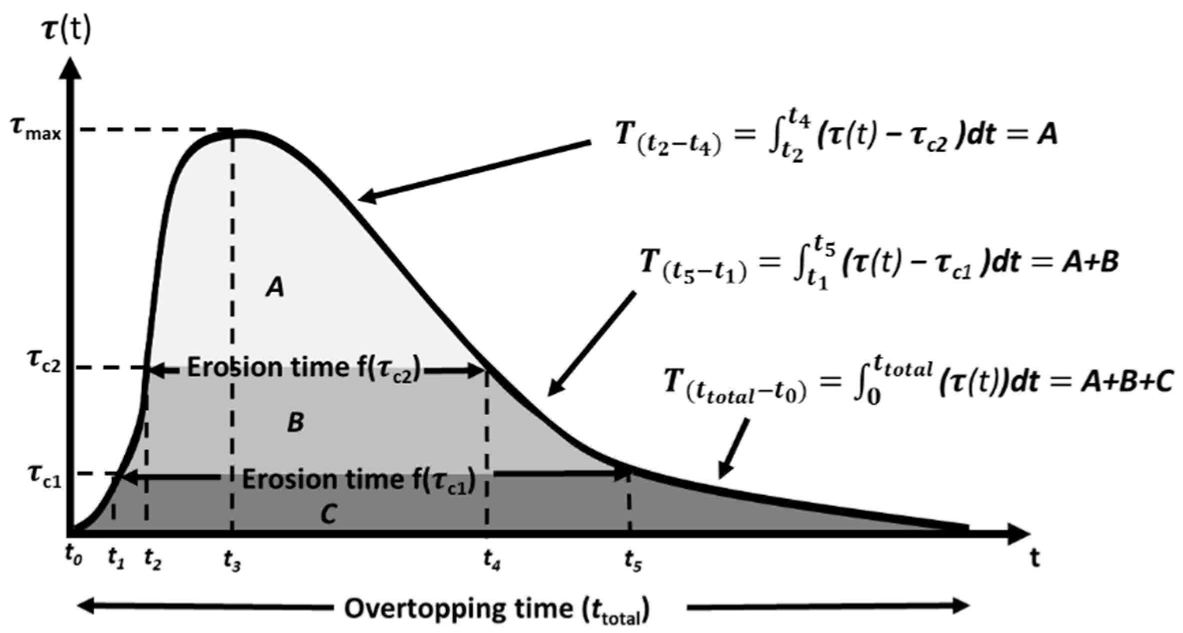
2.1. Shear Stress Excess (${\rm T}$)

Most of the overtopping scour erosion methods are based on definitions of critical threshold values for average overtopping discharges in steady flow conditions [14]. For combined grass and soil covers, the scour threshold can also be defined by a critical shear stress ${\tau }_c$, which depends on the grass cover quality [19]. This value only represents the threshold which defines if scouring occurs or not. To include two other important scour characteristics (erosion rate and real erosion duration), the time dependent shear stress excess [N∙s/m²] concept from [36] was adopted in the present study. It represents the surplus of shear stress during the period of time in which erosion occurs. Only during this period does erosion take place. This implies that for larger values of ${\tau }_c$, the difference between the total overtopping duration ($t_{total}$) and the real erosion time span (e.g., $f\left({\tau }_{c2}\right)=t_4-t_2$ in Figure 1) is significant. The value of ${\rm T}$ is calculated for a given location along the profile as the integral of the bottom shear stress function $\tau \left(t\right)$ minus the critical erosion stress threshold ${\tau }_c$, over the erosion time span (e.g., area A for time span $t_4-t_2$ and ${\tau }_{c2}$ in Figure 1). A lower value of ${\tau }_c$ represents lower resistance to erosion and implies a longer time span of erosion and a greater.

The fact that the erosion time span (t_i+1 − t_i) and the total wave overtopping duration time ($t_{total}$) differs may have a significant influence on the estimated erosion was acknowledged in Ref. [37], who included the “real” erosion excess time by assuming a triangular shape of the wave overtopping discharge hydrograph. However, this assumption may be too general for representing the shear stress excess over a highly irregular bottom profile. The overtopping integration bounds (t_i+1 and t_i) vary between locations due to the presence of bottom irregularities which may either accelerate or decelerate the overtopping flows. In addition, their values are also determined by the value of ${\tau }_c$ (See Figure 1).

2.2. Erosion Model as a Function of ${\rm T}$

The erosion model used in the present study is derived from the time dependent mass erosion rate equation for cohesive soils presented in Ref. [38] as:

$$\frac{dm}{dt}+M_p\frac{\left(\tau -{\tau }_c\right)}{{\tau }_c}=0$$

(1)

In which $M_p$ [kg/(m²s)] corresponds to the characteristic soil mass transport coefficient, $\frac{dm}{dt}$ corresponds to the mass transport rate in time, $\tau$ [N/m²] corresponds to the exerted bottom shear stress, and ${\tau }_c$ [N/m²] corresponds to the critical shear stress threshold.

According to [36], an overall erosional strength parameter $C_E$ [m/s⁻¹] for soil and grass together was derived [19] as:

$$C_E\equiv \frac{M_p}{{\tau }_c}$$

(2)

Note that the $C_E$ parameter is directly proportional to $M_p$ and inversely proportional to ${\tau }_c$. Based on this equivalence and by dividing Equation (1) by the dike cover relative density per unit of width ($\rho {’}_{cover}$ [kg/m²]), the erosion rate at any specific location for a unitary width of dike can be expressed as:

$$\frac{d\epsilon }{dt}+\frac{C_E}{\rho {’}_{cover}}\left(\tau \left(t\right)-{\tau }_c\right)=0$$

(3)

Since $C_E$ or $\rho {’}_{cover}$ are independent of time, the scour depth ($\epsilon$) in a particular location can be calculated by integrating Equation (3) as:

$$-\underset{x_i}{\overset{x_{i+1}}{\int }}d\epsilon =\frac{C_E}{\rho {’}_{cover}}\underset{t_i}{\overset{t_{i+1}}{\int }}\left(\tau \left(t\right)-{\tau }_c\right)dt$$

(4)

The integral on the right side of Equation (4) represents the ${\rm T}$ value for a given ${\tau }_c$ for a single overtopped wave. The integral bounds of the right-side integral are defined by the specific moments in time where $\tau \left(t\right)\ge {\tau }_c$, as erosion will occur during this condition (Figure 1). The integrand bound $x_i$ represents the initial bottom elevation before the scouring process and $x_{i+1}$ the resultant bottom elevation after the scouring process. This model includes the time-dependent variability of the shear stress, but it only estimates the erosion process as a function of the bottom shear stresses. The vertical tensile resistance of grass and roots of the grass cover [36] are accounted for in the parameterization by the $C_E$ coefficient. These tensile stresses are described by the turf element method [36] but were too complex to be included in the model. Therefore, the shear stress excess erosion concept presented in Section 2.1 is selected as it requires less input data and allows to use the erodibility value $C_E$ [19]. This simplification makes the implementation more feasible for a probabilistic model as it represents the grass quality and resistance uncertainty in one single stochastic variable.

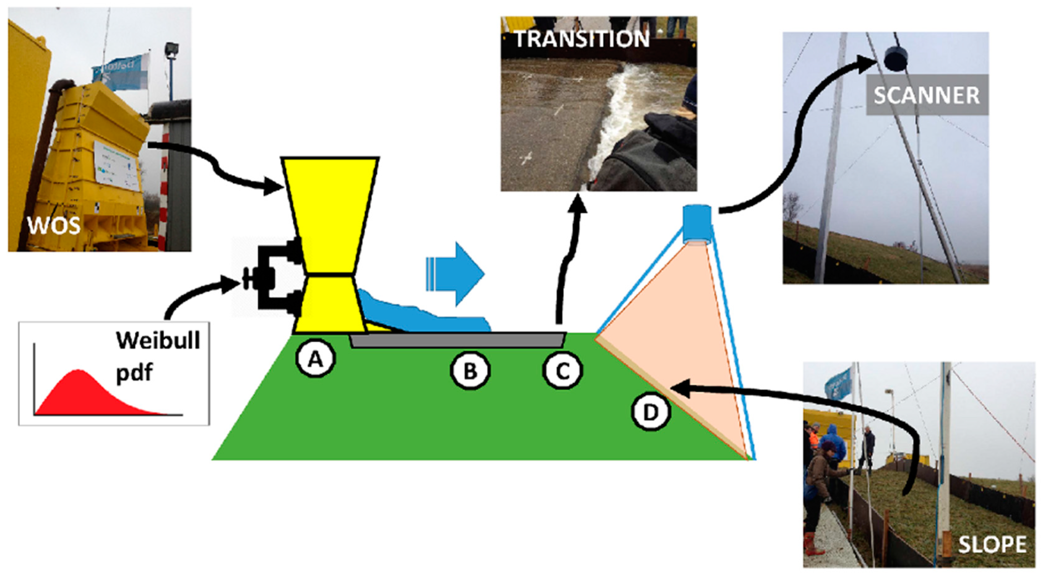
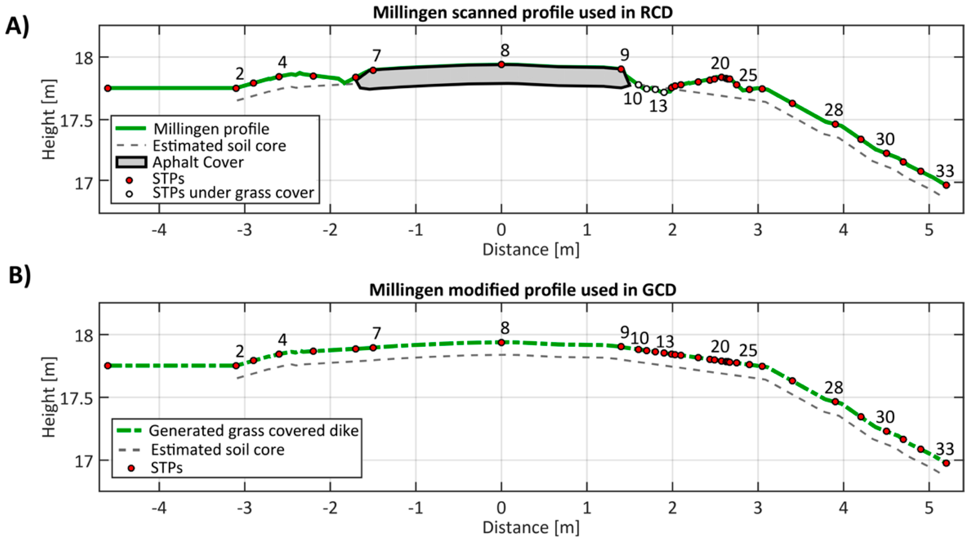
3. Millingen aan de Rijn Wave Overtopping Experiment with a Road on Top

Experiments for wave overtopping were conducted on top of a riverine dike along the river Waal nearby Millingen aan de Rijn (The Netherlands) in February and March of 2013 [39]. Random wave volumes $V$ [m³/m] were released by the wave overtopping simulator (WOS) [15] during a period of time equivalent to the duration of a storm. The WOS was located on top of the crest of the dike close to the riverside vertex (see Figure 2).

For the present study, a storm condition is defined by a crest height ($R_c$ [m]), a water level and the total number of waves $N_w$[-] generated in the foreshore, with significant wave height, $H_s$[m], during the storm duration period $D$[s]. In addition, a storm condition is often characterized by its mean overtopping discharge per unit of width $q_m$[m³/s/m]. This discharge is calculated as the total overtopped volume of water per storm divided by storm duration as shown in Equation (5):

$$q_m=\frac{{\sum }_{j=1}^{j={\mathit{N}}_{ow}}{V}_j}{D}$$

(5)

Note that the same storm event may generate a different $q_m$ depending on the crest level of the dike as only a limited number of wave volumes will overtop the dike $N_{ow}$ [-]. Hence, for this study, a combination of factors (e.g., wave conditions, dike geometry, and roughness) that originate a certain $q_m$ is referred to a storm condition. In the WOS experiment, 10 storm conditions were simulated consecutively. After each simulated storm condition, the dike was scanned using a 3D laser scanner to estimate the scour depths and spatial scouring patterns. This experiment included a road on top of the dike to analyze the effect of transitions on the scouring process due to wave overtopping. The experiment was divided into two parts performed in two adjacent locations. Each test location was 4 m wide with lateral walls that prevented leakage during the tests.

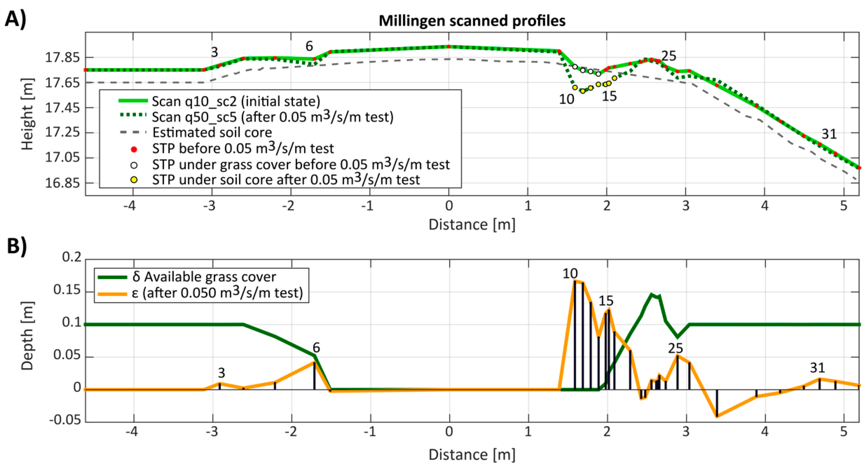
3.1. Millingen Experiment Part I: Scour Measurements

During the first part of the experiment, the WOS was located near the riverside edge of the dike (zone A, Figure 2). From this location, a series of volumes were released during a period of six hours, which is equivalent to the duration of the design storm. The released volumes were randomly sampled following a Weibull distribution which represents the stochastic nature of the waves that overtop the dike during a storm. The former Dutch safety standards, for example [11], allow storm conditions of maximum overtopping discharge $q_{max}$ between 0.001 m³/s/m and 0.01 m³/s/m depending on the dike location, cross sectional design, and materials [12]. The first part of the experiment [39], was conducted for different consecutive storm conditions ($q_m$) as presented in

Table 1. Experimental storm conditions for part I of Millingen experiment.

Experiment Part I
Overtopping Discharge	Interval 1 Interval	Scanning Instant	Profile Scan Label
$q_m$ [m3/s/m]	[min]	[min]	[min]
Initial state	0	0	q0_t0
0.001	72	72	q1_sc1
0.010	180	252	q10_sc1
0.010	180	432	q10_sc2 2
0.050	60	492	q50_sc1
0.050	60	552	q50_sc2
0.050	60	612	q50_sc3
0.050	60	672	q50_sc4
0.050	180	852	q50_sc5 2
0.100	100	952	q100_sc1
0.100	120	1072	q100_sc2

¹ The intervals shows the actual test durations and scanning instant shows the exact moment in which the laser scanning takes place. The ² profiles are used for model the CFD model construction and validation.

.

While the experiment’s durations range from 0 to 3 h for each mean discharge, dikes are often designed for storms that range between 2 and 6 h depending on their boundary conditions. High resolution 3D laser scan images were taken (Figure 2) every 2 h with an accuracy of 2 mm. For some storm conditions, it was necessary to accelerate or decelerate some of the tests due to the WOS pumping constraints and release capacity restrictions. The different storm average discharges are conditioned by the relative position of the crest of the dike with respect to the still water level, the dike geometry, dike cover, and revetment type.

In the initial state profile, already significant damage due to traffic was observed in the transition gap (zone C, Figure 2). This gap increased and propagated landward with each test, as bare soil erodes faster than grass covered soil. Besides this zone, no significant erosion was observed in the grass cover for the 0.001 and 0.010 m³/s/m tests. The scan labels presented in Table 1 include the average overtopping discharge and the scan number of that experiment.

3.2. Millingen Experiment Part II: Flow Depths and Velocity Measurements

The second part of the experiment consisted of measuring flow depth time series and velocity time series of individual overtopping wave volumes along the dike profile. Paddle wheel devices (PW) were used for measuring flow velocities and surfboard meters (SB) for measuring flow depths in 8 locations along the crest and landward slope (see [39] for more details). To exclude the effects on the measurements of the landside road transition and roughness change, a geotextile cover was placed over the transition between the asphalt road and the remaining crest part (Figure 2, zone C). Additionally, the WOS was located directly over the road (Figure 2, zone B), to avoid the induced effects on the flow measurements from the riverside transition. Velocities and depths time series were measured at least two times for wave volumes ($V$) of 0.4, 0.6, 0.8, 1.0, 1.5, 2.0, 2.5, 3.0, 4.0, 5.0, and 5.5 m³/m.

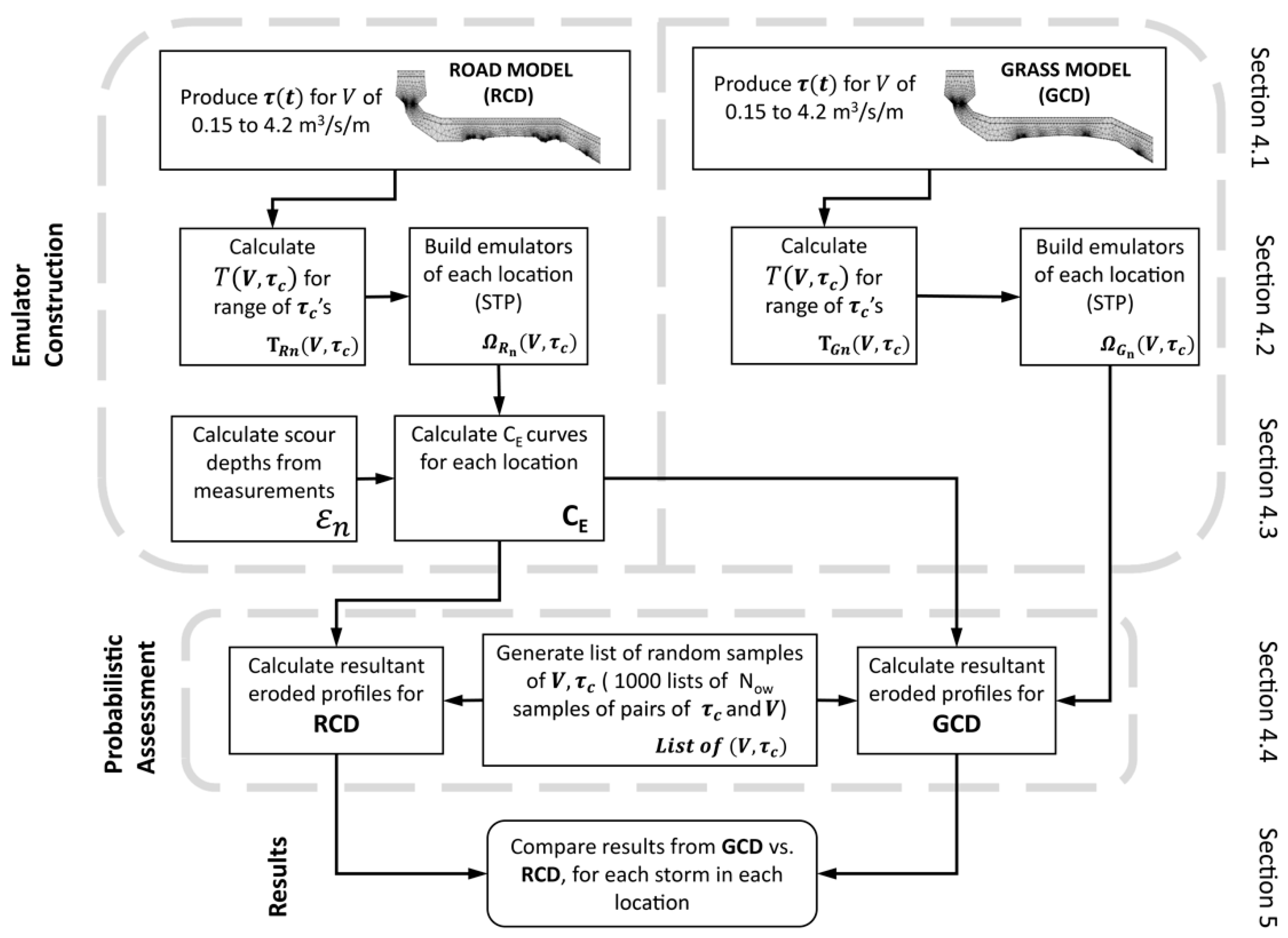
4. Methodology

The complete methodology is divided in 4 steps as shown in the flow chart presented in Figure 3. The first step consists of constructing and validating two CFD models built for producing accurate and detailed time series of bottom shear stresses ($\tau$) along the dike profile as a function of different wave volumes ($V$). The first model includes an asphalt road at the crest of the dike and corresponds to the profile of the Millingen dike initial state scan. This CFD model is referred to as “Road on crest dike” model (RCD). The second model represents the same dike but the road on top was replaced by a smooth grass cover. This CFD model is referred to as “Grass crest dike” model (GCD).

In the second step (Section 4.2) the bottom stress time series ($\tau$) are integrated at each location for different ranges of critical shear stress values (${\tau }_c$). The obtained set of values represent the shear stress excess integral $T$, which are used to build two computationally inexpensive models (emulators) which imitate both CFD models. These emulators are capable of estimating ${\rm T}$ values as a function of combinations of $V$ and ${\tau }_c$ values.

In the third step (Section 4.3), the “grass cover quality” is determined for each location and represented by a $C_E$ function. These functions are calibrated based on the previously built emulators and the scanned profiles of the Millingen experiment part I. One of the main assumptions of the methodology is that the estimated curves are representative for both dike conditions.

Finally, in the fourth step (Section 4.4) the emulators of the RCD and GCD are used to predict the erosion depth at each location along the dike profile, using stochastic input for $V$ and ${\tau }_c$ and the calibrated $C_E$ functions from step 3. This yields a random set of erosion profiles from which the failure probabilities in each location for both the road and grass covered dike are derived for each storm condition ($q_m$). Note that the use of emulators allowed us to reduce the computational times so that crude Monte Carlo simulations could be used that captured the high level of detail of the hydrodynamics instead of using approximate reliability methods such as first order reliability method (FORM) or second order reliability method (SORM) [31].

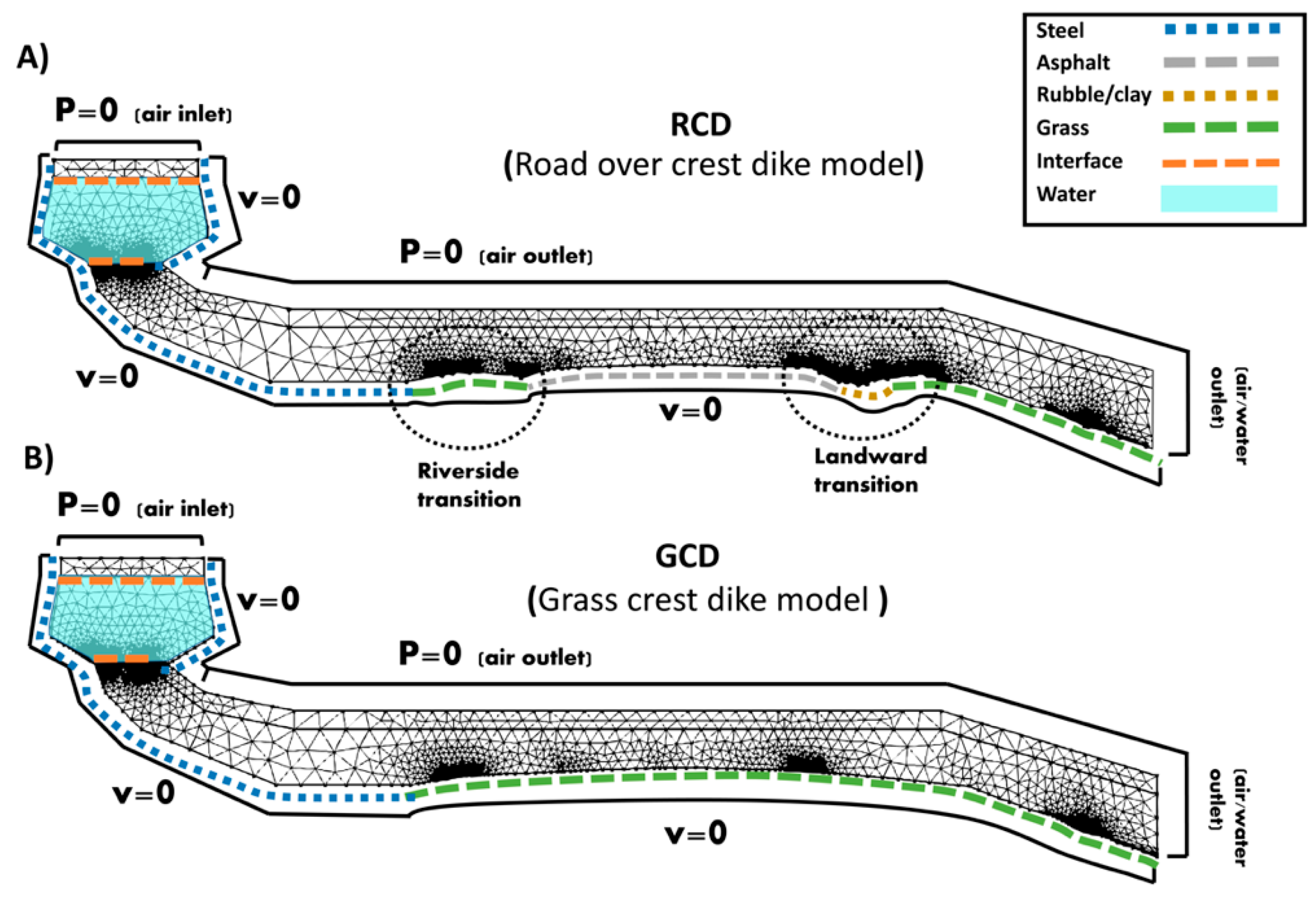
4.1. CFD Models

Detailed two dimensional (2D) CFD Reynolds averaged Navier-Stokes equations (RANS) with k-$\epsilon$ turbulence closure solution models are considered better approximations of flow models where transient bed shear stresses are required with respect to uniform flow-based methods. They simulate turbulent flows for which rapid dissipation of kinematic energy is converted into internal energy in the form of turbulence. The inclusion of turbulence derived effects in the bed shear stresses becomes more important when abrupt geometric bottom changes and local surface roughness variations are present (e.g., RCD bottom profile, see Figure 4).

The RCD and GCD models were built using the COMSOL Multiphysics^® software (COMSOL Inc., Stockholm, Sweden) for solving the 2D RANS k-$\epsilon$ equations for a two-phase field domain (air/water) based on a two equation (k-$\epsilon$) turbulence closure model. This model accounts for turbulence effects by including two additional unknowns; the turbulent kinetic energy ($k$) and the rate of dissipation of kinetic energy ($\epsilon$). Both are used for representing the transfer of momentum inside the flow due to turbulent eddies represented by the eddie viscosity. In addition, a phase field two equation transport approach is used for the interface tracking. For further information of the numerical solution see Ref. [40,41]. Details of the construction of the grid are given in Ref. [35].

The first CFD model (RCD), originally built in Ref. [26,35], was based on the scanned profile obtained as a final condition after the 0.01 m³/s/m experiment (q10_sc2: where q implies the mean overtopping discharge in l/s/m and sc2 refers to scan 2, the first profile scan after the q10 event, see Table 1). This profile includes an asphalt road of 3.1 m width with adjacent eroded transition gaps on each side of approximately 0.5 m each (Figure 4). Additionally, 2.5 m of the landside slope (approx. 1:3) is included in the model domain. For a detailed description of the RCD model setup, the accuracy of the mesh refinement and selected turbulence model we refer to Ref. [26].

A second model (GCD) was built to recreate a dike which could be tested with the same hydrodynamic conditions, but without including the asphalt road and transition gaps present in the original model. This model was built based on the original Millingen experiment dike profile (q10_sc2, Section 3.1), but the transition gaps were removed with a line smoothing procedure. The asphalt cover roughness was replaced by the roughness of grass (Figure 4). The rest of the profile remained unmodified in terms of the original elevation and slopes with respect to the RCD model.

The simulation principle consists of defining a water domain inside the WOS equivalent to the wave volume to be routed and run the model by letting the water to flow free from the domain during 15 s to ensure the whole volume has left the system (besides water retained in concave zones).

Both GCD and RCD models are used for producing the bottom shear stress time series ($\tau \left(t\right)$) along the bottom profile by releasing a certain volume contained in the WOS (see Figure 4). The bottom shear stress is calculated as the product of the flow density times the boundary shear velocity ($u^{*}$) squared. This shear velocity is calculated parallel to the bottom surface which allows to account for the fact that the erosion model was developed assuming a flat bottom. This model also allows one to estimate the tensile stresses in the normal direction of the bottom, but for the present method it is assumed that the erosion is a product of only the tangential shear stresses. The Manning’s roughness coefficients used for both RCD and GCD models were obtained from the measured values reported in Ref. [39]. The steel roughness was used as the calibration value for achieving the measured velocities in the outlet of the WOS. Further information about the calibration may be found in Ref. [1]. The transformation from Manning values ($n$) to equivalent sand roughness ($K_s$) values required as input by the software was done with Ref. [42]:

$$n=0.04K_s{}^{\frac{1}{6}}$$

(6)

The values used for the different boundary material roughness are presented in

Table 2. Roughness coefficients used for both road and crest models from [39].

	$\mathit{n}$	${\mathit{K}}_{\mathit{s}}$ [m]	Source
Surface	[s/m1/3]	[m]	-
Asphalt	0.016	0.0047	[39]
Grass	0.025	0.0680	[39]
Steel	0.017	0.0068	[43]
Rubble/Clay	0.026	0.0670	[43]
Geotextile 1	0.024	0.0660	[44]

¹ This value was not used as input in any of the two CFD models, because its value is similar to grass.

.

Simulations for 0.15, 0.4, 0.7, 1.0, 1.5, 2.5, 3.2, and 4.5 m³/m wave volumes ($V$) were performed in both RCD and GCD models. These values were chosen such that different orders of magnitude could be covered in the emulator training set while also including wave volumes which were measured in the Millingen experiment (0.15, 0.4, 1.0, and 2.5 m³/m) for the CFD models validation (presented in appendices A, B, and C). From each simulation, bottom shear stress time series were generated in 33 different locations along the profiles of both models (Figure 5). From now on these locations are referred to as STP1 until STP33.

These 33 study points (numbered dots in Figure 5) were selected for estimating the erosion depths at the locations where the bottom slope line segment changed significantly with respect to the previous line segment. All 33 STPs are located in the same horizontal position in both RCD and GCD models. The manual smoothing procedure of the RCD profile for generating the GCD profile consisted of placing straight lines between STPs 5 and 7, 9 to 20, and 23 to 26 (Figure 5). According to the field measurements [39,45], the average thickness of the grass cover was around 10 cm (dashed lower line in Figure 5). Points that are below this line in the RCD are located inside the clay zone (e.g., STPS 10 to 13 in the RCD, Figure 5).

The RCD model and its validation are presented in Ref. [35] and Appendix A, Appendix B, and Appendix C of the present study. As the Millingen experiment included a road at the crest, no experimental measurements were available for validating the GCD model. Yet, maximum value data from two other WOS experiments performed in the Vechtdijk in Zwolle [46] and the Tholen dike near Nieuw-Strijen [39] were used for validating the GCD model for which good agreement was obtained (See Appendix A and Appendix B).

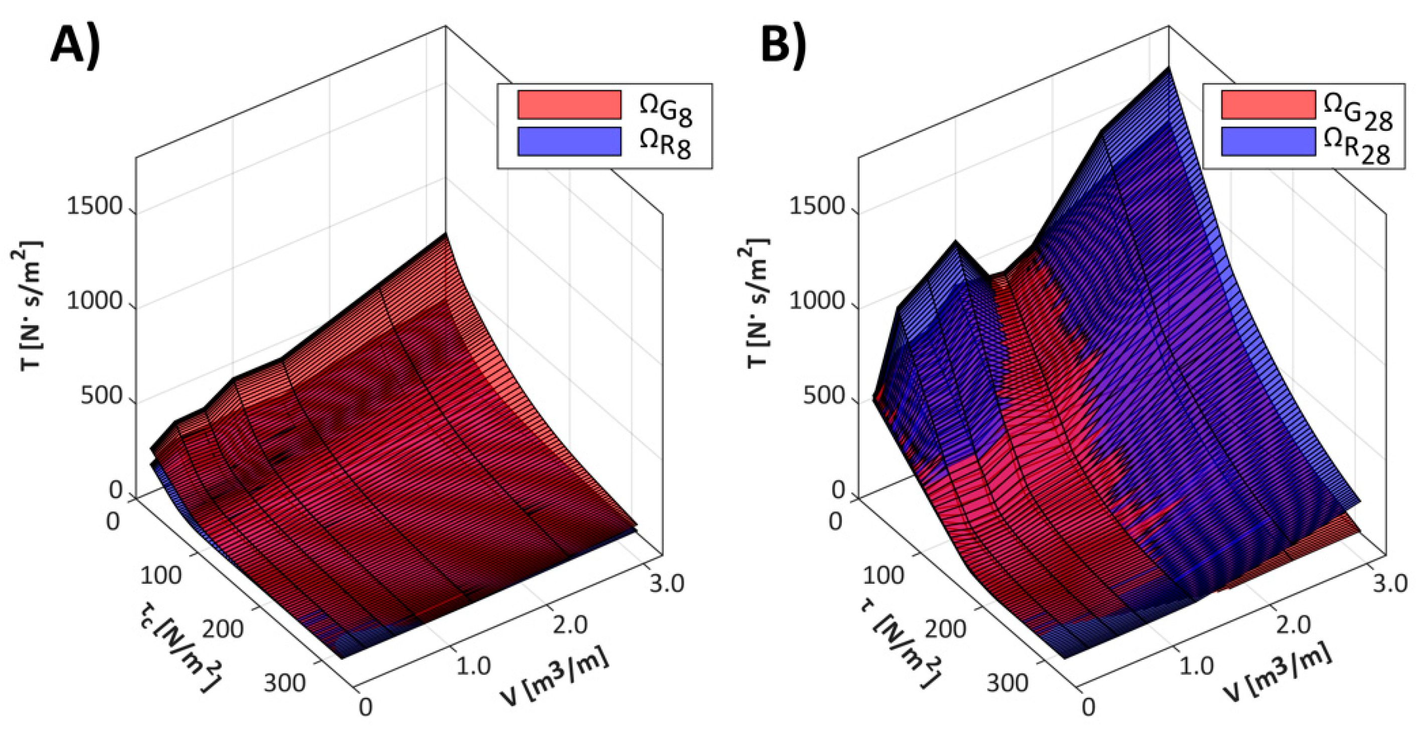
4.2. Emulator Surfaces Construction

Bed shear stress time series produced for each STP location from each CFD model and each wave volume (0.15, 0.4, 0.7, 1.0, 1.5, 2.5, 3.2, and 4.5 m³/m) are used to generate the training data of the emulators. To do that, each of these time series was integrated in time for one given value of ${\tau }_c$ in steps of 1 N/m² until 300 N/m². The ${\tau }_c$ range was defined based on the recommended values for grass and soil presented in Ref. [36]. As a result, lists of training data sets of three columns ($V$,${\tau }_c$, and ${\rm T}$) for each STP location were obtained and used to train the emulators.

A data-based emulation approach was selected [27], as we are only interested in the final ${\rm T}$ values for estimating the erosion depth in each location. A data-based emulator reproduces input-output relations from the input-output datasets produced by the CFD models. A 3D linear interpolation surface was used to build the emulators [47]. Each emulator on each location is defined as ${\mathsf{\Omega }}_{R_n}$ and ${\mathsf{\Omega }}_{G_n}$ according to the referred dike model. The Greek letter $\mathsf{\Omega }$ denotes emulator, letters R or G denote either “RCD” or “GCD” and the sub index $n$ denotes the STP location. These emulators were built based on the Matlab^® (MathWorks Inc., Natick, MA, U.S.) interpolation scientific package and were designed as 3D surfaces for estimating the ${{\rm T}}_{G_n}$($V$,${\tau }_c$) and ${{\rm T}}_{R_n}$($V$,${\tau }_c$) functions in each STP. The emulators on STP8 and STP28 (${\mathsf{\Omega }}_{R_8}$, ${\mathsf{\Omega }}_{G_8}$, ${\mathsf{\Omega }}_{R_{28}}$, ${\mathsf{\Omega }}_{G_{28}}$) are plotted as an example in Figure 6 to show what the surfaces look like. In total, 66 emulators were built to predict ${\rm T}$ as a function of $V$,${\tau }_c$; 33 for the RCD and 33 for the GCD. These emulators can calculate the set of ${\rm T}$ values of 1000 storms in less than 10 s on a standard personal computer. Note that the surface that corresponds to the emulator of a dike with a road on top (${\mathsf{\Omega }}_{R_{28}}$) presents a less smooth behaviour along the slope with respect to the grass emulation surface in the same location (${\mathsf{\Omega }}_{G_{28}}$), which demonstrates that there is indeed a significant effect derived from the presence of the road upstream. This also shows that the overtopping bed shear stress process is non-linear and may be under- or over-estimated when irregularities are not explicitly considered.

For estimating the scour depth per wave, the emulators become very powerful as they are equivalent to the solution of the excess shear stress integrals present in the right side of Equation (4) (Figure 1), as presented in Equations (7) and (8) for both GCD and RCD cases, respectively.

$${\mathsf{\Omega }}_{G_n}\left(V,{\tau }_c\right)\approx \underset{t_i}{\overset{t_{i+1}}{\int }}\left({\tau }_{G_n}\left(V,t\right)-{\tau }_c\right)dt$$

(7)

$${\mathsf{\Omega }}_{R_n}\left(V,{\tau }_c\right)\approx \underset{t_i}{\overset{t_{i+1}}{\int }}\left({\tau }_{R_n}\left(V,t\right)-{\tau }_c\right)dt$$

(8)

These emulators are valid for estimating the ${\rm T}$ values of any given wave volume ($V$) value between 0.150 and 3.2 m³/m and for any given ${\tau }_c$ value between 1 and 300 N/m². The ${\tau }_c$ value reflects the grass quality and hence when erosion occurs. At the same time, the resistance is also affected by the coefficient of erodibility $C_E$ (see Equation (4)) which represents the resistance of the cover to be eroded which is referred in this manuscript as the grass quality.

4.3. $C_E$ Functions

The $C_E$ coefficient determines the resistance of the grass to be eroded as a function of the ${\tau }_c$ in the selected erosion model as shown in Equation (2) [19]. In the present methodology, it is assumed that $C_E$ is a function of ${\tau }_c$ instead of a constant value which ensures that the same grass quality is reflected in both the estimation of ${\rm T}$ and the erosion depth estimation so that Equation (2) still remains valid for any ${\tau }_c$. These $C_E$ functions were built using the pre-trained emulators, the WOS released volume list from the experiment Part I, and the q10_sc2 and q50_sc5 scanned profiles [39]. These two scans represent the initial and final state of the 0.05 m³/s/m storm condition experiment. The functions were calculated for each STP as:

$$C_{E_n}\left({\tau }_c\right)=\rho {’}_{cover}\frac{-{\int }_{x_i}^{x_{i+1}}d\epsilon }{{\mathsf{\Omega }}_{R_n}\left(V,{\tau }_c\right)}$$

(9)

This equation was obtained by substituting Equation (8) into Equation (4). This equation allowed us to generate $C_E$ curves for each SPT for an arbitrary ${\mathsf{\tau }}_c$ range between 1 and 300 N/m² in steps of 1 N/m². In each step, the actual release list of the volumes corresponding with the 0.050 m³/s/m storm condition was used as input for the RCD emulators to obtain a cumulative value of ${\rm T}$ for evaluating Equation (9). The initial and final profiles of the 0.050 m³/s/m storm condition were chosen for building the $C_E$ functions, as for storm conditions with a lower $q_m$ no significant scouring was obtained during the experiment. The scour depths ($\epsilon$) per location due to the $q_m=$ 0.050 m³/s/m experiment were obtained in each STP by subtracting both profile scans (Figure 7 lower plot).

They are equivalent to the solution of the negative integral present in Equation (9) for each location. For STPs 18, 19, 27, 28, and 29 where accretion was observed, the results were discarded and replaced by the closest one where erosion was found as the erosion model assumes that all material is fully washed to the downstream part.

Different grass cover relative densities ($\rho {’}_{cover})$ per unit of width are required for each $C_E$ curve depending on whether the final profile is located in the grass layer or inside the deeper clayey soil layer. As no field data was collected regarding this parameter, density values for each type of cover (grass or soil), reported in Ref. [48] were used as reference. They correspond to a saturated sample extracted from a Danish dike which was composed of 0.17 m of soil and 0.03 m of grass with a total average density of 1870 kg/m³. For this study, we assumed a reference density per unit of width value of soil (${\rho }_{cove{r}_{soil}})$ of 2000 kg/m³. Based on these values, it is estimated that the saturated density of grass solely (${\rho }_{cove{r}_{grass}})$ is 1100 kg/m³. The resultant $C_E$ curves obtained by the use of Equation (9) are presented in the results Section 5.2. It is acknowledged by the authors that these values may differ from the actual ones of Millingen. However, they are of good order of magnitude and even result in very similar $C_E$ values with respect to the ones reported in Ref. [19].

4.4. Probabilistic Safety Assessment

In general, failure mechanisms can be expressed as a limit state equation:

$$Z=R-S$$

(10)

where the variable $S$ represents the load (solicitation) and $R$ represents the resistance of the structure. The $Z$ term represents the marginal resistance which defines the state of the system as safe when positive and in failure when equal to zero or negative. Wave overtopping failure is a major threat to flood defence safety, because when the grass cover is completely lost, a rapid scouring process of the soil core may initiate a dike breach. Hence for the present study, failure is defined as the complete loss of the available grass cover in any location (STP). The grass cover layer thickness ($\delta$) is defined as the top 10 cm (Figure 5), based on Ref. [32,38].

The dike grass cover limit state function is obtained by rearranging Equation (4) and making it equal to the marginal strength term for each overtopped wave and then summing over all overtopping waves (Equation (11)). Here, $\delta$ represents the resistance term ($R$) and the second term describes the erosion that represents the solicitation ($S$).

$$Z=\mathsf{\delta }-{\sum }_{i=0}^{N_{\mathrm{ow}}}\frac{C_E\left({\tau }_c\right)}{\rho {’}_{cover}}{\int }_{t_i}^{t_{i+1}}\left(\tau \left(V,t\right)-{\tau }_c\right)dt$$

(11)

The failure state is reached if the grass cover is completely removed ($Z\le 0$). The emulators were used to compute the excess shear stress per overtopping wave. All overtopping waves during a storm condition together yield the accumulated scour depth, which is evaluated for every STP along the dike profiles for the cases with ($Z_R$) and without ($Z_G$) a road on top. The $\delta$ values in each location and their corresponding emulators were replaced in Equation (11) such that the limit state equation of the grass cover for both cases with and without a road in each location could be evaluated. The resultant limit state equations per STP are defined as the accumulated scour depth per storm condition ($Z_R$ and $Z_G$) as shown in Equations (12) and (13):

$$Z_R={\delta }_{R_n}-\sum _{i=0}^{N_{\mathrm{ow}}}\frac{C_E\left({\tau }_c\right)}{\rho {’}_{cover}}{\mathsf{\Omega }\mathrm{G}}_n\left(V,{\tau }_c\right)$$

(12)

$$Z_G={\delta }_{G_n}-\sum _{i=0}^{N_{\mathrm{ow}}}\frac{C_E\left({\tau }_c\right)}{\rho {’}_{cover}}{\mathsf{\Omega }\mathrm{R}}_n\left(V,{\tau }_c\right)$$

(13)

The available grass cover per location (${\delta }_{R_n}$ and ${\delta }_{G_n}$) is defined as a deterministic variable and was calculated as the difference in elevation between the surface profile and the soil core line (dashed lower lines in Figure 5). The cover relative densities of grass (${{\rho }^{\prime }}_{cover}$) were assumed to be constant all along the dike profile.

For every storm condition, possible storm realizations that consist of $N_{\mathrm{wo}}$ sets of values of $V$, ${\tau }_c$ were randomly sampled via crude Monte Carlo. These values are used to evaluate Equations (12) and (13) which result in one single value of $Z_R$ and $Z_G$ per realization for each STP. Statistical distributions of $Z_R$ and $Z_G$ per location were built from 1000 realizations of overtopping waves. For each tested storm condition (see

Table 3. Characteristic values of dike configurations and 7 tested storm boundary conditions for riverine dikes for the tested range of overtopping discharges.

	$\mathbf{Mean}\mathbf{Overtopping}\mathbf{Discharge}{\mathit{q}}_{\mathit{m}}$ [m3/s/m]
	0.0001	0.001	0.010	0.020	0.050	0.075	0.100
$D$ [h]	6	6	6	6	6	6	6
$R_c$ [m]	2.99	2.20	1.40	1.17	0.85	0.71	0.61
Slope [-]	1:3	1:3	1:3	1:3	1:3	1:3	1:3
$N_w$ [-]	6545	6545	6545	6545	6545	6545	6545
$N_{ow}$ [-]	65	458	2291	3142	4451	4974	5367
${\%}_{ov}$ [-]	0.01	0.07	0.35	0.48	0.68	0.76	0.82
$V_{max}$1 [m3/m]	0.21	0.46	0.94	1.27	1.91	2.35	2.72

¹ Maximum expected volume from Weibull distribution [12].

, $q_m$), the random sampling was done following a pre-fitted Weibull distribution. The failure probabilities per storm condition are then calculated from the distributions as $P_{f_R}$ ($Z_R\le 0$) and $P_{f_G}$ ($Z_G\le 0$) in each location. For each realization, a final eroded profile was also estimated by subtracting the accumulated scour depth (second term of Equations (12) and (13)) from the initial elevation profile (green lines of Figure 5). Note that each estimated value is conditioned to the event of the simultaneous occurrence of the boundary conditions of wind speed and water level. For the present study, the same boundary conditions were used for each storm condition but the crest level was modified so that different $q_m$ values could be obtained.

Individual wave volumes, $V$, were sampled from the two parameter ($a$ and $b$) Weibull distribution [49]. For the present study, it is intended to represent storm/wind surge overtopping events of duration D [h] composed of individual single wind generated waves $V_i$ that result in an overtopped volume distribution [50]. The cumulative exceedance function of this distribution is expressed as:

$$P_V=P\left(V_i\le V\right)=1-exp\left[-{\left(\frac{V}{a}\right)}^b\right]$$

(14)

For the scale ($a$) and shape ($b$), the method presented in [50] improved the estimation of $b$ for wave overtopping by fitting an empirical equation to experimental results (Equation (16)).

$$a=\left(\frac{1}{\mathsf{\Gamma }\left(1+\frac{1}{b}\right)}\right)·\left(\frac{q_m{T}_m}{{\%}_{ov}}\right)$$

(15)

$$b={\left[exp\left(-0.6\frac{R_c}{H_{m0}}\right)\right]}^{1.8}+0.64$$

(16)

where $q_m$ represents the average overtopping discharge [m³/s/m] of the storm, ${\%}_{ov}$ represents the overtopping percentage [-], $R_c$ represents the dike free crest height [m], $T_m$ represents the mean wave period [s], and $H_{m0}$ represents the incident energy based significant wave height [m]. Former Dutch guidelines [11] define the allowable q_m between 0.0001 and 0.01 m³/s/m depending on the type of cover, the outer slope revetment and the importance of the structure in the system [11]. This range plus four larger storm conditions were tested (Table 3).

All the storm conditions tested in this study (Table 3) corresponded to a wave ($H_s$ = 1 m and $T_p$ = 4 s), wind speed, and water level event with exceedance probability $P(H_s,T_p,q_m$) = 1 × 10⁻⁴, which is the design event (in the former legislation) for this particular dike location. All estimated failure probabilities obtained from the emulators are conditioned to this event ($P_{f_R}\left(Z_R\le 0|H_s,T_p,q_m\right)$ and ($P_{f_G}(Z_G\le 0|H_s,T_p,q_m)$). For calculating the failure probability per location on each model we rely on the use of the conditional probability so that $P_f\left(Z\le 0\cap H_s,T_p,q_m\right)=P_f\left(Z\le 0|H_s,T_p,q_m\right)\times P(H_s,T_p,q_m$).

For the ${\tau }_c$ random variable, there is no available literature to our knowledge that studied or suggested the stochastic nature (distribution or moments) of this variable for grass. However, from the values reported in Ref. [39], an equivalence curve between critical erosion velocities $U_c$ and ${\tau }_c$ was built based on the table presented in Ref. [36], as shown in Figure 8. This equivalence curve allowed the transformation to define the $C_E$ as a stochastic random variable.

The stochastic distributions for the $U_c$ of grass and soil, were taken from Ref. [21]. This work concluded that $U_c$ can be represented by a log-normal distribution for the grass cover and by a generalized extreme value (GEV) distribution for bare soil locations. The parameters for the GEV distribution could not be estimated from the experimental data collected during the Millingen experiment. Hence, a log-normal distribution was also assumed for the bare soil spots, as presented in

Table 4. Stochastic random variables of cover quality $U_c$ used as input for C_E calculation. CoV is the coefficient of variation and QCF is grass quality correction factor for poor, average, and good.

		$\mathbf{Clay}{\mathit{U}}_{\mathit{c}}$	$\mathbf{Grass}{\mathit{U}}_{\mathit{c}}$
		Good	Poor	Average	Good
Distribution	[-]	Log-norm	Log-norm	Log-norm	Log-norm
mean	[m/s]	0.85	3	4	6.5
CoV	[-]	0.1	0.3	0.3	0.3
QCF	[-]	-	1.5	1	0.1

.

Based on the indicative average values of ${\tau }_c$ presented by Ref. [36], it was possible to define mean values of $U_c$ per grass and soil qualities. The coefficients of variation (CoV) were calculated from the $U_c$ statistical distributions presented by Trung [21]. The grass quality correction factor (QCF) is obtained by estimating the value which shifts the “average” $C_E$ grass quality function towards the recommended values in Ref. [19].

5. Results

5.1. CFD Calibration and Validation

Calibration and validation of the RCD model were carried out as in Ref. [26], using the observations of the Millingen experiment part II. In Ref. [26], it is concluded that although the depth simulations show some deviations, the simulated velocities along the crest and slope are within 20% of the observations. A detailed analysis of the effects and estimated errors derived from the mesh refinement, the CFD RANS parametrization, and the temporal effects in the shear stress time series error can be found in Ref. [26]. The flow depths and velocities for the GCD case are in good agreement with the ones fitted for the Vechtdijk experiment (Appendix A and Appendix B). Also, in this case, the simulated velocities are more accurate than the depth simulations. In the modelling approach, erosion is computed based on excess shear stress. Appendix C shows that for most wave volumes, both the GCD and RCD models simulate the duration of the overtopping waves quite well. Especially, the magnitude and timing of the velocity and depth at the wave fronts are simulated well.

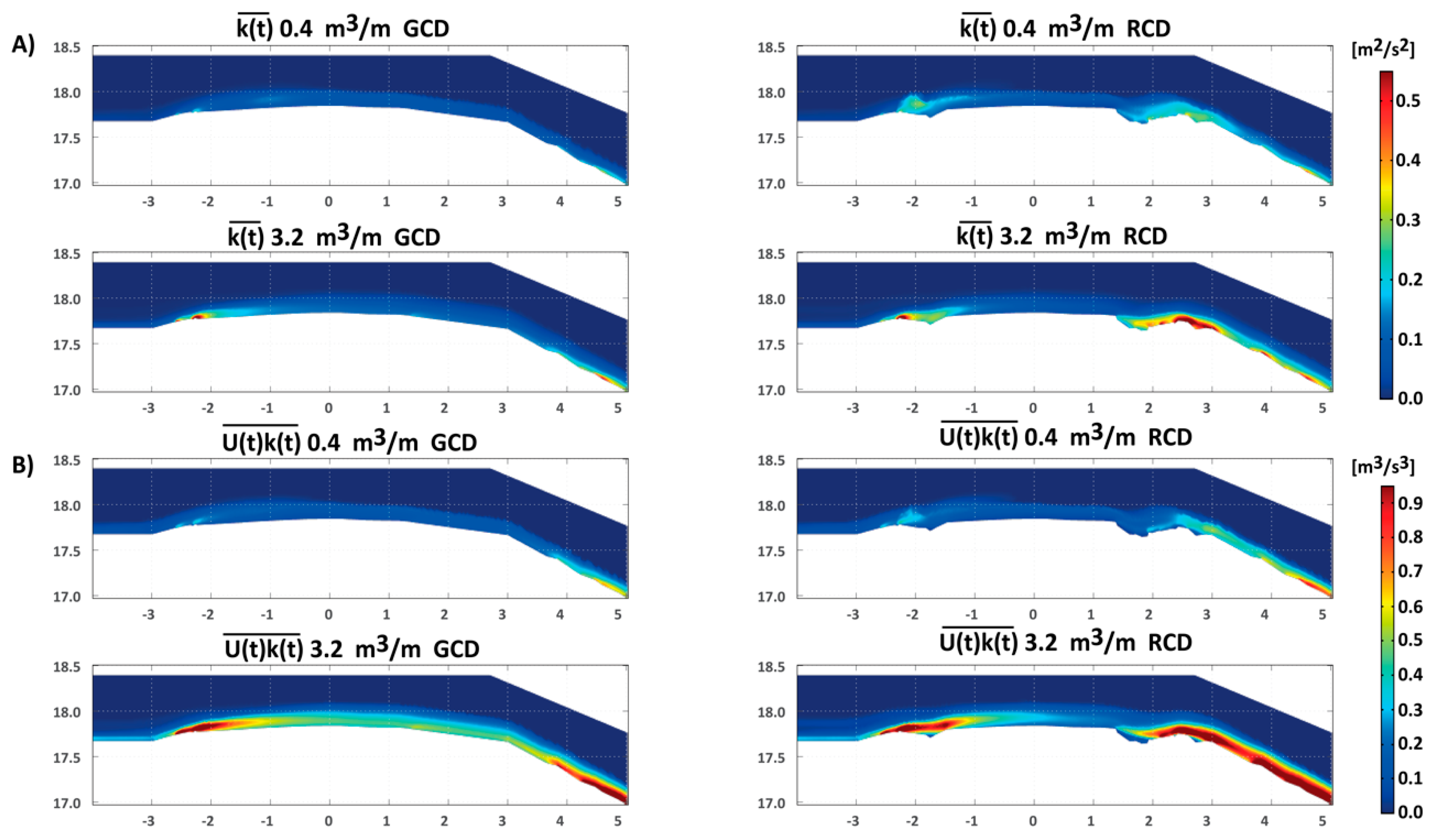
5.2. Effects of Turbulence on the Excess Shear Stress $\overline{T}$

Both the RCD and GCD model results show highly turbulent flow over the dike profile with Reynolds values between 10,000 and 200,000 for the 0.15 and 3.2 m³/m volumes, respectively, with supercritical flow (Froude between 10 and 2 for 0.15 and 3.2 m³/m volumes, respectively). Low Froude numbers are observed for the RCD model in STP 14 Fr ≈ 1 at the adverse bottom slope. For abrupt changes in the bottom geometry, the use of a single depth-averaged turbulence factor along the entire profile may either underestimate or overestimate the locally exerted bottom shear stress as the turbulence intensity changes significantly along the dike profile. This can be observed in Figure 9A, where the average kinematic energy in time ($\overline{k\left(t\right)}$) for waves of 0.4 m³/m and 3.2 m³/m in both GCD and RCD models is shown. These plots show that the highest values of turbulence occur at the locations where abrupt bottom changes (irregularities) are observed.

Nonetheless, the amount of erosion does not solely depend on the amount of turbulence but also on the momentum of the fluid. This implies that high erosion potential may also occur at low turbulence locations due to the acceleration of the flow. Hence, the average of the product between mean velocity ($U\left(t\right)$) and kinematic energy ($k\left(t\right)$) averaged in time allows one to determine the highest potential erosion locations, as shown in Figure 9B. Note that these plots do not directly imply which locations are more prone to erosion as the cover resistance is also a determining factor.

The bottom shear stress $\tau \left(t\right)$ intrinsically contains the effects of turbulence. Hence, they are influencing the probabilistic estimation as they also influence $T$. To observe this effect, the release volume list used as input for the 0.050 m³/s/m test is used to calculate a $T$ value per volume while assuming ${\tau }_c=0$. From the produced set of $T$ values, the average shear stress excess ($\overline{T}$) value and 95% confidence bounds per location for each of the 33 locations in both cases were calculated and plotted in Figure 10.

The ratio between the $\overline{T}$ values of the RCD and GCD cases (Figure 10, bottom) shows that $\overline{T}$ is around 2 to 4 times larger in the road transition zones, which correspond to the high turbulent kinetic energy regions on Figure 9. Additionally, the $\overline{T}$ values in the upper part of the landward slope (between STPs 26 and 33) were larger in the RCD with respect to the GCD. This behavior was surprising as the landward transition gap was expected to dissipate energy. However, the turbulence generated in the transition propagates downstream (see $\overline{U\left(t\right)k\left(t\right)}$ in Figure 9) and probably induces an increase in the potential erosion of the landward upper slope.

From these results, it is also possible to identify the effects of surface roughness and bottom surface irregularities separately. On one hand, due to form roughness, the $\overline{T}$ values increase significantly after STP 9 where evident abrupt bottom changes are present in the RCD case. On the other hand, the$\overline{T}$ in the centerline location (STP8) of Figure 10 is lower in the RCD case, which can be attributed to the smoother surface. This can be corroborated from Figure 9 at the same location where the bottom slope is almost the same in both models. At this location, the turbulent kinetic energy is also very similar and yet the erosive potential is much greater in the crest for the GCD.

Except for STP8, all locations present equal or larger $\overline{T}$ values in the RCD with respect to the GCD. From a probabilistic point of view this means that on average, the probability of scouring at these locations will be higher if grass quality and cover thickness remain constant along both profiles.

Interestingly, the 95% confidence bounds show a wider spreading with respect to the mean values in all locations with high erosive potential. This is concluded by correlating the spreading of the confidence bounds per location of Figure 10 with respect to the locations of highest values of $\overline{U\left(t\right)k\left(t\right)}$ in Figure 9B. Similarly, it can be observed that at locations where bottom slope changes are minimal (e.g., STP8), less spreading of the confidence bounds is observed which indicates that there is less turbulence.

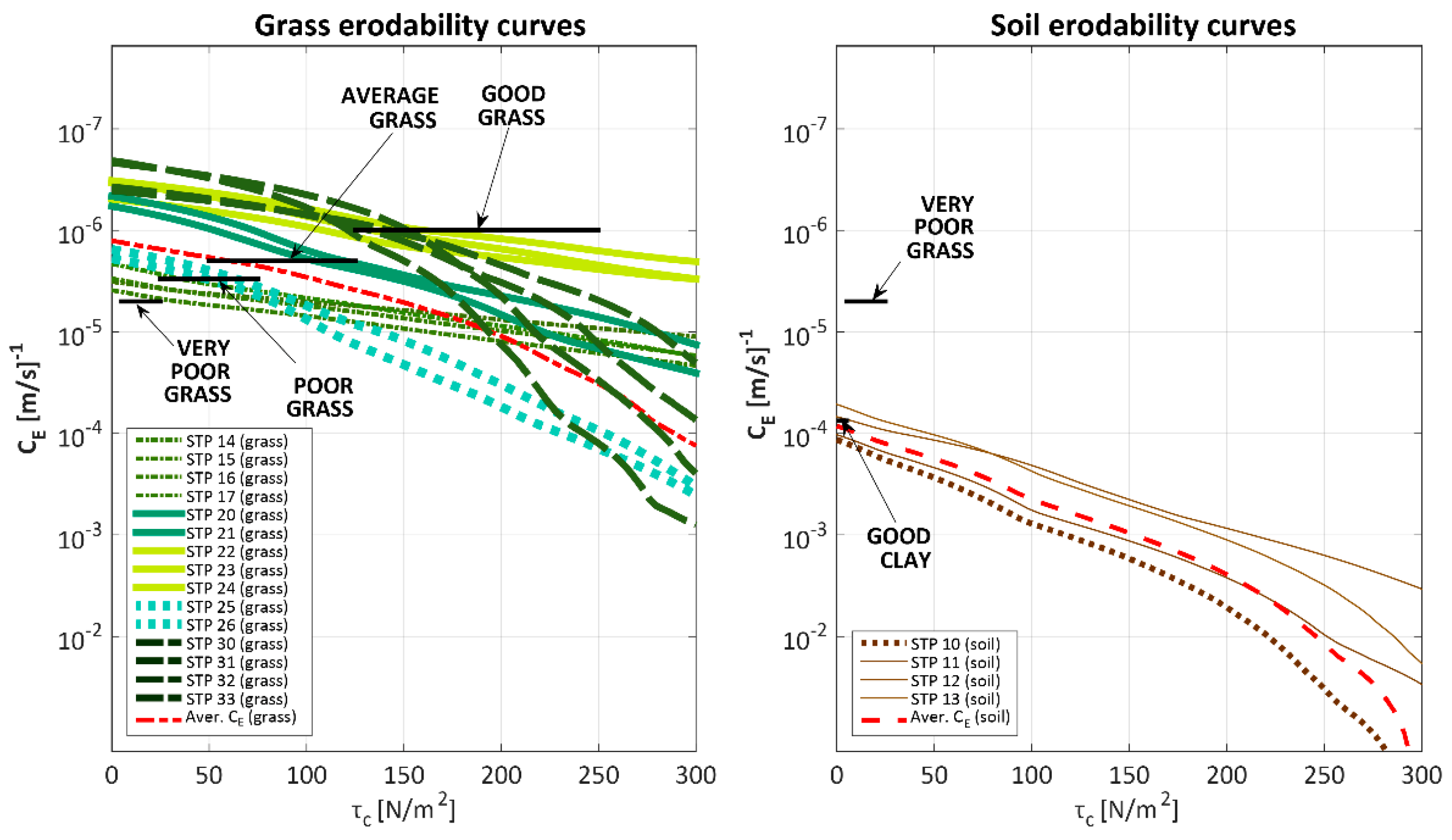
5.3. CE Curves Calculated from Millingen Measurements

The $C_E$ curves obtained from the experiment data are presented in Figure 11. The results are presented in Figure 5 and correspond to an estimation of the corresponding curve of grass quality of each of the places where erosion was found along the dike cross sectional profile during the Millingen experiment. This figure only includes the resulting CE curves for STPs located after the asphalt cover (STPs > 9), which were influenced by the presence of the road. The right plot of Figure 11 shows the CE curves obtained for SPTs inside the gap where no grass cover was present and consequently correspond to soil erodability values.

The $C_E$ curves from the STPs located closer to the road (STPs 14 to 17 plotted as dense dashed lines in Figure 11) cross the grass quality reference intervals suggested by [19]. Thus, we classified them between the very poor and poor grass quality. For STPs located over the vertex plotted as continuous thicker lines (STPs 20 and 26) coincide with average and good grass quality reference intervals. For STPs 25 and 26 which are located in the dent after the vertex, poor grass quality $C_E$ curves were found. The presence of such a dent may be a good indication of deterioration due to traffic which explains such low quality just after spots of good quality. The rest of the profile (mostly along the inner slope in STPs 30 to 33) present good grass quality. These results are in good agreement with the field findings for grass quality reported by [39]. For the STPs located initially in the soil zone, good clay quality values were obtained (right plot of Figure 11). For the GCD case, no information about grass quality was available. Therefore, we used the average $C_E$ curve, corresponding to average grass quality. It is acknowledged that a dike without a road may have better quality in reality than what we assumed as we used the transition zone data in the averaging procedure for obtaining the $C_E$ “average curve”.

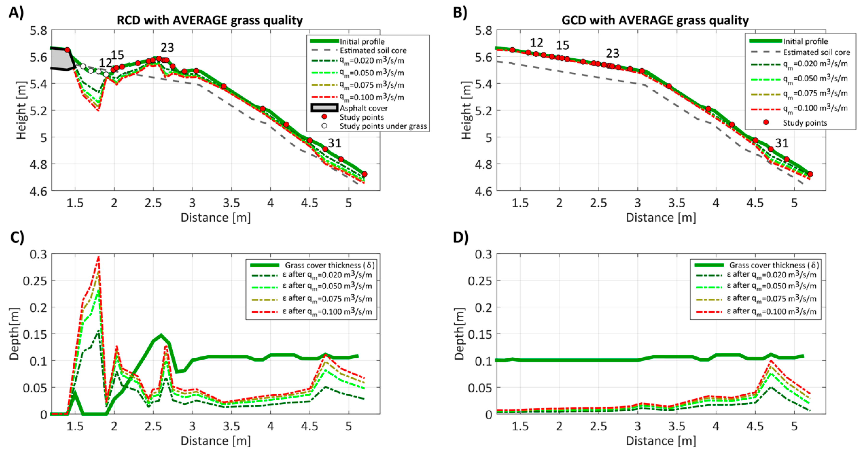
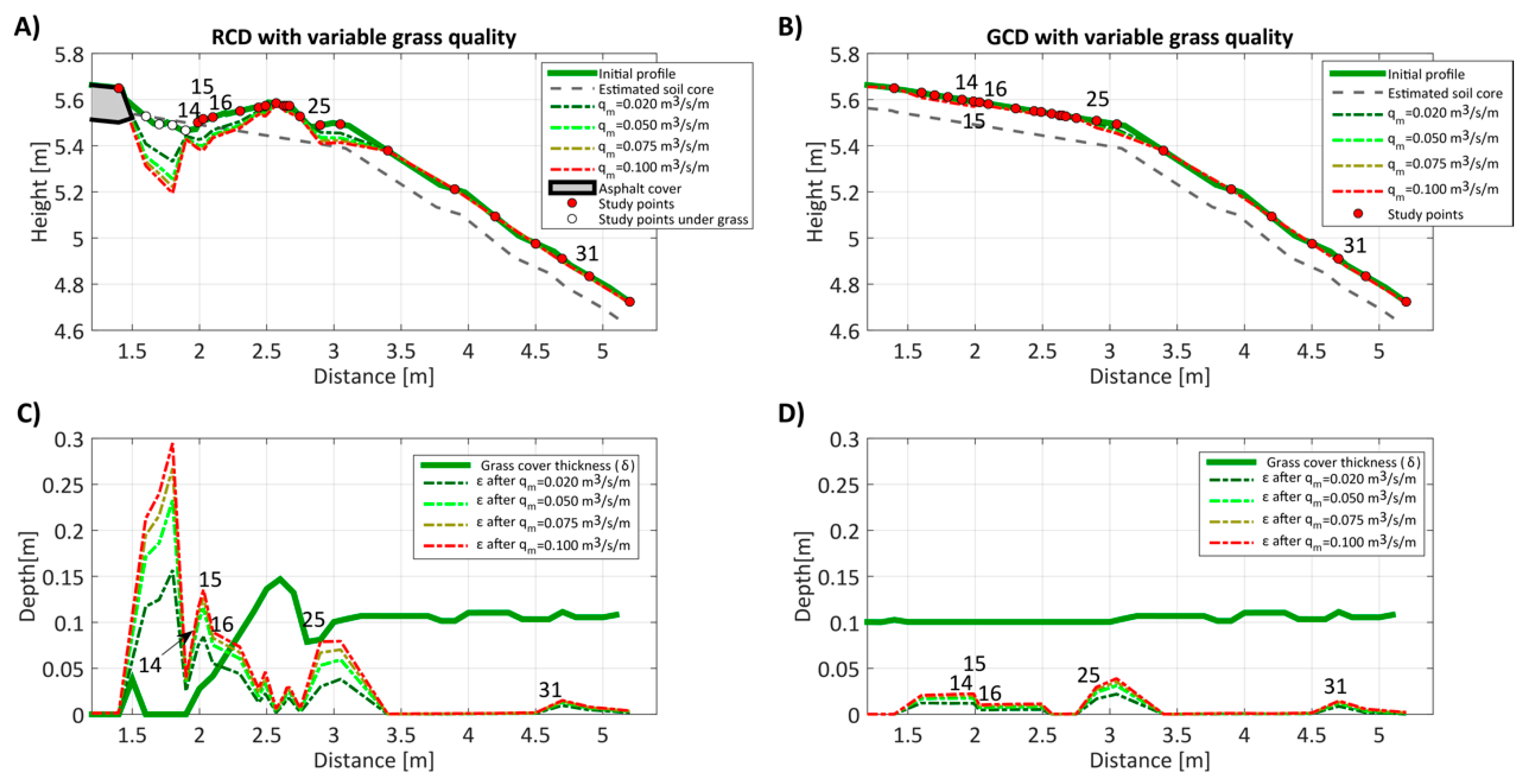
5.4. Scour Depth Profiles

The results of the simulations for the storm conditions of $q_m$ 0.0001, 0.001, and 0.010 m³/s/m showed almost no scouring with the 1000 samples. Therefore, only the scour profiles for the largest $q_m$ (0.02–0.1 m³/s/m) were analyzed. Each profile was produced by plotting the mean value of the final scour depths for each STP after the 1000 realizations generated for each $q_m$ (Table 3). These values are equivalent to the mean value of the probability density function obtained for the second term of Equations (12) and (13) for the 1000 sampled realizations in each STP. The profiles were only analyzed for the STP locations after the asphalt cover.

For the first part of the analysis, the simulations were done assuming a uniform average grass quality along the whole profile. The obtained scoured profiles (see Figure 12) show that the large failure spot in the lower part of the RCD may be explained from the additional energy available due to the presence of a smoother upstream surface (asphalt cover) and the momentum gain when flowing downslope. Moreover, an eventual increase of the turbulent flow due to the slope bottom irregularity around x = 3.8 m near STP 28 may also contribute. Another significant scour zone is observed on the transition between bare soil (STP12) and the dike crest vertex (STP23). These deep erosion spots coincide with the locations where the initial profile has an adverse slope. These zones are identified as the initiators of turbulence in the flow as it can be observed in Figure 9.

From these results, the most interesting finding is that STP23 represents a weak spot in the profile despite the fact that the available grass cover is even thicker than most of the other locations. This can be explained based on Figure 9 and Figure 10, where STP23 corresponds to one of the most turbulent locations. Again, this supports the importance of including a highly detailed geometry and its derived turbulence effects in modelling of dike cover erosion.

For a more realistic representation of the grass cover erosion, the grass qualities of each point were replaced by one of the three estimated qualities presented in Table 4, that seemed closer to the local condition per STP found in Section 5.2. The resultant scoured profiles (Figure 13) become safer in the lower part of the slope (STP 31) for both RCD and GCD as better grass quality than average was obtained in that zone.

However, two new close to failure locations were identified in STPs 25 and 26 which were not observed when assuming all grass quality as average. For the 0.1 m³/s/m RCD storm profile, it can be observed how STP 25 is very close to failure as the scoured depth is very close to the available grass cover thickness (lower left plot in Figure 13). This location corresponds to the most prone to fail spot in the GCD given the poor grass quality present in that particular location.

5.5. Probability of Failure

The failure probabilities for both dike cases are presented in Figure 14. For this study, any failure probability larger than 9.9 × 10⁻⁵ is assumed as an already failed spot. This value was assumed since STPs 10, 11, 12, and 13 (located in bare soil) presented values above this threshold and were already in failure state (no grass cover) before routing each different storm condition and where not taken into account for the dike assessment.

For the present study, it is assumed that the failure probability of the configuration to be studied is equal to the largest value found along the profile. This allows us not only to define the failure probability but also the spatial location of the failure which can later be related to the analysis of the origin of the failure.

Figure 14 shows that the dike without a road presents significant failure probabilities in the slope on STP31 with Pfs of 5 × 10⁻⁵ and 8.2 × 10⁻⁵ for the $q_m$ 0.075 and 0.1 m³/s/m. The results for this last configuration show that the probabilities of failure along the landward slope are almost identical for both RCD and GCD cases for the largest tested $q_m$. This means that when using the failure criteria of assigning the maximum failure probability along the profile for a single storm it could be concluded that both dikes with and without road have almost the same failure probability. Yet, for lower $q_m$ (<0.075 m³/s/m), the probabilities of failure of the landward slope are always higher in the dike with a road. It is also observed on STP25, that a sudden potential failure spot is created for a $q_m$ larger than 0.050 m³/s/m. It is described as sudden because the failure probability was less than 1 ×10⁻⁴ for lower storms with poor grass quality. This can be explained due to the highly turbulent flows expected in this location (see Figure 9).

Also, the assessment was performed with the spatially varying grass quality based on observed grass quality in the Millingen experiment to represent a more realistic estimation. Here, a sudden failure spot is observed in STP25 for a 0.1 m³/s/m storm (see Figure 15).

These results show that for the dike with a road, the maximum probability of failure is equal to 5 × 10⁻⁵ for the largest storm in STP25. Based on all previous analyses, STP25 presented a high $\overline{T}$ value combined with poor grass quality and medium to high grass cover thickness ($\delta =7.8$ cms). This means that for this particular place, turbulence plays a more important role than cover thickness as STP25 represents the highest failure potential spot on the dike while also presenting the highest value of average kinetic energy (see Figure 9). From this last figure, it is expected that this dike will present its first failures occurring nearby the already scoured zones (STP14 to STP18) with Pf range between (1 × 10⁻⁵ and 1 × 10⁻⁴) for the case where the road is present. For the no road configuration, it is expected to have a Pf lower than 1 × 10⁻⁶.

6. Discussion

6.1. Uncertainties in the Modelling Process

In this paper, a methodology is presented to predict the spatially varying probability of failure along the grass cover using emulation of a highly detailed CFD model. The P_f values obtained for each location are conditional to the upstream and the downstream locations. This means that the turbulence effects are captured in the emulators as they are trained based on the time series from the CFD model which includes them by solving for the kinematic energy variable in time and space. One of the main assumptions in this study is that the CFD models can be validated by checking the order of magnitude and trends of water depths and maximum velocities in two points along the profile (See Appendix A, Appendix B, and Appendix C). However, the main output of the CFD models used in this study is the produced bed shear stress which cannot be validated at this stage, because no data was collected regarding this quantity during the experiments. Yet, we are confident that the model is giving consistent results in terms of order of magnitude. The uncertainties of the CFD model and assumptions in the erosion model determine the accuracy of the emulators and therefore the probabilities. Therefore, in order to increase the accuracy of the final failure probabilities, the first step is to improve and better validate the CFD models. In general, the presented methodology can be applied to other CFD models as well.

Additionally, the scouring process is highly time-dependent as the dike profile changes in time (not only due to erosion, but also due to accretion). Consequently, hydrodynamics change in time as well. In that sense, the emulators built for this study become more uncertain for larger storms as the chances of significant change in the dike profile become larger. This means that the updating of the bottom profile should be done after each routed wave and not after the complete storm. However, for the present methodology, the resultant profiles are a function of the emulators, which use a set of 1000 realizations for each storm, generated independently from the set of volumes used in the Millingen experiment and yet they result in very similar scour patterns compared to the one observed during the Millingen experiment. This indicates that even though the CFD model and its emulators were not perfect, and the profiles were not updated after each wave overtopping, the bed shear stress stochastic nature is fairly well represented by the emulators, plus it allows one to make scenario assessments without rerunning the original models.

Regarding the erosion model adopted for this study, it is also acknowledged that it fully attributes the complete erosion process to the bottom shear stress, whereas, in reality, normal stresses also contribute. This choice was made to actually reduce the uncertainty as using more complex erosion models requires a larger amount of data with their associated uncertainties potentially making the model even more uncertain. Still, the results obtained for the erodibility functions ($C_E$) also show good agreement with the suggested reference values deducted from field measurements and literature. This may be a good indicator that the simpler adopted erosion model is sufficiently robust for probabilistic modelling.

6.2. Sensitivity to the Grass Quality Estimation

Grass quality is highly variable in space and difficult to determine [36] in field experiments. Therefore, we inferred the grass quality for the test location from the observed erosion depths and emulators and we subsequently compared different configurations of grass quality. The inferred grass quality was better along the slope than on the crest where thickness was smaller, but the results showed that grass quality is not necessarily correlated to the available grass cover thickness which is another factor that determines the resistance to erosion. An example of this can be found for STP21 and STP26 where $\epsilon$ is larger than 0.10 m for both locations and still the estimated grass qualities were good and poor. These examples show that grass quality also has a significant effect on the occurrence of reduced failure probabilities. For example, the failure probability in the RCD with more realistic grass quality distribution was 5 × 10⁻⁵ while presenting a poor local grass quality in STP 25. The failure probability in this same location for the same dike case is close to zero by just changing the grass quality to average (see Figure 14). This shows that the safety assessment cannot be done solely from the hydrodynamic point of view as the erosion pattern differs from the expected one using highest $\overline{T}$ values only. Poor grass quality spots have a high probability of failure despite the magnitude of $q_m$. Additionally, the RCD more realistic model also presents a failure probability of 6 × 10⁻⁵ in the landward vertex (STP 25, Figure 15) during the most severe storm, whereas the realistic GCD has almost a negligible probability of failure in this same location. The variability on the grass cover may be attributed to an external factor such as traffic which, for the case of a dike with a road on top, is inevitable.

Accurate observations of grass quality were therefore essential in our study case. However, we used a relatively simple approach to infer the grass quality from the erosion scanned profiles. For further applications of the methodology, detailed grass quality data is required, which can be derived from dike inspections or, possibly, remote sensing methods.

It is acknowledged that grass quality will also vary in the longitudinal direction. The present study assumes that the dominant direction of the generated shear stresses occurs in the cross-sectional direction (from crest to landside) and, therefore, the most probable way to determine failure is in that direction. However, with the constant modification of the cross section during the erosion process it can happen that grass quality and shear stresses importance vary their dominant direction. These effects cannot be considered with the present method and may be worth further studying.

6.3. Applications of the Probabilistic Method

The results show that the probability of failure if a road is present is higher along the simulated dike section, with respect to the case without a road, for all storms and grass qualities tested. However, for the GCD case with variable grass quality, all estimated failure probabilities (Figure 15) were less than 1 × 10⁻⁶. This result does not imply that the dike is 100% safe at these spots, because the small failure probabilities are predicted less accurately. The reason for the latter is that the 1000 samples of the Monte Carlo assessment were probably not sufficient to explore the tail of the distribution in depth as their associated P_f can be smaller than the ones obtained for a Monte Carlo standard error >3%. The methodology presented in this paper enables the use of such a high number of computations within a feasible time period. However, a more extensive probabilistic analysis, including the uncertainties in the modelling process and increasing the number of samples (lower standard error in the Monte Carlo) and using smart sampling techniques to cover the tail will greatly increase the accuracy of the predicted probability of failure.

The method can be extended by including the wave parameters and water levels during the random sampling by making them stochastic variables fitted to data series of storm wave conditions and water levels [51]. This allows one to extend the method to a fully probabilistic analysis by including the wind speeds water levels uncertainties explicitly. The resulting overtopping volumes are used as input for the emulators presented in this study, allowing one to derive fully probabilistic failure values along the dike profiles. Nevertheless, it remains a challenge to fully analyze the implications of such an extensive analysis and this is recommended for further study.

One of the main assumptions in the methodology was the definition of failure of the dike cover if the erosion depth exceeded the grass cover thickness of 10 cm. This assumption is highly arbitrary and debatable. However, no definition of failure for wave overtopping is available, other than a dike breach, which is a highly complex process caused by many interacting failure mechanisms and therefore too difficult to model. The adopted 10 cm threshold has obviously large consequences for the resulting probabilities. In order to achieve realistic values for the failure probability due to wave overtopping, we recommend more research to achieve a more advanced definition of the threshold of failure.

To summarize, the precise quantification of the low failure probabilities is more uncertain, but it is expected that they will still be in the obtained order of magnitude, which is sufficient to draw a good conclusion from the study in terms of trends and locations. The spatially distributed failure probabilities become useful, not only to determine the most prone to failure location, but also to stress their analysis during the yearly visual inspections for Dutch dikes. The quantification of the local probabilities of failure is input for any probabilistic dike safety assessment or probabilistic design. These results become even more relevant in cases of dike concepts such as the unbreachable dike and the multi-functional flood defence [51] which are designed to cope with climate change [5] and to withstand large amounts of overflow and storms similar or larger than the largest ones tested in this study.

7. Conclusions and Recommendations

This study shows a methodology to assess the spatially distributed probability of failure of a dike, with and without a road on the crest, due to wave overtopping erosion. In our case, the presence of a road on the dike increased the erosion of the grass cover and increased the probability of failure locally and for the entire dike profile. Probabilities were derived using a novel emulation method. Based on the obtained results of the study, specific conclusions for the two cases can be summarized as:

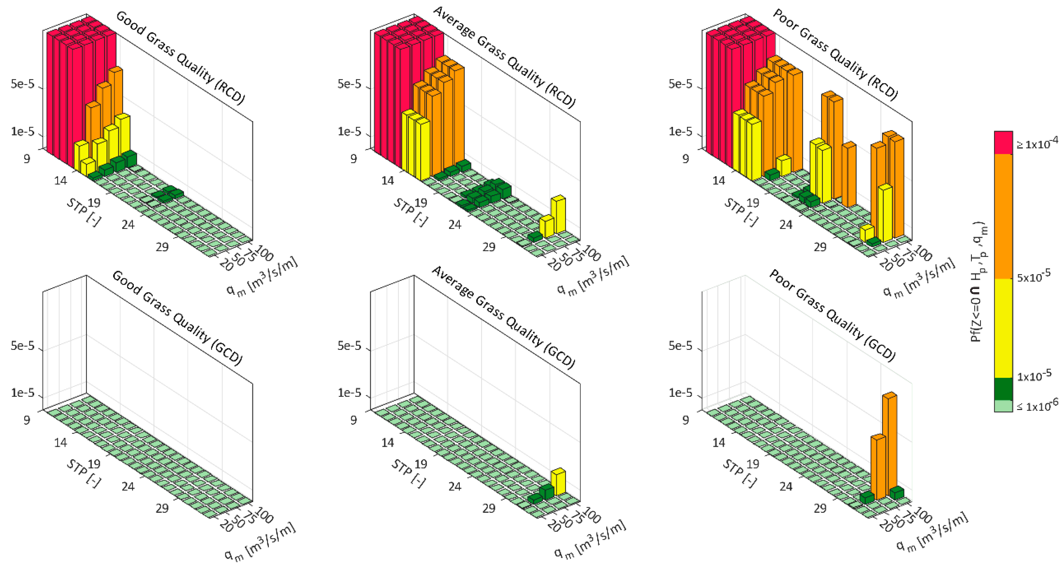
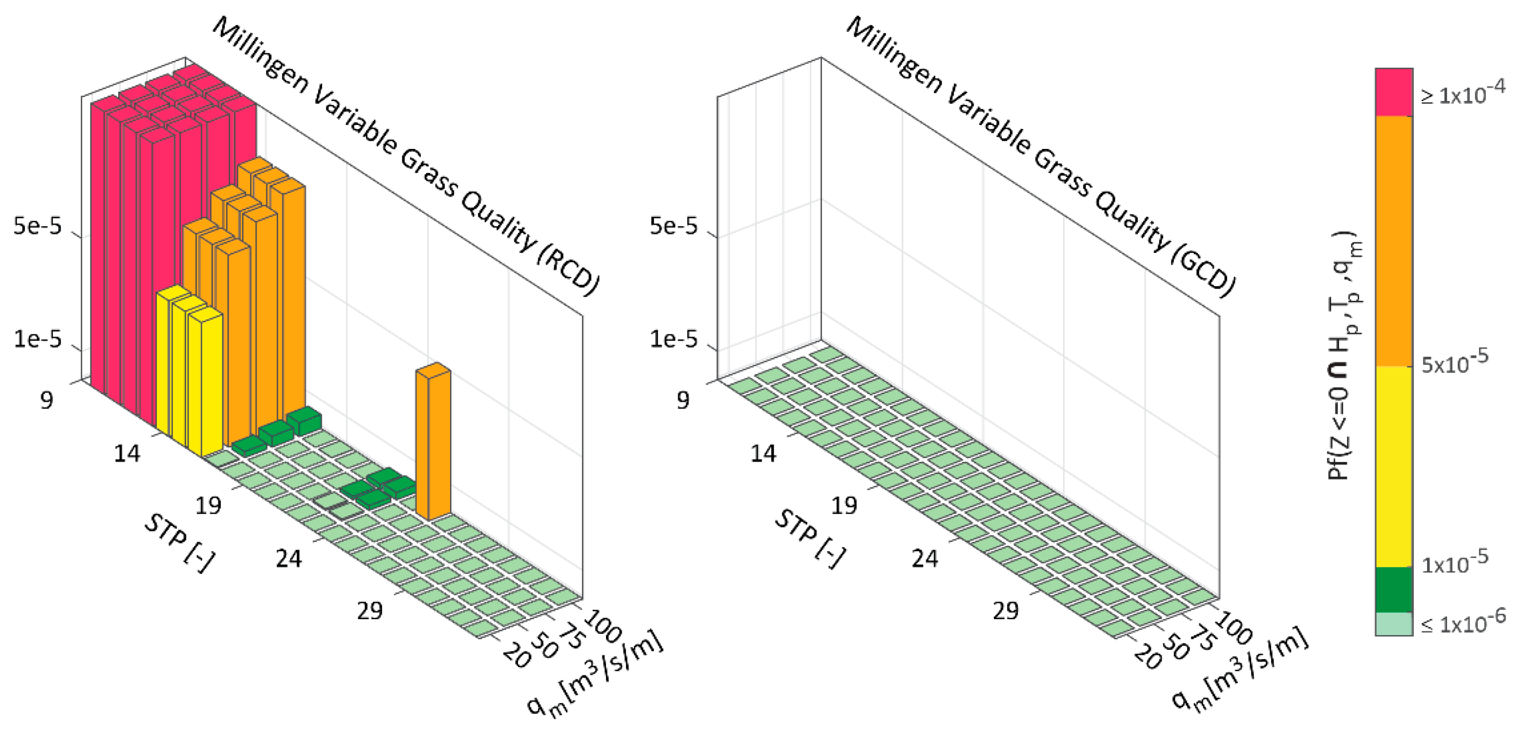
• The dike with a road showed higher probabilities (5 × 10⁻⁵ > P_f > 1 × 10⁻⁴) of failure with respect to a dike without a road (P_f <1 × 10⁻⁶) if realistic grass quality distribution was assumed. The probability of failure in the zones where higher initial deterioration was observed (e.g., locations immediately next to the road and over the vertex) is significantly higher with respect to the remaining part of the dike. Yet, these locations also correspond to spots where higher turbulence was observed with respect to the remaining part of the locations along the dike profile. However, if good quality grass was present all along the dike, both dike cases will present very low failure probabilities along the slope and the vertex (P_f < 5 × 10⁻⁵).
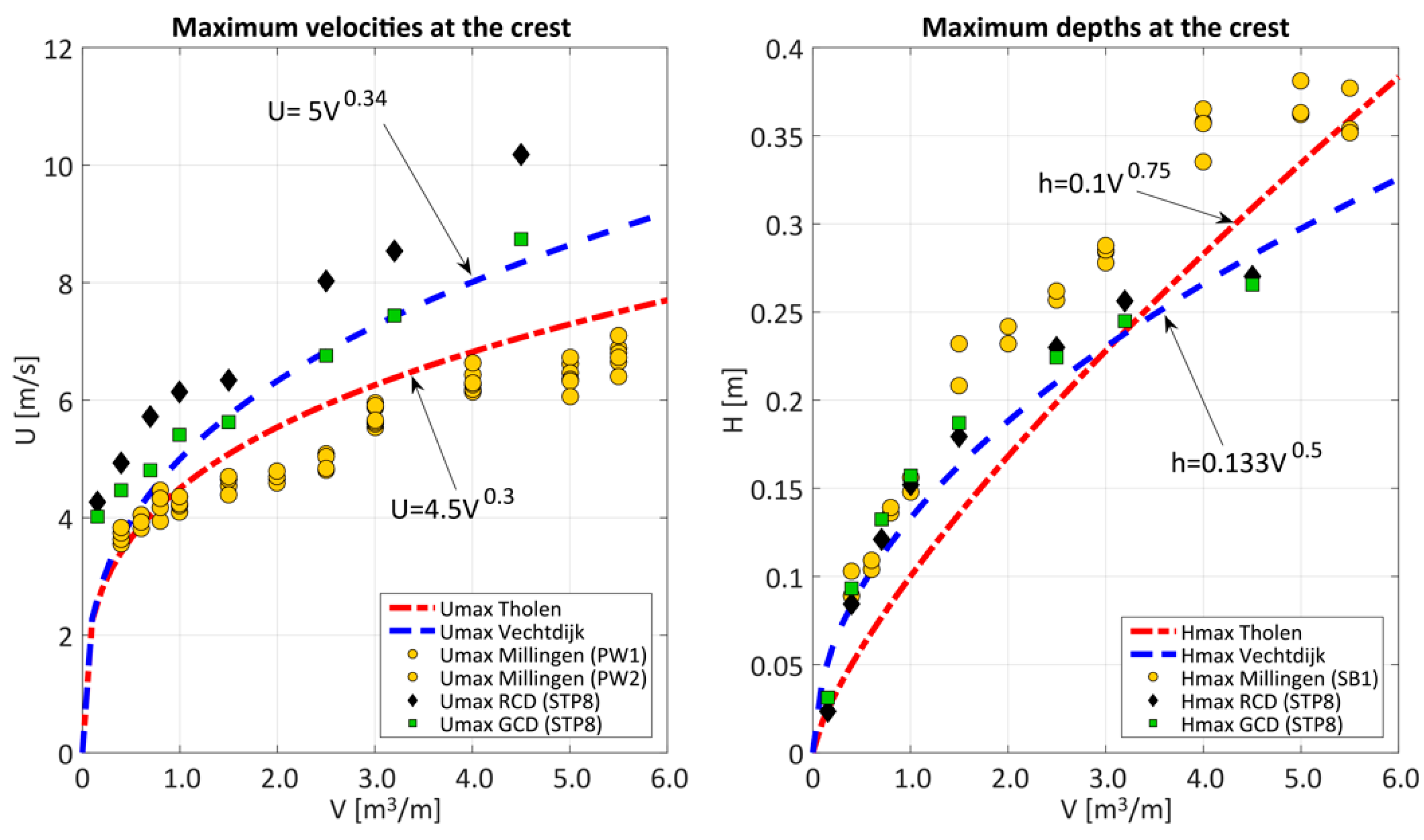
• Local erosion depth is highly influenced by the momentum of the water volume, which is reduced (energy dissipation) by a rough surface such as grass. If a road is present, both the smoother asphalt surface and the resultant bottom irregularities (possibly derived by traffic and material change) increase the scour potential for failure along the crest and the slope with respect to the dike without a road as they influence the generated and dissipated turbulence (kinetic energy) and its variability (turbulence intensities).

Finally, the coupled emulator-erosion model was able to yield realistic probabilities and trends, given all uncertainties in the modelling process. Yet, further improvements are required, especially for the CFD model validation, grass quality estimation, and erosion modelling. The present method can be extended by including model uncertainty coefficients as stochastic variables, to account for the errors originated from the imperfection of both the erosion and the hydrodynamic models. This is especially important to improve the erosion estimation of wave volumes located in the tail of the distribution.

References

- Aguilar-López, J.P. Probabilistic Safety Assessment of Multi-Functional Flood Defences; Twente University: Enschede, The Netherlands, 2016. [Google Scholar]
- Hemer, M.A.; Fan, Y.; Mori, N.; Semedo, A.; Wang, X.L. Projected changes in wave climate from a multi-model ensemble. Nat. Clim. Chang. 2013, 3, 471–476. [Google Scholar] [CrossRef]
- Stocker, T.F.; Qin, D.; Plattner, G.-K.; Alexander, L.V.; Allen, S.K.; Bindoff, N.L.; Bréon, F.-M.; Church, J.A.; Cubasch, U.; Emori, S. Technical summary. In Climate Change 2013: The Physical Science Basis. Contribution of Working Group I to the Fifth Assessment Report of the Intergovernmental Panel on Climate Change; Cambridge University Press: Cambridge, UK, 2013; pp. 33–115. [Google Scholar]
- Middelkoop, H.; Daamen, K.; Gellens, D.; Grabs, W.; Kwadijk, J.C.; Lang, H.; Parmet, B.W.; Schädler, B.; Schulla, J.; Wilke, K. Impact of climate change on hydrological regimes and water resources management in the rhine basin. Clim. Chang. 2001, 49, 105–128. [Google Scholar] [CrossRef]
- Ranasinghe, R.; Callaghan, D.; Stive, M.J. Estimating coastal recession due to sea level rise: Beyond the bruun rule. Clim. Chang. 2012, 110, 561–574. [Google Scholar] [CrossRef]
- Jongejan, R.; Ranasinghe, R.; Wainwright, D.; Callaghan, D.P.; Reyns, J. Drawing the line on coastline recession risk. Ocean Coast. Manag. 2016, 122, 87–94. [Google Scholar] [CrossRef]
- Naulin, M.; Kortenhaus, A.; Oumeraci, H. Reliability-based flood defense analysis in an integrated risk assessment. Coast. Eng. J. 2015, 57. [Google Scholar] [CrossRef]
- Vrijling, J.K. Probabilistic design of water defense systems in the netherlands. Reliabil. Eng. Syst. Saf. 2001, 74, 337–344. [Google Scholar] [CrossRef]
- Lee, C.-E.; Kwon, H.J. Reliability analysis and evaluation of partial safety factors for random wave overtopping. KSCE J. Civ. Eng. 2009, 13. [Google Scholar] [CrossRef]
- Victor, L.; Van der Meer, J.W.; Troch, P. Probability distribution of individual wave overtopping volumes for smooth impermeable steep slopes with low crest freeboards. Coast. Eng. 2012, 64, 87–101. [Google Scholar] [CrossRef]
- Van der Meer, J.W. Technical Report Wave Run-Up and Wave Overtopping at Dikes; Rijkswaterstaat, DWW: Utrecht, The Netherlands, 2002. [Google Scholar]
- Pullen, T.; Allsop, N.; Bruce, T.; Kortenhaus, A.; Sch, H.; Van der Meer, J. Eurotop: Wave Overtopping of Sea Defences and Related Structures: Assessment Manual; Environment Agency: Bristol, UK, 2007.
- Franco, L.; De Gerloni, M.; Van der Meer, J. Wave overtopping on vertical and composite breakwaters. Coast. Eng. Proc. 1994. [Google Scholar] [CrossRef]
- Dean, R.G.; Rosati, J.D.; Walton, T.L.; Edge, B.L. Erosional equivalences of levees: Steady and intermittent wave overtopping. Ocean Eng. 2010, 37, 104–113. [Google Scholar] [CrossRef]
- Van der Meer, J.W.; Hardeman, B.; Steendam, G.J.; Schuttrumpf, H.; Verheij, H.J. Flow depths and velocities at crest and landward slope of a dike, in theory and with the wave overtopping simulator. Coast. Eng. Proc. 2010, 1. [Google Scholar] [CrossRef]
- Steendam, G.J.; Van Hoven, A.; Van der Meer, J.; Hoffmans, G. Wave overtopping simulator tests on transitions and obstacles at grass covered slopes of dikes. Coast. Eng. Proc. 2014, 1. [Google Scholar] [CrossRef]
- Hoffmans, G.J.C.M.; van Hoven, A.; Harderman, B.; Verheij, H. Erosion of grass covers at transitions and objects on dikes. In Proceedings of the 7th International Conference on Scour and Erosion, Perth, Australia, 2–4 December 2015; Cheng, L., Drapper, S., An, H., Eds.; Taylor and Francis Group: Perth, Australia, 2015. [Google Scholar]
- Hoffmans, G.J.C.M.; Akkerman, G.J.; Verheij, H.; Van Hoven, A.; Van der Meer, J. The erodibility of grassed inner dike slopes against wave overtopping. ASCE 2008, 3224–3236. [Google Scholar] [CrossRef]
- Verheij, H.J.; Meijer, D.G.; Kruse, G.A.M.; Smith, G.M.; Vesseur, M. Onderzoek Naar de Sterkte van Graszoden van Rivierdijken; Deltares (WL): Delft, The Netherlands, 1995. [Google Scholar]
- Hewlett, H.; Boorman, L.A.; Bramley, L. Design of Reinforced Grass Waterways; Construction Industry Research and Information Association: London, UK, 1987. [Google Scholar]
- Trung, L. Overtopping on Grass Covered Dikes: Resistance and Failure of the Inner Slopes; TU Delft, Delft University of Technology: Delft, The Netherlands, 2014. [Google Scholar]
- Schüttrumpf, H.; Oumeraci, H. Layer thicknesses and velocities of wave overtopping flow at seadikes. Coast. Eng. 2005, 52, 473–495. [Google Scholar] [CrossRef]
- Kobayashi, N.; Weitzner, H. Erosion of a seaward dike slope by wave action. J. Waterw. Port Coast. Ocean Eng. 2014, 141. [Google Scholar] [CrossRef]
- Quang, T.T.; Oumeraci, H. Numerical modelling of wave overtopping-induced erosion of grassed inner sea-dike slopes. Nat. Hazards 2012, 63, 417–447. [Google Scholar] [CrossRef]
- Ribberink, J.S. Bed-load transport for steady flows and unsteady oscillatory flows. Coast. Eng. 1998, 34, 59–82. [Google Scholar] [CrossRef]
- Bomers, A.; Lopez, J.A.; Warmink, J.J.; Hulscher, S.J. Modelling effects of an asphalt road at a dike crest on dike cover erosion onset during wave overtopping. Nat. Hazards 2018, 1–30. [Google Scholar] [CrossRef]
- Castelletti, A.; Galelli, S.; Ratto, M.; Soncini-Sessa, R.; Young, P.C. A general framework for dynamic emulation modelling in environmental problems. Environ. Model. Softw. 2012, 34, 5–18. [Google Scholar] [CrossRef]
- Razavi, S.T.; Bryan, A.; Burn Donald, H. Review of surrogate modeling in water resources. Water Resour. Res. 2012, 48. [Google Scholar] [CrossRef] [Green Version]
- Duncan, A.; Chen, A.S.; Keedwell, E.; Djordjevic, S.; Savic, D. Urban Flood Prediction in Real-Time from Weather Radar and Rainfall Data Using Artificial Neural Networks; International Association of Hydrological Sciences: Exeter, UK, 2011. [Google Scholar]
- Aguilar-Lopez, J.P.; Van Andel, S.J.; Werner, M.; Solomatine, D.P. Hydrodynamic and water quality surrogate modelling for reservoir operation. In Proceedings of the 11th IWA/IAHR International Conference on Hydroinformatics, New York, NY, USA, 17–21 August 2014. [Google Scholar]
- Kingston, G.B.; Rajabalinejad, M.; Ben, P.G.; Van Gelder, P.H.A.J.M. Computational intelligence methods for the efficient reliability analysis of complex flood defence structures. Struct. Saf. 2011, 33, 64–73. [Google Scholar] [CrossRef]
- Aguilar-López, J.P.; Warmink, J.J.; Schielen, R.M.J.; Hulscher, S.J.M.H. Data-driven surrogate models for flood defence failure estiamtion: “Jarillon de calí”. In Proceedings of the 11th IWA/IAHR International Conference on Hydroinformatics, New York, NY, USA, 17–21 August 2014. [Google Scholar]
- Aguilar-López, J.P.; Warmink, J.J.; Schielen, R.M.J.; Hulscher, S.J.M.H. Piping erosion safety assessment of flood defences founded over sewer pipes. Eur. J. Environ. Civ. Eng. 2016, 1–29. [Google Scholar] [CrossRef]
- Van Gent, M.R.A.; van den Boogaard, H.F.P.; Pozueta, B.; Medina, J.R. Neural network modelling of wave overtopping at coastal structures. Coast. Eng. 2007, 54, 586–593. [Google Scholar] [CrossRef]
- Bomers, A.; Aguilar-López, J.P.; Warmink, J.J.; Hulscher, S.J.M.H. Modelling erosion development during wave overtopping of an asphalt road covered dike. In Proceedings of the FLOODrisk 2016 3rd European Conference on Flood Risk Management, Innovation, Implementation and Integration, Lyon, France, 16–21 October 2016. [Google Scholar]
- Hoffmans, G.J.C.M. The Influence of Turbulence on Soil Erosion; Eburon Uitgeverij BV: Delft, The Netherlands, 2012. [Google Scholar]
- Hughes, S.A. Adaptation of the Levee Erosional Equivalence Method for the Hurricane Storm Damage Risk Reduction System (Hsdrrs); DTIC Document: Fort Belvoir, VA, USA, 2011. [Google Scholar]
- Partheniades, E. Erosion and deposition of cohesive soils. J. Hydraul. Div. 1965, 91, 105–139. [Google Scholar]
- Verheij, H.J.; Hoffmans, G.J.C.M.; van der meer, J. Evaluation and Model Development, Grass Erosion Test at the Rhine Dike; Deltares: Delft, The Netherlands, 2015. [Google Scholar]
- Launder, B.E.; Spalding, D.B. The numerical computation of turbulent flows. Comput. Methods Appl. Mech. Eng. 1974, 3, 269–289. [Google Scholar] [CrossRef]
- COMSOL. The Comsol CFD Module User's Guide (Version 5.2); COMSOL: Stockholm, Sweden, 2015. [Google Scholar]
- Marriott, M.J.; Jayaratne, R. Hydraulic Roughness–Links Between Manning’s Coefficient, Nikuradse’s Equivalent Sand Roughness and Bed Grain Size; UEL: London, UK, 2010. [Google Scholar]
- Te Chow, V. Open Channel Hydraulics; McGraw-Hill: London, UK, 1959. [Google Scholar]
- Jansen, R.B. Advanced dam Engineering for Design, Construction, and Rehabilitation; Springer Science & Business Media: Berlin/Heidelberg, Germany, 2012. [Google Scholar]
- Bakker, J.; Melis, R.; Mom, R. Factual Report: Overslagproeven Rivierenland; INFRAM: Dutch, The Netherlands, 2013. [Google Scholar]
- Van der Meer, J.W.; Van Hovern, A.; Paulissen, M.; Steendam, G.J.; Verheij, H.J.; Hoffmans, G.J.C.M.; Kruse, G.A.M. Handreiking Toetsen Grasbekledingen op Dijken TBV Het Opstellen van het Beheerdersoordeel (bo) in de Verlengde Derde Toetsronde; Rijkswaterstaat, Waterdienst: Utrecht, The Netherlands, 2012. [Google Scholar]
- Forrester, A.; Sobester, A.; Keane, A. Engineering Design via Surrogate Modelling: A Practical Guide; John Wiley & Sons: Hoboken, NJ, USA, 2008. [Google Scholar]
- Piontkowitz, T. Erograss: Failure of Grass Cover Layers at Seaward and Shoreward Dike Slopes. Design, Construction and Performance; Danish Coastal Inspectorate: Copenhagen, Denmark, 2009. [Google Scholar]
- Van der Meer, J.W.; Janssen, J.; Hydraulics, D. Wave Run-Up and Wave Overtopping at Dikes and Revetments; Delft Hydraulics: Delft, The Netherlands, 1994. [Google Scholar]
- Hughes, S.A.; Thornton, C.I.; Van der Meer, J.W.; Scholl, B.N. Improvements in describing wave overtopping processes. Coast. Eng. Proc. 2012, 1. [Google Scholar] [CrossRef]
- Van Loon-Steensma, J.M.; Vellinga, P. Robust, multifunctional flood defenses in the dutch rural riverine area. Nat. Hazards Earth Syst. Sci. 2014, 14, 1085–1098. [Google Scholar] [CrossRef]