Experimental Validation of Fluid–Structure Interaction Computations of Flexible Composite Propellers in Open Water Conditions Using BEM-FEM and RANS-FEM Methods

Abstract

In the past several decades, many papers have been published on fluid–structure coupled calculations to analyse the hydro-elastic response of flexible (composite) propellers. The flow is usually modelled either by the Navier–Stokes equations or as a potential flow, by assuming an irrotational flow. Phenomena as separation of the flow, flow transition, boundary layer build-up and vorticity dynamics are not captured in a non-viscous potential flow. Nevertheless, potential flow based methods have been shown to be powerful methods to resolve the hydrodynamics of propellers. With the upcoming interest in flexible (composite) propellers, a valid question is what the consequences of the potential flow simplifications are with regard to the coupled fluid–structure analyses of these types of propellers. This question has been addressed in the following way: calculations and experiments were conducted for uniform flows only, with a propeller geometry that challenges the potential flow model due to its sensitivity to leading edge vortex separation. Calculations were performed on the undeformed propeller geometry with a Reynolds-averaged-Navier–Stokes (RANS) solver and a boundary element method (BEM). These calculations show some typical differences between the RANS and BEM results. The flexible propeller responses were predicted by coupled calculations between BEM and finite element method (FEM) and RANS and FEM. The applied methodologies are briefly described. Results obtained from both calculation methods have been compared to experimental results obtained from blade deformation measurements in a cavitation tunnel. The results show that, even for the extreme cases, promising results have been obtained with the BEM-FEM coupling. The BEM-FEM calculated responses are consistent with the RANS-FEM results.

1. Introduction

In the last several decades, many papers have been published on the hydro-elastic analysis of flexible (composite) propellers. The majority of the studies were limited to steady inflow conditions. In these studies, mainly three different approaches were used for the hydrodynamic calculations of flexible propellers viz. Reynolds averaged Navier–Stokes methods (RANS), boundary element methods (BEM) and vortex lattice methods (VLM). In BEM and VLM computations, the flow is assumed to be a potential flow.

RANS solvers were used in the flexible propeller FSI computations presented in [1,2,3,4]. BEM solvers were applied in the hydro-elastic propeller analysis as presented in [5,6,7,8,9,10,11,12]. In the hydro-elastic coupling, procedures presented in [13,14] VLM solvers were applied.

The fundamental difference between RANS computations and potential flow based calculations is that phenomena as separation of the flow, flow transition, boundary layer build-up and vorticity dynamics are not modelled in the latter one. For rigid propellers, the consequences of these flow simplifications have been studied in the past. Results of such studies were presented in the proceedings of the first and fourth Symposium on Marine Propulsors, for instance. These proceedings include papers with results of comparative studies with different RANS and BEM calculations together with experimental results for rigid propellers [15,16]. Around the optimum efficiency, a good agreement between BEM, RANS and experimental results is obtained. An increasing inaccuracy of the BEM results can be expected for larger skew angles and smaller advance coefficients [12]. This is explained by the increased leading edge vortex strength for decreasing advance ratios and increasing skew angles. This indicates that, for blade integrated values like thrust and torque, vorticity phenomena may not be negligible for high loading conditions and propellers with considerable skew. However, comparative studies between RANS and potential flow based hydro-elastic calculations for flexible propellers are still lacking.

Recently, the influence of viscous effects on the hydro-elastic response of hydrofoils has been investigated [17,18]. It has been shown that the flow-induced bend-twist coupling effects of a flexible hydrofoil in fully turbulent and attached flow conditions are well predicted with an inviscid fluid–structure interaction (FSI) method [17]. However, when the stability boundaries are reached (i.e., static/dynamic divergence or flutter velocity boundaries), viscous FSI methods were recommended to predict the dynamic response, especially for solid-to-fluid added mass ratios smaller than four [18]. Therefore, it is expected that, for uniform flow conditions, in which dynamic instabilities are irrelevant, an accurate prediction of the FSI response of marine propellers can be obtained with an inviscid method when the flow is fully turbulent and attached.

However, both conditions are not met for the small scale propellers considered in this work. Measurements and calculations have been performed at a transitional flow regime, partly laminar and partly turbulent. Secondly, experiments have been conducted at relatively high angles of attack resulting in a leading edge vortex and flow separation at the trailing edge. Finally, due to the finite blade size, a vortex is generated at the blade tips. The influence of these viscous effects and vorticity phenomena on the hydro-elastic response prediction is not known. Therefore, experimental and RANS-FEM results have been used to validate a BEM-FEM coupled calculation for uniform flows.

The main purpose of this paper is to validate the RANS-FEM and BEM-FEM coupled calculations with experimental results and to show what the consequences of the potential flow simplifications are with regard to the coupled fluid–structure response. This work is structured as follows: first, the different propellers are described in Section 2. Section 3 provides information about the structural modelling. In Section 4, the fluid models are explained. The BEM-FEM and RANS-FEM coupling are described in Section 5. Section 6 presents a comparison of open water measurements and BEM and RANS calculations for a rigid propeller. In Section 7, the cavitation tunnel experiments are explained. Section 8 presents an uncertainty estimation for measurements and RANS-FEM and BEM-FEM calculations. In Section 9, the experimental results obtained for the flexible propellers are compared to results obtained with the BEM-FEM and RANS-FEM coupling. Conclusions and recommendations are given in Section 10.

2. General Description of Propellers and Flow Conditions

2.1. Propellers

Four propellers are considered. The propellers have a diameter (D) of 0.34 m and are similar in size and geometry, but differ with respect to blade material. Two propellers are made out of glass fibre reinforced epoxy with different laminate orientations. The other two propellers are made of isotropic material: one bronze propeller and one made of epoxy. The propellers have been labelled as follows:

• Propeller bronze: this propeller is assumed completely rigid.
• Propeller epoxy: this propeller is the most flexible one.
• Propeller 45: [+45${}^{°}$/−45${}^{°}$] laminate lay-up.
• Propeller 90: [0${}^{°}$/90${}^{°}$] laminate lay-up.

The 0${}^{°}$-direction of the laminae is parallel to the z-axis of the propeller blade coordinate system, where positive x-, y- and z-axis are pointing forward, portside and upwards, respectively. All the results are presented according to this coordinate system.

2.2. Material Properties

The Young’s moduli E, Poisson ratios $\upsilon$ and the shear moduli G of the epoxy material and the composite laminate are given in

Table 1. Elastic properties of epoxy.

E (GPa)	$\mathit{\upsilon }$ (-)	G (GPa)
3.60	0.300	1.39

and

Table 2. Composite [0${}^{°}$/90${}^{°}$] laminate elastic properties.

${\mathit{E}}_{\mathbf{11}}$ (GPa)	${\mathit{E}}_{\mathbf{22}}$ (GPa)	${\mathit{E}}_{\mathbf{33}}$ (GPa)	${\mathit{\upsilon }}_{\mathbf{12}}$ (-)	${\mathit{\upsilon }}_{\mathbf{13}}$ (-)	${\mathit{\upsilon }}_{\mathbf{23}}$ (-)	${\mathit{G}}_{\mathbf{12}}$ (GPa)	${\mathit{G}}_{\mathbf{13}}$ (GPa)	${\mathit{G}}_{\mathbf{23}}$ (GPa)
18.8	18.8	8.00	0.132	0.275	0.275	2.81	2.49	2.49

.

2.3. Flow Conditions

For the open water calculations, computations have been performed for a constant rotational speed (n) of 1170 rpm and varying advance speed, keeping the Reynolds number as constant as possible for different flow conditions.

The flexible propeller calculations have been performed for the measured conditions with advance ratios around 0.37, 0.64 and 0.85 as given in

Table 3. Flow conditions for the flexible propeller calculations and measurements.

	$\mathit{J}\mathbf{=}\frac{\mathbf{60}\mathit{v}}{\mathit{nD}}$	v (m/s)	n (rpm)	${\mathit{Re}}_{\mathbf{0.7}\mathit{r}}\mathbf{\times }{\mathbf{10}}^{\mathbf{6}}$
Prop. Epoxy, blade 1	0.37	1.88	900	1.28
Prop. Epoxy, blade 1	0.64	3.97	1098	1.60
Prop. Epoxy, blade 1	0.85	6.73	1392	2.10
Prop. 45, blade 1	0.38	1.92	900	1.28
Prop. 45, blade 1	0.64	3.99	1098	1.60
Prop. 45, blade 1	0.85	6.75	1398	2.10
Prop. 90, blade 2	0.38	1.98	900	1.28
Prop. 90, blade 2	0.66	4.09	1098	1.60
Prop. 90, blade 2	0.85	6.74	1398	2.10

. All calculations have been performed for uniform inflow conditions. The last column of Table 3 presents the Reynolds number, $Re$, based on the chord length (C) and flow velocity at 0.7 of the propeller radius (r),

$$R{e}_{0.7r}=\frac{\rho C_{0.7r}\sqrt{v^2+{\left(0.7\pi nD\right)}^2}}{\mu },$$

(1)

with $\rho$ the density of water taken as 1000 kgm${}^{-3}$ and $\mu$ the dynamic viscosity equal to 1.01$·{10}^{-3}$ Pa·s.

3. Structure Model

For FEM modelling and computations, MSC Marc/Mentat has been used. The FEM models consist of one propeller blade without the hub part. The stiffness contribution of the hub has been modelled by a full clamping of the propeller blade at the blade–hub interface. The models were discretised by quadratic solid elements. A mesh convergence study has been conducted in order to ensure a mesh independent solution for the calculated displacements. Structured FEM meshes have been used, identified with the following three discretisation parameters: $N_c$ the number of elements in chordwise direction, $N_r$ the number of elements in radial direction and $N_n$ the number of elements in through-thickness direction.

Table 4. Results of finite element method mesh convergence study.

${\mathit{N}}_{\mathit{c}}$	${\mathit{N}}_{\mathit{r}}$	${\mathit{N}}_{\mathit{n}}$	Tip Displ. (mm)
116	120	4	16.76
58	60	4	16.76
58	60	8	16.76
29	30	4	16.74

presents the displacements of the tip for a static load case obtained with FEM models for different meshes.

These results show that, for the $29\times 30\times 4$ element distribution, the tip displacement differs approximately 0.1% from the grid independent solution. Therefore, the $29\times 30\times 4$ element distribution has been used for all the FEM calculations.

In the FEM modelling, special attention has been given to the establishment of the material orientations in composite blades. In [19,20], the importance of a proper material orientation for doubly curved structures has been described. Standard commercial FEM software packages are usually not able to define unambiguously the material orientations in complex geometries [19]. In [20], an approach has been presented to determine the element dependent material orientations in doubly curved structures. In this method, the through thickness direction and the projection of the transverse laminate (90${}^{°}$)-direction on the element surface is used to establish the material orientation per element. A more detailed description of this approach and the blade FEM modelling can be found in that paper.

4. Fluid Models

4.1. BEM Model

For this work, the BEM PROCAL, developed by the Maritime Research Institute Netherlands (MARIN) [21,22] was used. In BEM, only the surfaces of the object have to be discretized. From a grid sensitivity study, it was concluded that a $29\times 30$ element distribution is sufficient to obtain a grid independent solution. In the previous section, it was revealed that, in the FEM model, 29 and 30 elements are distributed along the blade chord and radius, respectively. This means that the BEM and FEM solvers require a similar distribution of panels or elements on the propeller surface. This property has been used by applying identical mesh distributions in the FEM and the BEM model in order to avoid the need for an interpolation of pressure and structural response between the two grids.

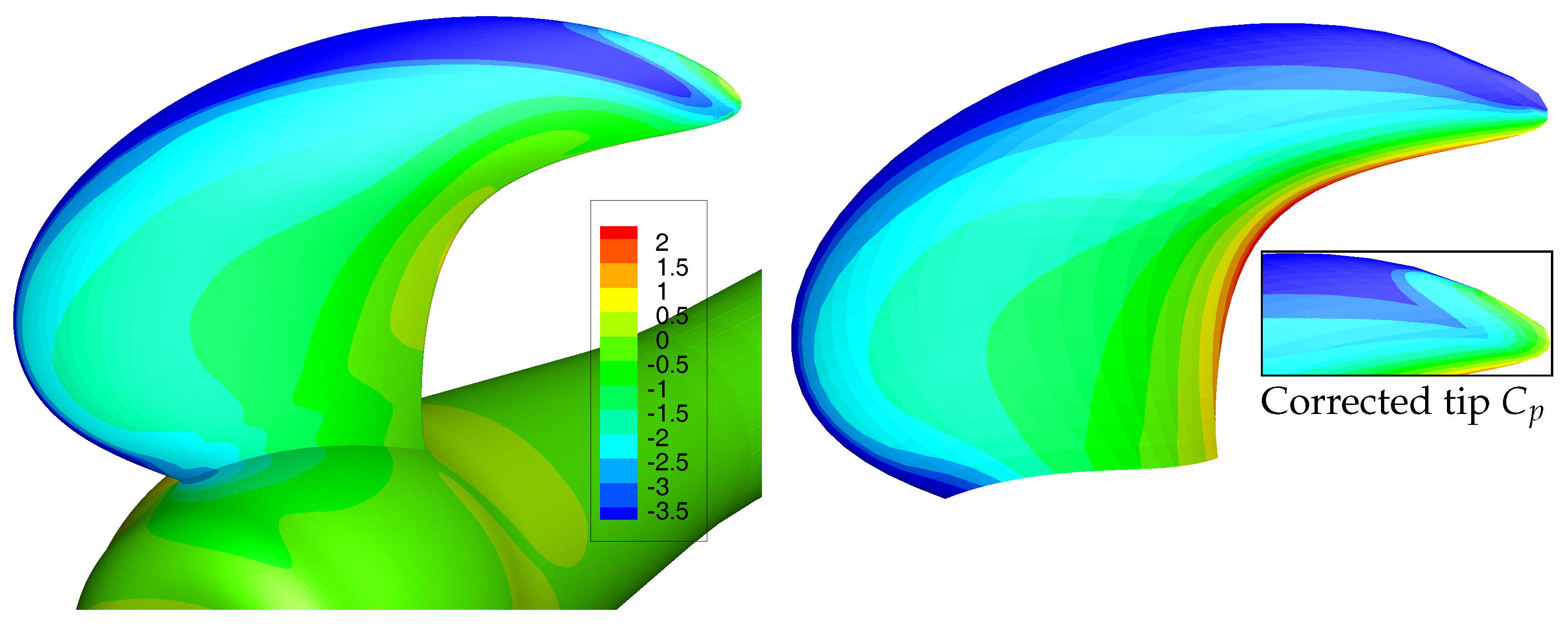
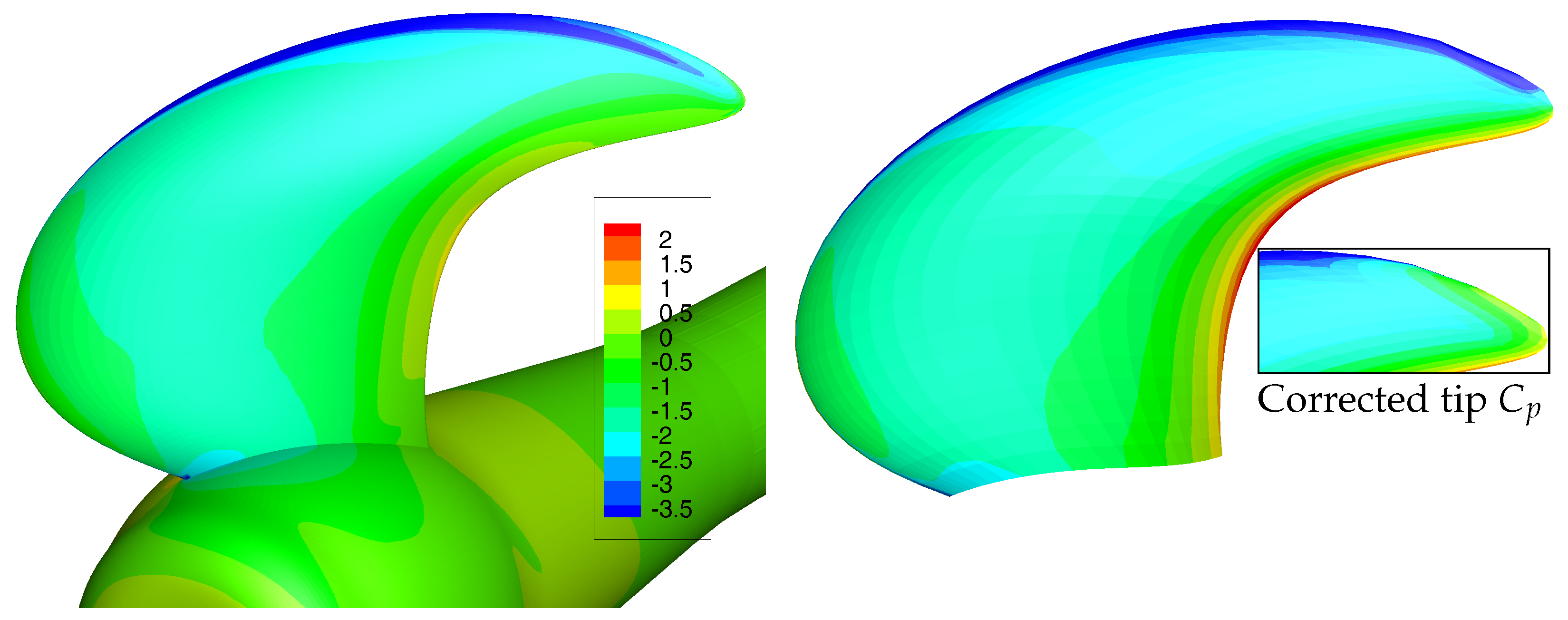
Two corrections are applied on the PROCAL pressures before they are imposed on the FEM model. The first correction is to rectify for an overestimation of the pressures at the propeller tip. In general, with a potential flow solver, a pressure difference between blade face and back at the tip will be computed, while, in reality, this pressure difference will be zero. To correct for this, the calculated pressures from a certain propeller radius are smoothed to a zero pressure coefficient at the tip. The default from where this tip pressure correction is applied is 95% of the propeller radius. This value has been used throughout this work. The pressure smoothing radius has an important influence on the propeller blade deformations at the tip, since the tip is relatively flexible and therefore the tip deformations are sensitive to small changes in pressure distribution [23].

The second correction is a viscous correction to include frictional losses. The viscous shear stresses have been computed using the maximum skin friction coefficient calculated from the Blasius formulation for laminar flow, ITTC formulation for transition to turbulent flow [24] and the Prandtl–Schlichting formulation. The skin friction coefficients have been used to calculate the blade tangential forces from the total velocities and element areas per element. These forces have been imposed on the FEM model.

The correction for the minimum allowable pressure coefficient as explained in Section 6.1.1 has not been used in the BEM-FEM calculations because this correction applies only for the lowest advance ratios of 0.37 and 0.38, but hardly affects the hydro-elastic response for these conditions.

4.2. RANS Model

RANS calculations have been conducted with the CFD software ReFRESCO developed at MARIN. ReFRESCO [25] is a community based open-usage/open-source CFD code for the maritime world. It solves multiphase (unsteady) incompressible viscous flows using the Navier–Stokes equations, complemented with turbulence models, cavitation models and volume-fraction transport equations for different phases. The equations are discretised using a finite-volume approach with cell-centered collocated variables, in strong-conservation form and a pressure-correction equation based on the SIMPLE algorithm is used to ensure mass conservation [26,27].

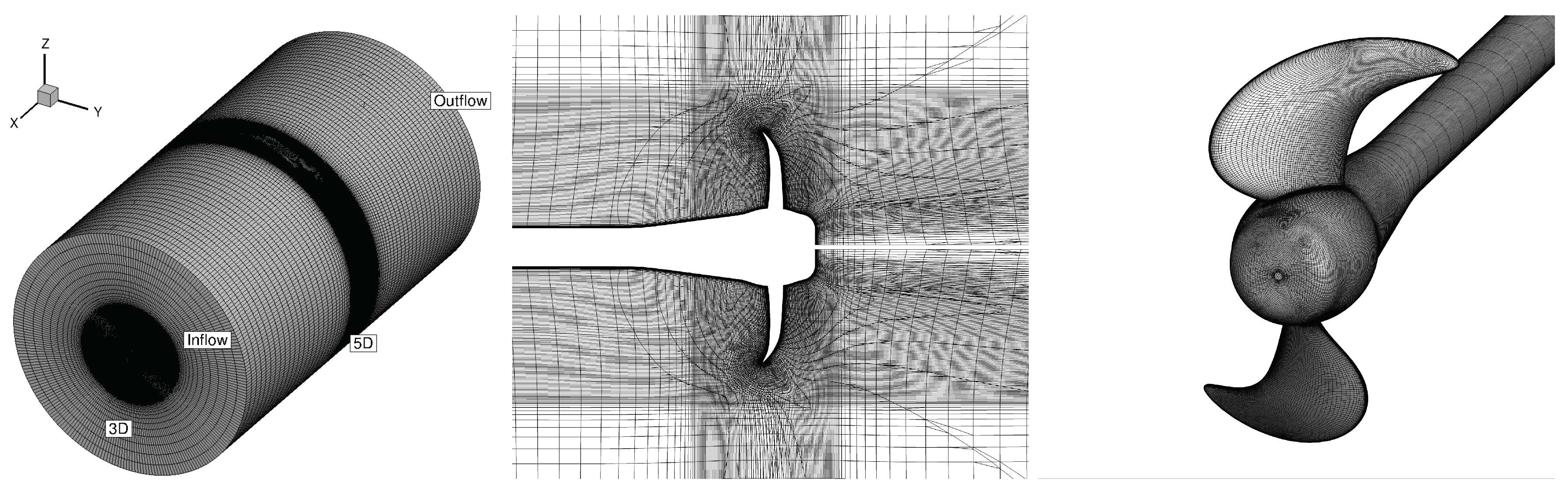
Since open water conditions are considered, the computations can be done using a body fitted, rotating reference system. For this, the propeller has been modelled in a rotating circular domain with diameter and length three and five times the propeller diameter, respectively. The propeller is located in the middle of this domain. The computational domain consists of a structured multi-block grid built with GridPro, using a standard block topology developed at MARIN. The topology is applied quite often and gives good quality grids, most of the time. However, for the propeller considered here, grid generation was cumbersome due to the relatively high skew of the propeller blades, the relatively thin leading edge and propeller section thickness’s. The quality of the grid was not very high, which leads to convergence problems of the solver when using higher order discretisations of the convective fluxes (QUICK scheme). Therefore, for all calculations, a blending between central and upwind discretisation was used. Figures of the domain, grid and propeller are depicted in Figure 1. For all the calculations, the $k-\sqrt{k}L$ turbulence model has been used as described in [28]. The $k-\sqrt{k}L$ turbulence model gives very similar results as the $k-\omega$ SST model, but shows in general an improved iterative convergence. This has been shown explicitly for propeller flows [29].

The boundary conditions applied on the domain and propeller are given in

Table 5. Boundary conditions for Reynolds-averaged-Navier–Stokes calculations.

	Boundary Condition
Inlet	Prescribed inflow velocity.
Inner outlet	Neumann boundary condition on velocity and pressure.
Outer outlet	Dirichlet boundary condition on pressure, Neumann on velocity.
Propeller, hub and shaft surfaces	Velocity is zero, no wall functions applied (y+ should be <1).
Outer surface flow domain	Normal and tangential velocity are zero and free, respectively.

. At the inlet, the velocity is imposed. At the outlet, a combination of an outflow and pressure condition is imposed. Behind the propeller, the velocity derivatives are imposed to be zero; at the remainder of the outlet, the pressure is imposed. The propeller, hub and shaft have a no-slip boundary condition. In the calculations, no wall functions have been used, i.e., in all calculations, the non-dimensional wall distance y+ was below 1. At the outer surface of the circular domain, a free-slip boundary condition is applied, i.e., the velocities normal to the surface are zero and the tangential velocities are free.

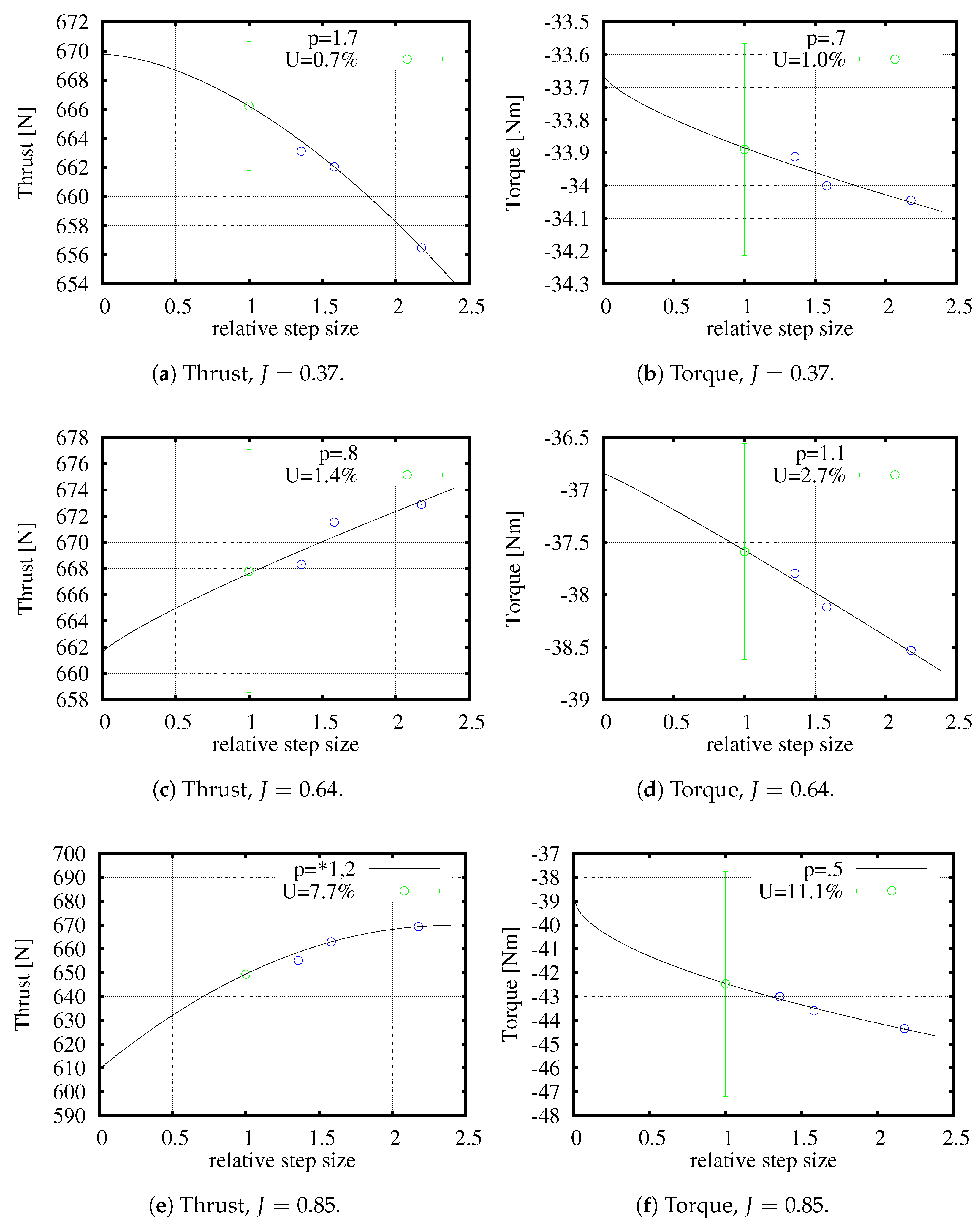
Thrust and Torque RANS Discretisation Uncertainties

The discretisation errors in the thrust and torque values obtained with the RANS calculations have been estimated with the method described in [30]. In this approach, the numerical uncertainty is obtained using solutions on systematically refined grids. The error is estimated with power series expansions as a function of the typical cell size. The expansions are fitted to the data in the least-squares sense. For the present uncertainty estimation, four grids with cell densities described in

Table 6. Amount of cells and relative step size for different grids.

Grid	Amount of Cells	Relative Step Size
A	917,000	2.18
B	2,390,000	1.58
C	3,790,000	1.36
D	9,460,000	1.00

have been used. The third row gives the relative step size. This parameter identifies the representative grid cell size and is the cubic root of the ratio between the amount of grids cells for finest grid and the considered grid.

Figure 2 shows the results of the discretisation uncertainty quantification for the thrust and torque values computed for the three advance coefficients. The figures show that the order of accuracy p is in the range 0.5 to 1.7. $p=\ast 1,2$ means that a fit was made using first and second order exponents. The order of accuracy is smaller than the typical value of two that would have been obtained when a quadratic upwind differencing (QUICK) scheme was used for the convective flux discretisation. However, with a QUICK scheme, the computations did not converge.

The results show that the discretisation uncertainties are small (<3%) for the advance ratios 0.37 and 0.64. The uncertainties are the highest for the largest advance coefficient, 7.7% and 11.2% for the thrust and torque, respectively. These values are higher than generally accepted. Therefore, for the advance ratio of 0.85, a computation has been performed with a further refined grid. Unfortunately, this calculation required a smaller blending factor to converge and therefore it was decided to stay with grid D.

5. Fluid–Structure Coupling

5.1. BEM-FEM Coupling

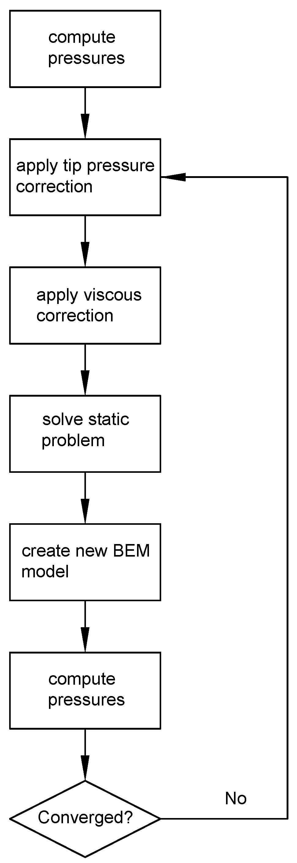
Figure 3 shows the coupling procedure between the BEM solver PROCAL and the FEM software MSC Marc. In this coupling, the following nonlinear equation is solved:

$$\mathbf{K}\mathbf{u}={\mathbf{f}}_{BEM}\left(\mathbf{u}\right)+{\mathbf{f}}_{viscous}\left(\mathbf{u}\right)+{\mathbf{f}}_{centrifugal},$$

(2)

where ${\mathbf{f}}_{BEM}$, ${\mathbf{f}}_{viscous}$ and ${\mathbf{f}}_{centrifugal}$ denote potential flow force, viscous forces and centrifugal forces, respectively. $\mathbf{K}$ is the stiffness matrix. Essentially, all the variables in Equation (2) are a function of the deformations $\mathbf{u}$. Since the blade deformations are relatively small, geometric linear elastic analyses are performed with the FEM solver and therefore the stiffness matrix and centrifugal force vector are not functions of $\mathbf{u}$.

The first step in the coupled BEM-FEM calculation is a PROCAL calculation on the undeformed geometry. The tip pressure correction is applied on the pressures obtained with PROCAL as explained above. Next, the viscous forces are calculated to account for frictional losses. Subsequently, the calculated pressures and viscous forces are used to calculate the structural response of the propeller blade. The structural deformations are used to construct a new propeller geometry from which new fluid pressures are calculated. When not converged, the iteration loop starts again.

5.2. RANS-FEM Coupling

Recently, MARIN has developed an FSI module in ReFRESCO, the implementation and a verification study have been presented in [31]. The method is a partitioned strong coupling approach, meaning that the fluid and structural problem are solved separately and coupling iterations are performed each timestep to obtain the coupled solution. To stabilize this procedure under-relaxation is applied by means of the Aitken adaptive under-relaxation method. For transfer of information across the fluid–structure interface, a radial basis-function (RBF) interpolation is used.

In [31], a verification study was presented for the unsteady problem of the flow around a rigid cylinder with a flexible flap (the Turek benchmark [32]). Results obtained with the FSI module of ReFRESCO were in good agreement with results presented in literature.

The FSI module has been developed for unsteady FSI problems. For steady FSI problems, like the flow around a flexible propeller in open water conditions, the FSI module can be used by performing unsteady simulations until equilibrium is obtained. This was applied in this work, since only open water conditions have been considered. For steady FSI problems the equilibrium solution should be irrespective of the time step in the RANS and FEM calculation, which was the case for all the computations. The most convenient was to apply the same time step in RANS and FEM calculation.

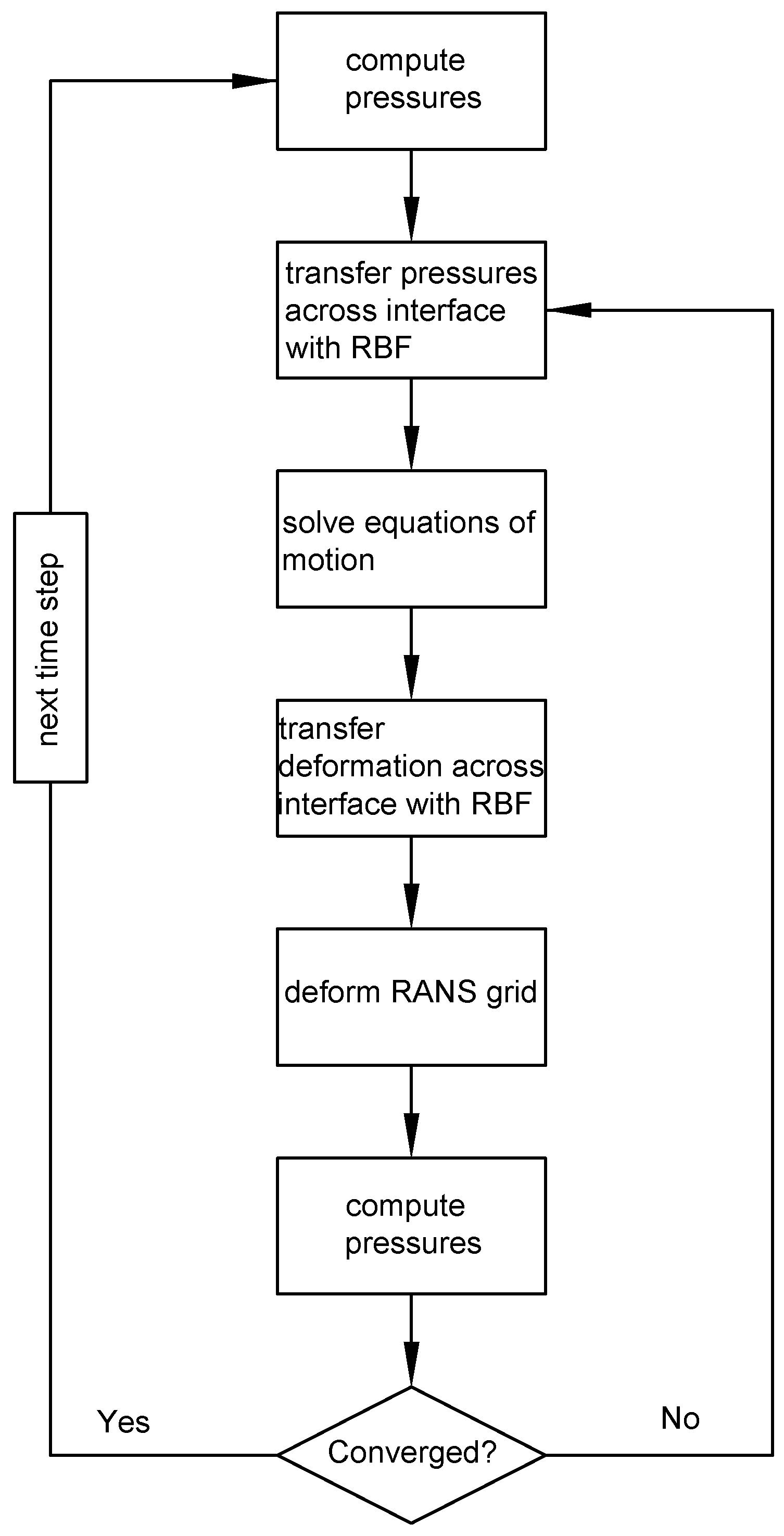
Figure 4 shows the flow chart for one time step with the RANS-FEM coupling. Each time step starts with a RANS computation. Then, the pressures are transferred to the FEM calculation by using an RBF interpolation. With FEM, the structural response is computed. Subsequently, the structural response is transferred to the RANS calculation by again using an RBF interpolation. Based on the blade deformations, the RANS grid is adapted and the pressures are recomputed until convergence is obtained. Then, the following time step is resolved in the same way. For the steady problems considered in this work, the RANS-FEM calculation runs through a number of time steps until the steady state solution is obtained.

6. Comparison of Experimental, BEM and RANS Results for the Bronze Propeller

6.1. Open Water Diagram Bronze Propeller

The open water diagram of the bronze propeller has been measured and compared to calculated open water diagrams with PROCAL and ReFRESCO. Open water measurements have been performed in the deepwater towing tank of MARIN at a constant rotational speed of 1170 rpm and varying advance speed. The Reynolds number based on velocity and chord length at 0.7 of the propeller radius then varies between $1.64\times {10}^6$ and $1.90\times {10}^6$. A total measurement uncertainty (precision and bias) of 3% on thrust and torque can be adopted for these measurements.

6.1.1. Comparison of Experimental and BEM Results

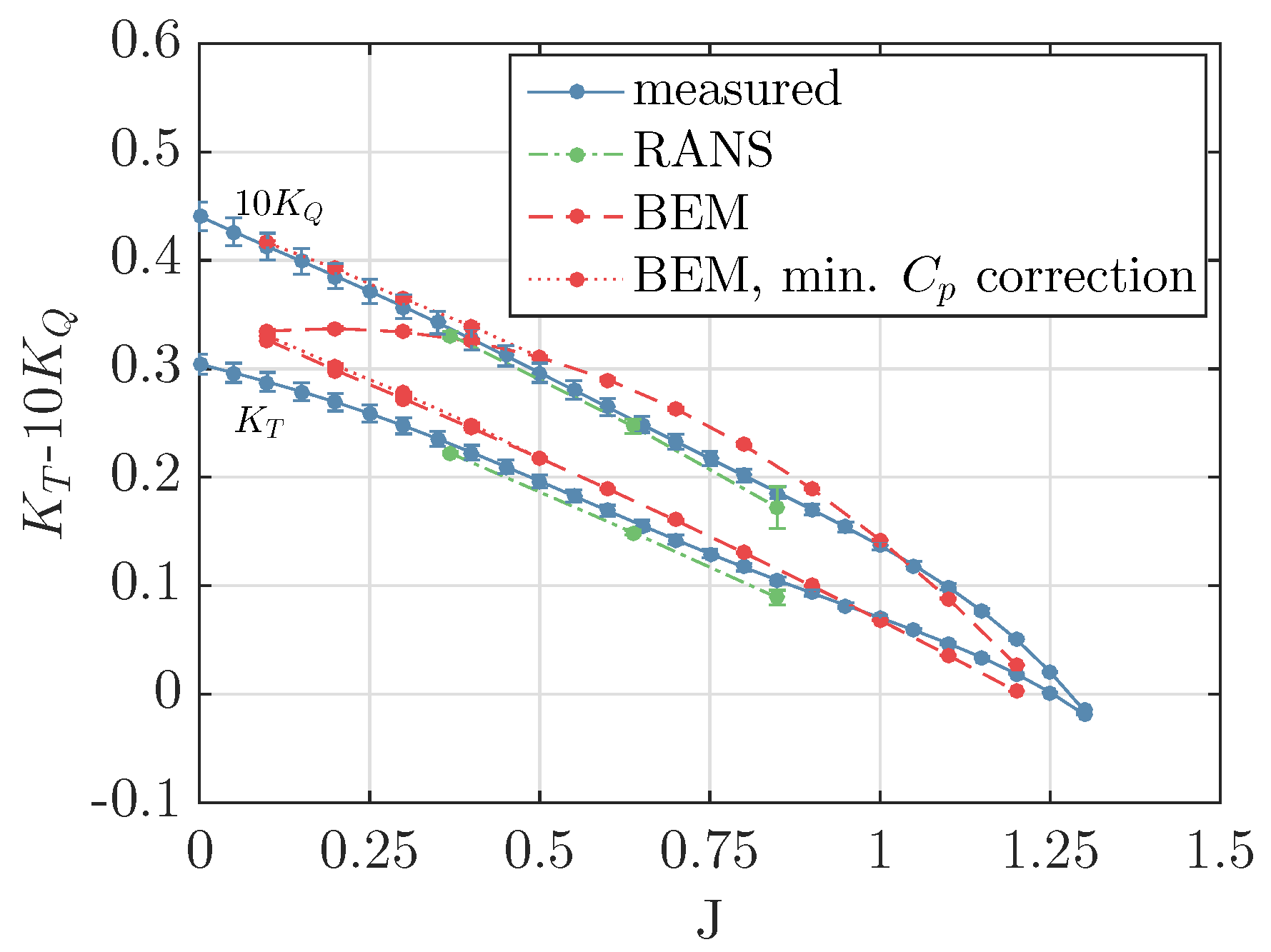
For the BEM calculations, a discretisation error of 0.5% in thrust and torque is estimated by taking the percentage difference between the mesh independent thrust and torque values and the values obtained for the considered panel distribution. The measured and calculated open water curves are depicted in Figure 5 with their uncertainty bands. Particularly for $J<0.4$ and $J>1$, a relatively large discrepancy between measured and calculated curves is seen, especially for the torque coefficient. For $J>1$, viscous effects play an increasingly important role and therefore the results of the PROCAL calculations diverge from the measured results. The discrepancy for low advance coefficients is attributed to the relatively sharp leading edge the potential flow modelling. This results, for heavy loading conditions, in unrealistic high flow velocities and consequently low pressures at the leading edge, since the flow does not separate in the BEM calculation. In reality, the flow will separate, which will limit the suction pressure. The torque is mainly affected by the unrealistic low pressures at the leading edge because the surface normals at the leading edge point mainly in the direction of the blade nose-tail line and therefore the low leading edge pressures reduce the drag rather than the lift. A correction on the suction pressures can be applied by restricting the minimum pressure coefficient, $C_p$, obtained with the BEM calculation by replacing lower pressures with that value. By properly selecting the minimum allowable pressure coefficient for the different advance ratios, the dotted $KQ$ curve of Figure 5 is obtained. For $J>0.4,$ no minimum pressure correction has been applied.

6.1.2. Comparison of Experimental and RANS Results

The calculated open water coefficients with ReFRESCO together with the discretisation uncertainty bandwidths are depicted in Figure 5 as well. The RANS computed thrust and torque coefficients are smaller than the measured values. The uncertainty bars show that the differences can be explained from uncertainties in the RANS computations and the measurements, except for the highest advance coefficient. That means that, with the present RANS calculation, the thrust and therefore the pressure distribution cannot be correctly resolved for this propeller at $J=0.85$. A plausible explanation for this is the modelling error originating from the turbulence model, while a transition model might be more appropriate. This modelling uncertainty might be significant for this condition, since, for an increasing advance ratio, the lift force decrease and viscous forces become more important.

6.2. Comparison of BEM and RANS Pressure Distributions

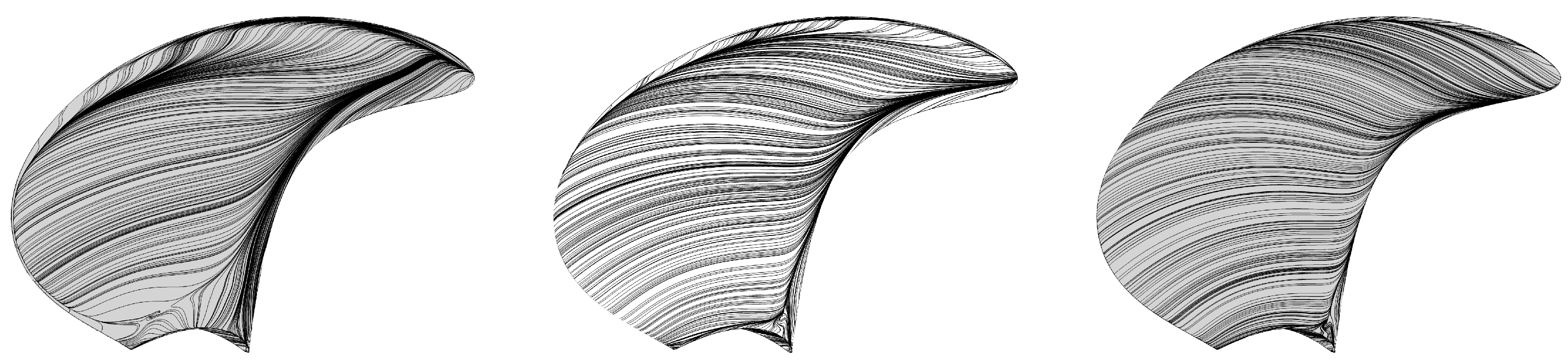
Figure 5 shows significant differences between BEM and RANS results. Not surprisingly, the RANS results seem more accurate than the BEM results, since the RANS calculation includes viscous flow modelling and a vorticity phenomena. To investigate the differences between BEM and RANS results in more detail, pressure distributions obtained with both methods for the first three flow conditions of Table 3 are compared. For these flow conditions, the limiting streamlines on the propeller suction side are depicted in Figure 6. As indicated by the contraction of the streamlines, three flow separation areas can be distinguished: separation at the leading edge resulting in a leading edge vortex, a separation area at the trailing edge and flow separation at the propeller tip. The least flow separation is obtained for the highest advance coefficient.

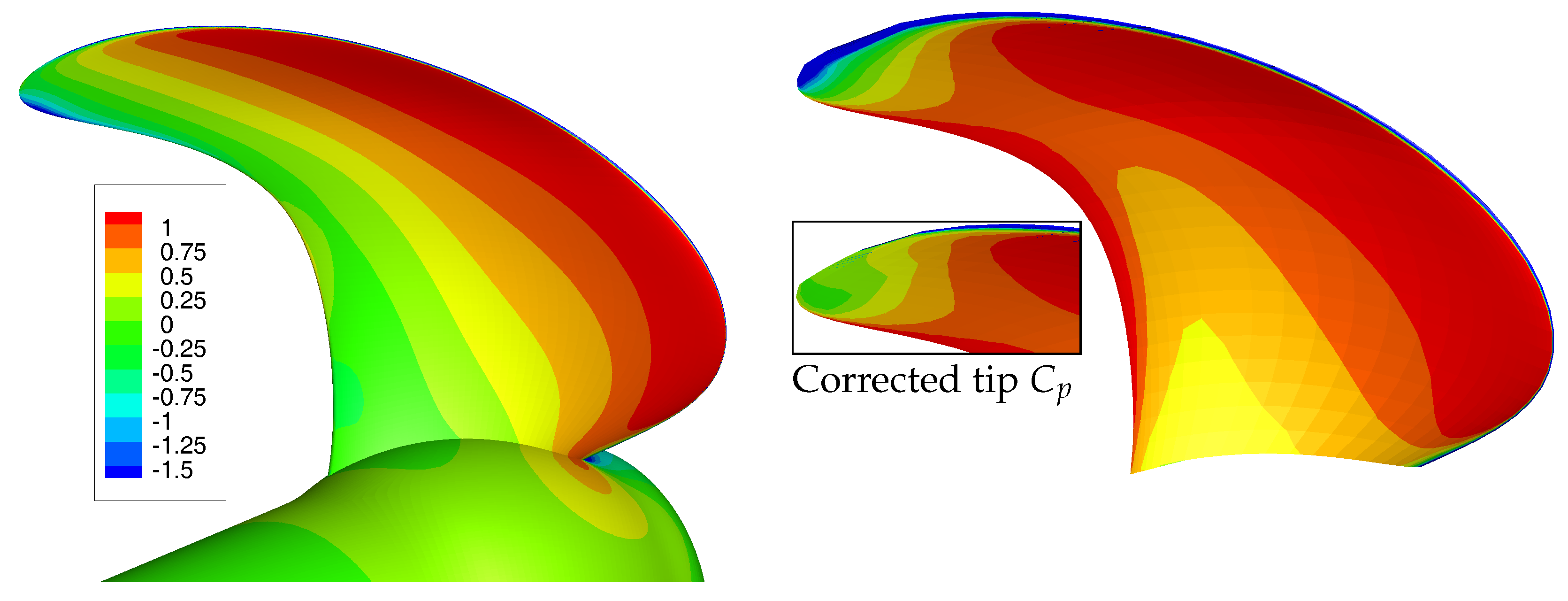
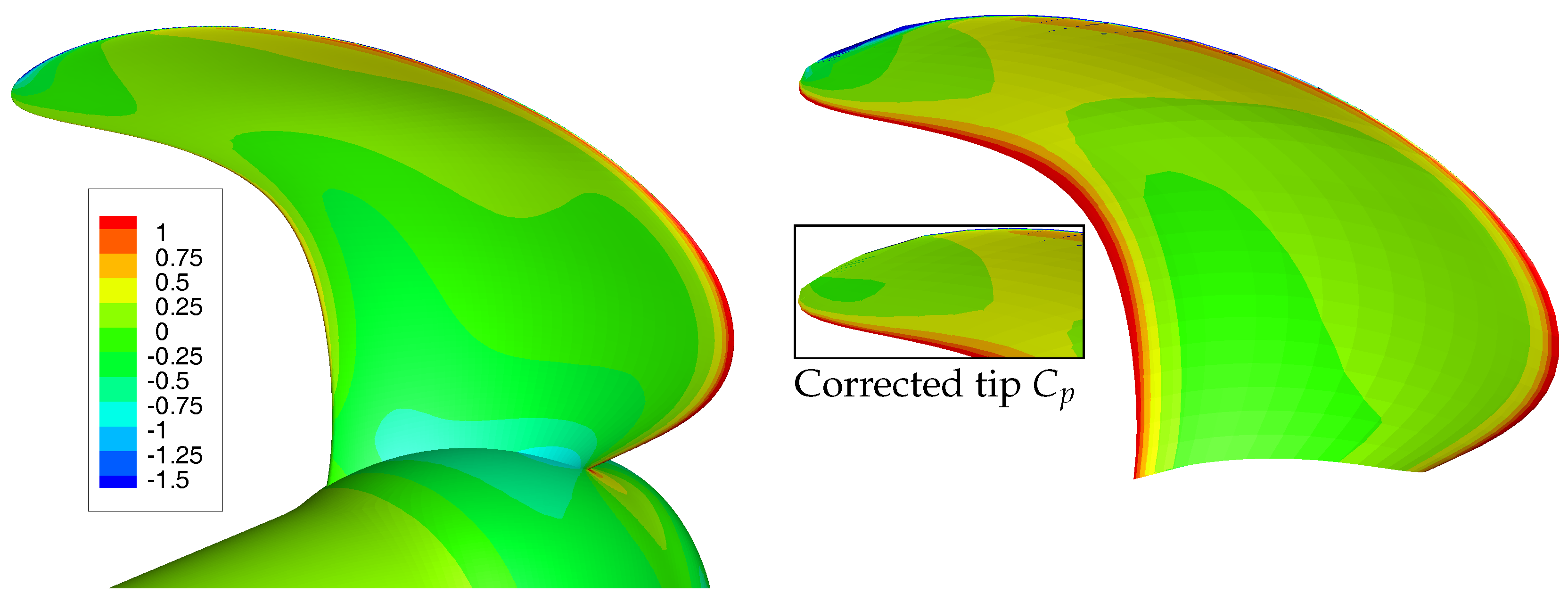
The pressure distributions for the three BEM and RANS computations are presented in Figure 7, Figure 8, Figure 9, Figure 10, Figure 11 and Figure 12. In these figures, the pressure is made dimensionless with the fluid density, propeller rotation rate and diameter. These results show that the suction side pressure is generally lower for the BEM computations. Overall, the BEM computed pressures on the pressure side are higher than those obtained from the RANS computations. These results correspond with the differences in thrust and torque between the RANS and BEM computations as presented in

Table 7. $K_T$ and $10K_Q$ for rigid propeller Reynolds-averaged-Navier–Stokes and boundary element method calculations.

	${\mathit{K}}_{\mathit{T}}$ (BEM)	${\mathit{K}}_{\mathit{T}}$ (RANS)	%	10${\mathit{K}}_{\mathit{Q}}$ (BEM)	10${\mathit{K}}_{\mathit{Q}}$ (RANS)	%
$J=0.37$	0.255	0.222	−13%	0.344	0.331	−4%
$J=0.64$	0.177	0.149	−16%	0.278	0.247	−11%
$J=0.85$	0.114	0.089	−22%	0.208	0.172	−17%

.

For the conditions $J=0.37$ and $J=0.64$, the angle of attack on the blades is high, leading to a strong suction peak in the pressure distribution. In the RANS computations, the flow separates as shown in Figure 6. At the blade tip, the differences in pressure distribution obtained from RANS and BEM computations are evident: the BEM calculations show unrealistic pressures due to a non-physical modelling of the flow. In the BEM-FEM coupled calculations, the tip pressure correction is applied to correct for that.

7. Flexible Propeller Cavitation Tunnel Experiments

Usually, thrust, torque and blade deformations are measured and used for validation of the hydro-elastic propeller calculations. In this work, the focus is on the blade deformations rather than thrust and torque values for several reasons: first of all, the deformation field provides spatially distributed information about the propeller response in contrast to the blade integrated values like thrust and torque. Secondly, the uncertainties in the measured blade deformations are smaller than the uncertainties in thrust and torque changes due to blade flexibility. The reason is that thrust and torque changes can be easily affected by unintended small deviations in propeller geometry introduced in the complicated manufacturing of flexible propellers. Stereo-photography with a Digital Image Correlation (DIC) technique was selected to measure the propeller blade deformations. With this system, a very accurate recording of the complete 3D blade deformation field was achieved.

7.1. Test Set-Up

The measurements were conducted by MARIN using their cavitation tunnel test facility. The propeller is mounted on the tunnel shaft, which is connected to an encoder. This encoder sends impulse signals used for the triggering of the strobe lights and the cameras. The test set-up used in the cavitation tunnel is explained in Figure 13. It consists of the following elements:

• Two synchronized and calibrated cameras with FireWire interface; resolution: $1388\times 1038$ pixels; maximum frame rate 16 fps at full resolution.
• Stroboscopic lights with flash duration in the micro second range. Flash duration is kept as short as possible to avoid motion blur at the blade tip.
• The shaft encoder mounted on the shaft, provides 360 pulses per revolution.
• A pulse selector is able to select one of these 360 pulses as a trigger, which is sent to the stroboscopes and the cameras. Therefore, a trigger can be supplied, with a resolution of one degree for every blade position. The cameras and the strobe are synchronized such that the strobe flash falls within the time frame that the camera shutter is open.

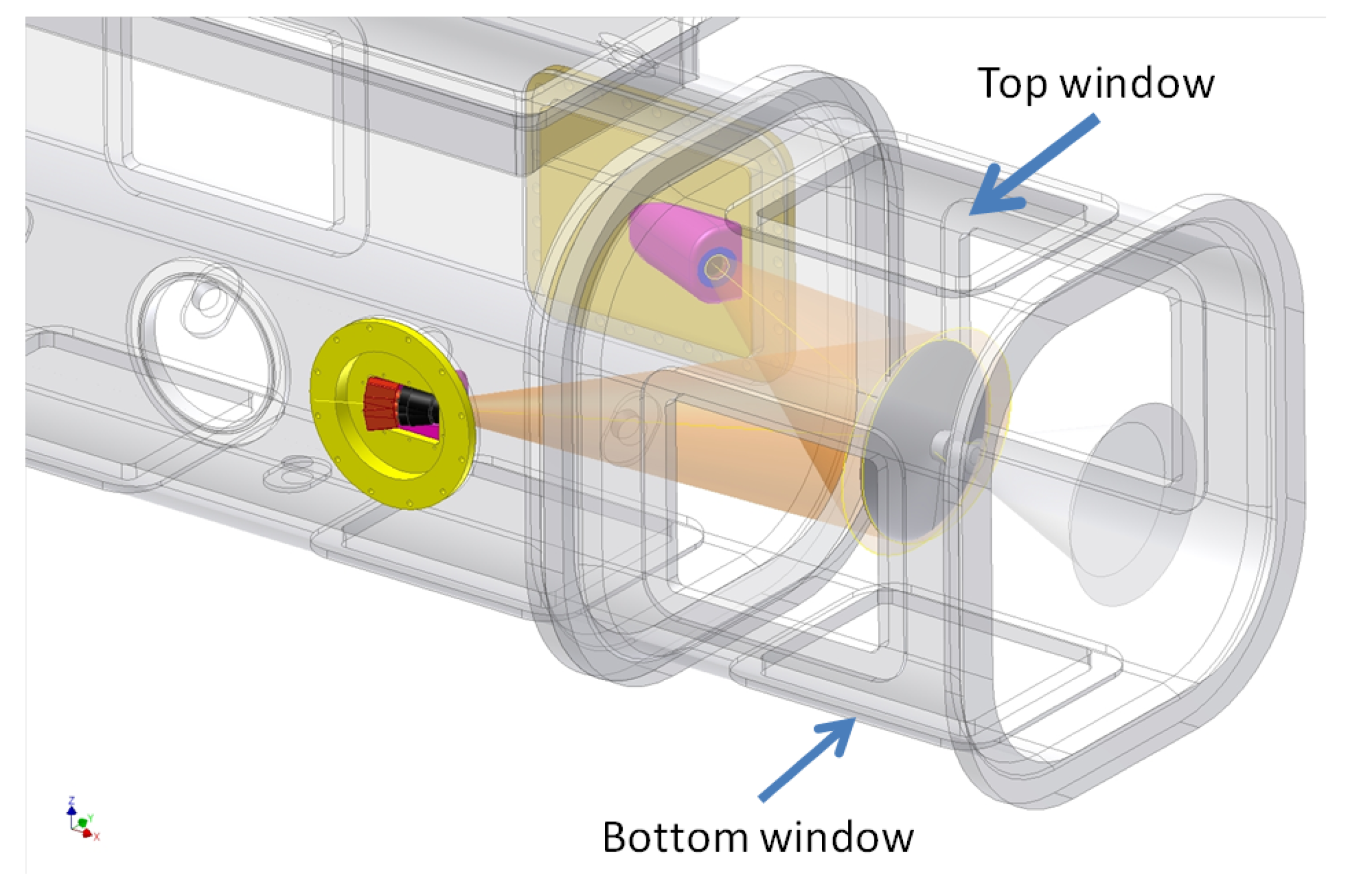
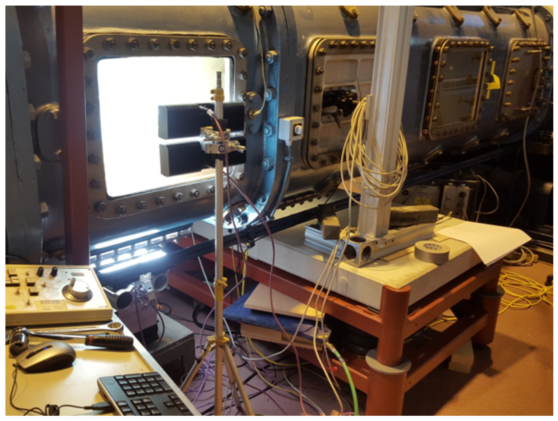
Figure 14 shows the initially proposed camera set-up. Two purpose-built windows were mounted in place of the cavitation tunnel lateral windows to have an optimal camera view. Figure 15 shows a picture of the realized test set-up. During the experiments, one of the windows was moved to the bottom of the tunnel to further improve the view on the blade surfaces. In addition, the cameras were mounted on a vibration damping structure to ensure their isolation from vibrations.

7.2. Measurement Technique

The image data acquired with the calibrated stereo camera system have been used to compute the blade deformations by means of DIC. DIC is a full-field image analysis method, based on grey value digital images, that finds the displacements and deformations of an object in three-dimensional space [33]. During the blade deformation, the method tracks the grey value pattern from which the deformations of the object are calculated. This method can be used in several applications. In particular, it has been successfully applied for blade deformation measurements both in uniform flow in the cavitation tunnel and in behind ship model condition in the towing tank [34].

In order to use the DIC technique, the surface of the measured object must have a random speckle pattern with no preferred orientation and sufficiently high contrast. The size of the features in the pattern should be large enough to be distinguished. If the material does not naturally show a usable speckle pattern, this must be applied through printing or painting. With this technique, very accurate measurements of the blade response were achieved. Several images for each blade position were acquired and image averaging was applied to filter out displacements resulting from high frequency vibrations of the propeller blade, and to remove possible bubbles or particles in the water. The results were further post-processed and a procedure was applied to correct for rigid body motions induced by vibrations and movements of the shaft.

8. Experimental, Modelling and Discretisation Uncertainties Flexible Propeller Cases

8.1. Experimental Uncertainties

Regarding the experimental uncertainties, two types of errors can be distinguished: precision errors and systematic errors. Precision errors are due to the statistical variability in the measured data set and can be reduced by repeating the test a number of times until the true average value of the measurement distribution is obtained. To reduce the precision errors in the measurements, averaging of the results was applied. Thrust, torque, flow speed and rotation rate are time averaged values. To obtain the true average displacements, image averaging with 30 images was applied. Therefore, it is expected that the precision errors are small compared to the systematic errors. Only for the DIC measurements was a precision error determined because this precision error is not reduced with the image averaging, since the results are averaged before the cross-correlation. In order to estimate this precision error, a test was performed. A rigid flat plate, with a speckle pattern, was mounted on the cavitation tunnel shaft. The displacements of the plate in the axial direction due to different tunnel speeds (from 0 to 6 m/s) were measured. Given the stiffness of the plate, bend and shear deformations of the plate can be neglected. Therefore, the measured displacements are due to the compression of the tunnel shaft and are assumed constant over the plate area. The distribution of the rigid displacement is an indicator of the precision error. A 95% confidence interval of around 20 $\mathsf{\mu }$m was obtained. From the results, it was also concluded that this precision error is independent of the displacement magnitude or tunnel flow speed (see also [23]).

A DIC systematic error of 30 $\mathsf{\mu }$m has been assumed. This value is based on the measured blade response adjacent to the hub where a zero blade displacements can be expected, but which is generally not the case. The total uncertainty for the DIC measurements becomes 50 $\mathsf{\mu }$m by simply adding the precision and systematic error together.

8.2. Modelling Uncertainties

Modelling uncertainties originate from different sources. There are modelling uncertainties due to simplifications in the mathematical models. For instance, in the BEM calculations, by assuming a potential flow and in the RANS calculations by adopting the $k-\sqrt{k}L$ turbulence model instead of a transition model, which would be able to predict the transition from laminar to turbulent flow.

There are also modelling uncertainties in the RANS-FEM and BEM-FEM calculations due to not exactly modelling the properties and conditions as appearing in the cavitation tunnel experiments. For this class of modelling errors, uncertainty levels have been estimated. The following modelling errors have been judged to be the most important, modelling errors due to:

• using the design propeller geometry instead of the as-built geometry,
• using the design propeller stiffness instead of the actual propeller stiffness,
• neglecting of the cavitation tunnel walls.

The first modelling error is due to using the design propeller stiffness instead of the actual propeller stiffness. Based on measured and computed blade natural frequencies, a stiffness systematic error of ±5% and ± 10% has been assumed for epoxy propeller and composite propellers, respectively.

An important modelling error is introduced by performing the calculations with the design geometry instead of the as-built geometry. The influence of the difference between as-built and design geometry on the blade forces was investigated by comparing results of BEM calculations obtained for the different geometries. This investigation indicated that, depending on the propeller blade and flow condition, a significant difference in thrust force due to inaccuracies in the blade geometry can be assumed (see also [23]).

The modelling error due to neglecting the tunnel walls is only relevant for the BEM-FEM calculations, since the RANS-FEM calculations were performed in a bounded circular domain. This error has been estimated with Glauert’s correction for tunnel wall effects [35]. With Glauert’s correction, the unbounded flow velocity is replaced by an equivalent mean tunnel flow speed resulting in the same thrust.

8.3. Discretisation Uncertainties

The discretisation uncertainties in the BEM-FEM calculations are smaller than 0.5% and assumed negligible compared to the modelling errors as described above. The RANS grid discretisation uncertainties in bend and twist deformations have been estimated with the same method and grids as used for the thrust and torque uncertainty estimation in Section 4.2.1. This means that, in total, twelve RANS-FEM calculations have been performed—for every flow condition, four calculations with the four RANS grids. Then, for each radial station, the uncertainties in mid-chord bend deformation and twist deformation were calculated from the solutions of the four systematically refined grids.

8.4. Total Uncertainties

Table 8. Uncertainties (lower and upper levels) in mid-chord bend deformation at the tip in (mm).

	RANS-FEM Result	Modelling Uncert. 1	Modelling Uncert. 2	Discretisation Uncert.	Total Uncert.
$J=$ 0.37	4.34	−0.157; 0.0	−0.212; 0.211	−0.386; 0.386	−0.468; 0.440
$J=$ 0.64	4.11	−0.184; 0.0	−0.200; 0.201	−0.025; 0.025	−0.273; 0.202
$J=$ 0.85	4.20	−0.233; 0.0	−0.185; 0.183	−0.290; 0.290	−0.415; 0.343

and

Table 9. Uncertainties (lower and upper levels) in twist deformation at the tip in (${}^{°}$).

	RANS-FEM Result	Modelling Uncert. 1	Modelling Uncert. 2	Discretisation Uncert.	Total Uncert.
$J=$ 0.37	−2.29	0.0; 0.066	−0.089; 0.090	−0.508; 0.508	−0.515; 0.520
$J=$ 0.64	−1.95	0.0; 0.083	−0.093; 0.091	−0.092; 0.092	−0.131; 0.154
$J=$ 0.85	−2.58	0.0;0.128	−0.101; 0.102	−0.335; 0.335	−0.350; 0.373

present the uncertainties at the propeller tip for the RANS-FEM calculations. The separate uncertainty contributions are are added in quadrature, resulting in the total uncertainties as given in the last columns. From these results, it can be concluded that the discretisation uncertainty dominates in the total bend and twist deformation uncertainty of the lowest and highest advance ratio. From this, it can be concluded that convergence of thrust and torque (as shown in Section 4.2.1) does not automatically mean that the blade structural response is converged as well.

The separate contributions of the modelling uncertainties for the composite propellers are not shown here. However, for propeller 90, the stiffness uncertainty has the largest contribution. For propeller 45, the blade geometry uncertainty has more or less the same magnitude as the stiffness uncertainty. The contribution in uncertainty due to the presence of the tunnel walls for the epoxy propeller BEM-FEM calculation was relatively large, since the stiffness uncertainty is smaller than for the composite propellers.

9. Comparison of Experimental, BEM-FEM and RANS-FEM Results

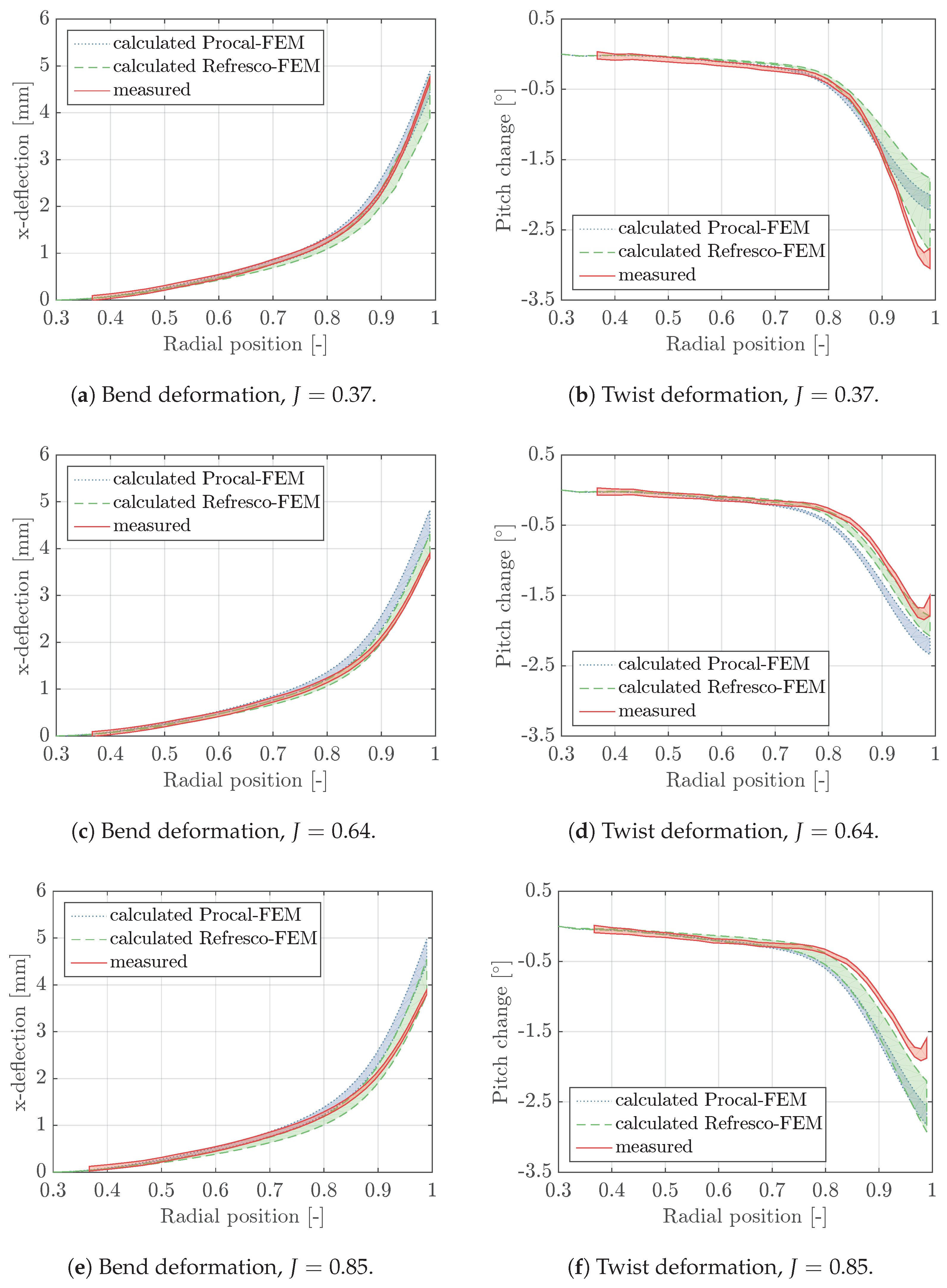
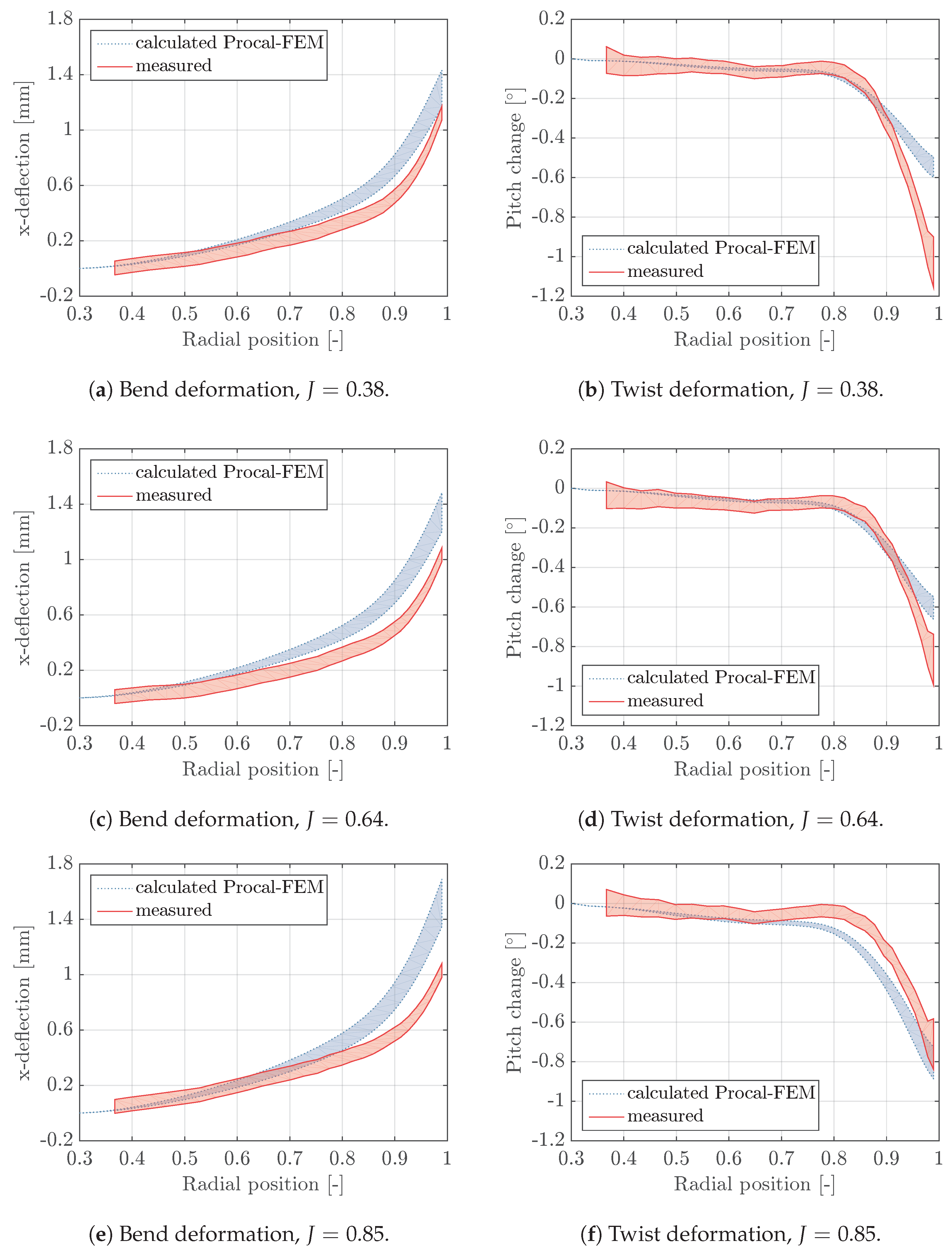
Figure 16, Figure 17 and Figure 18 show the uncertainty intervals for measured and calculated bend and twist deformations against the radial position on the blades. By investigating the results obtained for the epoxy propeller, in general, the measured bending responses are well predicted with RANS-FEM calculations. The uncertainties bandwidths for the RANS-FEM calculated twist deformations of the lowest and highest advance ratio are relatively large, mainly caused by the discretisation uncertainty, but do not partially overlap with the measurements. The differences between the twist deformations obtained from the RANS-FEM calculation and measurements for $J=0.85$ is explainable given the deviation between RANS computed thrust and the rigid propeller open water measurement as presented in Section 6.1.2 for this condition. It was pointed out that these differences might originate from modelling errors in the turbulence modelling. A plausible explanation for the differences at $J=0.37$ is the severe flow separation that might be not correctly resolved with a RANS model and the turbulence model. It can be concluded that the best agreement between measurements and the RANS-FEM calculations is obtained for the advance ratio of $J=0.64$, in which leading edge vortex separation is present but limited compared to the lowest advance ratio, and viscous forces might be less dominating than for the highest advance coefficient.

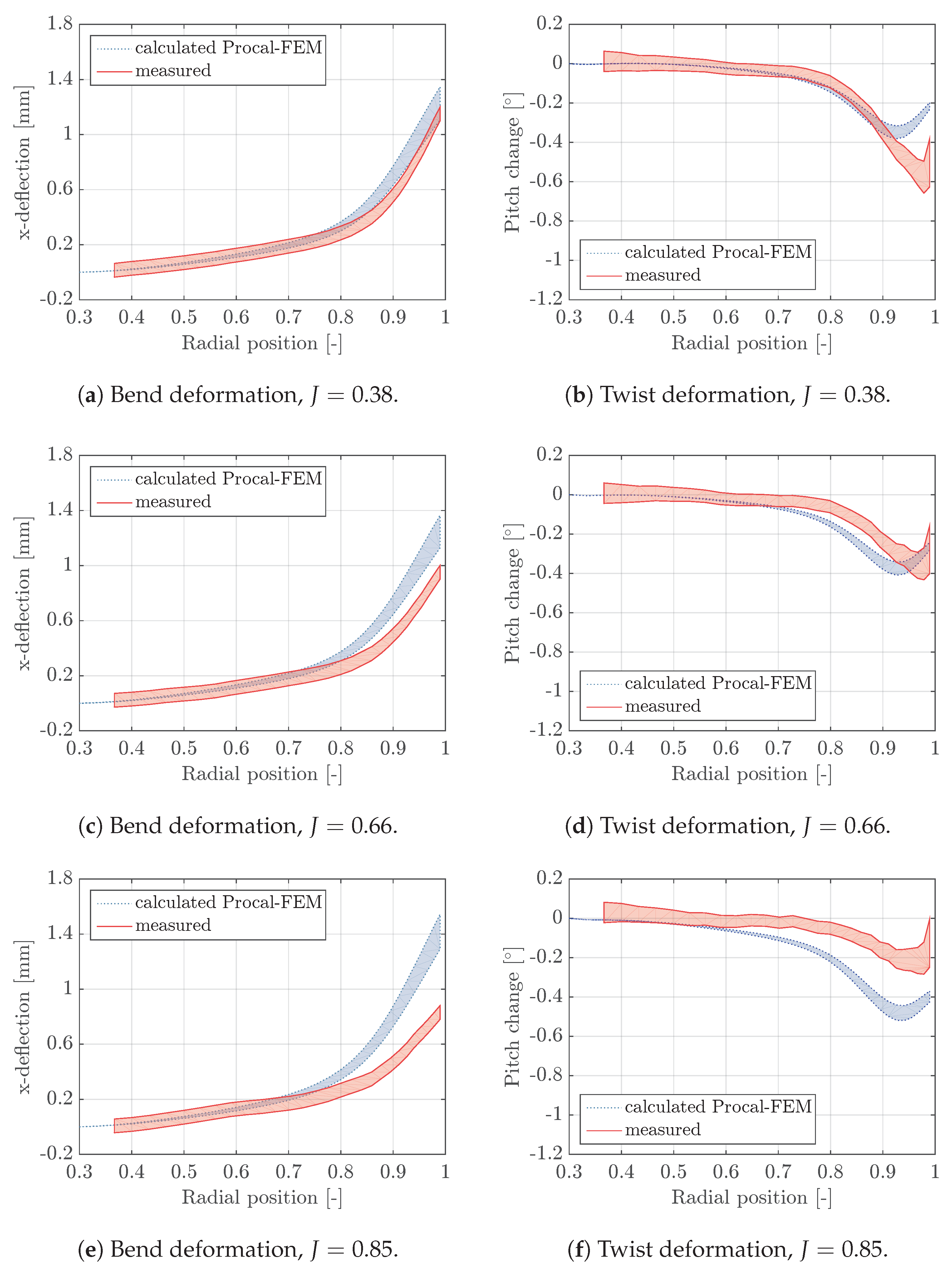
In general, the responses calculated with the BEM-FEM coupling are larger and differ more from the measured deformations than those obtained with RANS-FEM calculations. This is in line with the differences in thrust and torque computed with BEM and RANS compared to the measured open water diagram as presented in Figure 5. By looking at the BEM-FEM calculated response of the composite blades, it can be concluded that, for all the blades and loading conditions, the uncertainty intervals for measured and BEM-FEM calculated responses overlap up to 0.7 of the propeller radius. Overall, the best resemblance between measured and BEM-FEM calculated responses is obtained for the epoxy propeller. This is explained by the less complicated modelling of the epoxy material than that of composite material.

In general, the results obtained for epoxy and composite propellers are consistent: bend deformations are always over-predicted with the BEM-FEM coupling. For the twist deformations, it depends on the loading condition: for the lowest and the highest advance coefficient, the twist deformations are under-predicted and over-predicted, respectively. For the intermediate advance coefficient, the best agreement between measured and calculated twist deformations is obtained.

Since no RANS-FEM computations are performed for the composite propellers, it is difficult to examine whether the differences between calculated and measured responses for these propellers can be explained from the BEM modelling uncertainty. For propeller 45, it is assumed that this is the case, since qualitatively the predicted and measured response for this propeller is very similar to the response of the epoxy propeller. For propeller 90, the differences between measured and calculated response are larger, especially for the advance ratio of 0.85. Furthermore, the twist deformation of this propeller is completely different from the other two propellers, but qualitatively well-predicted with the BEM-FEM coupling.

10. Conclusions, Recommendations and Further Work

In this work, a BEM-FEM coupling is presented for analysing the hydro-elastic behaviour of flexible propellers in uniform flows. This code has been validated with small scale experiments and compared to the results of RANS-FEM calculations.

From the comparison between the measured open water diagram and the open water curves calculated with BEM and RANS, it can be concluded that, for the two lowest advance ratios considered in this work, the resemblance between RANS predicted and measured $K_T$ and $K_Q$ values is acceptable. The differences that were found for the highest advance ratio might originate from the turbulence modelling. A transition model might be more appropriate, especially for the highest advance coefficient, but was considered out of the current scope. It can be concluded that the open water curves calculated with PROCAL clearly show the limitations of BEM. For high advance coefficients ($J>1$), the viscous effects play an increasing role and therefore the PROCAL results become inaccurate. For $J<0.4$, a strong leading edge vortex is generated in the RANS results, and it is hypothesized that this is the reason that the results of the PROCAL calculations diverge from measured results for low advance ratios.

Interesting results are obtained from the uncertainty analysis with the RANS grids. However, the thrust and torque values were converged, and it has been shown that this does not automatically mean that the blade structural response is converged as well. Therefore, it is recommended to include a criteria on the convergence of blade bending and twisting in grid refinement studies for these types of calculations.

From the comparison of RANS-FEM and BEM-FEM results to the results of the blade deformation measurements on the epoxy propeller, it can be concluded that the bending response is well predicted with the RANS-FEM and BEM-FEM simulations. For the BEM-FEM coupling, this is despite the limitations of BEM and the complicated flow characteristics, and, therefore, it is expected that, for many other propeller geometries, the BEM-FEM coupling can correctly predict the bending response. Depending on the advance ratio, a fair to poor prediction of the twist deformations of the epoxy propeller is obtained with the RANS-FEM and BEM-FEM coupling. The best agreement between measured and calculated twist deformations is obtained for the RANS-FEM results for an advance ratio of 0.64, in which leading edge vortex separation is present but limited compared to the lowest advance ratio and viscous forces might be less dominating than for the highest advance coefficient.

The results of this work show that the differences between measured and predicted responses of the composite propellers are larger than for the epoxy propeller. This is attributed to the more complicated FEM modelling of the composite material and most likely there is a bigger spread between design and actual material properties than for the epoxy material. Therefore, it is recommended to validate these types of fluid–structure analyses with propellers made out of isotropic and flexible material. When composite materials are used, it is recommended to do the experiments on a larger scale or with very flexible composite blades so that the measurement uncertainty becomes less dominant.

Regarding the consequences of the potential flow simplifications on the FSI response of flexible propeller, it can be concluded that, for the lowest and the highest advance coefficient, the uncertainty bandwidths of the twist deformation curves obtained with BEM-FEM and RANS-FEM overlap. This is due to the large RANS-FEM discretisation uncertainty in these calculations, rather than a correct prediction of the twist deformations with the BEM-FEM coupling, since, for these conditions, the BEM-FEM predicted twist responses deviate significantly from the measurements. The differences between measured and BEM-FEM calculated twist deformations are, for the low advance ratio, explained by the strong leading edge vortex separation, which is not computed in the BEM. For the highest advance ratio, viscous effects play an increasingly important role. It is obvious that the best resemblance between measurements, RANS-FEM and BEM-FEM results, is obtained for the intermediate advance ratio for which flow separation and viscous effects play a less dominant role. Hence, it can be concluded that, with a BEM-FEM approach, the bending response can be well predicted; however, in case of extreme flow separation and viscous effects, a BEM-FEM approach for computing the twist deformations is not recommended.