Residence Time of a Highly Urbanized Estuary: Jamaica Bay, New York


1
Davidson Laboratory, Stevens Institute of Technology, Hoboken, NJ 07030, USA
2
HDR Inc., Mahwah, NJ 07495, USA
3
ARCADIS Inc., Chelmsford, MA 01824, USA
*
Author to whom correspondence should be addressed.
†
Now at the Department of Civil and Environmental Engineering, Princeton University, Princeton, NJ 08544, USA; [email protected].
J. Mar. Sci. Eng. 2018, 6(2), 44; https://doi.org/10.3390/jmse6020044
Submission received: 22 January 2018
/
Revised: 16 April 2018
/
Accepted: 17 April 2018
/
Published: 20 April 2018
(This article belongs to the Section Physical Oceanography)
Abstract
:Using a validated coupled hydrodynamic-tracer transport model, this study quantified the mean residence time in Jamaica Bay, a highly eutrophic lagoonal estuary in New York City. The Bay is a well-mixed to partially-stratified estuary with heavily-dredged bathymetry and substantial wastewater treatment plant effluent inputs that lead to seasonal hypoxia in some poorly-flushed deep-water basins. Residence time was computed for Jamaica Bay and its largest isolated deep basin, Grassy Bay. The response of residence time to freshwater discharge and wind forcing during summer 2015 was also investigated. The model results showed that the mean residence time, which represents the time required to flush out 63% of tracers released into the region of interest, was 17.9 days in Jamaica Bay and 10.7 days in Grassy Bay. The results also showed that some regions in Jamaica Bay retained their tracers much longer than the calculated residence time and, thus, are potentially prone to water quality problems. Model experiments demonstrated that summertime wind forcing caused a small increase in residence time, whereas freshwater discharge substantially reduced residence time. Freshwater inputs were shown to strongly enhance the two-layer estuarine gravitational circulation and vertical shear, which likely reduced residence time by enhancing shear dispersion. Due to the Bay’s small, highly-urbanized watershed, freshwater inputs are largely derived from the municipal water supply, which is fairly uniform year-round. This water helps to promote bay flushing, yet also carries a high nitrogen load from wastewater treatment. Lastly, the tidal prism method was used to create a simple calibrated model of residence time using the geometry of the study area and the tidal range and period.
1. Introduction
In estuaries and coastal waters, hydrodynamic processes greatly impact the transport of living biomasses, nutrients, contaminants, dissolved gasses, and suspended particles. Transport time scales, such as residence time-the time taken by a water parcel or its constituents to leave a defined region of interest through its outlets to the sea [1,2], or flushing time-a bulk or integrative parameter that describes the general exchange characteristics of a waterbody without its spatial distribution [3]-are usually used as first-order metrics of transport to assess the health and integrity of estuarine and coastal ecosystems. For example, the concept of residence time has been used to study pollutant concentrations [4], distributions of plankton [5,6], harmful algal blooms [7,8], pelagic bacteria [9], and dissolved nutrients [10,11].
Water renewal in estuaries strongly depends on environmental conditions such as tides, freshwater discharge, and wind. Water renewal due to tidal exchange is cause by asymmetries between flood and ebb flows in constricted inlets [12]. Wind influences water renewal by changing circulation patterns through local and far field effects, such as wind-induced shear stress, wind-generated waves, and Ekman transport [13]. Riverine flow influences water renewal through gravitational circulation induced by freshwater-induced baroclinic/barotropic forcing. For example, [2] showed that the residence time in Scheldt Estuary, located in Belgium and the Netherlands, is much longer in summer than in winter, mainly because of lower river discharge into the estuary during summer. Ref. [14] examined the influence of different forcing mechanisms on the residence time in Barnegat Bay, Little Egg Harbor, located in New Jersey, USA. Their results showed that meteorological events and remote coastal forcing were stronger flushing mechanisms than river discharge. They also found that about 75% of the forcing behind the residual circulation in their study area was from tides, followed by local winds (20%), rivers (5%), and remote forcing (5%). Ref. [15] showed that freshwater discharge and baroclinic forcing (i.e., density-induced circulation) affect the residence time in the Danshuei River estuarine system in northern Taiwan. They found that the residence time decreased from about 4.5 days to 2.5 days as the upstream freshwater input increased from 9 m3 s−1 to 300 m3 s−1. Their results also revealed that the baroclinic forcing significantly reduced the residence time in their study area (a reduction between about 8% and 47%, depending on the freshwater input).
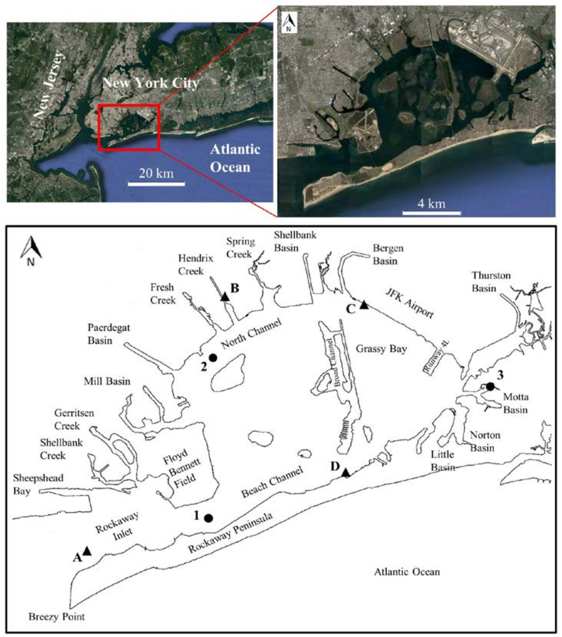
Understanding transport time scales and their response to environmental conditions can help city planners and decision makers to develop effective coastal management programs for urban estuarine systems in coastal megacities. An example of such a system is Jamaica Bay, located in the New York/New Jersey Harbor Estuary, which is one of the world’s most populated and heavily trafficked waterways (Figure 1). Jamaica Bay receives excessive nutrients, mainly from point sources including four wastewater treatment plants (WWTPs), stormwater, and combined sewer overflows (CSOs) when WWTP capacity is exceeded during heavy rain and snow storms. Due to the large nitrogen and phosphorus loading, some parts of Jamaica Bay suffer low water quality, hypoxia (low dissolved oxygen levels) and anoxia (total depletion of dissolved oxygen levels) especially during late summer. In addition to the high supply of nutrients, poor mixing and circulation in deep and stratified water bodies such as Grassy Bay provide ideal conditions for low oxygen levels in Jamaica Bay [16,17].
In the past few years, there has been strong momentum to improve our understanding of the current state of Jamaica Bay’s ecosystem and its response to environmental disturbances. A topic of interest has been the residence time in the bay and its deep-water bodies, such as Grassy Bay. There are also concerns about the effect of meteorological conditions, including freshwater discharge and wind forcing on the water circulation and residence time in the bay, owing to the fact that the forcing mechanics in the bay are subject to change under future climate conditions. Projections for the New York metropolitan region indicate large climate changes and thus the potential for large impacts [18]. Despite the importance of this research topic, the region is currently lacking information on the influence of meteorological forcing on transport time scales.
In this study, we used a three-dimensional numerical model, as well as a theoretical method to quantify the mean residence time (spatially averaged) in Jamaica Bay and its most poorly-circulated region, Grassy Bay. We first validated the model using observed water elevation, velocity, salinity, and temperature and then implemented it to quantify the residence time and its response to freshwater discharge and wind forcing. We also used the classical tidal prism theoretical method to study how the residence time may be influenced by geometry (e.g., volume of water in the system, connectivity, inlet type, etc.) and tidal range and period. This study was part of a broader project, sponsored by the U.S. National Parks Service (NPS), which aims at understanding, improving and sustaining water quality, ecosystem dynamics, hydrodynamics, and resilience to waves and flooding in Jamaica Bay. In the present study, we aimed to advance our understanding of residence time as a first-order water quality indicator in Jamaica Bay, as well as its response to freshwater discharge and wind forcing. The results of the broader project, including the results of the present study, will be used by city planners and decision makers to develop a coastal master plan for Jamaica Bay.
2. Study Area
Jamaica Bay is a saline to brackish lagoonal (or back-barrier) estuary located in the southern portion of the New York metropolitan area (Figure 1). The bay is bordered by the Rockaway Peninsula to the South, Queens to the East and North, and Brooklyn to the West, and is open to the Atlantic Ocean via Rockaway Inlet on the southwest. Tides in Jamaica Bay are predominantly semidiurnal with a mean tidal range (mean high water—mean low water) between 1.5 and 1.7 m and period of 12.42 h. Tidal forcing is the main driving force in the bay, resulting in currents up to 1.5 m s−1 in Rockaway Inlet. Water salinities in open waters typically range from approximately 20 to 26 psu and water temperatures vary seasonally from 1 °C to 26 °C [19].
Land use of Jamaica Bay’s floodplains is predominantly dense residential. Over the past 150 years, Jamaica Bay has received extensive physical alteration of its shorelines and bathymetry due to dredging, filling, and development. The average low tide depth in the bay was approximately 0.9 m prior to these changes, whereas it has increased to approximately 4.9 m today [19]. At present, Jamaica Bay consists of deep navigating channels in its perimeter and a shallower central region dominated by subtidal open water and extensive low-lying islands, including intertidal salt marshes and mudflats. The average depth of the surrounding channels is about 10 m. However, because of dredging for commercial construction and for landfilling projects in the past, some regions are much deeper than the average depth. The sand-mining operations left borrow pits-depressions on the bottom-in several locations in Jamaica Bay. For example, deep borrow pits were excavated within Norton Basin and Little Basin, two dead end basins located on the Rockaway Peninsula, during the development of the Edgemere Landfill in 1938 [20].
Grassy Bay, the deep eastern portion of Jamaica Bay, is a large single borrow pit that was dredged to construct John F. Kennedy (J.F.K.) International Airport in the 1950’s. It has a high concentration of nitrogen and low level of dissolved oxygen due to a relatively small tidal prism, poor circulation, and direct nitrogen loading from the Jamaica WWTP. Thus, vertical stratification and hypoxic conditions frequently prevail in Grassy Bay. For example, water samples collected in summer 2009 showed six hypoxia events in bottom waters, with a minimum dissolved oxygen concentration below 3.0 mg/L [16].
The primary sources of continuous freshwater flow to Jamaica Bay are the outfalls from four major WWTPs, including Coney Island, 26th Ward, Jamaica, and Rockaway, which are distributed around the perimeter of the bay (Figure 1). These WWTPs discharge about one million cubic meters of treated wastewater into the bay daily [21]. Jamaica Bay is also surrounded by many creeks and basins that receive freshwater flows only from stormwater runoff and CSOs during heavy precipitation events. The water discharges from WWTPs, stormwater, and CSOs have a significant impact on water quality and ecosystem health in Jamaica Bay. The treated wastewater from WWTPs has no pathogenic bacteria but it contains high amounts of nitrogen and other organic materials that can promote excessive algae growth, and reduce the level of dissolved oxygen, especially during warm weather. On the other hand, CSOs can contain high concentrations of suspended solids, toxic chemicals, bacteria, oxygen-demanding organic compounds, and other pollutants.
3. Methods
The residence time in estuarine and coastal systems can be measured in the field, estimated based on idealized theories, or simulated using computational models. However, residence time is rarely measured in the field because the monitoring of drifters or injected fluorescent dyes must be conducted at a large temporal and spatial scale, which makes measuring residence time difficult and expensive. In idealized systems, existing theoretical methods, such as the continuously stirred tank reactor method [3,22] and the tidal prism method [23], can be adopted to estimate the flushing time or mean residence time. Without proper calibration, these idealized theoretical methods may not provide reliable results in estuarine and coastal systems with complex geometries, and time- and space-varying driving forces (freshwater discharge, wind, tide, etc.). In such systems, numerical modeling is a relatively more cost-effective and reliable approach to determine transport time scales, such as residence time. In this study, we adopted both numerical modeling and theoretical methods to determine the mean residence time of Jamaica Bay.
Residence time is the time it takes for any water parcel to leave the system. Water parcels near the outlet have a shorter residence time than those far from the outlet, resulting in a spatially varying residence time. Moreover, physical processes that control the transport of water parcels usually vary in space (and time). The Lagrangian particle tracking model is a suitable tool to compute the spatially varying residence time (e.g., [14,15,24,25]). However, to determine the mean residence time, a particle tracking model needs to track a large number of particles, which can lead to a high computational cost, especially in a large-scale domain. The Eulerian tracer transport model, on the other hand, is a suitable tool to compute an integrative transport time scale, such as the mean residence time (e.g., [2,26,27]).
In the present study, we calculated mean residence time using an Eulerian tracer transport model, which is described in the following sub-section. The model results were analyzed to calculate the mean residence time based on the e-folding time scale [28,29]. Therefore, the mean residence time represents the time when the volumetric concentration of conservative tracers in the domain of interest decreased to 1/e (~37%) of the initial concentration in the same domain. Boundaries of the domains of interest, i.e., Jamaica Bay and Grassy Bay, are shown as dashed/dotted lines in Figure 2. We chose the boundaries of Jamaica Bay and Grassy Bay for the purpose of mean residence time computations. The entirety of Jamaica Bay is one mostly enclosed region, whereas Grassy Bay is a relatively enclosed deep area within it that is well-known to have uniquely poor flushing and hypoxia problems (e.g., [30,31]).
The boundaries of Grassy Bay simply reflect the geographical designation of this well-known poorly flushed region. Moreover, once water leaves Grassy Bay, it is mostly in two deep channels-North Channel and Beach Channel-that are relatively well-flushed and which are known to have far less of a problem with hypoxia (defined here as dissolved oxygen levels below 3 mg/L) [30,31]. The boundaries of Jamaica Bay encompass the entire study area but exclude the Rockaway Inlet which is a well-flushed system. Recall that the present study focuses on the mean residence time of Jamaica Bay which is a poorly flushed system (as a whole) compared to its inlet. Including the inlet as part of the system could lead to values of residence time that differ from those presented in the following sections, mainly because tracers that leave the inlet would dilute in NY/NJ Harbor and possibly only a small percentage of tracers would return to the system.
3.1. Three-Dimensional Tracer Simulation
3.1.1. Computational Models
In this study, we used the hydrodynamic and Eulerian tracer transport modules of Stevens Institute of Technology Estuarine and Coastal Ocean Model (sECOM) to quantify residence time and its response to freshwater discharge and wind forcing. sECOM is a variant of the Princeton Ocean Model (POM), which was originally developed by [32,33], and has been successfully applied to oceanic, coastal, and estuarine waters (e.g., [34,35,36,37,38,39,40,41,42]). sECOM is also implemented in the New York Harbor Observing and Prediction System (http://hudson.dl.stevens-tech.edu/maritimeforecast/) and the Stevens Flood Advisory System (http://hudson.dl.stevens-tech.edu/sfas/).
The hydrodynamic module of sECOM solves the three-dimensional Navier Stokes equations based on the hydrostatic pressure assumption and a mode-splitting technique [43,44]. In a Cartesian coordinate system, the continuity and momentum equations are:
where V is the flow velocity vector; u, v, and w are, respectively, the flow velocity components in longitudinal x, lateral y, and vertical z directions; ρ is the fluid density; p is the hydrostatic pressure; f is the Coriolis parameter; KM is the vertical eddy viscosity; AM is the horizontal eddy viscosity; and fveg,x and fveg,y are the vegetation-induced forces in longitudinal and lateral directions, respectively [41]. The vertical viscosities/diffusivities are determined based on the Mellor-Yamada 2.5 level turbulence closure model [45] and the horizontal viscosities/diffusivities are parameterized based on the Smagorinsky method [33,46]. Through fveg,x and fveg,y, sECOM takes into account the three-dimensional influence of wetlands on mean flow and turbulence quantities based on the vegetation-induced drag and inertia forces [41]. It also includes a robust wetting and drying algorithm for upland inundation modeling [47]. The model solves the governing equations using the finite-difference method on an Arakawa C-grid with terrain-following (sigma) vertical and orthogonal curvilinear horizontal coordinates.
The tracer transport module of sECOM solves the transport equations of the passive tracer on the same computational grid used in the hydrodynamic module. The time-dependent three-dimensional mass transport equation (with sink terms representing various loss processes) is:
where C is the tracer concentration, k is the die-off coefficient or decay rate, and AH and KH are the horizontal and vertical eddy diffusivities, respectively. The diffusivities are a fraction of the eddy viscosities (usually a fraction between 0.5 and 1). In the present study, diffusivities were assumed to be equal to eddy viscosities. The model can be applied to either a conservative or non-conservative tracer. The die-off coefficient k for a non-conservative tracer (e.g., a pathogen) is estimated using empirical formulas, whereas it is set to zero for a conservative tracer (e.g., dye). In this study, we applied the model to a conservative tracer.
The tracer transport module is one-way coupled to the hydrodynamic module of sECOM. In other words, it receives the mean flow and turbulence quantities from the hydrodynamic module in order to solve the convection and diffusion terms in the tracer transport equations. The water velocities calculated from Equations (2) and (3) are used in the convection term of the tracer transport equation, i.e., the second term on the left-hand side of Equation (5). The eddy viscosities calculated from the turbulence closure models of the hydrodynamic module are used in the diffusion terms of the tracer transport equation (the first three terms on the right-hand side of Equation (5)).
3.1.2. Computational Grid
The computational domain of Jamaica Bay, the so-called Jamaica Bay Eutrophication Model (JEM), consists of a curvilinear grid with 8740 cells and a varying horizontal resolution. The horizontal grid spacing varies between 450 m at Rockaway Inlet and 28 m at some tributary channels, such as Shellbank Basin [48]. The horizontal grid resolution is between 70 m and 150 m in most regions within the bay. The vertical grid consists of 10 terrain-following sigma layers with thin layers near the water surface and seabed, and thicker layers in the middle of the water column. The normalized thickness of the vertical layers is 0.1 on the water surface, increases to 0.15 in the middle of the water column, and decreases to 0.03 near the seabed. A higher resolution near the seabed increases the accuracy of the calculated bottom velocity and, in turn, the bed shear stress.
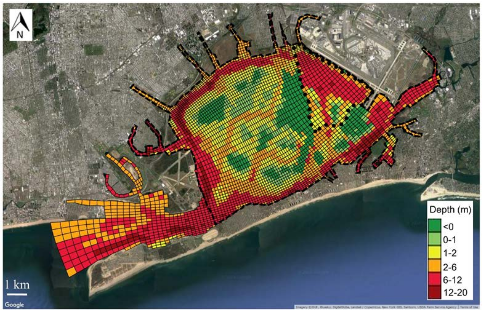
The JEM bathymetry (Figure 2) was updated for the NPS study, based primarily on topography and bathymetry data from the United States Geological Survey (USGS) Coastal National Elevation Database (CoNED) program 2014 [49], and secondarily on slightly older data collected from 2007–2008 by [50]. The LIDAR data cover dry land, marsh islands, and shallow waters and the data from [50] cover deeper waters, such as the navigating channels. The spatial distribution of salt marshes in the model is based on the New York City (NYC) urban ecological land-cover map obtained from the Natural Area Conservancy [51]. In the model, the biophysical properties of Spartina alterniflora, the dominant plant in Jamaica Bay’s salt marshes, are set to a stem height of 0.8 m, diameter of 0.6 cm, and density of 120 stems/m2 [52,53], and vegetation drag and inertia coefficients are set to the values used by [41].
3.1.3. Boundary Conditions
The model was forced with clamped elevation boundary conditions at its open boundary. The water elevation at the boundary was based on observations from the USGS site Rockaway Inlet near Floyd Bennett Field (shown as site 1 in Figure 1). Because the USGS site is located about 6 km east of the open boundary of the computational domain, we adjusted water elevations at the boundary so that a best fit between the modeled and observed water levels at Floyd Bennett Field (the location of the USGS site) was obtained. Like [41], a factor of 0.97 was applied to the observed water elevations for use as the model boundary conditions, reversing the effects of convergent topography on the tide.
The depth-dependent water temperature and salinity at the model boundary was based on a hindcast database [54] obtained from the New York Harbor Observing and Prediction System (NYHOPS). We performed a bias correction for the hindcast dataset based on the mean anomalies between the mid-depth water temperature and salinity from NYHOPS and observed mid-depth data at the USGS site Rockaway Inlet near Floyd Bennett Field. Water salinity and temperature were initialized with spatially constant values and spun-up for 30 days prior to the start date of the residence time simulations.
The atmospheric data were based on hourly observations at the Breezy Point and J.F.K. Airport weather stations. The method of [55] was used in the model to compute the heat fluxes, including shortwave solar and longwave atmospheric radiations, and sensible and latent heat fluxes. Freshwater discharge included flows from WWTPs and CSOs. Flows from WWTPs were based on measurements from the NYC Department of Environmental Protection, NYCDEP, (Bureau of Wastewater Treatment, SPDES Compliance Section, personal communication). Flows from CSOs were based on the hydrological model established by HDR Inc. for Jamaica Bay (unpublished data).
3.1.4. Mean Residence Time
The mean residence time was calculated by comparing, in each computational time step, the volumetric concentration of tracers remaining in the domain of interest with the initial concentration released in the same domain. We defined the mean residence time as the time at which the following ratio between the remaining tracer concentration and the initial concentration was satisfied:
where C(i,j,k) is the time-dependent tracer concentration at computational cell (i,j,k) with i, j, and k being the indices of coordinates; V(i,j,k) is the time-dependent volume of cell (i,j,k); the subscript zero refers to the initial value; and rmin is a constant equal to 0.37 based on the e-folding theory [3,56,57]. Per Equation (6), the mean residence time is the time that the tracer concentration remaining in the domain of interest is 37% of the initial concentration of the tracers released in the same domain. Therefore, the residence time of Grassy Bay represents the time it takes for 63% of tracers to leave Grassy Bay (its boundary is shown in Figure 2), regardless of whether they remain in other regions of Jamaica Bay or are exported to the ocean.
3.2. Theoretical Tidal Prism Method
In addition to the computational model described above, we used the classical tidal prism theory to estimate the mean residence time using tidal characteristics and the geometry of the study area. The tidal prism method relates the temporal variation of tracer concentration inside a well-mixed system to the mean residence time (or flushing time) as [3,22,58]:
where C(t) is the total concentration remaining in the system at time t, C0 is the initial concentration of tracer, and Tr,TP is the residence time. The tidal prism method determines Tr,TP as:
where V is the mean volume of water in the system, T is the tidal period, P is the tidal prism, which is the water volume between high and low tides, and b is the return flow factor that is defined as the fraction of ebb water returning to the system during the flood tide (0 < b < 1). A return flow factor of one indicates that all tracers leaving the system during the ebb tide, return to the system during the flood tide. The return flow factor is a calibrating parameter and is, importantly, a function of currents in the channel connecting the system to the open sea, as well as the amount of mixing that occurs once the water has left the system [58]. However, when there is not enough information to calibrate b, it is recommended to set b = 0.5 [58].
4. Model Validation
The tracer transport module of sECOM uses the mean flow and turbulence quantities, calculated by the hydrodynamic module, to solve the advection-diffusion equations for a passive tracer. Therefore, the reliability of the calculated residence time depends on the accuracy of the flow properties computed by the hydrodynamic module. A good agreement between the measured and calculated hydrodynamic conditions can increase confidence in the tracer transport module and its results. Therefore, to assure that the calculated residence times presented in this study were genuine, we first validated the model against the available hydrodynamic measurements in Jamaica Bay.
We compared the model results with measurements collected in July and August 2015. The calculated water elevations were compared with the measured time series from two USGS sites in the study area, i.e., Rockaway Inlet near Floyd Bennett Field and Jamaica Bay at Inwood (sites 1 and 3 in Figure 1). We also compared the calculated flow velocities with measurements collected by the Science and Resilience Institute at Jamaica Bay, and Professor Bob Chant from Rutgers University (unpublished data) at the North Channel (site 2 in Figure 1). Furthermore, the calculated water temperature and salinity were compared with measurements from USGS site Rockaway Inlet near Floyd Bennett. NYCDEP also measures water quality data, including water salinity and temperature, in Jamaica Bay. However, these measurements are spatially and temporally sparse and, thus, were not used here for model evaluation using statistical metrics (e.g., the RMSE, bias, and skill described below).
We quantified the model performance using root-mean-squared-error (RMSE), bias, and skill. RMSE was calculated as:
where X is the variable being compared, and N is the number of data points. Bias was calculated as:
and the model skill was [59,60]:
where the overbar represents time mean. Perfect agreement between the model results and measurements gives RMSE and bias values of zero and a skill of one.
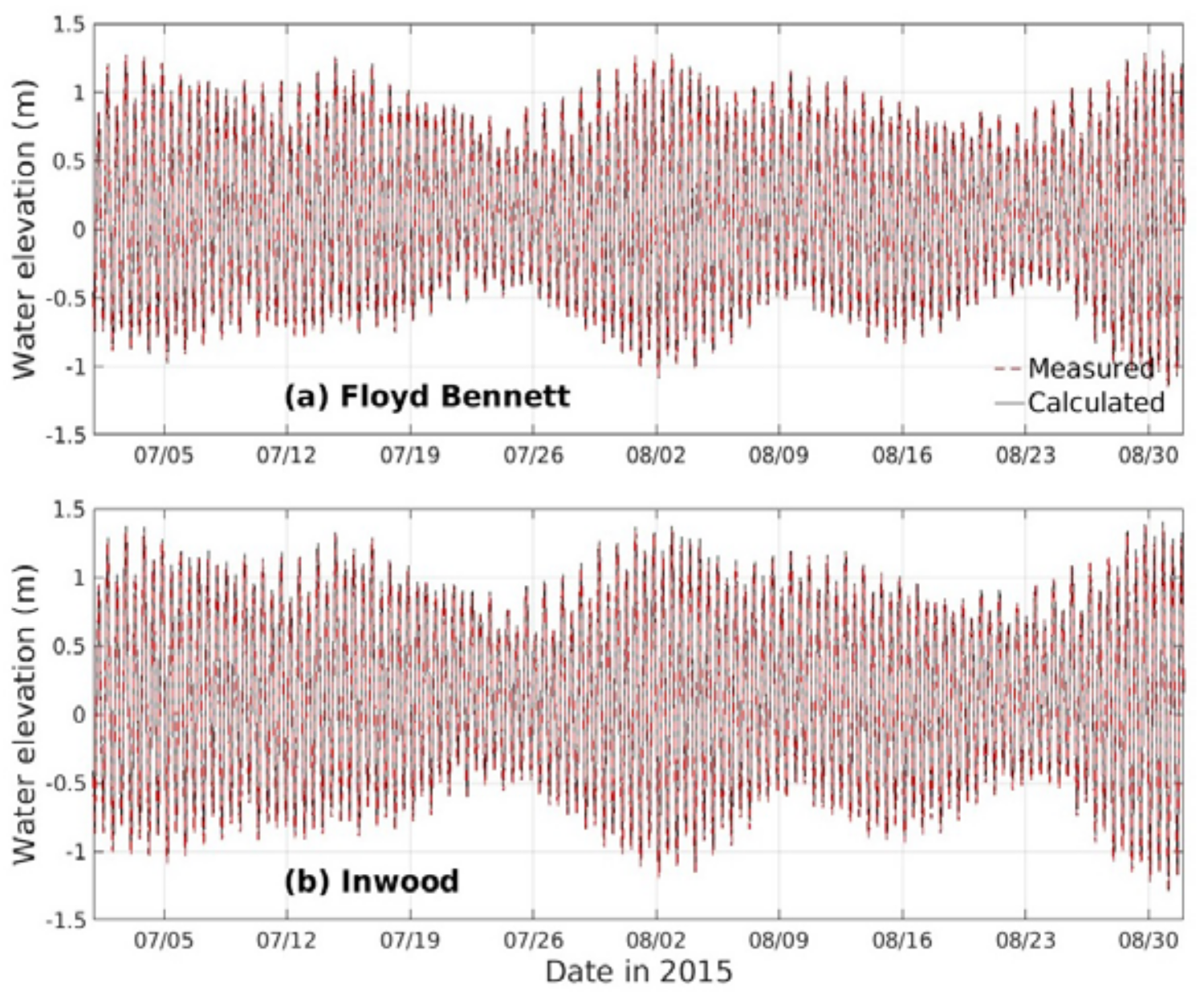
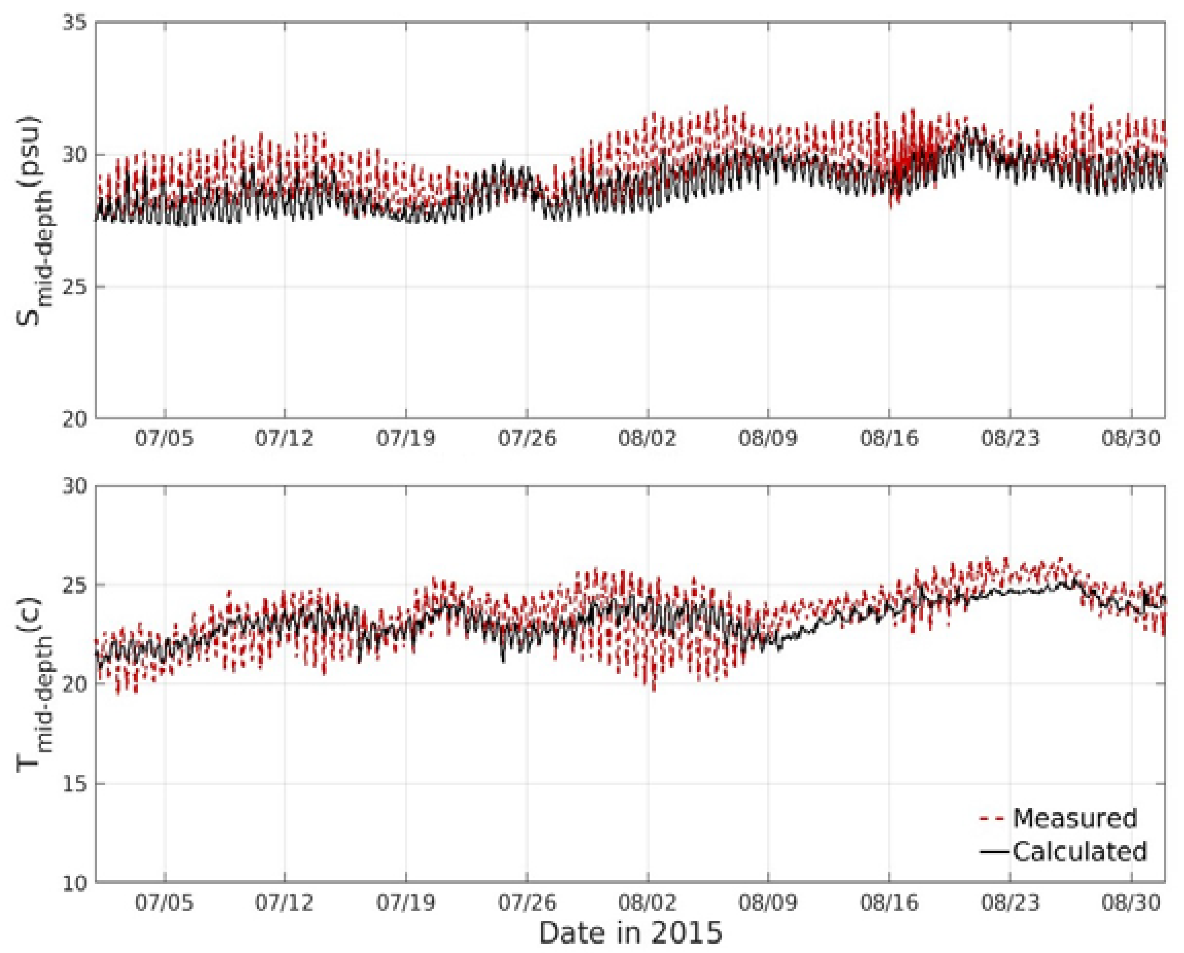
Figure 3 compares the measured and calculated times series of water surface elevation. The low RMSE and bias and excellent skill, as shown in Table 1, demonstrate the capability of the model to accurately produce the times series of water surface elevation. Figure 4 compares the measured and calculated near-surface and near-bottom velocities at North Channel. The model accurately captured tide-induced variations in the west-east and south-north components of the velocity vector. The magnitude of the velocity components were favorably reproduced with a skill of 0.93 and above (see Table 1). The modeled velocity extrema are sometimes smaller than observations, which can arise because observations are at a single point but the model grid cells reflect properties for a larger area. Finally, Figure 5 compares modeled and measured time series of water salinity and temperature. Comparisons indicate that the magnitude of the tide-induced variations was underestimated, which may be the result of errors in the model boundary conditions that were not well-constrained by salinity and temperature measurements.
Model validation was carried out based on measurements from a few locations in the study area. To better evaluate model performance, model results should have been compared with hydrodynamic measurements at more locations within the bay, e.g., at Grassy Bay and the bay’s deep tributaries, such as Thurston and Mill Basins. However, the best available field data in Jamaica Bay (for the time being) were collected at a limited number of locations (i.e., those discussed above). Collecting new field data at more locations would not only improve our understanding of the physical processes in the study area but would also provide additional measurements for model validation. For example, measuring the depth-dependent water salinity and temperature at the mouth of the Rockaway Inlet would provide accurate boundary conditions for use in the model.
5. Numerical Experiments
We implemented the validated hydrodynamic and tracer transport modules of sECOM to quantify the mean residence time during summer 2015 (between July 15 and August 25). After the model spin-up period (Section 3.1), the tracer was released in the entire water column within the domain of interest Ω (either Jamaica Bay or Grassy Bay, with boundaries shown in Figure 2), and the coupled hydrodynamic and tracer transport model was run for the next 40 days of the simulation period (i.e., between July 15 and August 25).
To evaluate the influence of different forcing mechanisms on residence time, we carried out a series of numerical experiments, as summarized in Table 2. Each experiment considered a combination of forcing mechanisms, including water elevation, freshwater discharge, and wind. Figure 6 shows the observed times series of the water elevation and the total freshwater discharge, and the wind rose diagram over the simulation period. The water elevation time series indicate spring-neap tidal cycles with no significant storm surge. The wind rose diagram illustrates that the prevailing winds were from the south, southwest, and west. The wind speed was predominantly below 6 m s−1 and rarely exceeded 9 m s−1. The time series of freshwater discharge showed a continuous constant discharge of about 10 m3 s−1 from WWTPs over the entire simulation period. The time series also showed intermittent CSOs during three rainfall events on July 30, August 11, and August 21 with maximum intensities of 12.7, 15.5, and 45.4 mm per hour, respectively (according to recorded data from the J.F.K. Airport weather station). The total rainfall in July and August 2015 was, respectively, 5.9 cm and 9.2 cm, close to (24% below) the climatological average conditions for the station.
To consider the influence of the timing of tracer release in the domain, each experiment was run for two different tracer release timings: at high tide and low tide. The release timings at high and low tide represent, respectively, the time of high and low water levels in Jamaica Bay’s inlet (i.e., at the USGS site Rockaway Inlet near Floyd Bennett Field). Separate tracer experiments were also carried out for Jamaica Bay and Grassy Bay. Therefore, in total, we performed 16 different numerical experiments.
6. Results and Discussion
6.1. Mean Residence Time in the Study Area
Table 3 shows the calculated mean residence time for each numerical experiment described above. The model with all forcing mechanisms (ALL) computed a residence time of 17.94 days for Jamaica Bay and 10.65 days for Grassy Bay. We also calculated (not shown in Table 3) the residence time of Jamaica Bay when tracers were released only in Grassy Bay instead of the entire bay. In this case, the residence time of Jamaica Bay was 22.61 days, which was 4.67 days longer than when tracers were released in the entire system.
In all experiments, releasing the tracers at the time of the low tide resulted in a longer residence time. When the tracers for a given region (e.g., Grassy Bay) were released at low tide, the incoming flood tide pushed the tracers near the region’s boundaries further into the region. Therefore, the tracers accumulated far from the outlets, and consequently they required a slightly longer time to leave the region through its boundaries. When the tracers were released at the high tide, on the other hand, the tracers near the boundaries were carried outside the region by the first ebb tide, resulting in a shorter residence time. Other studies have also shown that transport time scales strongly depend on the timing of tracer release (e.g., [2,61]). For instance, [2] used a depth-averaged hydrodynamic-tracer transport model to compute the average residence times of 13 subdomains in Scheldt Estuary, located in Belgium and the Netherlands. In all subdomains, they found that the model with tracers released at a low tide computed a longer residence time compared to the model with tracers released at a high tide.
6.2. Influence of Wind and Freshwater Discharge
Forcing from wind and freshwater discharge is summarized in Figure 6, as presented in Section 5. The wind forcing during the simulation period was induced by winds with speeds of up to 9 m s−1, predominantly from the south, southwest, and west. The freshwater forcing was associated with constant discharge from WWTPs and intermittent CSOs during three rainfall events. The model results for July 15 to 25 August 2015 showed that Jamaica Bay’s deep channels (e.g., North Channel and Beach Chanel) varied from well-mixed to partially-stratified estuarine conditions. During and after spring tides, the vertical (top-to-bottom) density differences were smaller than 1 kg m−3, and after the neap tide, the density differences were up to 2 kg m−3 (differences over a 10 m water column). Density differences were predominantly driven by salinity, except in stagnant areas of the bay, such as Grassy Bay, where the differences in summer are occasionally driven equally by saline and thermal stratification.
The results shown in Table 3 indicate that excluding the wind forcing (model NW) caused a slight reduction in the calculated mean residence times. The contribution of wind forcing to the residence time in Jamaica Bay and Grassy Bay increased to 6% and 2%, respectively. The subtle influence of the wind forcing on residence time could be due to the low speed of prevailing winds during the simulation period. Winds were occasionally above 6 m s−1 and winds of this magnitude could impact the flushing of shallow regions, such as the central area of Jamaica Bay where the water depth changes between tens of centimeters to about 2 m. However, most the tracer mass was in deep areas, as the bay’s average depth is about 5 m. In these areas, except for a thin layer near the water surface, the influence of wind-induced shear stress on transport processes during the simulation period was of secondary importance. To better evaluate the impact of wind forcing on the residence time in Jamaica Bay, we ran the model ALL with idealized wind scenarios, i.e., westerly and easterly winds with a constant speed of 6 m s−1. The calculated residence time for the idealized wind forcing was about 11% larger than the residence time from the model NW (no wind forcing). We also ran the model for a higher constant wind speed (10 m s−1) and found that, regardless of the direction of the winds (westerly or easterly), stronger winds further increased the residence time in Jamaica Bay (an increase of about 14%).
The wind-induced increase in the mean residence time can be related to the impacts of wind forcing on physical transport processes. Depending on the wind speed, duration, and fetch, the momentum transfer from the wind to the water column can influence transport processes, such as advection and diffusion, and vertical mixing and circulation. For example, using a 3-D hydrodynamic model, [62] showed that up- and down-estuary winds can reduce stratification in Chesapeake Bay. Based on observations from the York River Estuary, [63] found that wind forcing can impact the vertical shear and, thus, can either increase or decrease vertical stratification. For high-speed wind events, local surface waves (and swells) can further influence transport processes through wave-current interactions (e.g., as seen by [64]), wave-generated turbulence, orbital velocity, and momentum transfer from breaking waves to the mean flow. Jamaica Bay is a back-barrier coastal system and is sheltered from ocean swells by the Rockaway Peninsula. However, local waves generated by high-speed winds, especially during winter storms, could influence the water circulation of the bay. No study has yet been devoted to the wind and wave effects on the physical processes in Jamaica Bay. A comprehensive estuarine circulation study would improve our understanding of the important physical processes in Jamaica Bay that are influenced by wind forcing.
The model results in Table 3 show that excluding freshwater discharge (model NF) caused a substantial increase in calculated mean residence times. In Jamaica Bay, the model with all forcing (ALL) computed a residence time of 17.94 days, whereas the residence time calculated by the model neglecting freshwater discharge (NF) was 22.61 days. In Grassy Bay, excluding freshwater discharge increased the residence time from 10.65 days to 13.02 days. Therefore, the influence of freshwater discharge on residence time during the simulation period was to reduce it 21% in Jamaica Bay and 18% in Grassy Bay.
The reduction in mean residence time caused by freshwater discharge may have been due to changes in the baroclinic flow, barotropic flow, vertical mixing, or circulation. To better evaluate the influence of freshwater discharge on residence time, we compared the vertical profiles of the calculated time-averaged velocity in the presence and absence of freshwater discharge. The time-averaged velocity was defined as the velocity averaged over the first 30 days of the residence time simulation period. Note that the majority of the tracers left Jamaica Bay in the first 30 days. Figure 7 shows the vertical profiles of the time-averaged velocity at two sites: one at North Channel (lat = 40.627, lon = −73.882, depth = 11 m), which is the deep channel on the northern side of the bay, and the other at Beach Channel (lat=40.584, lon = −73.836, depth = 12 m), which is the bay’s southern deep channel. Velocities were rotated into their principle axes-the angle of maximum variance of the flow-to determine streamwise and transverse components of the velocity field. At the site located at North Channel, the streamwise up-estuary flow direction was 37 degrees counterclockwise from east (positive/negative flows indicate approximately northeastward/southwestward flows). At the site at Beach Channel, the streamwise up-estuary flow direction was 12 degrees counterclockwise from east (positive/negative flows indicate approximately eastward/westward flows). Figure 7 indicates that the freshwater discharge importantly influenced the streamwise velocities in both the northern and southern deep channels. Freshwater inputs strongly enhanced the two-layer estuarine gravitational circulation and vertical shear, enhancing shear dispersion and giving a likely explanation for the reduction in residence time (e.g., [65]). Vertical profiles of time-averaged velocities over the channel banks, not shown here, also indicate that freshwater inputs strengthened residual circulation.
Freshwater discharge during the simulation period was mainly from WWTPs, which provided a background freshwater flow of 10 m3 s−1 and 84% of total freshwater discharge during the period. This is because Jamaica Bay has a very small watershed, only a few times larger than the bay itself, and about 2 million residents and their associated municipal water use [19]. This water helps to promote bay flushing, yet also carries a high nitrogen load from wastewater treatment. Three rainfall events generated excessive CSOs and abrupt spikes in the total amount of freshwater inflow to the system (Figure 6b). The largest inflow occurred 35 days after the tracers were released into the system (i.e., August 21), during a storm event with a total daily rainfall of 6.3 cm. On the other hand, the model results showed that the residence time in Jamaica Bay was 17.94 days. Therefore, the intense rainfall event of August 21st did not overlap with the period of the calculated residence time. To better evaluate the impact of an intense rainfall event on the residence time, we performed a freshwater timing sensitivity experiment by running the model (ALL) for a scenario where the rainfall event of August 21st occurred on July 17, i.e., two days after the tracers were released in the domain. We used “model ALLfts” to refer to this freshwater timing sensitivity experiment. Table 4 shows the calculated residence times from model ALLfts and compares them with the results from model ALL. The comparisons show that the early occurrence of excessive CSO on August 21st changed the residence time in Jamaica Bay from 17.94 days to 16.89 days, a reduction of about 6%. The residence time in Grassy Bay was reduced from 10.65 to 10.15 days, about 5%. The results presented here show only a minor importance of the timing of rainfall events, suggesting that the system may have a relatively uniform residence time year-round.
6.3. Spatial Distribution of Tracer Concentration
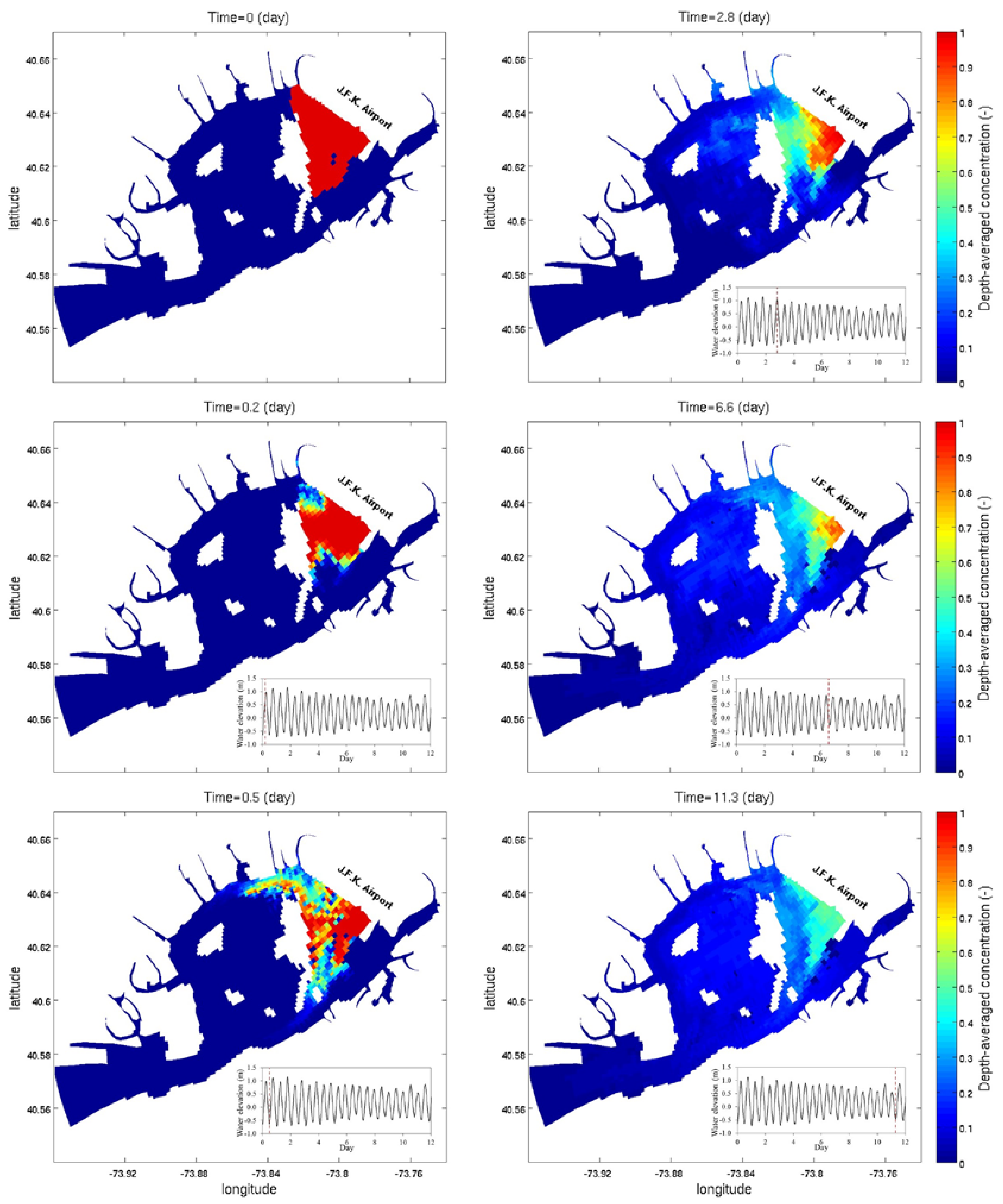
We also investigated the spatial distribution of tracer concentration in the study area. Figure 8 shows snapshots of tracer concentration for a case where the tracers were released in Grassy Bay. During flood tides, e.g., the snapshot at time = 0.2 day, the tracers were pushed farther into Grassy Bay, whereas during ebb tides, e.g., the snapshot at time = 0.5 day, the tracers were transported outside the domain. The tracer concentration near the extension of J.F.K. airport’s runway 4L remained higher than the concentration in other regions. For example, after 11.3 days, the concentration in this part of Grassy Bay was still above 0.5, whereas the concentration in other regions was below 0.3. The model results also revealed the existence of a transport pathway along Broad Channel on the western side of Grassy Bay. The tracers within this pathway left Grassy Bay throughout its northwestern and southern outlets within a relatively short time. The tracers that left Grassy Bay were first transported to the shallow regions in the center of Jamaica Bay (day 2.8) and were later dispersed very broadly towards the Rockaway Inlet (day 6.6).
As illustrated in Figure 8, the eastern part of Grassy Bay near the extension of J.F.K. airport’s runway 4 L retained the tracers much longer than other regions. Therefore, this region could have the highest mean biological oxygen demand and concentration of nitrogen and phosphorus, the lowest amount of dissolved oxygen and diversity of species, and the largest percent of clay on the bottom sediment. Moreover, the mean residence time of Grassy Bay certainly underestimates the retention time of tracers in this poorly-circulated, nearly stagnant region.
Figure 9 shows snapshots of the spatial distribution of tracer concentration for the case where the tracers were released into Jamaica Bay. The snapshots at time = 17.3 and 24.8 days recap the long-term retention of tracers near the extension of J.F.K. airport’s runway 4L. Moreover, the arms (tributaries) of Jamaica Bay retained the tracers longer than the bay’s central region and the deep channels in the perimeter of the bay. For example, after 24.8 days, the tracer concentration in Shellbank Basin, Thurston Basin, Motts Basin, and Norton Basin was still above 0.6, whereas the concentration in the center of the bay was below 0.3. Therefore, the mean residence time of Jamaica Bay should not be used as a transport time scale in these poorly-circulated parts of the bay. Separate simulations should be carried out to determine space-dependent residence times in Jamaica Bay. A Lagrangian particle tracking model (e.g., [14]), even though it can be computationally expensive, would provide more information about the spatially varying residence time in Jamaica Bay.
6.4. Results from Tidal Prism Method
To estimate the mean residence time using the tidal prism method, we first determined the surface area and average volume of water in the study area. The computational grid of Jamaica Bay (JEM grid) indicates that the surface area and volume of water are, respectively, about 5.52 × 10⁷ m2 and 24.71 × 10⁷ m3 in Jamaica Bay (excluding its inlet), and about 0.86 × 10⁷ m2 and 4.84 × 10⁷ m3 in Grassy Bay. We used an average tidal range of 1.6 m (averaged between neap and spring tides) to calculate the tidal prism. The results of our tide modeling, not shown here, revealed that the tidal range is between about 1.57 m and 1.65 m in the study area, including Grassy Bay. Using the water surface area and the average tidal range, the tidal prism was approximated to be 8.84 × 10⁷ m3 for Jamaica Bay and 1.38 × 10⁷ m3 for Grassy Bay. By setting the return flow factor, b, to a default value of 0.5 and the tidal period to 12.4 h, the calculated residence time was 2.89 days for Jamaica Bay and 3.64 days for Grassy Bay, which were significantly smaller than the values calculated by sECOM (17.94 and 10.65 days). The tidal prism method calculated a larger residence time for Grassy Bay than Jamaica Bay. This was because of the larger ratio between the mean volume of water and the tidal prism (V/P, see Equation (8)) in Grassy Bay.
The remarkable difference between the calculated mean residence times based on the numerical model sECOM and the tidal prism theoretical method might be due to the assumptions used in the theoretical method, e.g., the assumption of a well-mixed tidal system. However, the major cause of such large discrepancies may be due to an inappropriate return flow factor used in the tidal prism method, as previous studies have shown that the prediction of tidal flushing is quite sensitive to this factor. For example, [58] applied the tidal prism method to the Bay Colony Marina in Indian River Bay, DE, and found that a recommended return flow factor of 0.5 caused significant errors in the calculated residence time. Using measurements of dilution of the plume of dye, they calibrated the return flow factor and found that it greatly deviated from the recommended value. Herein, using the model results presented in the previous section, we carried out a calibration process to determine the return flow factor, b, of the tidal prism method for Jamaica Bay and Grassy Bay.
To calibrate b, we replaced Tr,TP in Equation (7) with the mean residence time calculated by sECOM (i.e., the values in Table 3) and back calculated the return flow factor. Table 5 shows the calibrated b for each numerical experiment tested in the previous section. In Jamaica Bay, the calibrated b ranged from 0.90 to 0.95, whereas it ranged from 0.81 to 0.88 in Grassy Bay. Larger return flow factors in Jamaica Bay may be due to the different hydrodynamic characteristics of different regions in the study area. Ref. [58] identified that “the phase of tidal flow in the connecting channel relative to the flow along the coast, the strength of the channel flow relative to the strength of the coastal flow, and the amount of mixing that occurs once the basin water has been ejected into coastal waters” significantly impact the return flow factor. The outlets of Jamaica Bay and Grassy Bay are located in regions with different hydrodynamic properties, which greatly affects the fraction of tracers returning to the system during flood tides. While the outlet of Jamaica Bay is bordered with the Rockaway Inlet, a deep 7 km-long channel with strong currents, Grassy Bay’s outlets are located near shallow wide areas dominated by wetlands and weak currents.
The large return flow factor in Jamaica Bay may be also due to the effect of the inlet, which was not included in the control volume that represents Jamaica Bay. Tracers that leave the bay remain in the inlet during a few tidal cycles before entering the ocean. We did not include the inlet as part of the control volume because the presence of strong currents in the inlet leads to a well-circulated system compared to the bay, which suffers poor circulation and issues related to water quality.
To cross check the calibrated return flow factors, we used the time series of tracer concentration calculated by the numerical model to estimate the percentage of tracers that returned to the system during flood tides. We calculated the return flow factor by comparing the amount of tracers that left the domain of interest during the ebb tide with the amount of tracers that entered the domain during the successive flood tide. The amount of tracers that left the domain during the ebb tide was calculated by subtracting the total volumetric concentration of tracers at the time of low tide (i.e., when the tidal level in the outlet of Jamaica Bay was at low tide) from that at the time of the preceding high tide. The amount of tracers that entered the domain during the flood tide was calculated by subtracting the total concentration of tracers at the time of low tide from that at the time of the successive high tide. The results from the model ALL showed that between 75% and 100% (with an average of 85%) of tracers that left Jamaica Bay during ebb tides returned to the system during flood tides, which satisfactorily agrees with the return flow factors calibrated for the tidal prism method.
Previous studies have used widely different values for the return flow factor b. For example, ref. [66] set b equal to 0.3 to determine the flushing time in a large number of marinas along the Spanish coast, whereas [67] set b to 0.7 for Mundaú Lagoon in Brazil. The small value of b used by [66] may be due to the fact that most coastal systems along the Spanish coast are coastal systems open to the sea and, thus, tracers that leave the system immediately are diluted into the sea and only a small portion of tracers return to the system. Ref. [67] found that the tidal prism method (with b = 0.7) significantly underestimated the flushing time of Mundaú Lagoon. While their numerical simulation based on the e-folding theory calculated a flushing time on the order of months, the tidal prism method calculated a flushing time on the order of days. They adopted the return flow factor of 0.7 based on salinity data analysis in Mundaú Lagoon carried out by [68], who specified that only 30% of the flood flow contained new water from the ocean. Ref. [67] used a control region that excluded the long, narrow inlet of Mundaú Lagoon. A return flow factor larger than 0.7 could take into account the effect of returning flows from the inlet to the control region and consequently result in a flushing time which is at the same order of magnitude as the flushing time calculated by the numerical model. For example, using the information about tides and water volume in Mundaú Lagoon provided by [67] and adopting a return flow factor of 0.95, the calculated flushing time would be on the same order of magnitude as the flushing time calculated by the e-folding method for Mundaú Lagoon.
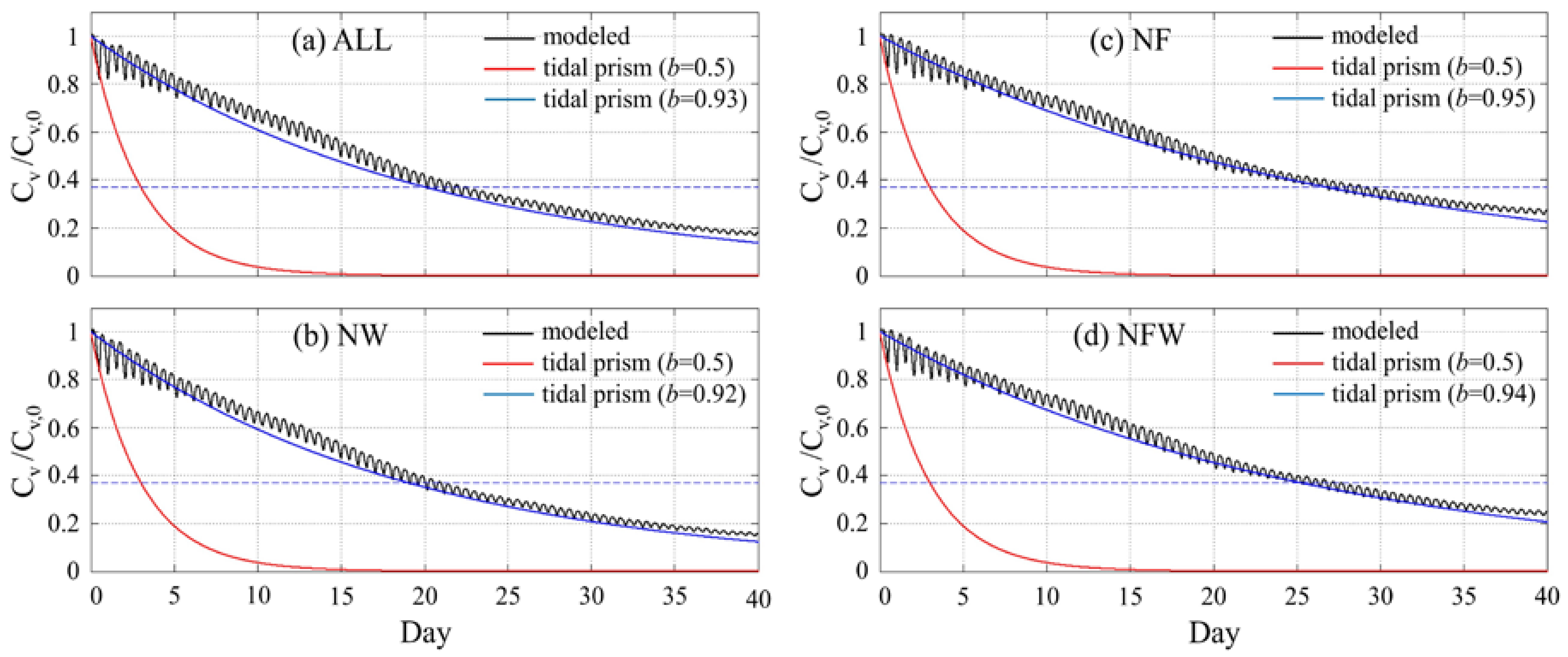
By knowing the flow return factor b in our study area, we could use the tidal prism method (Equation (7)) to generate a time series of the total tracer concentration in the study area. Figure 10 compares the time series of the tracer concentration calculated by the tidal prism method and sECOM. While the calculated time series from the tidal prism method with b = 0.5 considerably mismatched the modeled time series from sECOM, the time series produced based on a calibrated b were in good agreement with those from sECOM. Figure 10 shows that a return flow factor of 0.5 caused the tidal prism method to significantly overestimate the tracer concentration decay in Jamaica Bay. On the other hand, the tidal prism method based on a calibrated b accurately duplicated the temporal variations in tracer concentration. The time series from sECOM showed profound tide-induced variations in tracer concentration, especially during the first few days of the simulation period, which cannot be captured using the tidal prism method. In each tidal cycle, ebb tides carried the tracers near the domain outlet to Rockaway Inlet, whereas flood tides returned the tracers back into the domain. The impact of tidal cycles gradually diminished as the tracer concentration in Jamaica Bay decreased over time. The time series also revealed that at the end of the simulation, between 16% and 25% of the released tracers remained within Jamaica Bay. The largest portion of unflushed tracers remained in the east and southeast of the bay, i.e., in Grassy Bay, Thurston Basin, Motta Basin, and Morton Basin.
7. Conclusions
Using the coupled three-dimensional hydrodynamic and tracer transport modules of sECOM, we quantified the mean residence time in Jamaica Bay, New York, and its deepest portion, Grassy Bay. We first validated the hydrodynamic model by comparing measured and calculated water elevation, velocity, temperature, and salinity. The validated model was then implemented to quantify the residence time and its response to freshwater discharge and wind forcing during summer 2015. We also used the classical tidal prism theoretical method to estimate the residence time using basic information, such as the geometry of the study area, and the tidal range and period.
Based on the model application of a 40-day simulation period in July and August 2015, the model results showed that the mean residence time was 17.94 days in Jamaica Bay and 10.65 days in Grassy Bay. We found that the influence of freshwater discharge, which is mainly from WWTPs, on residence time was to reduce it 21% in Jamaica Bay and 18% in Grassy Bay. The numerical experiments indicated that an intense rainfall event might only slightly improve flushing the tracers out of the system and, thus, reduce the residence time. The present study also showed that wind forcing caused a 6% and 2% increase in residence time, respectively, in Jamaica Bay and Grassy Bay. Using idealized wind forcing experiments (with constant westerly and easterly winds), we found that the residence time in Jamaica Bay was less sensitive to wind direction but more sensitive to wind speed. The faster the wind, the longer the residence time.
The spatial distribution of tracer concentration showed that some regions in the study area, such as the eastern part of Grassy Bay near the J.F.K. airport’s runway 4 L, Shellbank Basin, Thurston Basin, Motts Basin, and Norton Basin, retained tracers much longer than other regions. This longer retention time may be due to the weak currents and poor circulation in these regions. The residence times of these poorly-circulated regions are, thus, longer than the mean residence times of the whole system presented in this study. Additional studies are needed to determine space-dependent residence times in these subdomains.
The application of the tidal prism method to Jamaica Bay showed that residence time was sensitive to the flow return factor b. By using the results from sECOM, we carried out a calibration process and found that the average return flow factor was 0.92 in Jamaica Bay and 0.83 in Grassy Bay. The time series of the tracer concentration showed that while the tidal prism method, with a default return flow factor of 0.5, incorrectly calculated the exponential decay of the tracer concentration, it accurately reproduced the concentration decay when b was set to the calibrated values. Therefore, using the tidal prism method and the suggested return flow factors in the present study, it may be possible to determine a first-order estimate of the mean residence time and the tracer concentration decay in Jamaica Bay.
As a final remark, the present study demonstrated how a highly urbanized lagoonal estuary responds to freshwater and wind forcing, as well as how this response can be relatively insensitive to moderate variations driven by weather events. The bay’s freshwater inputs are relatively constant compared with most estuaries, due to the dominance of the municipal water discharge. The deep-dredged channels and 5 m average depth of the bay render its flushing relatively insensitive to directional or normal day-to-day speed variations in winds. These results suggest that the bay’s flushing is more strongly controlled by human decisions than by environmental factors. This raises the possibility that the bay’s flushing will be relatively insensitive to variations in the wind patterns, temperatures and precipitation induced by future climate change. In ongoing work, we are evaluating the more complicated effects of climate change and coastal adaptation on flooding using an over-land flood model and hypoxia using a detailed biogeochemical model.
Acknowledgments
This research was funded by the United States Department of the Interior and National Parks Service (cooperative agreement number: P14AC01472) and National Oceanic and Atmospheric Administration’s Coastal and Ocean Climate Applications program award NA160AR4310157. We would like to thank Bob Chant from Rutgers University for sharing the hydrodynamic measurements in Jamaica Bay. We also thank Nickolas Kim from HDR Inc. for his contribution to the development of Jamaica Bay’s computational grid.
Author Contributions
R.M. and P.M.O. conceived and designed the numerical experiments; R.M. set up the numerical model and performed the experiments; J.F. and H.S. contributed to the preparation of model input data; R.M, P.M.O., J.F., and H.S. analyzed the data; R.M. wrote the paper; and P.M.O. edited the paper.
Conflicts of Interest
The authors declare no conflict of interest.
References
- Dronkers, J.; Zimmerman, J.T.F. Some principles of mixing in tidal lagoons. In Proceedings of the International Symposium on Coastal Lagoons, Bordeaux, France, 9–14 September 1981; pp. 107–117. [Google Scholar]
- De Brauwere, A.; de Brye, B.; Blaise, S.; Deleersnijder, E. Residence time, exposure time and connectivity in the Scheldt Estuary. J. Mar. Syst. 2011, 84, 85–95. [Google Scholar] [CrossRef]
- Monsen, N.E.; Cloern, J.E.; Lucas, L.V.; Monismith, S.G. A comment on the use of flushing time, residence time, and age as transport time scales. Limnol. Oceanogr. 2002, 47, 1545–1553. [Google Scholar] [CrossRef]
- Patgaonkara, R.S.; Vethamonya, P.; Lokeshb, K.S.; Babu, M.T. Residence time of pollutants discharged in the Gulf of Kachchh, northwestern Arabian Sea. Mar. Poll. Bull. 2012, 64, 1659–1666. [Google Scholar] [CrossRef] [PubMed]
- Bum, B.K.; Pick, F.R. Factors regulating phytoplankton and zooplankton biomass in temperate rivers. Limnol. Oceanogr. 1996, 41, 1572–1577. [Google Scholar] [CrossRef]
- Engelhardt, C.; Krüger, A.; Sukhodolov, A.; Nicklisch, A. A study of phytoplankton spatial distributions, flow structure and characteristics of mixing in a river reach with groynes. J. Plankton Res. 2004, 26, 1351–1366. [Google Scholar] [CrossRef]
- Bricelj, V.M.; Lonsdale, D.J. Aureococcus anophagefferens: Causes and ecological consequences of brown tides in US mid-Atlantic coastal water. Limnol. Oceanogr. 1997, 42, 1023–1038. [Google Scholar] [CrossRef]
- Ralston, D.K.; Brosnahan, M.L.; Fox, S.E.; Lee, K.D.; Anderson, D.M. Temperature and Residence Time Controls on an Estuarine Harmful Algal Bloom: Modeling Hydrodynamics and Alexandrium fundyense in Nauset Estuary. Estuaries Coasts 2015, 38, 2240–2258. [Google Scholar] [CrossRef] [PubMed]
- Painchaud, J.; Lefaivre, D.; Therriault, J.-C.; Legendre, L. Bacterial dynamics in the upper St. Lawrence estuary. Limnol. Oceanogr. 1996, 41, 1610–1618. [Google Scholar] [CrossRef]
- Andrews, J.C.; Müller, H. Space-time variability of nutrients in a lagoonal patch reef. Limnol. Oceanogr. 1983, 28, 215–227. [Google Scholar] [CrossRef]
- Uncles, R.J.; Frickers, P.E.; Harris, C. Dissolved nutrients in the Tweed Estuary, UK: Inputs, distributions and effects of residence time. Sci. Total Environ. 2003, 314, 727–736. [Google Scholar] [CrossRef]
- Stommel, H.; Farmer, H.G. On the Nature of Estuarine Circulation; Technical Report; No. N6onr-27701 (NR-083-004); Office of Naval Research: Arlington, VA, USA, 1952. [Google Scholar]
- Möller, O.O.; Castaing, P.; Salomon, J.C.; Lazure, P. The influence of local and non-local forcing effects on the subtidal circulation of Patos Lagoon. Estuaries 2001, 24, 297–311. [Google Scholar] [CrossRef]
- Defne, Z.; Ganju, N.K. Quantifying the residence time and flushing characteristics of a shallow, back-barrier estuary: Application of hydrodynamic and particle tracking models. Estuaries Coasts 2015, 38, 1719–1734. [Google Scholar] [CrossRef]
- Liu, W.-C.; Chen, W.-B.; Hsu, M.-H. Using a three-dimensional particle-tracking model to estimate the residence time and age of water in a tidal estuary. Comput. Geosci. 2011, 37, 1148–1161. [Google Scholar] [CrossRef]
- New York City Department of Environmental Protection. New York Harbor Water Quality Report; New York City Department of Environmental Protection: New York, NY, USA, 2009.
- Wallace, R.B.; Gobler, C.J. Factors controlling blooms of microalgae and macroalgae (Ulva rigida) in a eutrophic, urban estuary: Jamaica Bay, NY, USA. Estuaries Coasts 2015, 38, 519–533. [Google Scholar] [CrossRef]
- Horton, R.; Bader, D.; Kushnir, Y.; Little, C.; Blake, R.; Rosenzweig, C. New York City Panel on Climate Change 2015 Report Chapter 1: Climate Observations and Projections. Ann. N. Y. Acad. Sci. 2015, 1336, 18–35. [Google Scholar] [CrossRef] [PubMed]
- Swanson, L.; Dorsch, M.; Giampieri, M.; Orton, P.; Parris, A.; Sanderson, E. Chapter 4: Biophysical Systems of Jamaica Bay. In Prospects for Resilience: Insights from New York City’s Jamaica Bay; Sanderson, E., Solecki, W., Waldman, J., Parris, A., Eds.; Island Press: Washington, DC, USA, 2016. [Google Scholar]
- Barry A. Vittor & Associates, Inc. Norton Basin Restoration Project, Baseline Data Collection at Project and Reference Sites—2000; Final Report to U.S. Army Corps of Engineers, New York District; Barry A. Vittor & Associates, Inc.: Kingston, NY, USA, 2001. [Google Scholar]
- Benotti, M.J.; Abbene, M.; Terracciano, S.A. Nitrogen Loading in Jamaica Bay, Long Island, New York: Predevelopment to 2005; Scientific Investigations Report; U.S. Department of the Interior, U.S. Geological Survey: Reston, VA, USA, 2007.
- Thomann, R.V.; Mueller, J.A. Principles of Surface Water Quality Modeling and Control; Harper & Row: New York, NY, USA, 1987. [Google Scholar]
- Dyer, K.R. Estuaries: A Physical Introduction, 2nd ed.; John Wiley: Chichester, NY, USA, 1997. [Google Scholar]
- Banas, N.S.; Hickey, B.M. Mapping exchange and residence time in a model of Willapa Bay, Washington, a branching, macrotidal estuary. J. Geophys. Res. 2005, 110, C11. [Google Scholar] [CrossRef]
- Oliveira, A.; Fortunato, A.B.; Rego, J. Effect of morphological changes on the hydrodynamics and flushing properties of the Óbidos lagoon (Portugal). Cont. Shelf Res. 2006, 26, 917–942. [Google Scholar] [CrossRef]
- Liu, Z.; Wei, H.; Liu, G.; Zhang, J. Simulation of water exchange in Jiaozhou Bay by average residence time approach. Estuar. Coast. Shelf Sci. 2004, 61, 25–35. [Google Scholar] [CrossRef]
- Arega, F.; Armstrong, S.; Badr, A.W. Modeling of residence time in the East Scott Creek Estuary, South Carolina, USA. J. Hydro. Environ. Res. 2008, 2, 99–108. [Google Scholar] [CrossRef]
- Takeoka, H. Fundamental concepts of exchange and transport time scales in a coastal sea. Cont. Shelf Res. 1984, 3, 311–326. [Google Scholar] [CrossRef]
- Bolin, B.; Rodhe, H. A note on the concepts of age distribution and residence time in natural reservoirs. Tellus 1973, 25, 58–62. [Google Scholar] [CrossRef]
- New York City Department of Environmental Protection. Jamaica Bay Watershed Protection Plan Volume I—Regional Profile; New York City Department of Environmental Protection: New York, NY, USA, 2007.
- New York City Department of Environmental Protection. New York Harbor Water Quality Report; New York City Department of Environmental Protection: New York, NY, USA, 2016.
- Blumberg, A.F.; Mellor, G.L. A Coastal Ocean Numerical Model. Mathematical Modelling of Estuarine Physics; Sundermann, J., Holz, K.P., Eds.; Springer: Berlin, Germany, 1980; pp. 203–219. [Google Scholar]
- Blumberg, A.F.; Mellor, G.L. A Description of a Three Dimensional Coastal Ocean Circulation Model. Three-Dimensional Coastal Ocean Models. Coastal and Estuarine Sciences; Heaps, N., Ed.; American Geophysical Union: Washington, DC, USA, 1987; Volume 4, pp. 1–16. [Google Scholar]
- Oey, L.-Y.; Mellor, G.L.; Hires, R.I. A Three Dimensional Simulation of the Hudson-Raritan Estuary. J. Phys. Oceanogr. 1985, 15, 1693–1709. [Google Scholar] [CrossRef]
- Galperin, B.; Mellor, G.L. A time-dependent, three-dimensional model of the Delaware Bay and River system. Estuar. Coast. Shelf Sci. 1990, 31, 255–281. [Google Scholar] [CrossRef]
- Blumberg, A.F.; Khan, L.A.; St. John, J.P. Three-Dimensional hydrodynamic model of New York harbor region. J. Hydraul. Eng. 1999, 125, 799–816. [Google Scholar] [CrossRef]
- Georgas, N.; Blumberg, A. Establishing confidence in marine forecast systems: The design and skill assessment of the New York Harbor observation and prediction system, version 3 (NYHOPS v3). In Proceedings of the 11th International Conference on Estuarine and Coastal Modeling, Seattle, WA, USA, 4–6 November 2009; pp. 660–685. [Google Scholar]
- Orton, P.M.; Georgas, N.; Blumberg, A.; Pullen, J. Detailed modeling of recent severe storm tides in estuaries of the New York City region. J. Geophys. Res. 2012, 117. [Google Scholar] [CrossRef]
- Orton, P.M.; Talke, S.A.; Jay, D.A.; Yin, L.; Blumberg, A.F.; Georgas, N.; Zhao, H.; Roberts, H.J.; MacManus, K. Channel Shallowing as Mitigation of Coastal Flooding. J. Mar. Sci. Eng. 2015, 3, 654–673. [Google Scholar] [CrossRef]
- Orton, P.M.; Hall, T.M.; Talke, S.; Blumberg, A.F.; Georgas, N.; Vinogradov, S. A Validated Tropical-Extratropical Flood Hazard Assessment for New York Harbor. J. Geophys. Res. 2016, 121, 8904–8929. [Google Scholar] [CrossRef]
- Marsooli, R.; Orton, P.M.; Georgas, N.; Blumberg, A.F. Three-Dimensional Hydrodynamic Modeling of Storm Tide Mitigation by Coastal Wetlands. Coast. Eng. 2016, 111, 83–94. [Google Scholar] [CrossRef]
- Marsooli, R.; Orton, P.M.; Mellor, G.; Georgas, N.; Blumberg, A.F. A Coupled Circulation-Wave Model for Numerical Simulation of Storm Tides and Waves. J. Atmos. Ocean. Technol. 2017, 34, 1449–1467. [Google Scholar] [CrossRef]
- Simons, T.J. Verification of Numerical Models of Lake Ontario, Part I. Circulation in Spring and Early Summer. J. Phys. Oceanogr. 1974, 4, 507–523. [Google Scholar] [CrossRef]
- Madala, R.V.; Piacsek, S.A. A Semi-Implicit Numerical Model for Baroclinic Oceans. J. Comput. Phys. 1977, 23, 167–178. [Google Scholar] [CrossRef]
- Mellor, G.L.; Yamada, T. Development of a Turbulence Closure Model for Geophysical Fluid Problems. Rev. Geophys. 1982, 20, 851–875. [Google Scholar] [CrossRef]
- Smagorinsky, J. General circulation experiments with the primitive equations; I. The basic experiment. Mon. Weather Rev. 1963, 91, 99–164. [Google Scholar] [CrossRef]
- Blumberg, A.; Georgas, N.; Yin, L.; Herrington, T.; Orton, P. Street scale modeling of storm surge inundation along the New Jersey Hudson River waterfront. J. Atmos. Ocean. Technol. 2015, 32, 1486–1497. [Google Scholar] [CrossRef]
- Hudson River Foundation (HRF). Defining Restoration Objectives and Design Criteria for Self-Sustaining Oyster Reefs in Jamaica Bay; Final Programmatic Report Prepared for the National Fish and Wildlife Foundation by Hudson River Foundation, HDR|HydroQual, and SUNY Stony Brook; Project Number: 2005-0333-015; HDR|HydroQual: Mahwah, NJ, USA, 2012; 69p. [Google Scholar]
- Danielson, J.J.; Poppenga, S.K.; Brock, J.C.; Evans, G.A.; Tyler, D.J.; Gesch, D.B.; Thatcher, C.A.; Barras, J.A. Topobathymetric elevation model development using a new methodology: Coastal National Elevation Database. J. Coast. Res. 2016, 76, 75–89. [Google Scholar] [CrossRef]
- Flood, R. High-Resolution Bathymetric and Backscatter Mapping in Jamaica Bay; Final Report to the National Park Service; School of Marine and Atmospheric Sciences, Stony Brook University: Stony Brook, NY, USA, 2011. [Google Scholar]
- O’Neil-Dunne, J.P.M.; MacFaden, S.W.; Forgione, H.M.; Lu, J.W.T. Urban Ecological Land-Cover Mapping for New York City; Final Report to the Natural Areas Conservancy; Spatial Informatics Group, University of Vermont, Natural Areas Conservancy, and New York City Department of Parks & Recreation: New York, NY, USA, 2014; p. 21. [Google Scholar]
- EEA, Inc. Jamaica Bay Eutrophication Study: Biological Productivity Study; Report Prepared for the New York City Department of Environmental Protection; EEA, Inc.: Garden City, NY, USA, 1997. [Google Scholar]
- Hartig, E.K.; Gornitz, V.; Kolker, A.; Mushacke, F.; Fallon, D. Anthropogenic and climate change impacts on salt marshes of Jamaica Bay, New York City. Wetlands 2002, 22, 71–89. [Google Scholar] [CrossRef]
- Georgas, N.; Yin, L.; Jiang, Y.; Wang, Y.; Howell, P.; Saba, V.; Schulte, J.; Orton, P.; Wen, B. An open-access, multi-decadal, three-dimensional, hydrodynamic hindcast dataset for the Long Island Sound and New York/New Jersey Harbor Estuaries. J. Mar. Sci. Eng. 2016, 4, 48. [Google Scholar] [CrossRef]
- Ahsan, A.K.M.Q.; Blumberg, A.F. Three-Dimensional Hydrothermal Model of Onondaga Lake, New York. J. Hydraul. Eng. 1999, 125, 912–923. [Google Scholar] [CrossRef]
- Abdelrhman, M.A. Modeling How a Hurricane Barrier in New Bedford Harbor, Massachusetts, Affects the Hydrodynamics and Residence Time. Estuaries 2002, 25, 177–196. [Google Scholar] [CrossRef]
- Li, K. Concepts and Applications of Water Transport Time Scales for Coastal Inlet Systems; Report ERDC/CHL CHETN-IV-77; US Army Corps of Engineering: Washington, DC, USA, 2010.
- Sanford, L.P.; Boicourt, W.C.; Rives, S.R. Model for Estimating Tidal Flushing of Small Embayments. J. Waterw. Port Coast. Ocean Eng. 1992, 118, 635–654. [Google Scholar] [CrossRef]
- Willmott, C.J. On the validation of models. Phys. Geogr. 1981, 2, 184–194. [Google Scholar]
- Warner, J.C.; Geyer, W.R.; Lerczak, J.A. Numerical modeling of an estuary: A comprehensive skill assessment. J. Geophys. Res. 2005, 110. [Google Scholar] [CrossRef]
- Warner, J.C.; Geyer, W.R.; Arango, H.G. Using a composite grid approach in a complex coastal domain to estimate estuarine residence time. Comput. Geosci. 2010, 36, 921–935. [Google Scholar] [CrossRef]
- Li, Y.; Li, M. Effects of winds on stratification and circulation in a partially mixed estuary. J. Geophys. Res. 2011, 116. [Google Scholar] [CrossRef]
- Scully, M.E.; Friedrichs, C.; Brubaker, J. Control of estuarine stratification and mixing by wind-induced straining of the estuarine density field. Estuaries 2005, 28, 321–326. [Google Scholar] [CrossRef]
- Brocchini, M.; Calantoni, J.; Postacchini, M.; Sheremet, A.; Staples, T.; Smith, J.; Reed, A.H.; Braithwaite, E.F., III; Lorenzoni, C.; Russo, A.; et al. Comparison between the wintertime and summertime dynamics of the Misa River estuary. Mar. Geol. 2017, 385, 27–40. [Google Scholar] [CrossRef]
- Geyer, W.R.; Chant, R.; Houghton, R. Tidal and spring-neap variations in horizontal dispersion in a partially mixed estuary. J. Geophys. Res. 2008, 113, C07023. [Google Scholar] [CrossRef]
- Gómez, A.G.; Ondiviela, B.; Fernández, M.; Juanes, J.A. Atlas of susceptibility to pollution in marinas. Application to the Spanish coast. Mar. Poll. Bull. 2017, 114, 239–246. [Google Scholar] [CrossRef] [PubMed]
- De Brito, A.N., Jr.; Fragoso, C.R., Jr.; Larson, M. Tidal exchange in a choked coastal lagoon: A study of Mundaú Lagoon in northeastern Brazil. Reg. Stud. Mar. Sci. 2018, 17, 133–142. [Google Scholar] [CrossRef]
- Oliveira, A.; Kjerfve, B. Environmental Responses of a Tropical Coastal Lagoon System to Hydrological Variability: Mundaú-Manguaba, Brazil. Estuar. Coast. Shelf Sci. 1993, 37, 575–591. [Google Scholar] [CrossRef]
Figure 1.
Top panels: satellite images of Jamaica Bay (reference: Google Earth). Bottom panel: key locations in the study area. Circles show the locations where measured hydrodynamic data were available (site 1: Rockaway Inlet near Floyd Bennett Field, site 2: North Channel, and site 3: Jamaica Bay at Inwood). Triangles show the locations of wastewater treatment plant (WWTP) outfalls (site A: Coney Island, site B: 26th Ward, site C: Jamaica, and site D: Rockaway).

Figure 2.
The Jamaica Bay Eutrophication Model (JEM) computational domain and the bathymetry of the study area. Bold dashed and dotted lines show, respectively, the areas of Jamaica Bay and Grassy Bay used in the residence time simulations.
Figure 2.
The Jamaica Bay Eutrophication Model (JEM) computational domain and the bathymetry of the study area. Bold dashed and dotted lines show, respectively, the areas of Jamaica Bay and Grassy Bay used in the residence time simulations.

Figure 3.
Measured (red dashed lines) and calculated (black solid lines) time series of water surface elevations at USGS sites: (a) Rockaway Inlet near Floyd Bennett Field and (b) Jamaica Bay at Inwood.
Figure 3.
Measured (red dashed lines) and calculated (black solid lines) time series of water surface elevations at USGS sites: (a) Rockaway Inlet near Floyd Bennett Field and (b) Jamaica Bay at Inwood.

Figure 4.
Measured (red dashed lines) and calculated (black solid lines) near-surface and near-bottom water velocities at North Channel (u and v represent, respectively, west-east and south-north components of the velocity vector).
Figure 4.
Measured (red dashed lines) and calculated (black solid lines) near-surface and near-bottom water velocities at North Channel (u and v represent, respectively, west-east and south-north components of the velocity vector).

Figure 5.
Measured (red dashed lines) and calculated (black solid lines) mid-depth water salinity, S, and temperature, T, at USGS site Rockaway Inlet near Floyd Bennett Field.
Figure 5.
Measured (red dashed lines) and calculated (black solid lines) mid-depth water salinity, S, and temperature, T, at USGS site Rockaway Inlet near Floyd Bennett Field.

Figure 6.
Observed data used as boundary conditions for residence time simulations. (a) Water elevation; (b) total freshwater discharge (vertical axis is shown on a log scale); and (c) wind rose diagram. Data are for the simulation period between 15 July 2015 and 25 August 2015. Water elevation is from the USGS site Rockaway Inlet near Floyd Bennett Field. Qfresh is the total freshwater discharge from WWTPs and CSOs. Wind data are from the Breezy Point weather station.
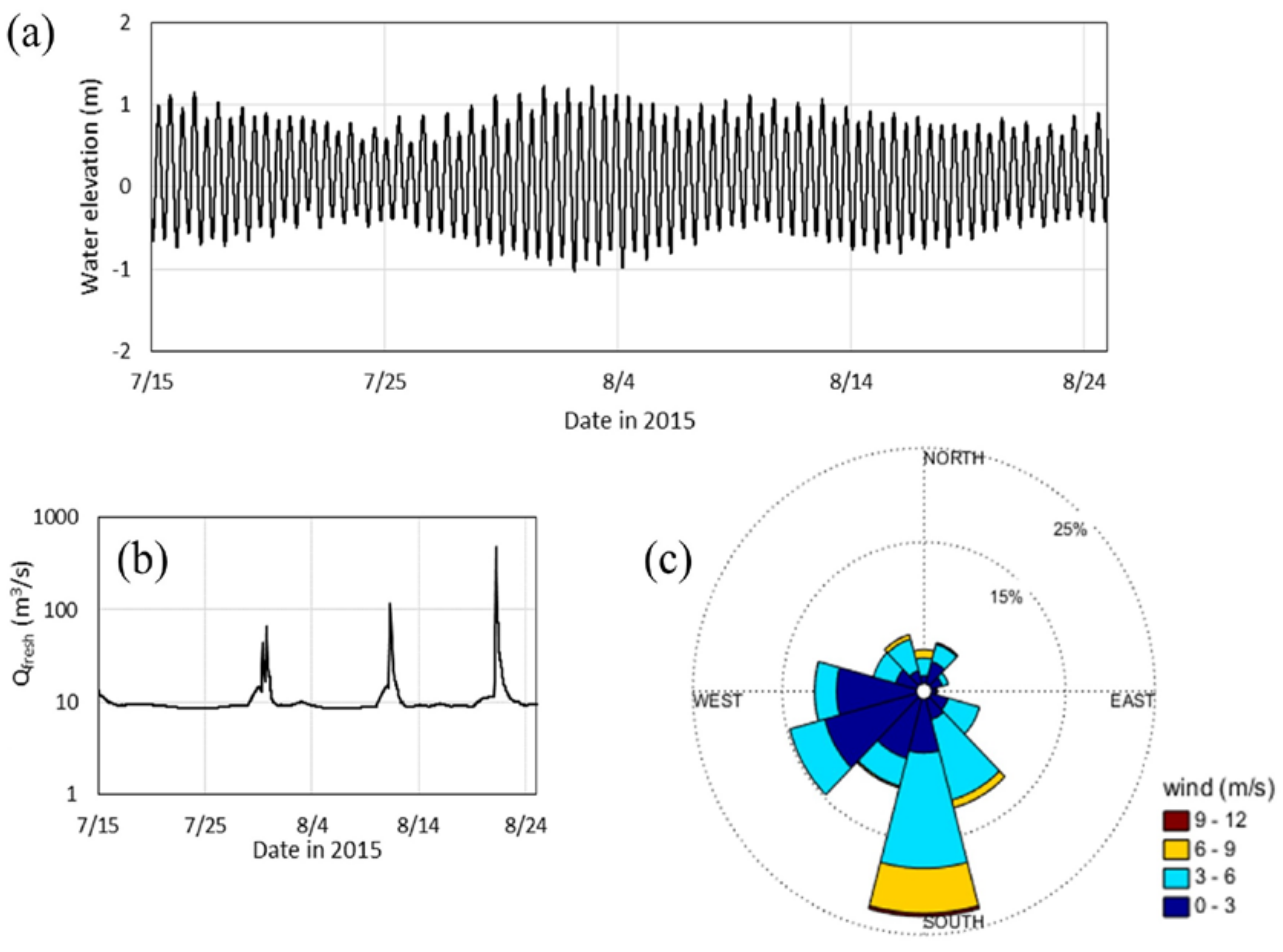
Figure 7.
Vertical profiles of 30-day-averaged velocity at a computational node in (a) North Channel and (b) Beach Channel. The vertical axis represents water depth non-dimensionalized by bathymetry. Streamwise velocity is along the tidal flow’s principle axis. Solid black lines represent results from model ALL (all forcing). Dashed red lines represent results from model NF (no freshwater discharge).
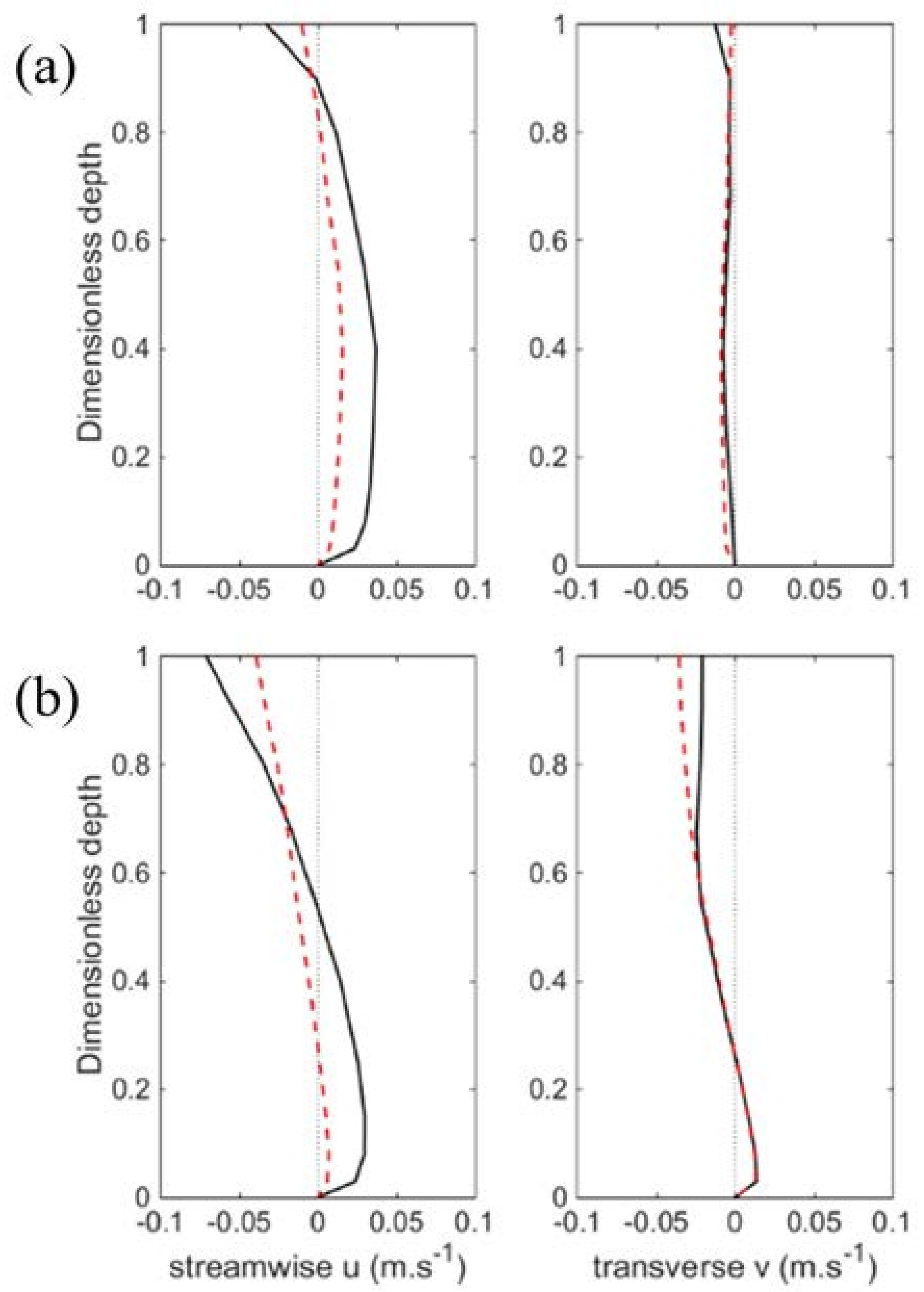
Figure 8.
Snapshots of tracer concentration distribution (tracers were released in Grassy Bay during low tide). The water elevation time series were based on observations at Rockaway Inlet.
Figure 8.
Snapshots of tracer concentration distribution (tracers were released in Grassy Bay during low tide). The water elevation time series were based on observations at Rockaway Inlet.

Figure 9.
Snapshots of tracer concentration distribution (tracers were released in Jamaica Bay during high tide). The water elevation time series were based on observations at Rockaway Inlet.
Figure 9.
Snapshots of tracer concentration distribution (tracers were released in Jamaica Bay during high tide). The water elevation time series were based on observations at Rockaway Inlet.
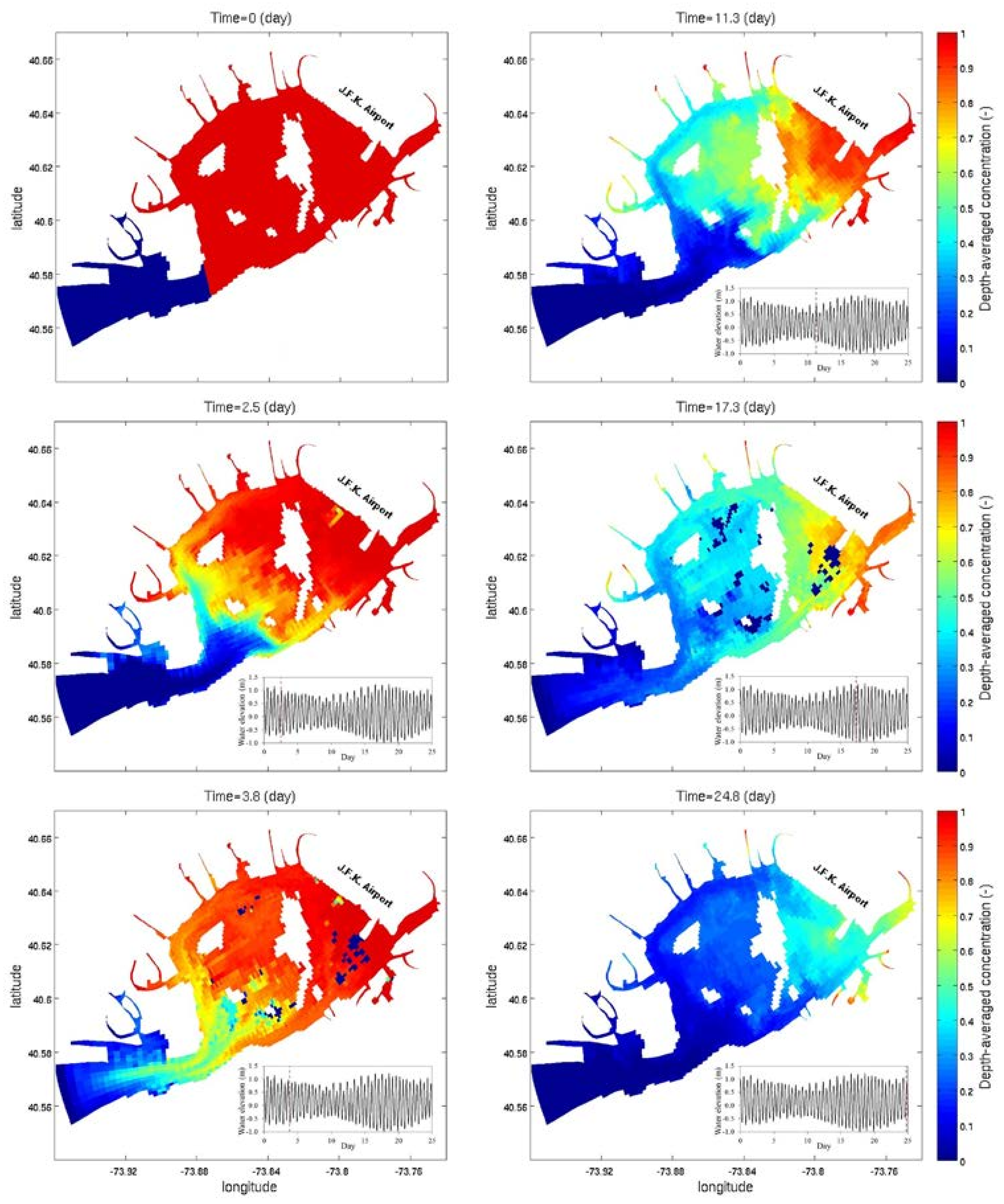
Figure 10.
Time series of the volumetric concentration of tracers in Jamaica Bay (tracers were released during low tide). Concentration was normalized using the initial concentration of tracers. The horizontal dashed lines represent Cv/Cv,0 = 0.37.
Figure 10.
Time series of the volumetric concentration of tracers in Jamaica Bay (tracers were released during low tide). Concentration was normalized using the initial concentration of tracers. The horizontal dashed lines represent Cv/Cv,0 = 0.37.

Table 1.
Statistical assessment of the hydrodynamic model for the 60-day simulation shown in Figure 3, Figure 4 and Figure 5.
| Site | RMSE | Bias | Skill | |
|---|---|---|---|---|
| water elevation (m) | 1 | 0.04 | 0 | 1 |
| water elevation (m) | 3 | 0.04 | 0.03 | 1 |
| usurface (m s−1) | 2 | 0.1 | 0.01 | 0.96 |
| ubottom (m s−1) | 2 | 0.06 | −0.01 | 0.97 |
| vsurface (m s−1) | 2 | 0.09 | −0.01 | 0.93 |
| vbottom (m s−1) | 2 | 0.06 | −0.01 | 0.95 |
| salinity (psu) | 1 | 0.83 | −0.68 | 0.81 |
| temperature (°C) | 1 | 0.94 | −0.29 | 0.83 |
Table 2.
Numerical experiments carried out in the present study to investigate the residence time response to freshwater discharge and wind forcing.
Table 2.
Numerical experiments carried out in the present study to investigate the residence time response to freshwater discharge and wind forcing.
| Model | Forcing | ||
|---|---|---|---|
| Tidal | Wind | Freshwater Discharge | |
| ALL (all forcing) | √ | √ | √ |
| NW (no wind) | √ | × | √ |
| NF (no freshwater) | √ | √ | × |
| NFW (no freshwater/wind) | √ | × | × |
Table 3.
Calculated mean residence times (days), Tr, in Jamaica Bay and Grassy Bay.
| Region | Model | Tracer Release Time | ||
|---|---|---|---|---|
| Low Tide | High Tide | Averaged | ||
| Jamaica Bay | ALL | 20.14 | 15.75 | 17.94 |
| NW | 19.10 | 14.72 | 16.91 | |
| NF | 26.87 | 18.36 | 22.61 | |
| NFW | 25.31 | 17.81 | 21.56 | |
| Grassy Bay | ALL | 11.28 | 10.02 | 10.65 |
| NW | 11.25 | 9.55 | 10.40 | |
| NF | 13.91 | 12.13 | 13.02 | |
| NFW | 15.48 | 13.66 | 14.57 | |
Table 4.
Calculated mean residence times (days) from model ALL and model ALLfts. The percentage difference was calculated as ∆Tr = 100(Tr,ALL,fts − Tr,ALL)/Tr,ALL.
Table 4.
Calculated mean residence times (days) from model ALL and model ALLfts. The percentage difference was calculated as ∆Tr = 100(Tr,ALL,fts − Tr,ALL)/Tr,ALL.
| Region | Tracer Release Time | Model ALL | Model ALLfts | ∆Tr (%) |
|---|---|---|---|---|
| Jamaica Bay | Low tide | 20.14 | 19.08 | −5.3 |
| High tide | 15.75 | 14.70 | −6.7 | |
| Averaged | 17.94 | 16.89 | −5.8 | |
| Grassy Bay | Low Tide | 11.28 | 10.81 | −4.2 |
| High Tide | 10.02 | 9.49 | −5.3 | |
| Averaged | 10.65 | 10.15 | −4.7 |
Table 5.
Tidal prism method’s return flow factor, b, calibrated based on the calculated residence time from sECOM.
Table 5.
Tidal prism method’s return flow factor, b, calibrated based on the calculated residence time from sECOM.
| Region | Model | Low Tide | High Tide | Averaged |
|---|---|---|---|---|
| Jamaica Bay | ALL | 0.93 | 0.91 | 0.92 |
| NW | 0.92 | 0.90 | 0.91 | |
| NF | 0.95 | 0.92 | 0.94 | |
| NFW | 0.94 | 0.92 | 0.93 | |
| Grassy Bay | ALL | 0.84 | 0.82 | 0.83 |
| NW | 0.84 | 0.81 | 0.83 | |
| NF | 0.87 | 0.85 | 0.86 | |
| NFW | 0.88 | 0.87 | 0.88 |
© 2018 by the authors. Licensee MDPI, Basel, Switzerland. This article is an open access article distributed under the terms and conditions of the Creative Commons Attribution (CC BY) license (http://creativecommons.org/licenses/by/4.0/).
Share and Cite
MDPI and ACS Style
Marsooli, R.; Orton, P.M.; Fitzpatrick, J.; Smith, H. Residence Time of a Highly Urbanized Estuary: Jamaica Bay, New York. J. Mar. Sci. Eng. 2018, 6, 44. https://doi.org/10.3390/jmse6020044
AMA Style
Marsooli R, Orton PM, Fitzpatrick J, Smith H. Residence Time of a Highly Urbanized Estuary: Jamaica Bay, New York. Journal of Marine Science and Engineering. 2018; 6(2):44. https://doi.org/10.3390/jmse6020044
Chicago/Turabian StyleMarsooli, Reza, Philip M. Orton, James Fitzpatrick, and Heather Smith. 2018. "Residence Time of a Highly Urbanized Estuary: Jamaica Bay, New York" Journal of Marine Science and Engineering 6, no. 2: 44. https://doi.org/10.3390/jmse6020044
Note that from the first issue of 2016, this journal uses article numbers instead of page numbers. See further details here.