Photogrammetric Surveys and Geometric Processes to Analyse and Monitor Red Coral Colonies

Abstract

This article describes the set of photogrammetric tools developed for the monitoring of Mediterranean red coral Corallium rubrum populations. The description encompasses the full processing chain: from the image acquisition to the information extraction and data interpretation. The methods applied take advantage of existing tools and new, innovative and specific developments in order to acquire data on relevant ecological information concerning the structure and functioning of a red coral population. The tools presented here are based on: (i) automatic orientation using coded quadrats; (ii) use of non-photorealistic rendering (NPR) and 3D skeletonization techniques; (iii) computation of distances between colonies from a same site; and (iv) the use of a plenoptic approach in an underwater environment.

1. Introduction

1.1. Ecological Context and Associated Project

Red coral (Corallium rubrum [1]) is considered an emblematic species for the Mediterranean Sea [2]. Red coral is an invertebrate that grows forming arborescent colonies in rocky habitats from 10 to 800 m in depth (Costantini [3]). With a lifetime of up to 100 years, this species displays a slow growth rate (<1 mm in height per year) with a recorded maximum size up to 50 cm in height [4,5]. Red coral has been fished in the Mediterranean since antiquity for its use in jewelry. As a result of this secular fishing, the current population is characterized by colonies that rarely reach more than 10 cm in height, except in protected areas or in deep water where an unexploited population can still be found.

Moreover, red coral populations are affected by global warming, leading to an increase in its mortality rate. In this context, the red coral is included in the Annex III Protocol Concerning Specially Protected Areas and Biological Diversity in the Mediterranean within the Barcelona convention adopted by the EU through Council Decision 77/585/CEE and classified as an endangered species in the International Union for Conservation of Nature Red List (IUCN 2015).

1.2. Contribution

In this article, we present a set of tools as well as a full methodology dedicated to the application of different technologies for in situ monitoring of Mediterranean red coral Corallium rubrum population. We will describe the pipeline that was set up to characterize the structure and functioning of red coral populations; data collection, either from a multi-view approach implying photogrammetry or from a plenoptic-based method, up to the information processing. In this study, the image acquisition is generally performed by scuba divers. Since diving time is limited and hard to carry out, we chose to use a lightweight setup: a single camera with two strobes for stereoscopic acquisition. We will discuss the different approaches used during in situ surveys that also determine the type of data acquisition. Finally, we will introduce the calibration and orientation methods adopted in each case. These tools provide an estimation of dimensional or geometric characteristics allowing us to explore 3D models of single colonies using sets of photographs (2 to 10) or a plenoptic based acquisition showing the same scene and orthophotographs covering several square meters.

The tools described in this paper are designed to contribute to define efficient management and conservation of red coral populations. Bearing in mind the species’ patchy distribution and depth range as well as the colonies’ complexity and fragility, it is extremely difficult to acquire sound information on key features of the population’s structure and functioning.

To overcome these barriers, we adopted a multidisciplinary approach involving underwater photogrammetry (new study tools and image processing) and biologists (performing in situ acquisitions, statistical and genetic analysis) able to encompass relevant temporal and spatial scales and implementing an innovative analytic tools to obtain quantitative data on the structure and functioning of red coral populations for the very first time.

We contend that this approach will largely benefit the efficiency of management and conservation plans for red coral populations. Particularly in this paper, we will address three main goals:

• Characterization of population structure (scale 1 cm to 50 cm); see Section 3.
• Population dynamics and functioning (scale ${\mathrm{m}}^2$); see Section 4.
• Characterization of colony architecture/complexity (resolution scale 1 mm to 1 cm); see Section 5.

The first goal implies enhanced data acquisition on population size structure. The second goal allows to obtain accurate maps of the surveyed areas (up to $10{\mathrm{m}}^2$) [6]. The third goal addresses a dimensional study, as well as estimating statistical information on common colonies and nowadays rare large-sized colonies. Due to the fragility of corals, all contact should be excluded during the surveys. Thus, the methods developed to tackle this problem should meet several requirements: user-friendly, non-invasive, remote sensing and minimal dive time.

1.3. Short Description of the Surveys Associated with the Presented Tools

In the framework of this study, we have developed a number of tools for monitoring red coral populations and tackling the inherent difficulties through three kinds of surveys that address the previous three goals:

• The first survey aims at performing measurements on randomly chosen populations to characterize the populations. In practice, the underwater site is randomly sampled. Defining an area of interest with a homemade printed quadrat, a plastic frame of size 20 × 20 cm, a scuba diver shoots several photos (distance 20 to 40 cm) with a high overlap ($50\%$ to $70\%$). We opted for a lightweight and practical approach, relying on a single device (a DSLR -Digital Single-Lens Reflex camera- camera) with a housing and two electronic strobes. This multi-view procedure minimizes the diver’s tasks and enables them to easily adapt the measurement procedure to the scene configuration. These photos are oriented in a global frame with an excellent accuracy, thanks to the coded targets drawn on the quadrat [7]. Measurements are directly performed on the photographs using a dedicated graphical interface and the corresponding 3D points are computed. They provide reliable results about the colony size (base diameter, height). Comments on the occurrence of necrosis, for example, can be added.
• The second kind of survey enables the tracking of temporal changes in red coral populations. It gives a fine scale spatial distribution of red coral populations. For these surveys, permanent plots were setup, which allowed for sampling the same areas through time. The plots were marked with PVC (PolyVinyl Chloride) or metal screws embedded in holes of the rocky substratum with epoxy putty. The total covered area varies between 1 and $6{\mathrm{m}}^2$. That area is large enough to monitor hundreds of colonies over time. We used different DSLR cameras embedded in a housing and including two electronic strobes to photograph the transects (from Nikon D70 to D700). We implemented two different sampling methods. The first one consisted of setting a cord attached to the screws to define the plots in each sampling period. Quadrats with coded targets were then positioned above and below the cord as reference. At each position, a few photos were shot and a local coordinate system was defined. The second method consisted of obtaining orthophotos from the permanent plots. Since, in order to build orthophotos, moving a quadrat including coded targets is not possible, we use a global orientation of the scene and for studies at different times, we rely on the whole transect, which always remains fixed, to keep the same coordinate system and compare orthophotos. If biologists really need to sample individual colonies and visualize at the same time the standard of size defined by the quadrat (see Section 3.1), it is still possible to move a virtual 20 × 20 cm quadrat in the scene, using our dedicated application.
• The third type survey implemented was designed for the characterization of emblematic large colonies that have a high natural heritage value (last goal of the paper). The complex shape exhibited by large colonies as well as the entanglement of the branches lead to several problems. Likewise, the proximity of the substrate on which the colony is attached may disturb the analysis. The survey is designed to acquire and build a 3D model first in several ways and then perform automatic measurements on the colonies and determine relevant quantitative morphological information (e.g., like the number of branches). Non-photorealistic rendering based post-processing to smooth the shape, as well as skeletonization methods, were developed.

1.4. Structure of the Document

The paper is structured as follows: first, in Section 2, we will present recent works putting in relation photogrammetry and measurements on living organisms or on the seabed directly. In Section 3, Section 4 and Section 5, each survey will be more precisely described (the photogrammetry approach to measure dimensional data on colonies, the photogrammetric dimensional change monitoring to track the evolution of the populations and finally a study to classify large colonies using plenoptic and photogrammetric approaches). Finally, we will conclude with the contributions brought by the survey methodology developed, based on photogrammetric and plenoptic approaches.

2. Red Coral Surveys

Use of Photogrammetry for Marine Benthic Communities

The surveys applied in this study on red coral are based on standard sampling methods used in marine ecology using quadrats and transects to quantify the abundance and diversity of coral reef communities. Transects are rectangular areas defined by a line deployed over the communities defining the length and quadrats or bars that help to set the width of the transect, the transects can be permanent when marks are setup in the substratum as reference or random if the transects are set in different areas for each sampling. Quadrats are plastic frames allowing for discretization of the observed surface in situ. For instance, Caroline S. Rogers in [8] cites this approach in 1983 and Arthur Lyon Dahl refers to exploited transects since 1917. The use of permanent marks allows observations of change over time. This technique was used for example by Caroline S. Rogers to observe the impact of Hurricane David in 1979 [8].

Indeed, Arthur Lyon Dahl mentioned in [9]: “In 1917, Alfred G Mayor, made a detailed quantitative survey of the fringing reef in Aua in Pago Pago Harbour, American Samoa [10]. Mayor laid a transect across the reef, and counted all the corals and certain other animals within a series of 7.32 m quadrat along the line from the shore to the outer edge of the reef. The transect was repeated using an identical method in 1973 [11] and again in 1980 by the author. Two markers placed on the line in 1973 were still present in 1980, assuring the accurate position of the line”. In this study, we apply the same methods whereas now photogrammetry allows us to be more accurate and exhaustive.

Biologists have integrated photogrammetric computer vision in their fields of research for some years to measure or count underwater living animals or work directly with the seabed. Sanchez et al. [12] used a light photogrammetric approach in shallow water, while Ref. [13] preferred a specifically designed autonomous underwater vehicle (AUV) and Refs. [14,15] relied on specific stereoscopic photography equipment in deep water habitats. Finally, many studies applied photogrammetry to measure benthic communities [16,17,18,19] and also [20]. Shortis [21] provided a clear and synthetic overview.

Underwater photogrammetry has a drawback since geolocation can be difficult. However, the need to use a geographic information system (GIS) is still a reality. Actually, a local coordinate system can be defined [22,23]. Photogrammetry and GIS approaches can be used to characterize reproductive units within red coral populations by studying family relationships by combining spatially explicit positions with genetic analysis [24]. Contrary to traditional methods used in marine biology, which can be destructive and difficult to be implemented, photogrammetry is non-invasive and can be performed in situ [25]. Moreover, the emergence of powerful photogrammetry processing software, like PhotoScan [26], has changed the way to handle these studies. This approach is now more user-friendly for non-specialist researchers [19]. Finally, photogrammetry is being perceived as a useful and affordable approach for an increasing number of research teams. See, for example, Refs. [27,28,29] or the study of structural complexity of underwater seafloor [30,31,32]. GIS software is also coupled with photogrammetry in [33] for a deep coral survey.

Some stereo tools, diver-operated or embedded in an AUV, have been developed since some years ago, in the field of underwater robotics in order to easily survey a site using photogrammetry with specific methods to manage the stereo systems and local bundle adjustment. These developments were intended to support inclusion of bathymetry in an underwater archeology context as well as in marine biology (see [32,34,35,36]). Similarly, we have also developed our own low-cost system, which is easier to use in complex environments [37]. The system is based on embedded and distributed low-power mini computers (Raspberry Pi). A set of software programs developed by our team ensures a general good precision with local bundle adjustment and real-time odometry. Moreover, a bridge was done with the commercial application Photoscan developed by Agisoft (Saint-Petersbourg, Russia) [26].

Today, many new and complex applications merge several media, lidar and photogrammetry as well as using mobile systems such as aerial drones, remotely operated underwater vehicles, etc. [38]. However, what we can see in this brief overview of methods used to make an underwater survey of coral reef colonies is that, even if the use of photogrammetry has dramatically increased over the last five years, the main goal of these surveys can be achieved only by human observations.

Indeed, the knowledge required to interpret the information is the key point of the survey. We will focus in this paper on several methods and techniques to automate partially the 3D acquisition and the morphological information acquisition. Compared to the previous works quoted in this section, we offer here different dedicated interfaces (e.g., user-friendly graphical user interface, implementation of photogrammetry algorithms, development of our own bundle adjustment, including specific constraints on distances on the quadrat to benefit from an optimal orientation quality...). The final survey should be done by the biologists and the main contribution of the approach described in this paper is to be able to minimize the time spent underwater (data acquisition) and to be able to optimize the analysis of the accurate and quite exhaustive 3D data (in several formats: 3D models, point clouds, color map) in the laboratory.

3. Semi-Automatic Coral Measurements and Quadrat Sampling

In order to characterize population size structures, we developed a semi-automatic processing chain based on photogrammetry. First, colonies are randomly sampled using a 20 × 20 cm plastic quadrat. This quadrat will be used both to scale the future model and set up a coordinate system. The whole process can be divided into five steps.

3.1. Setting Up the Quadrat

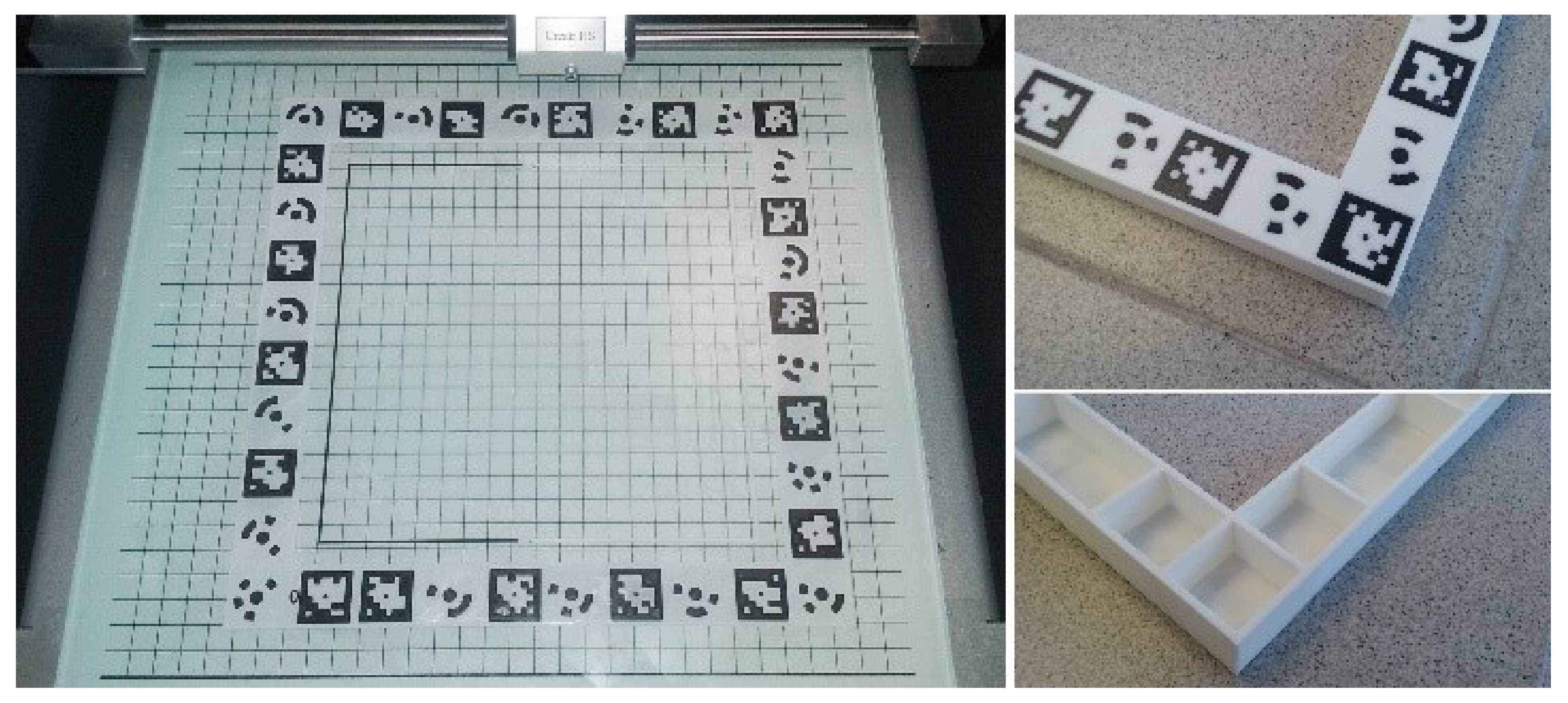
The quadrat is a homemade 3D printed plastic frame that can be easily made by anyone that has the 3D mesh file. This mesh file is designed to comply with the standard used by biologists. The frame’s internal dimensions were fixed to 200 × 200 mm. The external dimensions were chosen to ensure a good visibility of the targets: 230 × 270 × 15 mm. It incorporates two kinds of coded targets. First, 18 classical circular targets used by Photoscan and Photomodeler software—second, 18 square targets from the TagRuler system, which we have developed for our own photogrammetric platform ARPENTEUR [7]. The presence of these two kinds of targets enables processing the photos both in the commercial software and in our own photogrammetry modules. The 18 targets of each type are evenly distributed on the frame. Their location is precisely known and they can be used as control points. The shape of the quadrat itself, designed with CAD (Computer-Aided Design) techniques, takes into consideration underwater constraints; no air pockets, thickness of 2 mm and cellular framework to balance stiffness, weight and handling (see Figure 1).

3.2. Shooting Methodology

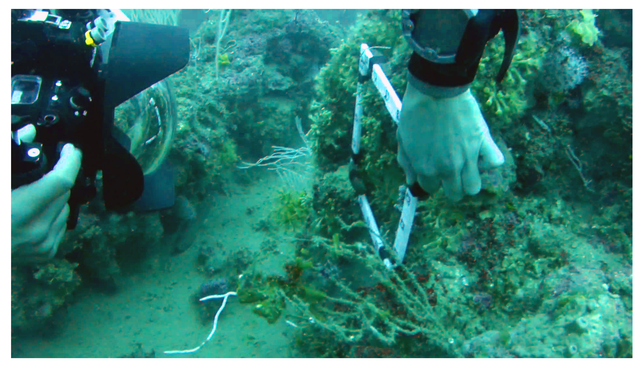
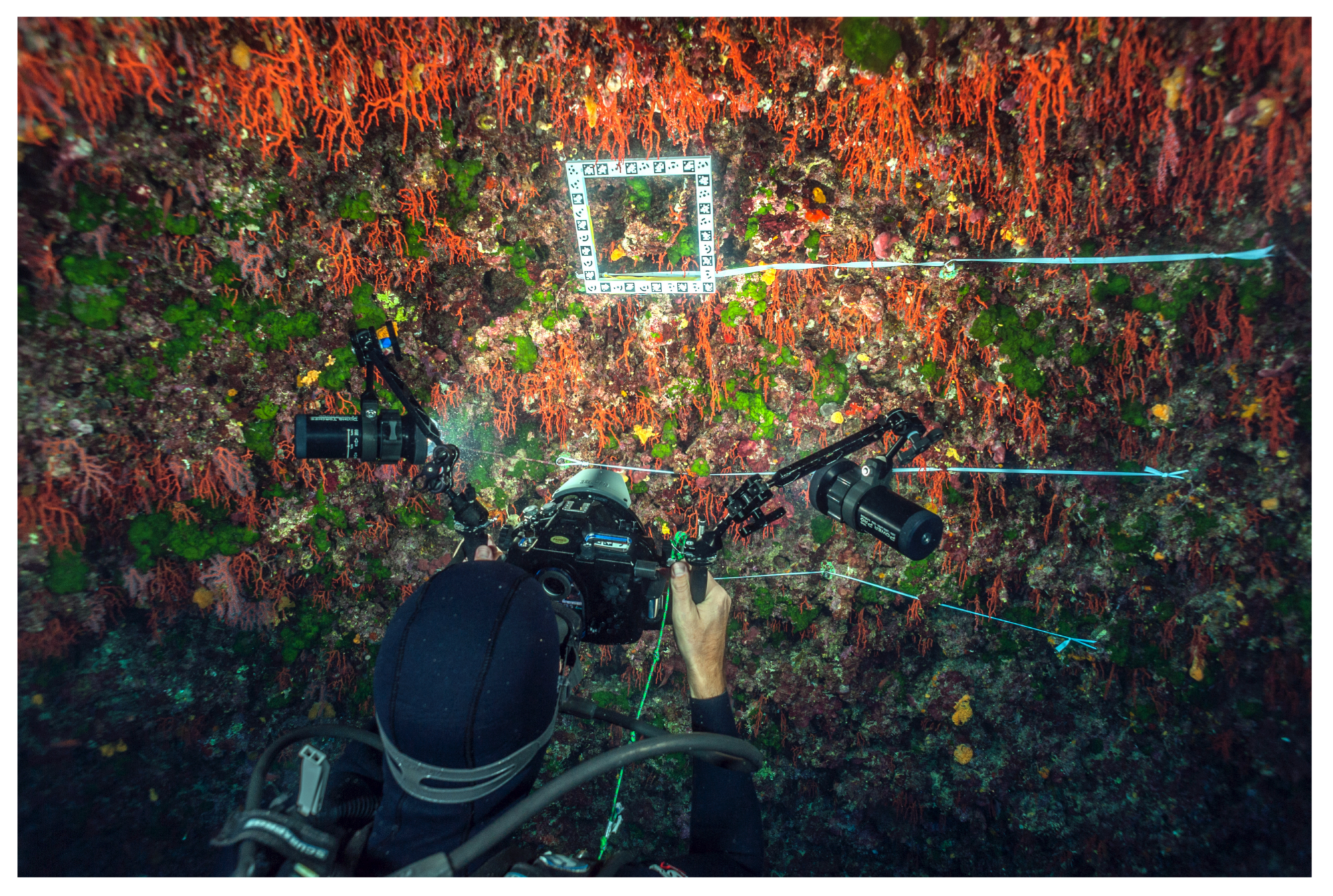
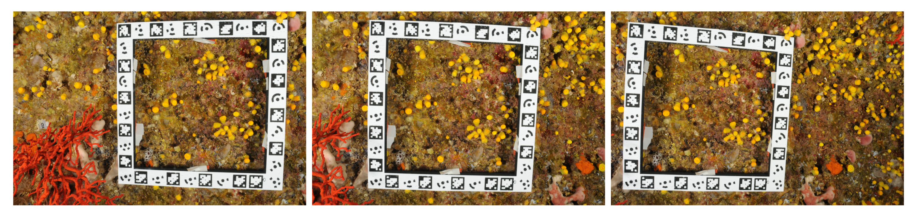
In practice, the printed quadrat is placed on the seabed (see Figure 2), or attached to buoys (embedded in the quadrat) on a cave ceiling or sometimes held in place by another diver (see Figure 3) who keeps it stationary with respect to the seabed. Then, between two and ten photographs are shot (but more generally, three are enough), so that the common covered area and the base are maximized (see Figure 4). Due to the difficult constraints of manned underwater acquisition (limited time, limited visibility, instability, etc.), this approach is easy to carry out and minimizes the number of photos and the processing time (see the next subsection).

3.3. Automatic Orientation

The photo orientation procedure is used to determine the pose (position and orientation) of the camera used for each capture (called external or exterior orientation). This is essential to be able to estimate and measure the 3D structure. In contrast to structure-from-motion (SfM) scenarios, no camera calibration is required in advance. However, we mention that using calibration parameters avoids introducing more degrees of freedom in the optimization phase and leads to more robustness in our case. The camera parameters (referred to as interior or internal orientation) are estimated jointly with the exterior orientation in a closed-form manner, more accurately than self-calibration approaches.

Each single camera shot is enough to recover the interior and exterior orientation, and also the distortion coefficients, both radial and tangential. This is done based on Tsai’s camera calibration scheme [39] adapted to planar targets as summarized below.

The photo orientation procedure is applied to each captured image separately at first, and then the recovered parameters are used as initial values in a further optimization phase. We consider that each photo contains the image of the quadrat with TagRuler or circular markers (with the region of focus at the center); here, five points are enough to recover all the parameters, but more points provide better accuracy. A robust TagRuler and circular marker detection are developed based on the AprilTags open-source project. The detected points together with their known relative position serve as input to the recovery procedure. Formally, using a pin-hole camera model, a 3D point ${\mathbf{P}}_{\mathbf{c}}={\left[X_C{Y}_C{Z}_C\right]}^{\top }$ in a camera coordinate system is projected to a 2D point ${\mathbf{p}}_{\mathbf{I}}={\left[x_I{y}_I\right]}^{\top }$ in image coordinates as

$$x_I=f\frac{X_C}{Z_C}\mathrm{and}{y}_I=f\frac{Y_C}{Z_C},$$

(1)

where f is the focus distance (in general, the ratio of the pixel dimensions parameter must be considered. It is not taken into account here as most modern cameras have square pixels). Using the ratio of both equations yields a result that is independent of the focus distance and distortion

$$\frac{x_I}{y_I}=\frac{X_C}{Y_C}.$$

(2)

Transforming ${\mathbf{P}}_C$ from world coordinates is achieved with the mean of a rotation matrix $\mathbf{R}$ and translation vector $\mathbf{t}={\left[t_x{t}_y{t}_z\right]}^{\top }$ (external parameters)

$${\mathbf{P}}_C=\mathbf{R}{\mathbf{P}}_W+\mathbf{t}.$$

(3)

By considering the origin of world coordinates at one corner of the quadrat, we can consider $Z_W=0$ for all control points. After the expansion of the last equation and the substitution in Equation (2), we obtain:

$$\frac{x_I}{y_I}=\frac{r_{11}{X}_W+r_{21}{Y}_W+t_x}{r_{21}{X}_W+r_{22}{Y}_W+t_y},$$

(4)

where $r_{ij}$ is the element at row i and column j of $\mathbf{R}$. This yields after simplification to a linear equation with six unknowns; $r_{11},r_{12},r_{21},r_{22},t_x,t_y$. For each 2D–3D correspondence point, we obtain one such equation. Using a least-squares approach to solve this equation, the obtained solution is up to scale. By applying the orthogonality constraint of a rotation matrix, we could simultaneously recover the five remaining elements using orthonormal equations. Hence, the focal distance and $t_z$ can be recovered using Equations (1) and (3).

The next step is to use the computed parameters as initial values in a nonlinear optimization phase. Since the origin of the coordinates is considered to be the same for all photos, the recovered external orientations are passed to the optimization step untouched. The focal distance, which is the only recovered internal parameter, is averaged for all photos. The principle point is initialized at the center of the image. Finally, we optimize the values for all external, internal, and distortion parameters using the Levenberg–Marquardt method and the reprojection error:

$$\sum _N^{i=1}{(x_{Ii}-x_{Pi})}^2+\sum _N^{i=1}{(y_{Ii}-y_{Pi})}^2,$$

(5)

where $(x_P,y_P)$ are the coordinates of the re-projected point using estimated parameters. Considering that the working distance is approximately 200 mm, the residuals obtained on the control points are generally less than 1 mm.

3.4. Red Coral Colonies’ Measurements

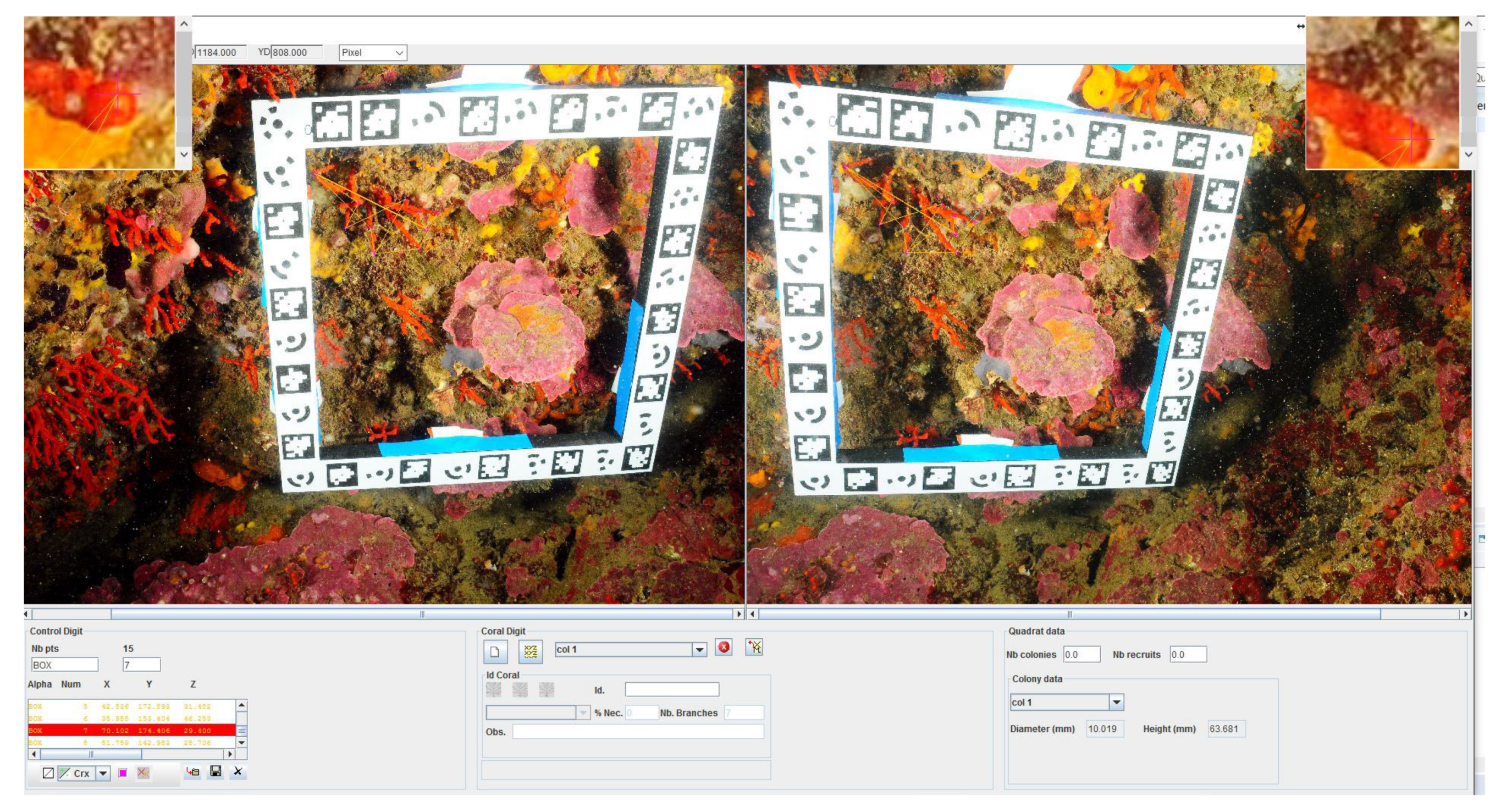
We developed a fully functional graphical user interface (see Figure 5) that enables us to perform measurements on the colonies inside the quadrat. The interface allows the presentation of two photos side by side (chosen by the operator from the set of photographs taken on-site and regarding these colonies). The user selects homologous points on the photos, so that the resulting 3D point is computed by triangulation. The interface performs real-time controls to ensure the integrity of the data, for example, correlation to ensure the quality of the chosen pair of points. Finally, the user has the possibility to determine various information including the diameter of the base, maximum height and approximate volume as well as visual observations, such as the percentage of necrosis for each colony and the density of colonies and recruits.

A set of tools is available within this software and allows for constraining the homologous points determination, displaying the epipolar line, performing automatic cross correlation, and contrasting evaluation, local zoom, dynamic residual visualization, etc.

3.5. Computation and Results

The results are calculated in a matter of a few seconds. The results are exported into standard widely used file formats (XML, Excel, PLY and VRML to visualize the point cloud resulting from the measurements) to fit the tools already used by biologists for their analysis.

Very recently, photogrammetric results and coral measurements have also been exported according to an ontology developed in the LIS laboratory in the framework of the ARPENTEUR project [40].

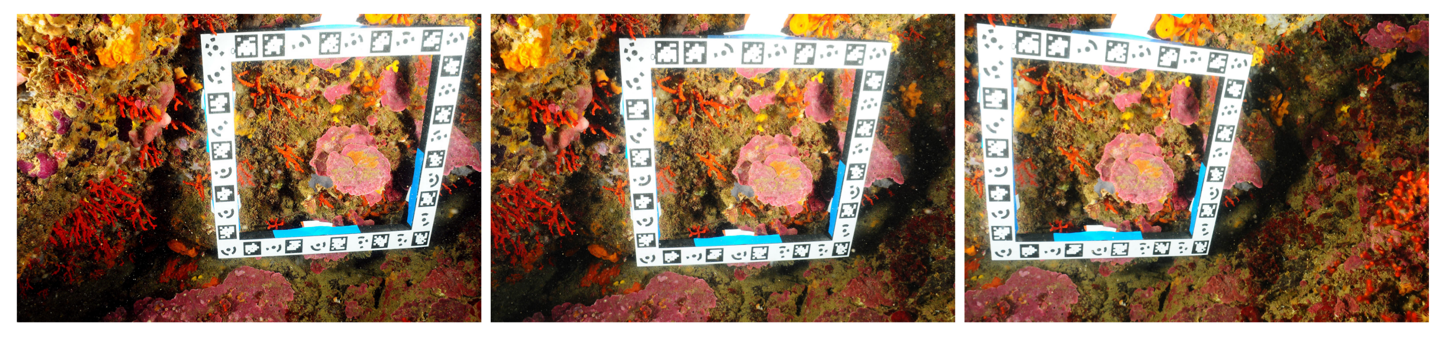
Below, we provide numerical results on an in situ study case to assess the quality of the measurements performed. We shot three photographs with a Nikon D300 (focal 20 mm, resolution: 4288 × 2848). The pictures are shown in Figure 6.

Two kinds of analysis are carried out: first, the reprojection residual (pixel unit) on the 36 coded targets present on the quadrat; next, the difference between the computed distances in mm between all the targets and the theoretical ones given by the coordinates of the control points (called an accuracy). For each case, the different error indicators computed are the average, the root mean square error (RMSE) and the median error. The results are shown in

Table 1. Residual analysis.

	Reprojection Residual (Pixels) for 36 Ground Points	Residual on Distances (mm) or 544 Computed Distances
Average	1.10	0.34
Median	1.07	0.41
RMSE	1.21	1.64

.

The reprojection residual, which we call a precision, are in the range of one pixel, which is a fairly good result, considering the additional constraints added underwater (mainly, distortion correction).

Concerning the distances, considering that the interior of the quadrat is a 20 cm square, the average distance error computed is less than 0.5 mm.

4. Estimation of the Temporal Changes and the Colony Spatial Distribution

The goal of this study is to determine the changes over time in the red coral populations. This implies both studying colony changes over time and also correlating genetic studies with the spatial position of colonies to better understand the mechanisms involved in the populations functioning (reproduction and recruitment).

Initially, we used a different process that relied on surveys of permanent plots, set up using PVC screws fastened to holes in the (rocky) substratum with epoxy putty. The pattern of this grid (number of transects and distances between the screws) varied, depending on the kind of substratum and microtopography. Then, areas were squared off using elastic cords to define normalized sampling areas. Then, transects were photographed, using different cameras (Nikon D70, Nikon D300) within housing and two electronic strobes. On each sampling area, the 200 × 200 mm quadrat was positioned (above and below the cord length) and two or three photos were shot using slightly different angles (about ${30}^{°}$). Notice that the covered area generally did not exceed 2 to $6{\mathrm{m}}^2$. Nevertheless, it enabled us to monitor hundreds of colonies.

This acquisition process was heavy to carry, slow and limited, considering that it did not enable us to efficiently monitor spatial changes on the colonies.

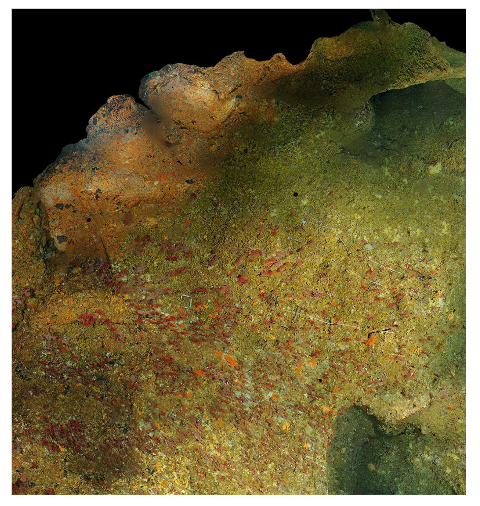
Thus, we decided to use a different acquisition method that consists of positioning the quadrat at a given place. The first step is to shoot a large collection of photos of the area (generally, hundreds to thousands). These photos are taken by advanced divers, who efficiently cover the area and keep the same distance between them and the colonies, so that the light variations are minimized. Next, the set of photos can be oriented in a global system of coordinates given by the quadrat (here, global does not refer to a world geographic reference system, but rather means that we have a unique coordinate system for all the covered area, scaled thanks to the quadrat), which leads to a sparse point cloud. At the same time, the scale is also applied. The next step computes the dense cloud. Alternatively, this dense cloud can be meshed, to produce a high-resolution 3D model. Finally, the most important step is building the orthophoto for each sampled area. From a suitable plane of projection, the previous 3D model is projected using an orthographic projection. This projection conserves distances, so the resulting orthophoto has the same scaled coordinate system attached as the one used by the mesh and the point cloud. During the monitoring process, biologists require estimating distances between colonies and quantifying temporal changes. Considering the goal of this study, orthophotos perfectly fit their needs. They offer a global view of the area (see Figure 7 for an example), with a very high resolution, while pixels are related to the true coordinates. Moreover, it is easier to work with orthophotos than with 3D models, which are not as handy to use.

4.1. Orthophoto Measurements

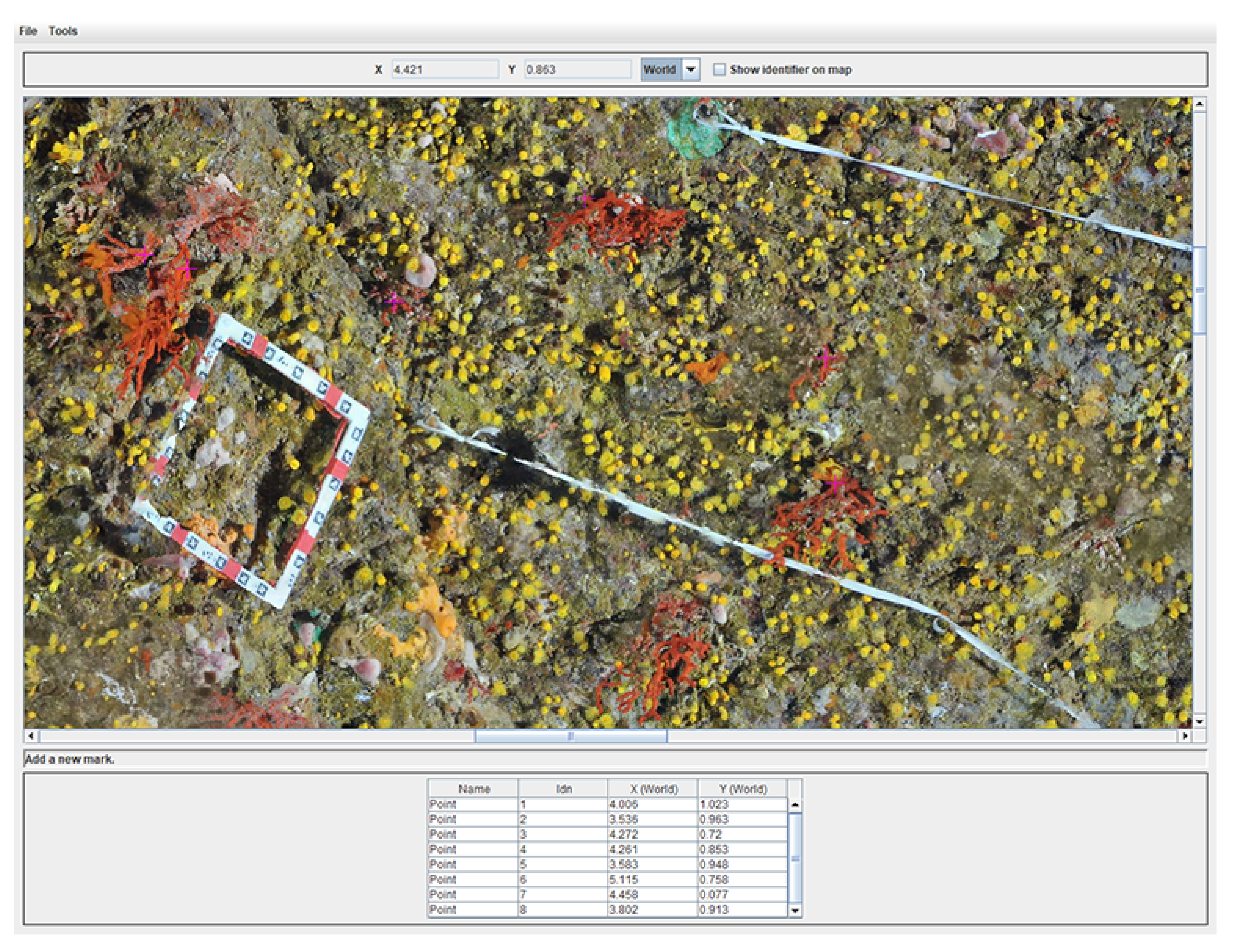
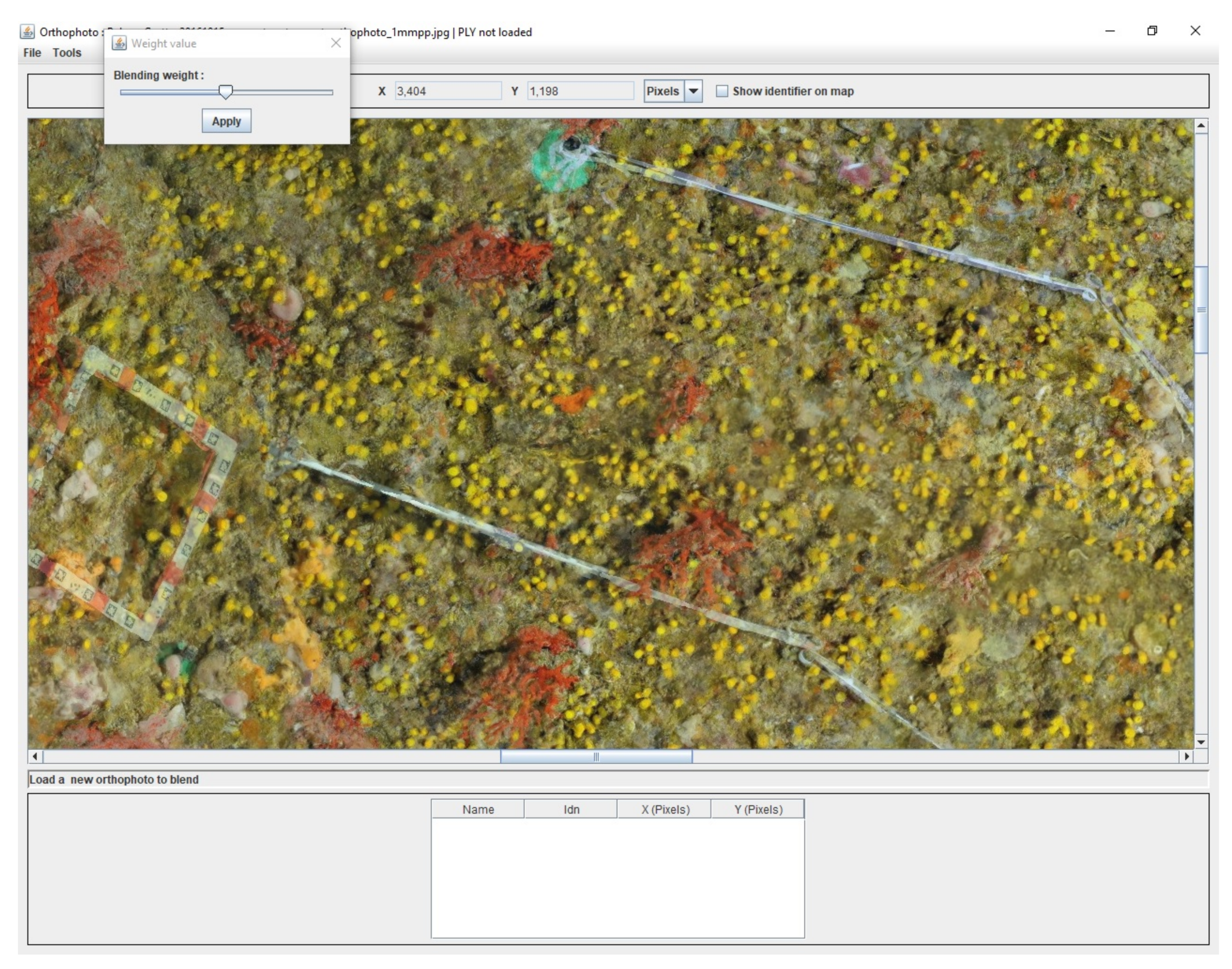
As a consequence, we developed an efficient dedicated software enabling us to load an orthophoto and pick points on it. It offers the possibility to perform measurements on selected points. The user can directly select interesting points on the orthophoto. The upper part of the application shows mouse coordinates in world units, while the bottom part summarizes the set of measurements already done. This point list can be managed (add, remove, edit, etc.). Moreover, in order to handle large-dimension orthophotos, they are divided into small blocks, which are merged in a transparent way for the final user. Finally, the distance map between all points can be computed. We provide an example of the user application in Figure 8.

We tried different methods to provide distance estimations. Due to the ruggedness of the seabed, Euclidean distances led to poor results, as they did not take into consideration the sea floor’s topography.

Several methods have been developed to compute exact or approximations of the shortest path on graphs. Dijkstra developed a well-known algorithm to solve this problem in [41]. On a triangular mesh, this algorithm computes the optimal path that follows the ridges of the triangles, but it is slow on large meshes, as it needs to test every vertex present.

Dijkstra’s algorithm enables a good approximation of a distance along the curve of the ground, provided the mesh is dense enough. However, there are two main problems. First, the computation time depends on the size of the mesh. Some improvements can be found in the literature to speed up the computation, like the A* algorithm [42]. The counterpart is that the resulting path may not be the optimal one. In our case, we use a slight improvement of Dijkstra’s algorithm: the list S is filled at runtime with the vertices discovered and not studied yet, instead of being totally filled at the beginning. The second problem concerns the computed distance, which can be over-estimated in some cases. As the path follows the edges of the triangles, the meshing pattern can have a noticeable influence on the result. To provide the best fit of the desired distance, we decided to move to a geodesic-based algorithm (Algorithm 1). In this case, the estimated curve goes through the faces of the triangles, so that the meshing pattern and even the mesh density have a lower influence on the accuracy of the result. Several methods approximating the geodesic curve exist in the literature [43,44,45]. The one we have developed is based on the Darboux frame [46]. The method is initialized with the path estimated by the Dijkstra’s algorithm. Then, the vertex positions are slightly moved to fit the geodesic curve. This is a good choice, as the path returned by Dijkstra is close to the geodesic one.

Algorithm 1: Geodesic algorithm

Data: Input data are the point list given by the computation of the Dijkstra path L, composed of a set of N points coinciding vertices ${\mathbf{m}}^{\left(i\right)}$ from the mesh, such as: $L:\{{\mathbf{m}}^{\left(i\right)},0\le i\le N\}$.   Result: A list containing the geodesic path sampled.   while current iteration ≤ max iteration do      end

To determine the 3D coordinates of the starting and ending points selected from the orthophoto, we have to do a few calculations. Knowing the plane of projection used to project the 3D model (generally the $XY$ plane to simplify), we trace a ray from the $(x,y)$ chosen point, with a direction equivalent to the normal of the plane (Z-axis if the plane is $XY$). The intersection between the ray and the triangles of the mesh corresponds to the requested 3D point. This search can be time-consuming, as it depends on the mesh size, so we decided to accelerate ray-triangles intersections using a primitive-based partitioning algorithm. While different methods exist in the literature, they are mainly divided into two categories: space partitioning algorithms, including octrees, kd-trees,... (see for example [48,49]) and primitive-based partitioning algorithms ([50,51]). This second category especially includes BVH (Bounding Volume Hierarchy). Recently, this approach has become increasingly popular in the ray-tracing community. It is, for example, used in the highly optimized library Embree, developed by Intel (Santa Clara, CA, USA) [52,53]. This is also the choice we made, as it is not really difficult to implement.

Finally, the key advantage of the presented tool is that it offers a handy graphical interface, enabling tracking of coral colonies and performing accurate 3D distance computations, while hiding the complex part of this computation step from the end user.

4.2. Visual Temporal Changes

Another useful tool was developed to visualize the evolution of the populations over time. It takes advantage of the fact that transects remain in place for the photogrammetric studies at different times. Thus, the orthophotos can be oriented in the same coordinate system. An example is provided in Figure 9. Moreover, the weighting value to blend the two images can be changed on the fly.

5. Inventory of Red Coral Colonies

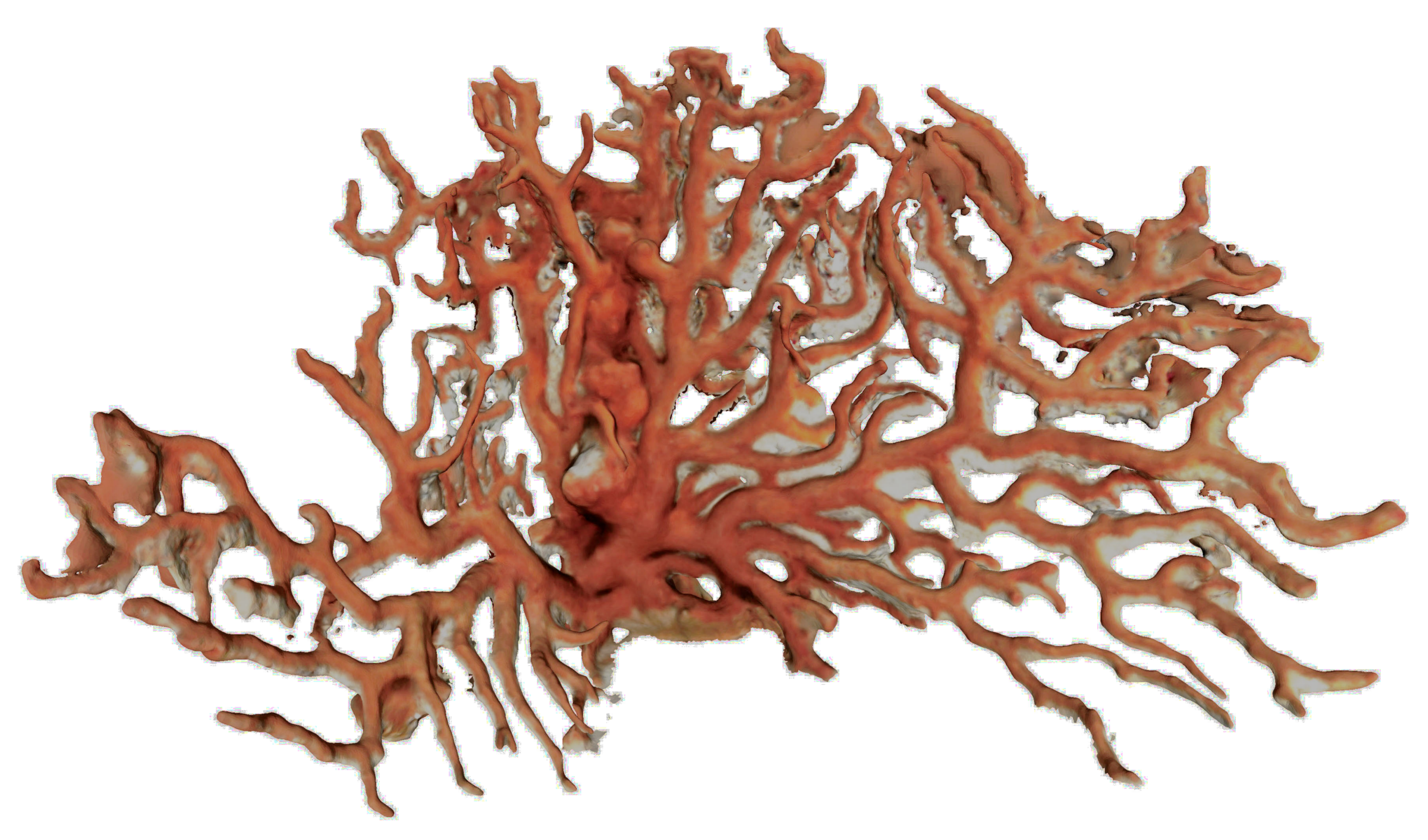
The third goal of the paper is to develop tools to characterize structurally complex red coral colonies in view to build a library of emblematic colonies. The tools developed modeling the colony and extracting from it relevant information, like morphological ones. Large colonies are particularly noticeable, as they exhibit complex shapes with multiple branches. Their structure and the acquisition context make this problem very challenging both for a human or an automatic-based analysis. We will show in this section the adopted methodology and solutions leading to appropriate and workable results. We rely on different kinds of tools to provide data from different sources. The global process can be divided into two steps: data acquisition and extraction of relevant information. The acquisition was carried out in situ, for the majority, but also in the lab on dead coral colonies that are held in public or private collections.

5.1. Photogrammetric Acquisition

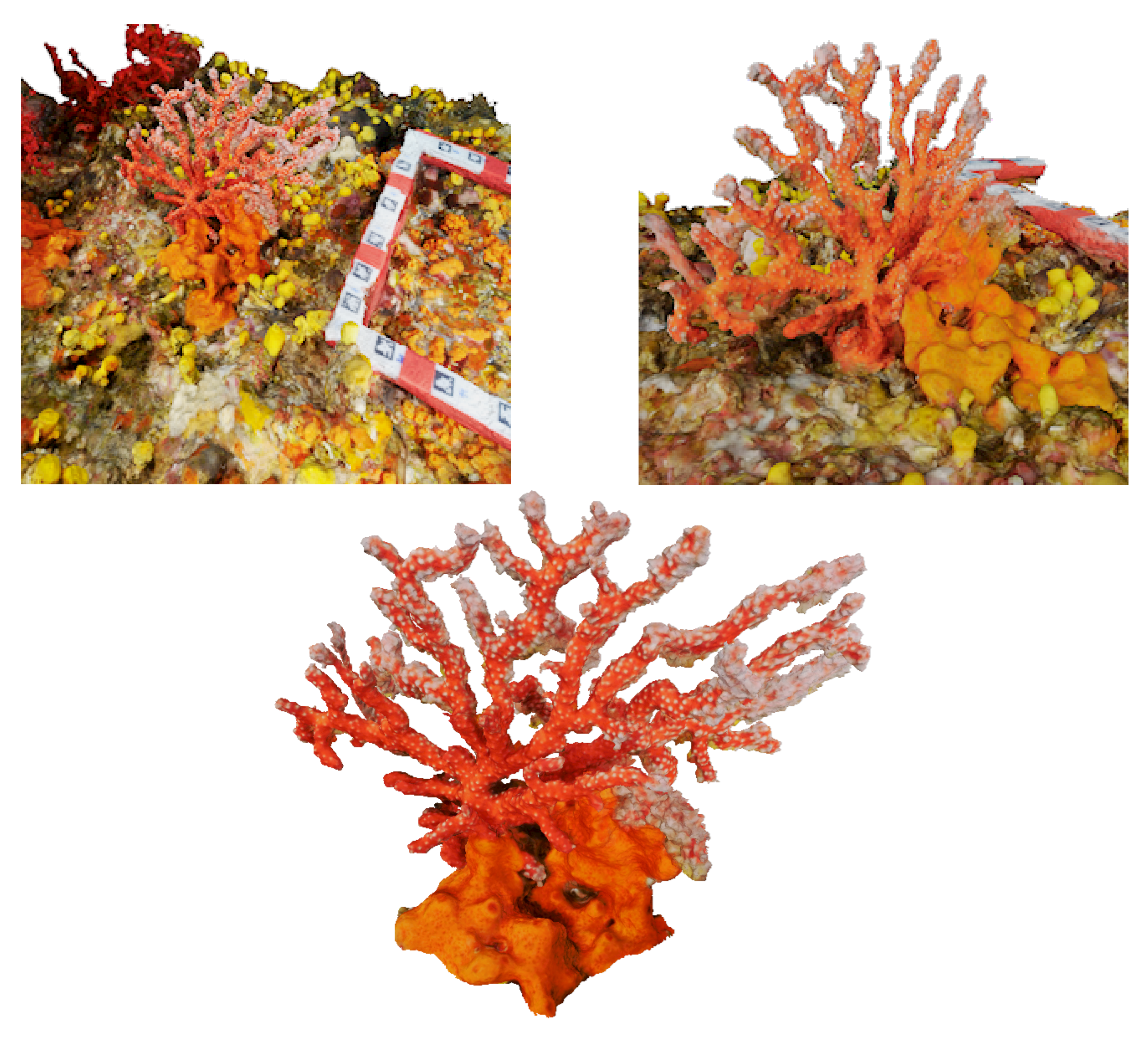
The classical photogrammetric approach is achieved by shooting hundreds of photos, with a high overlap. As said previously, the density of large colonies multiplies hidden areas. A photogrammetric acquisition relies on the redundancy of data, ensured by the redundancy of the areas’ shots. The more complex the colony, the more photos we should take and the less missing data we get in the reconstruction process. Moreover, red coral colonies grow in dark and narrow areas, like cave ceilings, which present a complex topography. This makes the photogrammetric acquisition process challenging and time-consuming. In a practical way, it is generally performed by a scuba diver. We tested both HD (Olympus TG2 and Canon G1) and reflex cameras (Nikon D700 and Nikon D300). The whole process enables computation of the 3D point cloud, and, next, the mesh based on the dense cloud. See examples of acquired large colonies in Figure 10 and Figure 11.

5.2. Non-Photorealistic Rendering (NPR)

The next step consists of extracting relevant data from the mesh modeling the colonies. We first developed an automatic tool based on NPR (non-photorealistic rendering) [54]. NPR is a method that highlights contours, ridges or valleys and enables detection of noticeable points. The main advantage is that it uses information that is not available on images: the surface normals. Basically, the principle reads as following: consider a 3D model observed from a given point of view. For each vertex, we define the normalized vector $\mathbf{v}$ to be the vector from $\mathbf{t}$ to the viewpoint. We call $\mathbf{n}$ the normalized normal at vertex $\mathbf{t}$. Then, we can compute the following scalar quantity resulting from the dot product:

$$\begin{array}{c}\hfill I\left(\mathbf{t}\right)=\mathbf{v}\left(\mathbf{t}\right)·\mathbf{n}\left(\mathbf{t}\right).\end{array}$$

(10)

Ideally, the set of vertices such as $I\left(\mathbf{t}\right)=0$ represents the contour. To be less restrictive due to the acquisition noise and to extract more parts of the relief, it is a good idea to add a threshold, say $th$, so that we can keep suggestive contours. These suggestive contours are then defined by:

$$\begin{array}{c}\hfill I\left(\mathbf{t}\right)<th.\end{array}$$

(11)

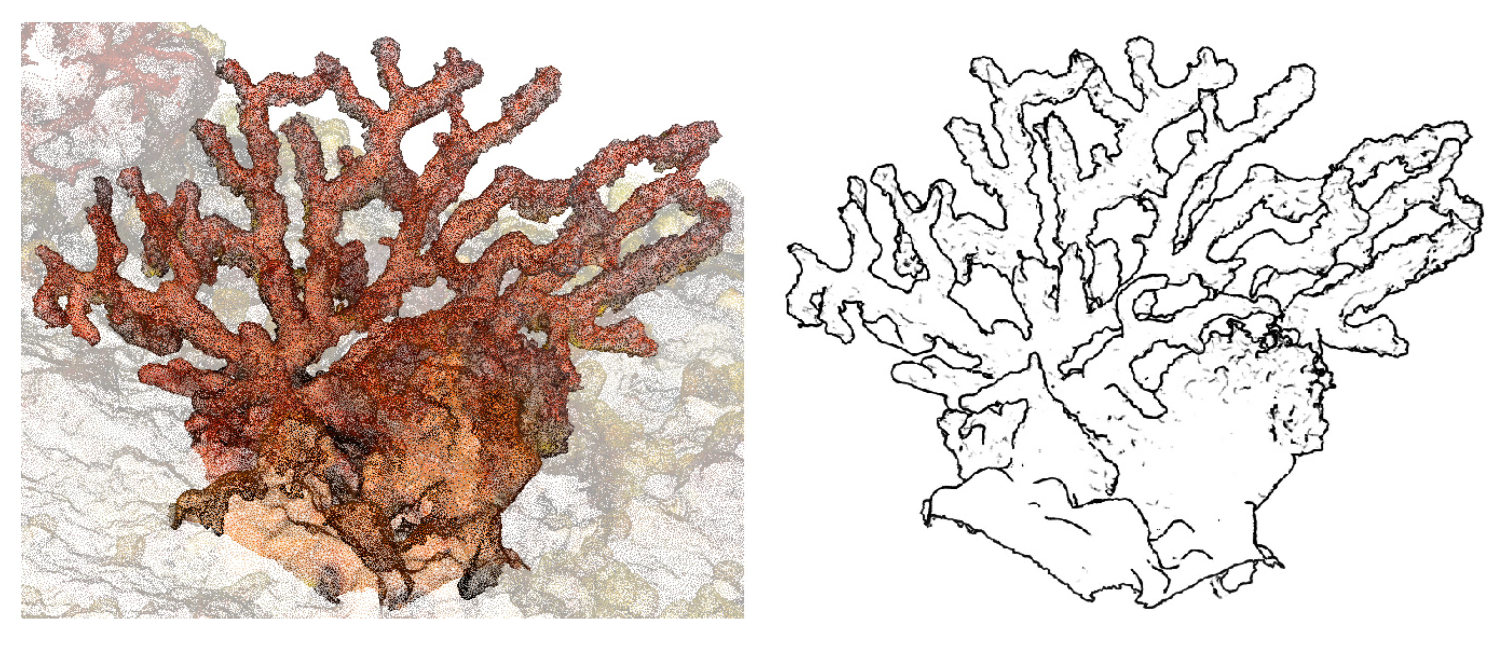
More formally, the suggestive contours are defined as the set of minima of $\mathbf{v}·\mathbf{n}$ in the direction of $\mathbf{w}$, where $\mathbf{w}$ is the projection of the view vector onto the tangent plane. An NPR representation of a colony is given in Figure 12.

Hence, the NPR processing we use corresponds to the 3D contours from a given point of view. One way to obtain an accurate representation of these contours consists of oversampling the resulting image of contours, with a ray-tracing based method. For each contour pixel, a ray that passes through the pixel is cast from the camera. The intersection with the 3D mesh is tracked. By subdividing the pixels, an oversampled representation of the contours of the 3D model is obtained.

From four different viewpoints, the global shape of the model is extracted. This shape can be meshed again, so that we obtain a simplified representation of the colony, where the noise resulting from the acquisition has been smoothed. This process is important for the next step.

5.3. Skeletonization

5.3.1. Getting the Skeleton

Manual extraction of morphological information on large colonies, such as the number of branches or diameter of each node, is a difficult task, even if it is not directly carried out in situ, as the populations show a really complex shape. Furthermore, working on the photos resulting from the acquisition process would not lead to good results, even in the case of an automatic process, because of the occultations. This also motivated our choice to use an NPR-based approach, as it is the best way to determine the true contours, taking into account that some branches hide the rest of the geometry.

We propose in this section an automatic process for the extraction of morphological data. Now that we have an accurate and well-defined model of the coral colony, the idea is to apply skeletonization algorithms to extract the shape and obtain an analytic representation. With the skeleton, we will be able to localize the different parts of the colony and automatically count the number of branches or other associated dimensional data. Many methods for skeletonizing shapes exist in the literature. Few methods lead to a 3D skeleton, as the majority of the works are based on images [55,56,57,58]. Historically, the concept of medial skeletons was introduced for 2D shapes. It was primarily a way to reduce the amount of data necessary to describe the topology or symmetry of the shape. The concept was later extended to 3D shapes [59]. This yields new difficulties, as the desired skeletons are more rich and the shapes more complex, making this problem challenging.

In a general way, a medial skeleton meets several definitions. For a non-exhaustive list, we can write:

• The medial skeleton is the set of ball centers with the maximum radius inscribed in the shape.
• Setting a fire that propagates from the boundary to the center of a mesh, the medial skeleton is the set of points where the fire fronts meet.
• Reformulating the last definition in terms of distances, the medial skeleton is the set of locations with more than one closest point on the boundary of the shape.

For 3D shapes, the best families of skeletons that both extend the concept of wireframe of an image for volume and could be directly used on corals are the curve-based skeletons.

We decided to implement the method described in [60]. Liu et al. developed a robust algorithm to skeletonize noisy mesh that preserves connectivity. Their work is based on iteratively thinning on cell complexes. A cell complex is a closed set of k-cells. For example, a cube is a 3-cell, a rectangle is a 2-cell, its edges are 1-cell, and its vertices are 0-cell. An easy way to build the cell complex from a triangular mesh is to use classical methods to first turn it into a voxel representation. Then, 0-cells are all the vertices, 1-cells are the all the edges and so on. Each kind of cell enables characterizing a particular shape. 1-cells are useful at describing tubular shapes, which perfectly fits our needs. Regarding the definition of a medial skeleton in a thinning-based algorithm, it corresponds to the simulation of the way a fire propagates. The key in their method is to compute a global indicative value, the medial persistence, which characterizes how long a discrete cell persists in an isolated form. We briefly describe how the skeleton is created below:

The algorithm takes place in two steps. First, an iterative thinning process is performed and the medial persistence is computed for each cell $\delta$. Two scores quantify this indicator:

$$\begin{array}{cc}\hfill M_{abs}\left(\delta \right)& =R\left(\delta \right)-I\left(\delta \right),\hfill \end{array}$$

(12)

$$\begin{array}{cc}\hfill M_{rel}\left(\delta \right)& =1-\frac{I\left(\delta \right)}{R\left(\delta \right),}\hfill \end{array}$$

(13)

where $I\left(\delta \right)$ is the number of the first iteration where the given cell $\left(\delta \right)$ becomes isolated and $R\left(\delta \right)$ is the number of the iteration for which the cell is removed. In a second step, we keep the k-cells that score higher (now called medial cells) than the two defined thresholds ${\epsilon }_{abs}^k$ and ${\epsilon }_{rel}^k$. Practically, they were chosen to: ${\epsilon }_{abs}^k=0.05L$, where L is the width of the bounding box and ${\epsilon }_{rel}^k=0.5$. 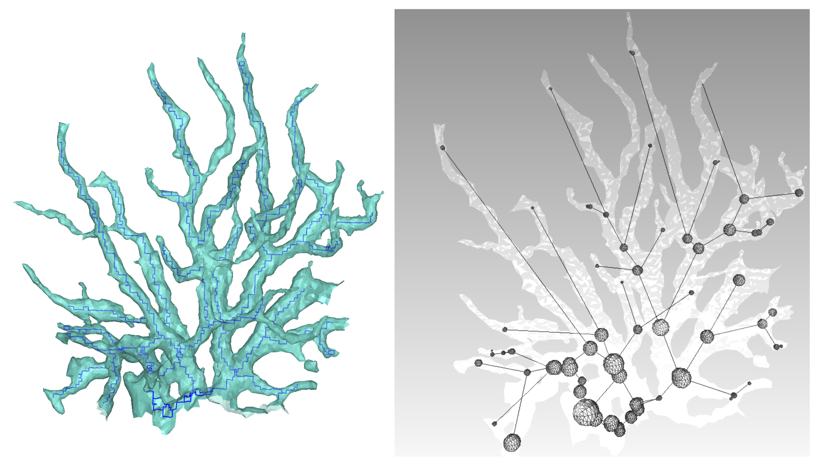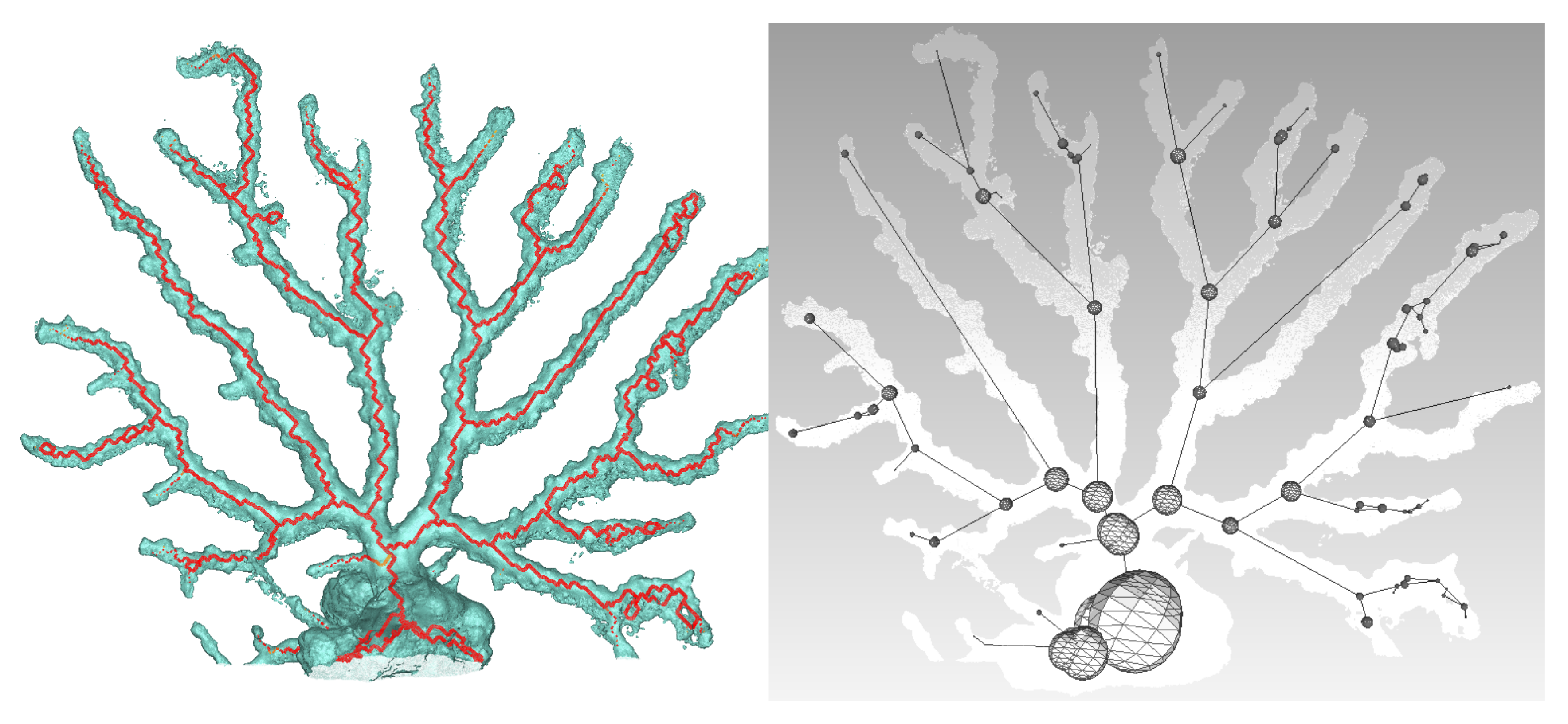Finally, thinning is performed while keeping the medial cells. Examples of resulting skeletons are shown in Figure 13 and Figure 14.

5.3.2. Extracting Relevant Information from the Skeleton

The next step is to build the tree that analytically describes the geometry of the polyps, from the set of lines of the skeleton. Each node of the tree corresponds to a junction between two branches. The distance between the nodes is also registered. Practically, from a starting point on the base, we iteratively read through the connected lines to this point. Each time three or more lines are connected to the same point, it is registered as a node and added to the tree. Once we have a structured representation of the skeleton, we can use it to extract new dimensional data. The first analysis that was performed was the estimation of the diameter of the branches. As branches are not perfect circles or ellipses and are also subject to noise, we decided that the best choice to evaluate the circumference would be the sphere that best fit the mesh centered on each node location. Practically, this is achieved in an iterative way, by starting from a small sphere and making it grow until it reaches the mesh. As this latter is not perfectly circular, a criterion is added to stop the algorithm when a certain amount of faces has been intersected.

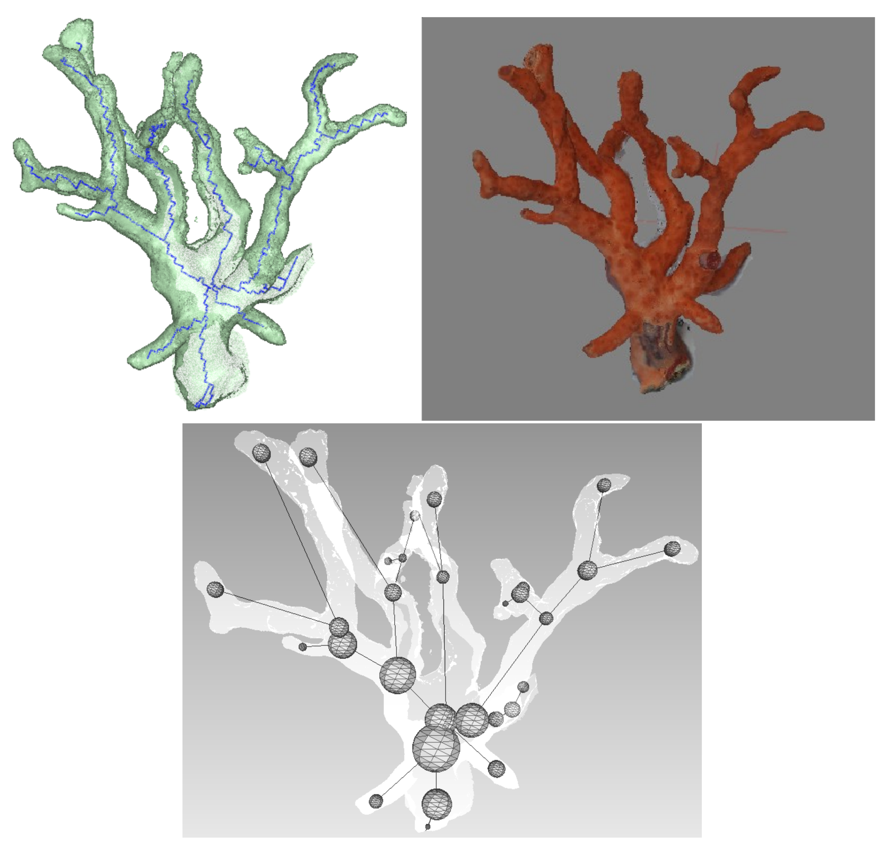
5.4. First Results

Using a Nikon D700, we took 118 photos of a dead coral colony placed on a desktop. Coded targets were positioned on the sides to scale the final model. After reconstruction, we obtained an accurate mesh containing about 450,000 faces. We first proceeded with the skeletonization as shown in Figure 15. Next, the graph describing the colony is built, as well as the spheres representing the local diameter at the node location. The result is visible in Figure 15. From these data, many extractions and interpretations are possible. For example, we decided to compute the total length of the branches and the approximate volume, using truncated cones between the arcs linking the spheres. Consequently, the resulting obtained length is $L=0.53$ m and the approximated volume is $V=1.28\times {10}^{-5}$ m${}^3$.

6. Plenoptic Approach

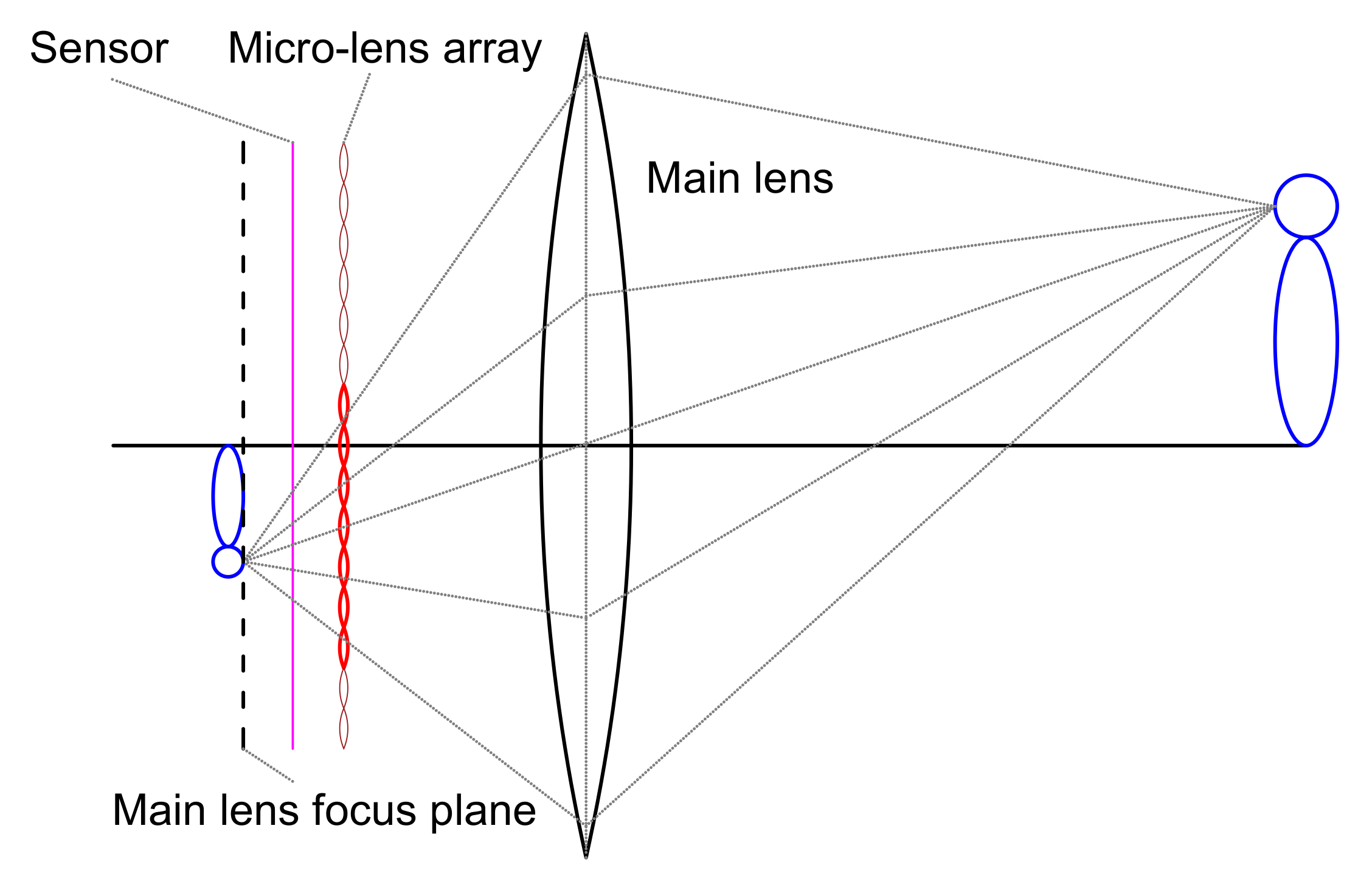
In traditional photogrammetry, it is necessary to completely scan the target area with many redundant photos taken from different points of view. This procedure is time-consuming and frustrating for large sites. Whereas many 3D reconstruction technologies are being developed for terrestrial sites relying mostly on active sensors such as laser scanners, solutions for underwater sites are much more limited. The idea of a plenoptic camera (also called light field camera) is to simulate a two-dimensional array of aligned tiny cameras. In practice, this can be achieved by placing an array of a micro-lenses between the image sensor and main lens as shown in Figure 16. This design allows the camera to capture the position and direction of each light beam in the image field, enabling the scene to be refocused or to obtain different views from a single lens image after image capture. The first demonstration dates from 2004 by a research team [62] at Stanford University.

In a plenoptic camera, each set of two close micro-lenses can be considered as a stereo pair if parts of the same scene appear in both acquired micro images. By applying a stereo matching method on the feature points of these micro images, it is possible to estimate a corresponding depth map. It is essential during image acquisition to respect a certain distance to the scene to remain within the working depth range. This working depth range can be enlarged but may affect the accuracy of the depth levels. In practice, the main lens focus should be set beyond the image sensor, in this case, each micro lens will produce a slightly different micro image for the object in regards to its neighbors. This allows the operator to have a depth estimation of the object. Recent advances in digital imaging resulted in the development and manufacturing of high-quality commercial plenoptic cameras. 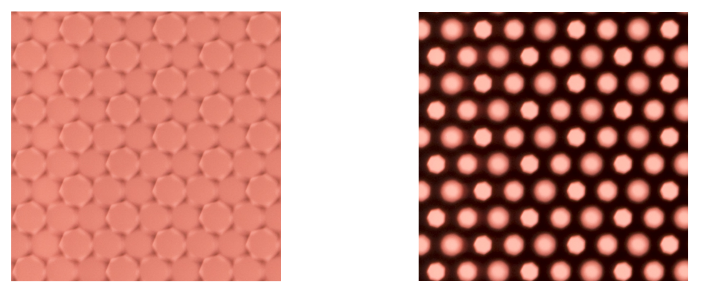Main manufacturers are Raytrix (Kiel, Germany) [63] and Lytro (Mountain View, CA, USA) [64]. While the latter concentrates on image refocusing and offline enhancement, the former focuses on 3D reconstruction and modeling, which is our interest here. The plenoptic camera used in this project is a modified version of a Nikon D800 by Raytrix. A layer that is composed of around 18,000 micro-lenses is placed in front of the 36.3 mega pixels CMOS (Complementary Metal Oxide Semi-conductor) original image sensor. The micro-lenses are of three types, which differ in their focal distance. This helps them to enlarge the working depth range, by combining three zones that correspond to each lens type; namely; near, middle and far range lenses. The projection size of micro-lens (micro images) can be controlled by changing the aperture of the camera. In our case, the maximum diameter of a micro image is approximately 38–45 pixels depending on the lens type. Figure 17 illustrates two examples of captured plenoptic images showing micro images taken at two different aperture settings.

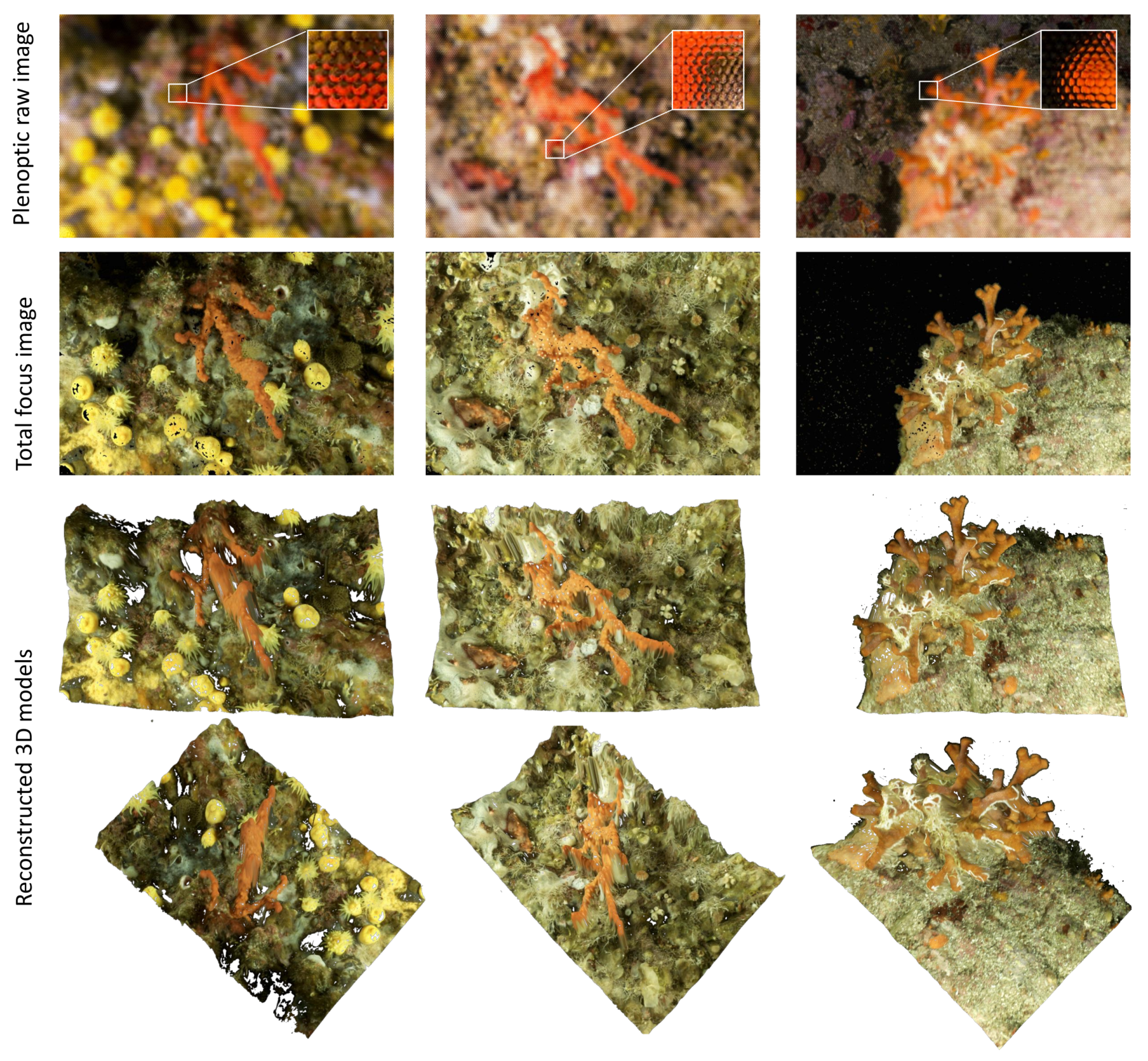
Our goal is to make this approach work in the marine environment so that only one shot is enough to obtain a properly scaled 3D model, which is a great advantage underwater, where diving time and battery capacity are limited. The procedure to work with a plenoptic camera is described in the following. Figure 18 shows examples plenoptic underwater images and reconstructed 3D models.

• Micro-lens Array (MLA) Calibration step: This step computes the camera’s intrinsic parameters, which include the position and the alignment of the MLA. The light field camera returns an uncalibrated raw image containing the pixels’ intensity values read by the sensor during shooting. Individual micro-lenses can be distinguished in the raw image. To localize the exact position of each the micro-lens in the raw image, a calibration image is taken using a white diffusive filter generating continuous illumination to highlight the edges and vignetting of each micro-lens as shown in Figure 17 (left). Using simple image processing techniques, it is possible to localize the exact position of each micro-lens, which corresponds to its optical center up to sub-pixel accuracy. In the same way, by taking another calibration image after changing the aperture of the camera so that the exterior edges of micro-lenses are touching (in Figure 17 (right)), we could use circle fitting to detect the outer edges of the micro-lenses with the help of the computed centers’ positions. Hence, for any new image without the filter, it is possible to easily extract the micro images. There is no need to perform the MLA calibration underwater. The location and the size of micro lenses do not change as soon as the aperture and the focus of the camera is fixed. Finally, a metric calibration must also be performed to convert from pixels to metric units. Here, the use of a calibration grid enables determining very accurately the internal geometry of the micro-lens array. The calibration results provide many parameters: intrinsic parameters, orientation of MLA, and tilt of the MLA in regards to the image sensor as well as distortion parameters.
• MLA Imaging: Each of these micro lenses capture a small fraction of the total image. These micro images can be synthesized to form the processed image in a focal plane. To do this, the depth (the distance from the object to the micro lens) must be taken for each pixel. For each point (x, y) in the object space, a set of micro lenses is selected that captures this point in their image plane. Then, the projection of this point (x, y) on the complete image plane by each micro lens is determined. The color value for the pixel in the full image plane is taken as the (weighted) average of the micro image values.
• Total focus processing: As different types of micro lenses are present with a different focus for each type throughout the MLA, each group of similar micro lenses is considered as a sub-array. An image with “full focus” or an image in which a large depth of field is maintained can be synthesized using several sub-arrays of different focal lengths to compute a sharp image over a large distance. For more details on the total focusing process, we refer to Perwass and Wietzke [65].
• Depth map computation: A brute force stereo points matching is performed among neighboring micro-lenses. The neighborhood is an input parameter that defines the maximum distance on the MLA between two neighboring micro-lenses. This process can be easily run in parallel. This is achieved using RxLive software that relies totally on the GPU. The total processing time does not exceed 400 milliseconds per image. Next, using the computed calibration parameters, each matched point is triangulated in 3D in order to obtain a sparse point cloud.
• Dense point cloud and surface reconstruction: In this step, all pixel data in the image are used to reconstruct the surface in 3D using iterative filling and bilateral filtering for smoother depth intervals.

7. Conclusions

This paper presents the results of more than 10 years collaboration between the computer science community and marine benthic biologists specialized in red coral. Through four kinds of the surveys, we developed different tools that can be applied to red coral study, our model species, to other species sharing the similar arborescents growth form, thus contributing to preserving it and protecting the marine coastal ecosystems.

These software programs will be available online (see http://perfect.medrecover.org) very soon.

Photogrammetry is the core of framework developed. Now widely used by many different scientific communities, the challenge is to extract relevant information from the reconstructed models.

First, we presented a graphical software enabling manual 3D measurements on couples of oriented photos, showing red coral colonies by a quadrat, which is used as scale tool and surface standard. The software provides reliable measurements (residuals generally lesser than 1 mm), for different estimations of the characteristics of colonies.

Next, we described a set of tools especially designed to study temporal changes. Monitoring the evolution of coral colonies over time and allowing for analyzing potential correlations between spatial distribution and relevant population parameters such as parental relationships and recruitment through genetic analysis in our case. The orthophotos of the studied sites are used to visualize the red coral colonies and then to compute true geodesic distances. Other tools, such as those used for orthophoto blending at different times, help advanced end users interpret the data.

Finally, the last survey presented was focused on archiving large red coral colonies and extracting relevant data from them. New approaches, including NPR representations and skeletonization of the 3D models, were developed in order to automatically compute morphological information, like volume and branch lengths, as well as obtaining simplified representations of these dense colonies. This density can prevent or make difficult observations by knowledgeable people.

Much work remains in order to increase the accuracy of estimated measurements of large coral colonies. Even if this study is focused on red coral, the different tools in this frame to better understand and characterize the functioning of benthic communities could be easily extended to other species with similar arborescent growth forms.

Beyond the geometrical and morphological survey and analysis we have done, we have started managing the huge quantity of data collected since the beginning of this collaboration. This data is mainly heterogeneous. We decided to use an ontology to manage all these data; indeed, LIS already have a lot of experience in managing photogrammetric data with ontologies in an archaeological context [66], and both the photogrammetric and the dimensional data of the coral colonies are already stored using Ontology Web Language (OWL) formalism. We are currently working on an extension of this approach in a 3D Information System dedicated to red coral survey based on photogrammetry survey and knowledge representation for spatial reasoning.