Regime Changes in Global Sea Surface Salinity Trend


1
Institut de Ciències del Mar - CSIC, Barcelona 08003, Spain
2
Integrated Statistics, Woods Hole 02543, MA, USA
3
Independent Research, West Tisbury 02575, MA, USA
*
Author to whom correspondence should be addressed.
J. Mar. Sci. Eng. 2017, 5(4), 57; https://doi.org/10.3390/jmse5040057
Submission received: 17 October 2017
/
Revised: 12 November 2017
/
Accepted: 17 November 2017
/
Published: 27 November 2017
(This article belongs to the Section Physical Oceanography)
Abstract
:Recent studies have shown significant sea surface salinity (SSS) changes at scales ranging from regional to global. In this study, we estimate global salinity means and trends using historical (1950–2014) SSS data from the UK Met Office Hadley Centre objectively analyzed monthly fields and recent data from the SMOS satellite (2010–2014). We separate the different components (regimes) of the global surface salinity by fitting a Gaussian Mixture Model to the data and using expectation–maximization to distinguish the means and trends of the data. The procedure uses a non-subjective method (Bayesian information criterion) to extract the optimal number of means and trends. The results show the presence of three separate regimes: Regime A (1950–1990) is characterized by small trend magnitudes; Regime B (1990–2009) exhibited enhanced trends; and Regime C (2009–2014) with significantly larger trend magnitudes. The salinity differences between regime means were around 0.01. The trend acceleration could be related to an enhanced global hydrological cycle or to a change in the sampling methodology. Understanding past SSS changes can provide insight into future climate evolution by complementing the knowledge acquired in recent decades from long-term temperature record analyses.
1. Introduction
Global sea surface salinity (SSS) is changing at scales ranging from regional to global [1,2]. Global salinity reflects the balance between surface freshwater flux (evaporation minus precipitation), terrestrial runoff, and mixing and advective processes in the ocean. Thus, changes in salinity are intrinsically connected to alterations in the global hydrological cycle and are expected to be a consequence of climate change [3]. The intensification of the global water cycle is expected to be occurring at a rate of 8% ° of surface warming [4] or around 20% considering the projected 2–3° of temperature increase over the next century. The mechanisms controlling the intensification of the water cycle have recently been evaluated [5,6].
Recently, Antonov et al. [1] and Boyer et al. [2] described a general change pattern with surface subtropical areas becoming saltier and high-latitude regions becoming fresher. Curry et al. [7] found increased salinity in the subtropical evaporation-dominated regions between 25° S and 35° N when they compared the time periods 1955–1969 and 1985–1999 for the entire Atlantic basin. Cravatte et al. [8] described a large freshening in the Pacific warm pool over the 1955–2003 period.
Hosoda et al. [9] analyzed global surface salinity comparing Argo float data for the period 2003–2007 with climatological 1960–1989 data from the 2005 World Ocean Database. The Argo data showed even lower salinities in fresher regions in recent times and higher salinities in areas of higher salinity magnitudes. They linked the changes in salinity to increased global hydrological cycle during the 30 years between their observations.
Friedman et al. [10] introduced a long-term dataset for the Atlantic Ocean and presented trends for several parts of the Atlantic. They related the trends and inter-decadal changes to climatic modes of variability such as the (NAO, Hurrell et al. [11]) and the Atlantic Multidecadal Oscillation (AMO, Kerr [12]).
Durack and Wijffels [13] (DW10 herein) analyzed data for the period 1950–2008 and found SSS increases in regions dominated by evaporation while freshening occurred in precipitation-dominated regions. They suggested the change was a consequence of an intensification of the global hydrological cycle. They also provided a comprehensive review of salinity changes in the literature. Using a linear fit for the 1950–2008 data, DW10 found that in a 50-year period, the subtropical gyres (evaporation dominated) exhibited net salinity increases from 0.20 in the eastern South Pacific to 0.45 in the subtropical North Atlantic. During the same period, the salinity decreased in the precipitation-dominated regions (for instance, under the Intertropical Convergence Zone (ITCZ)), with decreases ranging from −0.25 in the Equatorial Atlantic to −0.57 in the western Equatorial Pacific.
The SSS spatial pattern has been associated with the “rich get richer” mechanism for evaporation-precipitation [14]. In fact, the enhancement in hydrological cycle has been studied based on the changes in ocean salinity [4,15,16,17]. The intensification of the water cycle was larger over 1979–2010 than in earlier periods (1950–1978) related to the accelerated broad-scale warming [18].
The determination of a single SSS trend by DW10 highlighted significant challenges (e.g., data deficiencies in some regions and time periods), but it represented only a first step toward a characterization of the time evolution of global salinity. The results of recent analyses of other ocean parameters, such as water level [19,20], have demonstrated that changes in the ocean have been accelerated in recent times. In some regions, the rate of change of the water level time series exceeds even a quadratic fit over at least the last 50 years [19]. In fact, the role of salinity on water level changes has also been recently explored [21].
The question we are trying to address in this study is whether the SSS changes are due to: (1) a regime shift in which the SSS has moved from one equilibrium state to another (maybe even several regime shifts); (2) a constant SSS trend (no new equilibrium has been achieved); (3) a varying SSS trend (not only is SSS changing, but the rate of change varies); or (4) a combination of the above. The consequences of the SSS changes being associated with mean or trend changes have repercussions beyond the SSS evolution and affect the global water cycle [5,6,15]. Our goal is to isolate different regimes to provide understanding of potential future global cycle changes.
In this study, we separate the different regimes (components with substantially different characteristics) of the global SSS (1950–2014) by fitting Gaussian Mixture Models (GMM) with and without trends to the SSS data to characterize, not only the means, but also the trends. The GMMs are estimated using an expectation–maximization algorithm with the number of components determined non-subjectively by the Bayesian information criterion to extract the optimal number of means and trends. The method is chosen as a robust alternative to subjective trend estimation based on predetermined study periods. The long-term global SSS dataset from the UK Met Office Hadley Centre [22] is chosen as the reference data source. Recently available SMOS satellite data is used to complement the data from the period 2010–2014.
2. Data and Methods
2.1. Long-Term Global Salinity Data
The Met Office Hadley Centre provides global quality controlled ocean temperature and salinity profiles and monthly long-term objectively analyzed global fields with a one degree spatial resolution [22,23]. The most recent EN4 dataset (https://www.metoffice.gov.uk/hadobs/en4/) includes objectively analyzed fields formed from profile data with uncertainty estimates. The available data extend from the year 1900 to the present and there are separate files for each month. Good et al. [22] used a simple analysis correction [24] optimal interpolation methodology to analyze global historical observations that had been methodically quality controlled. The analysis fields were constructed by combining a background field (the analysis field of the previous month) with the quality controlled profiles from the month being analyzed.
2.2. SMOS Satellite Data
The recently available SMOS (Soil Moisture and Ocean Salinity) satellite [25,26] provides sea surface salinity data with sufficient spatial resolution () to characterize global [27] and regional (e.g., Amazon: [28]; North Atlantic SSS maximum: [29,30]; Gulf Stream: [31]; northern North Atlantic: [32]) features. Recently, SMOS data have been used to study salinity variability in the Atlantic [33], the signature of La Niña in the tropical Pacific Ocean [34] and even create surface temperature/salinity (T/S) diagrams [35]. The data is in constant evolution as more elaborate techniques are applied to the retrieval Olmedo et al. [36]. Level 3 (global maps) data were obtained from the CP34 distribution center at the SMOS Barcelona Expert Centre (http://tarod.cmima.csic.es) for the period 2010–2014. The temporal resolution of the objectively analyzed SMOS data is one month and the spatial resolution is . We averaged the data to one degree resolution to match the long-term dataset and reduce noisy signals.
The SMOS satellite data exhibited deficiencies near coastal areas and in high latitudes [29,32,37,38]. To prevent the introduction of bogus features, those data were removed from the analysis. The main areas affected were in high latitudes, in the proximity of continents, the Mediterranean, and in a large area of the western Pacific surrounding the Philippines and Japan.
2.3. Gaussian Mixture Models and Expectation-Maximization
A Gaussian Mixture Model (GMM) is a probabilistic model for which the probability density function is a combination of two or more Gaussian distributions. The expectation–maximization (EM) algorithm is an iterative procedure to find a maximum likelihood estimate (MLE) of the parameters of a GMM. In the past, the EM algorithm was used to separate the regimes of a spatial time series [39] and to find the best GMM describing the joint distribution of model and data in a model skill assessment scenario [40]. In previous studies, EM was used to estimate missing values for oceanographic datasets [41,42]. Aretxabaleta and Smith [28] introduced a measurement operator (H) and error (assuming the observations were unbiased with a Gaussian measurement error of known covariance, ), to provide a more general algorithm that could be used for missing data and interpolation problems.
In this implementation, we introduce the possibility of defining the GMM by both a mean and a linear temporal trend. After we have found the number of components (representing probability density functions), , component distributions (mean, trend, and covariance), , and their respective likelihoods, , we can conduct an empirical orthogonal function (EOF) analysis on the .
Let denote a set of time series with a linear measurement operator, , from a spatial basis on which we want to estimate the state at all time points, such that . We fit a mixture model to the data set, . For an component Gaussian mixture model, we have in general:
where is the spatial dimension of , is the probability of component distribution k, and , , and are the mean, trend, and covariance of the component distribution. is the determinant of the covariance.
The two steps of the EM iterative procedure are:
- Expectation step: For each time point, t, in the dataset, the expected value for component k of the likelihood function, , is calculated under the current estimate of the parameters (mean), (trend), and (covariance):Then, the likelihoods are normalized,
- Maximization step: The optimal parameters that maximize the current estimate given the data are calculated. Note that , , , and may all be maximized independently of each other since they appear in separate linear terms. The frequency of the k-th component distribution, , is computed and normalized,where is the length of the time series.
We enforced that the time series is an autoregressive process of order one (AR(1)) to avoid rapid switching between regimes. Thus, the salinity at time t depends linearly on the previous value, , where c is a constant, is the parameter of the AR(1) model and is white noise.
An EOF analysis can be conducted based on the component distributions covariances, . Using the eigenvectors of , we obtain a new set of orthogonal basis functions that are meaningful for times when . The EOF analysis can be considered independently during different regimes in a similar approach to Tipping and Bishop [43].
Our approach is related to the multivariate adaptive regression splines (MARS) method [44], as both automatically determine the number and timing of the separation between regimes (breakpoints or knots) based on the data. The main difference between the two approaches is that our method includes multiple spatial location (multiple time series) and the regime extraction is across the complete dataset.
2.4. Non-Subjective Choice of Number of Regimes: Bayesian Information Criterion
To determine the optimal number of components (regimes) in the GMM, we use the Bayesian Information Criterion (BIC, [40,45]). The BIC is an empirical approach that approximates the total probability (Bayes factor) of a probability distribution under some set data,
The penalty term preventing over-fitting, , for a GMM with components and n time series is , where of those are for the means of each distribution, another correspond to the trends, are for the parameters of the covariance matrix, and for the .
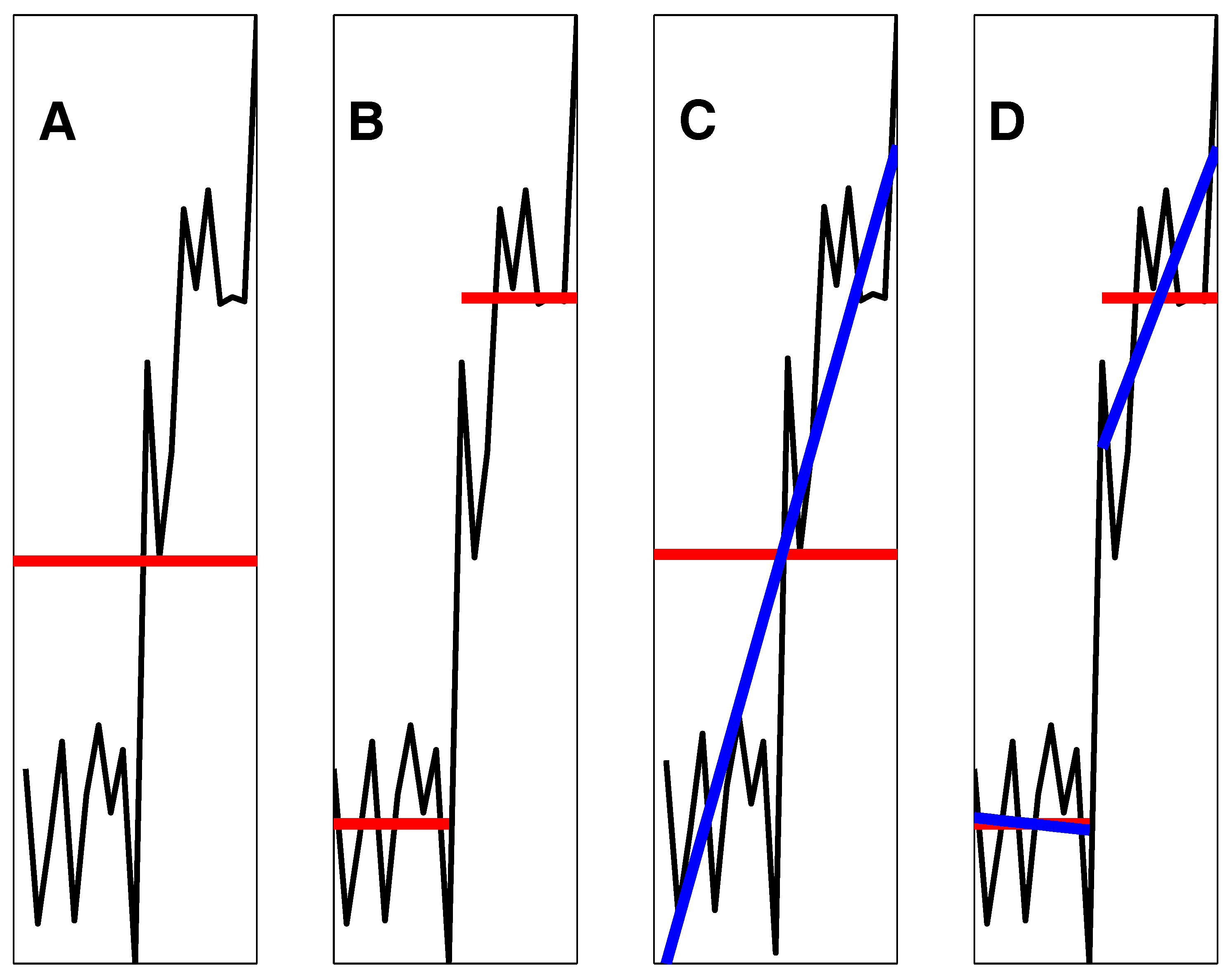
There are a number of potential combinations of means and trends (Figure 1) that can be fitted to any spatial time series. In the current application, the expectation–maximization (EM) algorithm is used to find the best GMM describing the data distribution. The method is run under several possible scenarios that separate regimes based on including only means, means and a global trend, and a combination of means and trends. The BIC approach penalizes excessive number of parameters with being adjusted depending on the inclusion/exclusion of trends. BIC is used twice in the current procedure: first, to choose the optimal number of components in a particular scenario (e.g., only means, combining means and trends), and second, to choose among the different scenarios.
3. Results
3.1. Comparison with DW10
The Hadley Centre EN4 surface salinity interpolated fields incorporated quality controlled observations in a similar manner as the database used by Durack and Wijffels [13] to create the DW10 surface fields. DW10 fields were reported for a 50 year period (nominally 1950–2000) to simplify comparisons, even though they used data from 1950 to 2008. To establish whether the datasets were sufficiently similar, we calculated the mean and trend for the same period as DW10 (1950–2008) using the interpolated data (Figure 2). The climatological mean surface salinity (Figure 2A) exhibits the same general structure and magnitude as the DW10 results. The standard deviation of the surface salinity (Figure 2B) highlights the increased variability associated with river discharge, the ITCZ, and intense meandering current systems like the Gulf Stream. As in the case of the mean, the 50 year linear surface salinity trend (Figure 2C) is also similar to the published fields with minimal differences. For instance, there is a slightly less negative trend in the Equatorial and North Atlantic and a larger positive trend in the Antarctic Circumpolar Current region in our results. Overall, the trend magnitude and spatial distribution for the 1950–2008 period are equivalent in both datasets. The main trend features include a predominantly positive trend in the Atlantic, southeastern Pacific, and Indian Ocean, and a predominantly negative trend in the north and western Pacific and along the Antarctic Circumpolar Current region.
3.2. Regime Separation Using Hadley Centre EN4 1950–2014 Fields
When the global SSS monthly data from the Hadley Centre EN4 were analyzed, the EM method distinguished three separate regimes. These regimes are characterized by different means, but also different trends (Figure 3 and Figure 4). The separation (breakpoint) between the first two regimes (Regime A and B) occurs in May 1990, while the separation between the second and third regimes (Regime B and C) was found to be March 2009.
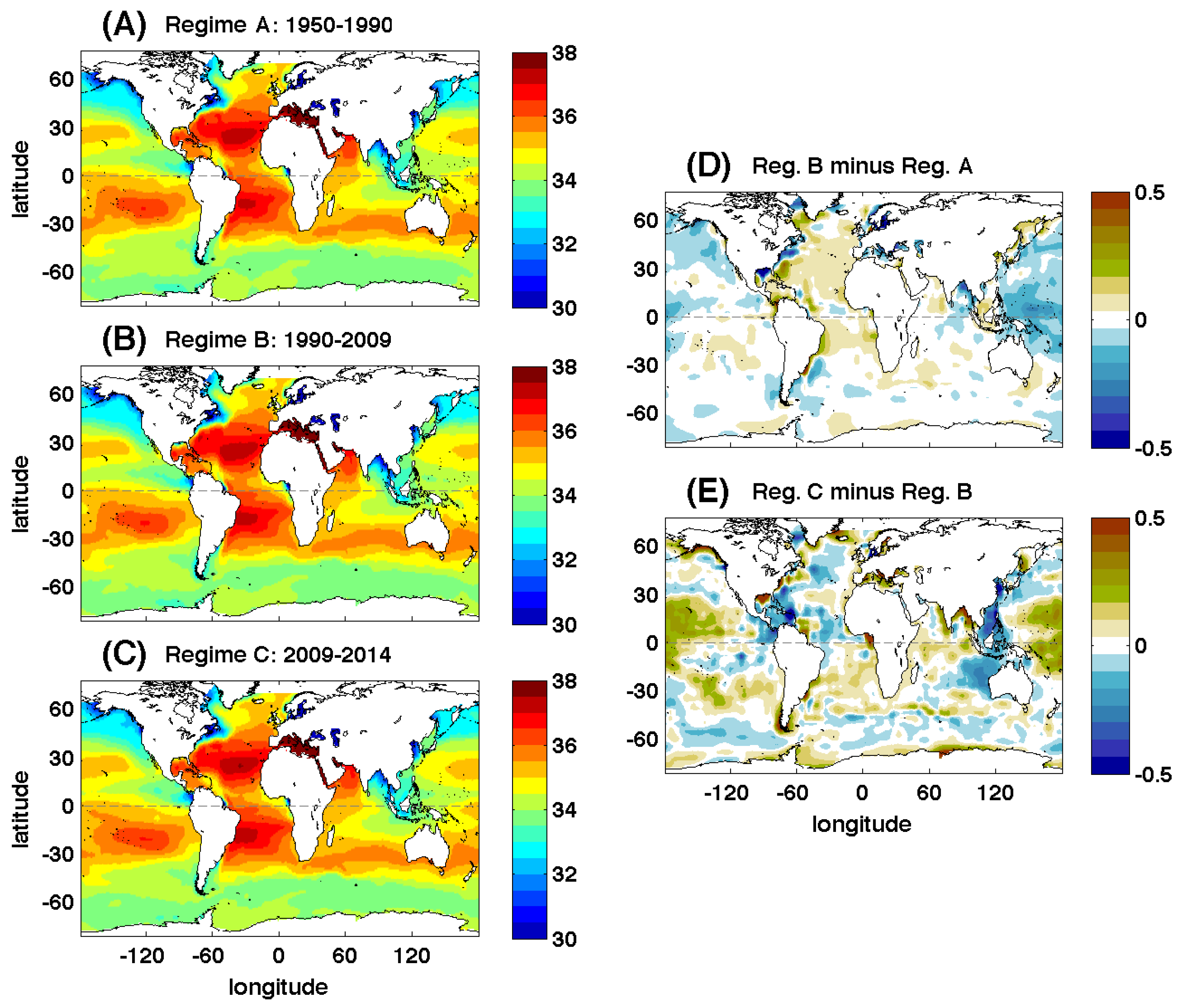
The global surface salinity means for the three regimes (Figure 3) exhibited the same general pattern with higher salinity in the subtropical gyres and lower values in the subpolar, polar regions, and under the ITCZ. The differences between regime means were on the order of 0.1 (0.099 rms difference between Regime A and B; and 0.15 between Regime B and C). The Regime B’s (1990–2009) average was saltier than Regime A’s (1950–1990) in most of the Atlantic Ocean except along the eastern U.S., in the central equatorial region, and south of 30° S. In contrast most of the Pacific (except for the southwest) was fresher in Regime B than A. The difference between the average salinities of Regime B (1990–2009) and Regime C (2009–2014) exhibited saltier values in the later period in most of the Pacific and South Atlantic, while a large part of the North Atlantic was fresher during Regime C.
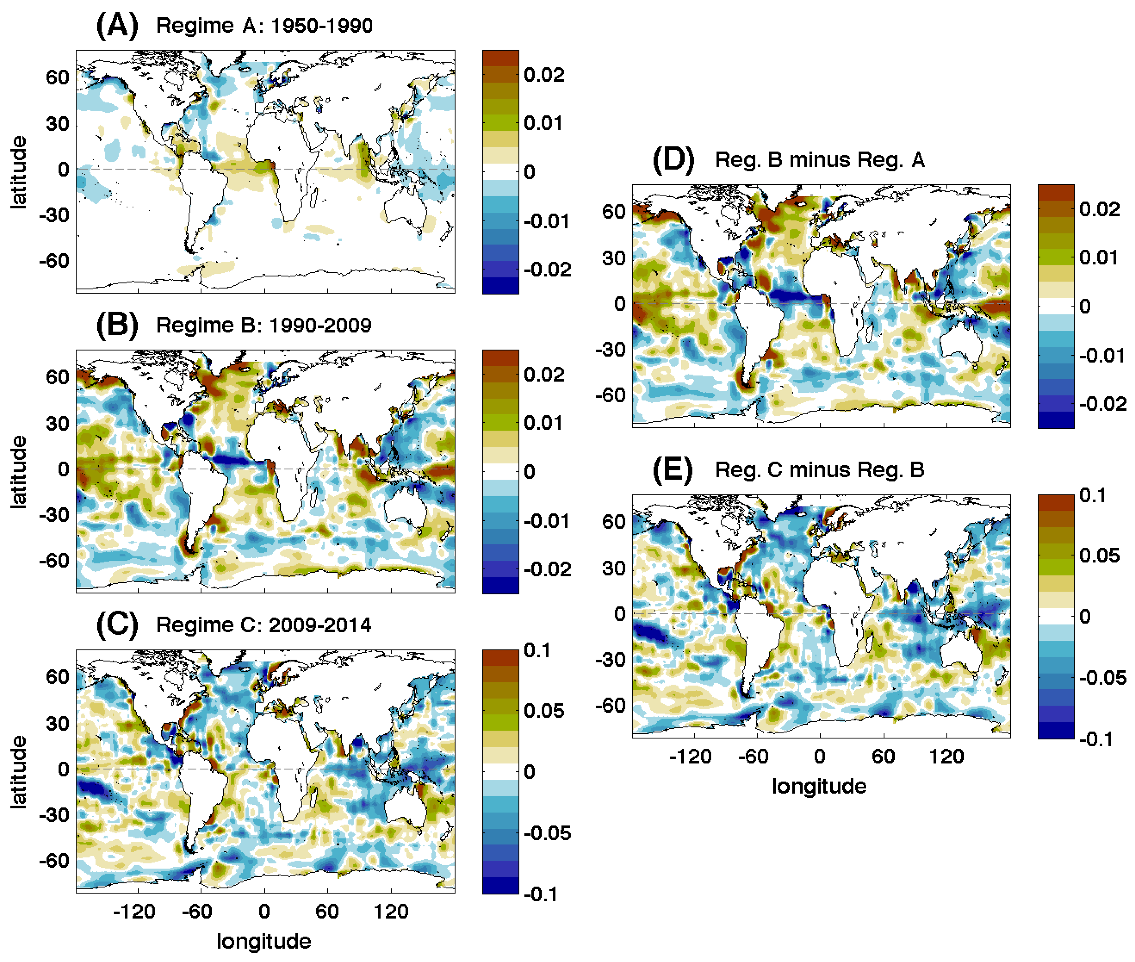
The trend for Regime A (1950–1990, Figure 4A) was consistent with the results obtained by DW10 (Durack and Wijffels [13] and Figure 2, note the different scale) and the references therein. The differences were a slightly larger positive trend in the Equatorial Atlantic and a lack of positive trend in the eastern Pacific. The trend for Regime B (1990–2009, Figure 4B) exhibited larger positive magnitudes in the North and South Atlantic than Regime A, a negative trend (∼ year) along the Equatorial Atlantic, negative trends in the areas of the Antarctic Circumpolar Current and positive trends (0.01–0.02 year) in most of the Pacific between 30° S and 30° N. The trend associated with Regime B exhibited enhanced magnitudes when compared to Regime A (positive trends were more positive and negative areas were more negative during Regime B). In both regimes the trends are consistent with an intensification of the global hydrological cycle [46,47]. The estimated trend during Regime C (2009–2014, Figure 4C) was much larger than in any of the two early regimes. The Regime C trend was negative in the majority of the North Atlantic (up to −0.04 year), eastern Indian Ocean (∼ year) and western (< year) and south Equatorial (∼ year) Pacific. Positive trends during Regime C were estimated along the western part of the Equatorial and South Atlantic (up to 0.06 year), the Pacific subtropical gyres (ranging 0.02–0.05 year) and the western Indian Ocean (∼ year).
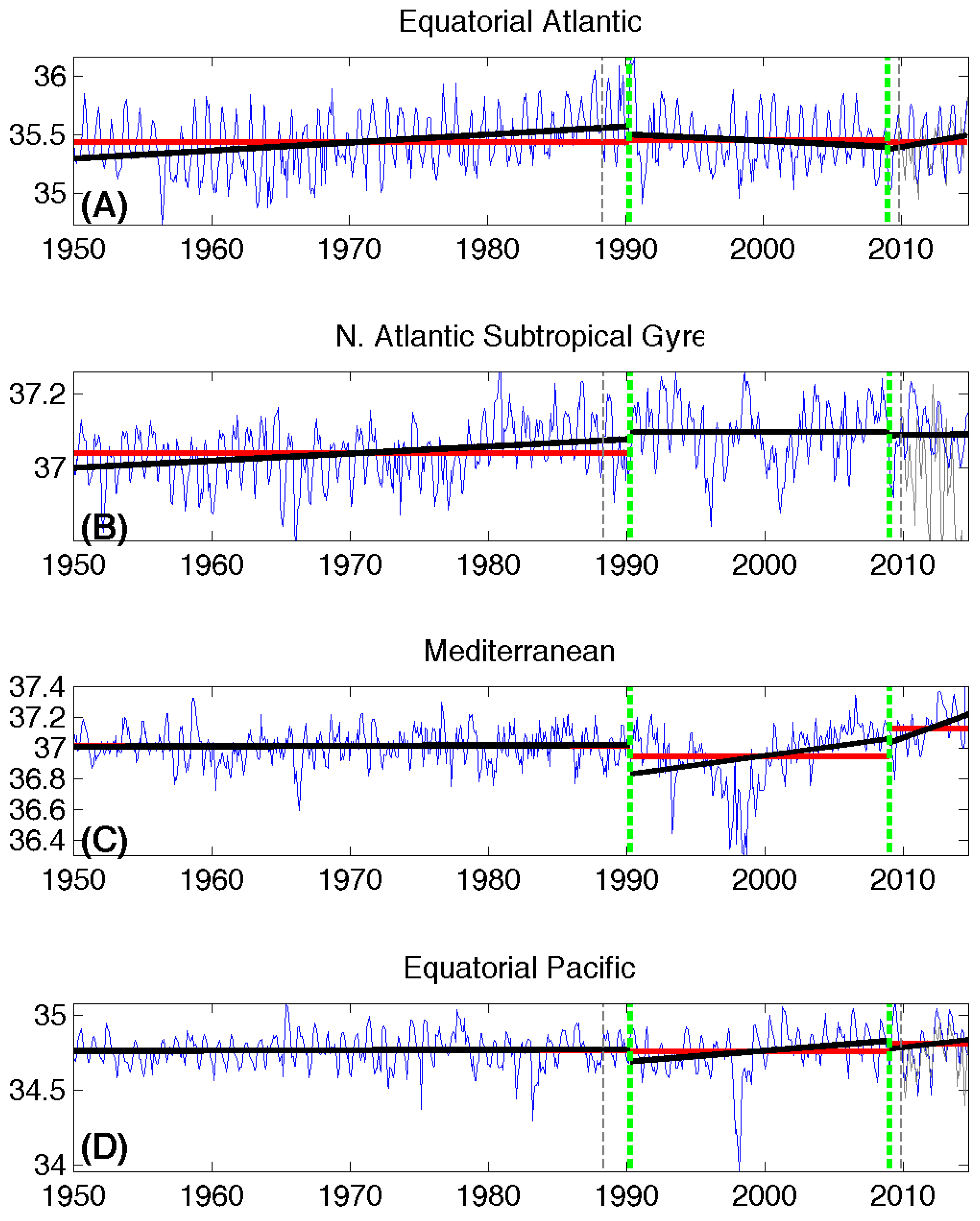
The salinity time evolution showed the changing temporal pattern during the full record and the potential distinction between regimes (Figure 5). For instance, the Equatorial Atlantic (Figure 5A, 5° S–5° N) showed a notable difference between the trends for the three regimes, while the difference between the average salinity of the three regimes was small. The North Atlantic Subtropical Gyre (Figure 5B, 15–30° N) in contrast exhibited noticeable differences in the trends, but especially in the means between the three regimes. Meanwhile, the most striking feature in the Mediterranean (Figure 5C) and in the Equatorial Pacific (Figure 5D, 5° S–5° N) was the sharp drop in salinity associated with El Niño events while the main difference between regimes was again in the magnitude of the trend. The largest trend acceleration between regimes was present in the Mediterranean (Figure 5C).
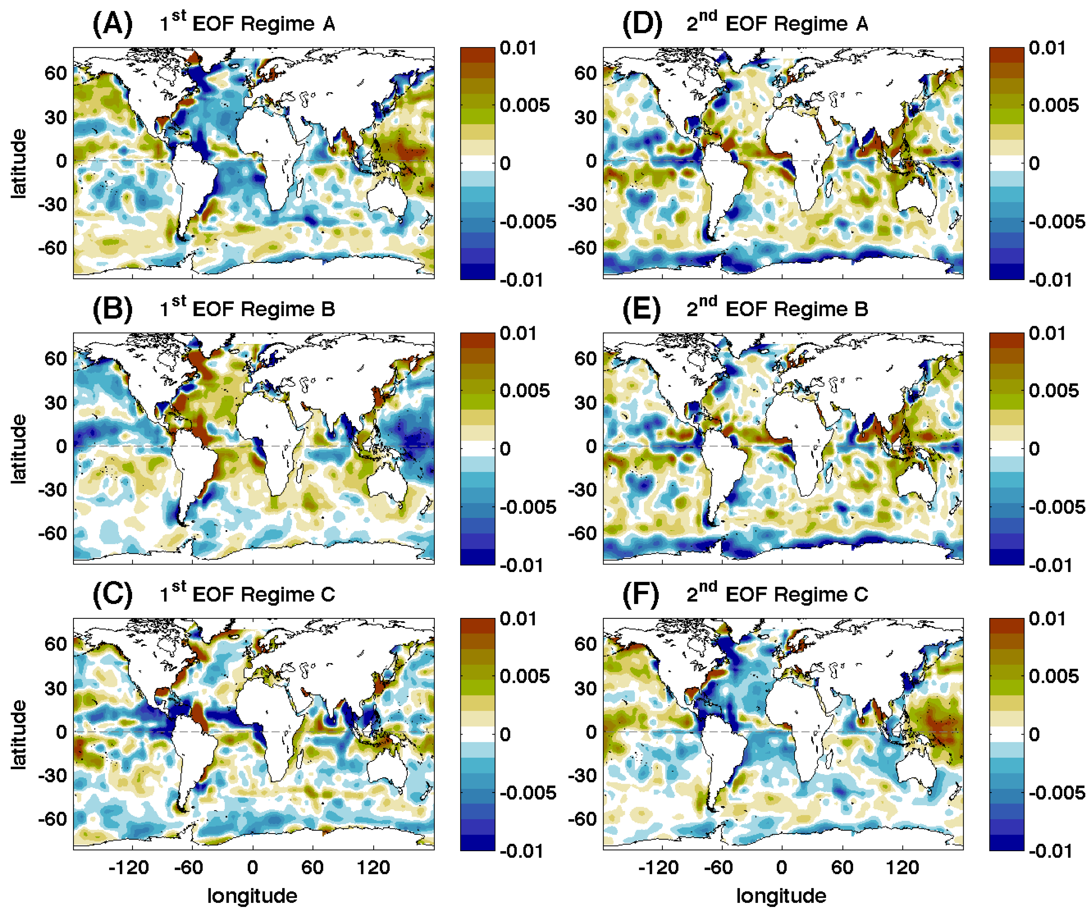
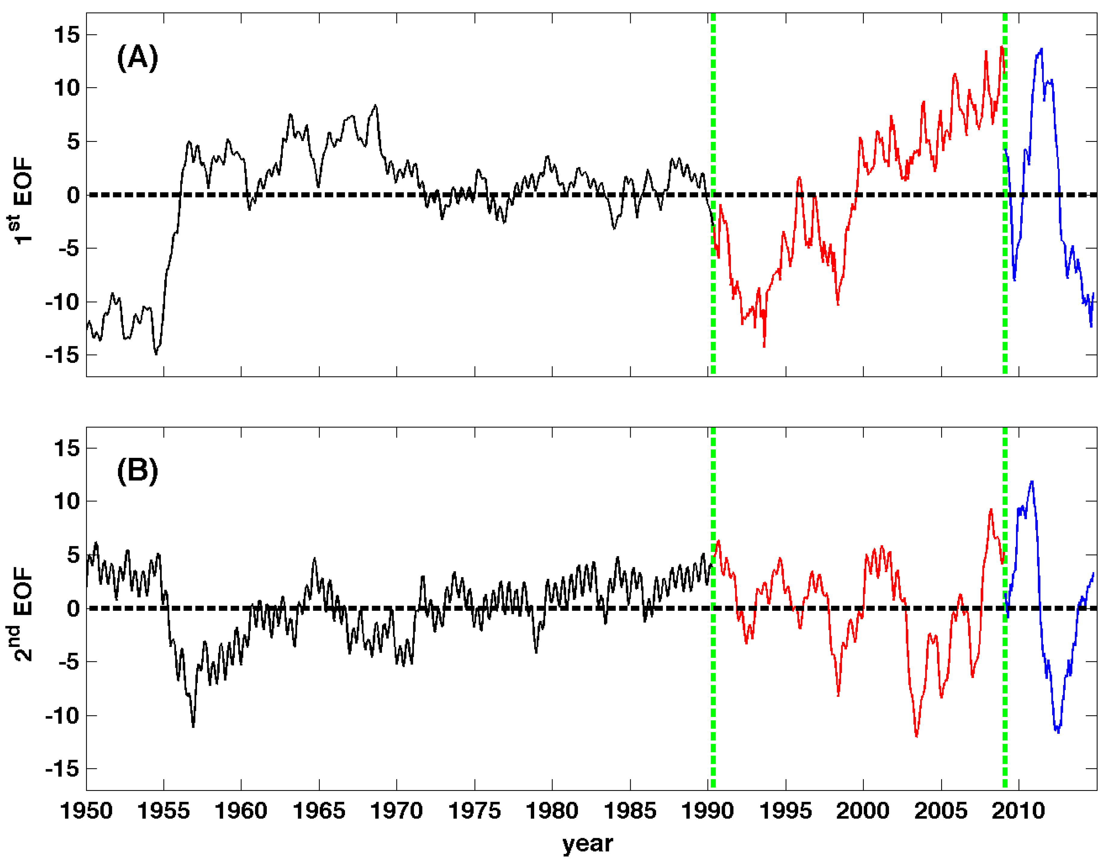
As described in Section 2.3, the EM algorithm also allowed for the separation of the modes of variability. The first EOF for Regimes A and B explained over 75% of the variance (79% and 77%, respectively) while only explaining 67% of the Regime C variance. Meanwhile, the second EOF explained 11%, 12% and 14% of the variance in each regime. The first EOF of Regime A was spatially consistent with Regime B, but its magnitude was smaller (Figure 6). The first EOF in the first two regimes suggested the Atlantic and southeastern Pacific were fluctuating in phase, while the western Pacific and most of the Southern Ocean were out of phase. The first EOF of Regime C exhibited a different spatial pattern and larger magnitude with the separation between basins being less apparent, with the main feature likely associated with the northern/southern migration and extent of the ITCZ. The second EOF for the first two regimes was quite similar with positive values in most areas except the Antarctic and Equatorial Pacific oceans. Meanwhile, the second EOF of Regime C was mostly consistent with the Pacific and Atlantic oceans being out of phase. The time series of the first EOF (Figure 7A) showed larger short-term fluctuations for Regime B and Regime C, with Regime B exhibiting a trend in time. There was an apparent relationship between the second EOF for Regime B (Figure 7B) and the ENSO cycle (1998, 2003, 2005 peaks), while no clear relation appeared to be present for Regime A or C.
3.3. Regime Separation with Updated SMOS Fields 2010–2014
The recent availability of global surface salinity fields from satellites (SMOS and Aquarius) provided the possibility of using alternative data that were not included as part of the Good et al. [22] dataset. The goal was to analyze the robustness of the regime separation by replacing the recent (2010–2014) fields with satellite-derived products.
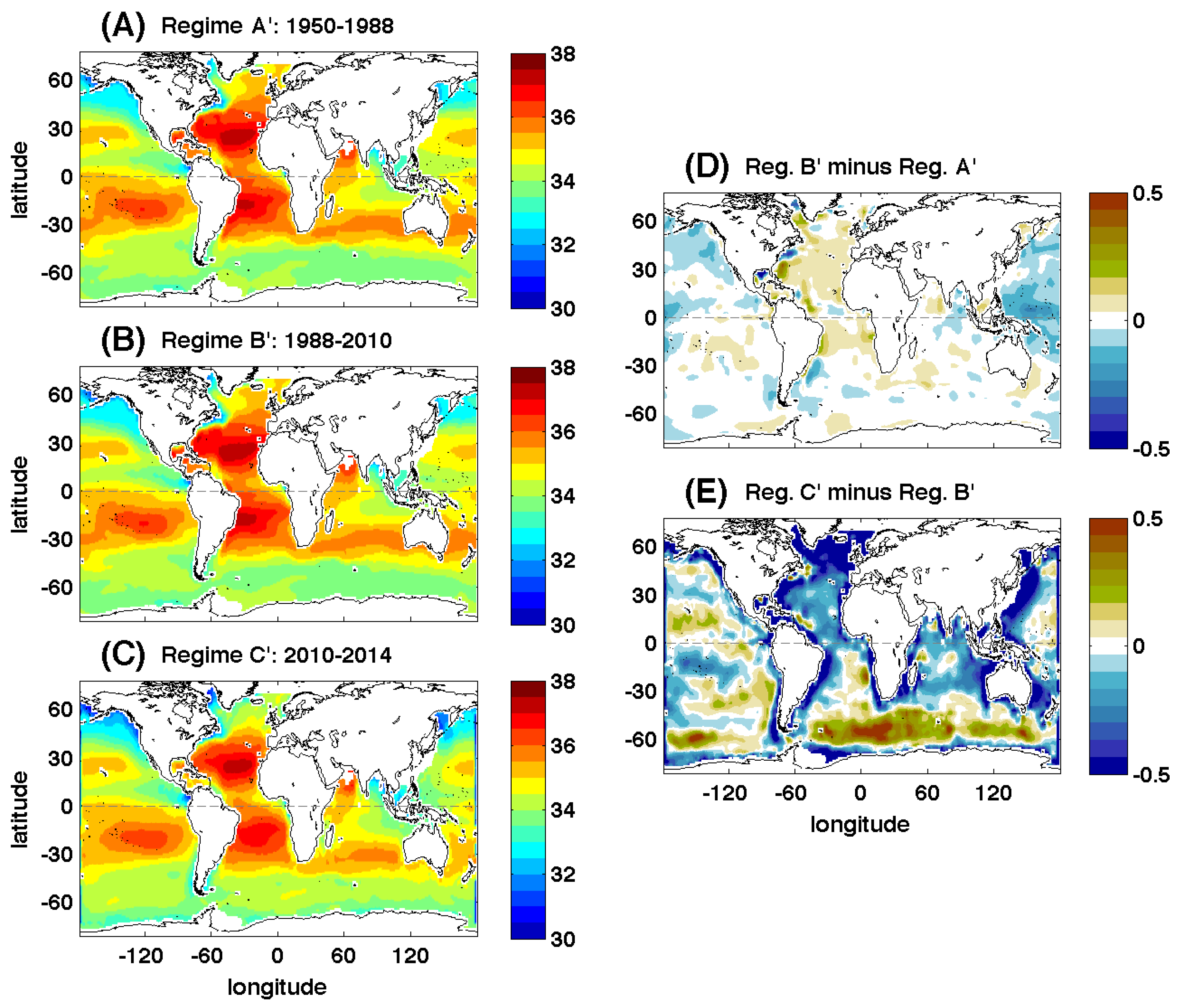
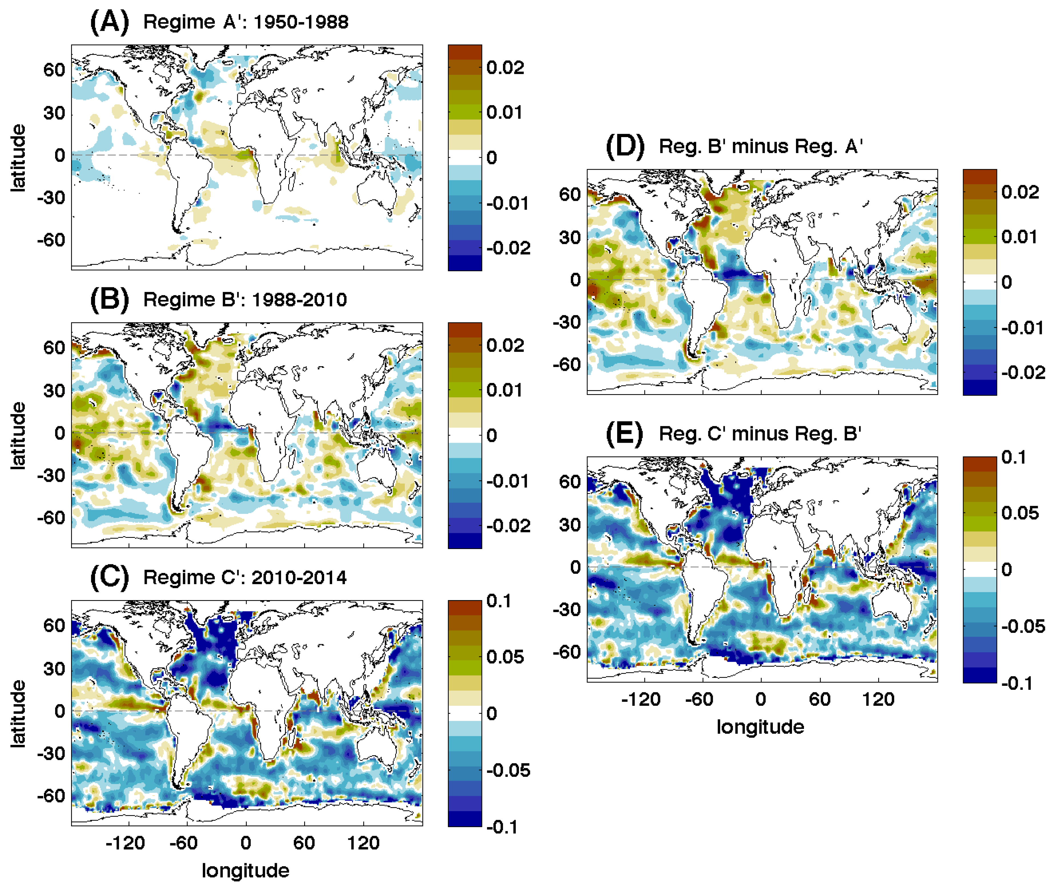
The inclusion of the available five years of SMOS data in the analysis in substitution of the EN4 data for 2010–2014 slightly altered the EM separation results (Figure 8 and Figure 9). The EM method also distinguished three separate regimes (A’, B’, and C’) with different means and trends. The breakpoint between Regime A’ and B’ was in July 1988 and between Regime B’ and C’ in January 2010. The difference in the separation (breakpoint) dates between the early regimes was expected as the merged dataset did not include several areas (proximity to coastal areas, Mediterranean Sea, high latitude) that were present in the original EN4 dataset.
The means and differences of the two first regimes (Figure 8A,B,D) were equivalent to the results for the complete EN4 dataset (Figure 3). The average salinity for Regime C’ (Figure 8C) exhibited significant differences from both the Regime B’ mean and also from the third regime of the original dataset (Regime C, 2009–2014). The mean salinity during Regime C’ was fresher in the North (up to −0.5) and Equatorial Atlantic, the Indian and Western Pacific Oceans, while being saltier in most of the Southern Ocean and in large areas of the Pacific Ocean.
As was the case with the means, the trends of the two first regimes (A’ and B’) of the combined time series (Figure 9A,B) were equivalent to the trends extracted from the original dataset (Figure 4) for Regimes A and B. The trend for Regime C’ (2010–2014, Figure 9C) differed in magnitude and spatial structure from the trend for Regime C of the original EN4 dataset (2009–2014, Figure 4C). The Regime C’ trend was positive in the Equatorial Pacific and Atlantic while having a negative trend in most of the rest of the oceans with large negative values especially in the North Atlantic. The trend for Regime C’ was likely the effect of changes in the processing methodology for global SMOS data [37,38].
4. Discussion
The two early regimes (A: 1950–1990; and B: 1990–2009) are consistent with the idea of salinity change acceleration caused by enhanced hydrological cycle. The most recent period (2009–2014) might be too short to be considered a robust regime change. The water cycle has been shown to be farther increased in the period 1979–2010 due to accelerated warming [18]. Durack et al. [4] analyzed modeling scenarios for the 20th century (Coupled Model Intercomparison Project Phase 3, CMIP3, [48]) that are consistent with not only a linear increase in hydrological cycle magnitude but also an acceleration of the intensification. The CMIP3 scenarios showed the expected intensification of existing patterns of global mean E-P (“rich get richer” mechanism) and the resulting salinity pattern amplification. The changes calculated from ocean observations were consistent with the scenario simulations but with a slightly larger effect of global surface warming on salinity pattern amplification [4]. The spatial patterns in the CMIP3 climate simulations matched the observed salinity pattern in many areas and were consistent with the spatial structure in the present study.
The described salinity change acceleration is likely the result of global hydrological cycle intensification as was suggested by Hosoda et al. [9] and Durack and Wijffels [13]. The areas of enhanced precipitation and evaporation [46,47] correspond with the largest magnitude changes in salinity [14]. The changing trend in salinity will further enhance the hydrological cycle intensification described in Durack et al. [4] with modifications larger than the proposed 20% in the next century.
While the study focuses on the near-surface salinity, the vertical extent of the changes can be much larger. Boyer et al. [2] described significant changes with varying vertical range depending on the basin (500 m in the Pacific, 1000 m in the Indian, and 3000 m in the Atlantic Ocean). The vertical extent of the increased salinity seems to be larger than the extent in areas of freshening. The relationship between salinity and density complicates the basic hypothesis of salinity changes being primarily surface forced [13,17]. The combined temperature and salinity changes need to be understood to explain the observed changes, especially in the interior of the water column.
The presence of embedded climate variability cycles like ENSO [49], NAO and AMO [10] can alter the values of trend provided for each regime, but it will not alter the general pattern of changes. Careful consideration should be provided to the effect of decadal variability associated with climate modes when shorter regimes are considered (e.g., the most recent period).
As the sampling methodology and number of observations have evolved in time, the trend acceleration in recent times might not be a completely realistic feature. Skliris et al. [18] suggested that while water cycle intensification was consistent with the warming trend, it also matched the improved salinity sampling. The availability of extensive field cruises in the last few decades and especially the development of the Argo network of profiling drifters over the last 15 years have altered the quantity, quality and spatial coverage of observations. The Argo network was established in 2001 and since 2006 has maintained more than 3000 active floats resulting in a nominal horizontal sampling of around 300 km. The result is a more intense sampling of the global salinity in recent years and also a switch from cruise-dependent locally intense sampling to more automatic sampling by profilers, floats and gliders. The changing trends can be the result of the changing measurement methodologies and spatial and temporal resolutions. Proper quality control of recent measurements will minimize this effect.
High quality global surface salinity fields that consider multiple instrument sources, measurement error and instrument quality are currently being developed [27,36,50]. Careful validation of any new data is fundamental for the success of the EM method or any other procedure to characterize the means and trends of long-term datasets.
5. Summary and Conclusions
In this study, we have analyzed global salinity datasets to identify a series of regimes characterized by fluctuations around a changing average and temporal tendency (trend). The separation between regimes is achieved through the analysis of global features fitting a Gaussian Mixture Model to the data and using an expectation–maximization algorithm to determine the parameters that best describe the spatial salinity time series. The datasets used include global monthly fields from 1950 to 2014 with a global resolution of one degree.
The EM method allows for the separation of regimes based on their averages and trends assuming the spatial time series is a combination of Gaussians (GMM). The method uses Bayesian information criterion to choose the appropriate number of means/trends by penalizing excessive overfitting. The resulting fit represents the maximum likelihood estimate (MLE) chosen using a non-arbitrary separation.
The method distinguished between three regimes characterized by distinct mean and trend. Regime A (1950–1990) was similar to the long-term average and trend described in several recent studies [2,8,13]. Regime B (1990–2009) was characterized by a similar average with slightly fresher Pacific and saltier Atlantic, but with larger trend magnitudes that are consistent with an enhanced global hydrological cycle. Regime C (2009–2014) showed a further intensification of the trend magnitudes with generally more positive trends in large areas of the Southern Hemisphere and negative trends in the North Atlantic, eastern Indian and western Pacific oceans. When the last 5 years of data (2010–2014) were replaced by salinity measured by the SMOS satellite, the separation between regimes, while not completely equal, exhibited similar spatial and temporal features demonstrating the robustness of the method.
A future goal is to use long-term satellite data from SMOS and Aquarius to determine if the estimated means and trends are well-constrained. The issue with long-term data analysis is that the trend estimates can change, as new data become available. The presented estimates can be relevant to the period studied, but trend projection into the future should be avoided. Our specific goal was to characterize SSS regimes to provide guidance on potential future global cycle changes without the characterization representing a forecast of future conditions. The combination of densely-distributed in situ observations (Argo profilers) and remotely-sensed satellite data (e.g., Droghei et al. [51]) will help constrain the variability in the evolving global salinity field.
Acknowledgments
This study has been funded by the Spanish Ministry of Economy through the National R1D Plan by means of MIDAS-7 Project AYA2012˘39356−C05−03. The historical time series was obtained from the UK Met Office Hadley Centre (http://www.metoffice.gov.uk/hadobs/en4/). The SMOS data were produced by the Barcelona Expert Centre (www.smos-bec.icm.csic.es), a joint initiative of the Spanish Research Council (CSIC) and the Technical University of Catalonia (UPC), mainly funded by the Spanish National Program on Space. The authors thank the efforts of the entire SMOS-BEC to produce improved SSS products while being an outstanding working environment. The authors thank Ray W. Schmitt (Woods Hole Oceanographic Institution) for his support and comments on the manuscript. A.L. Aretxabaleta was supported by a Juan de la Cierva grant from the Spanish Government during the early stages of the study. K.W. Smith was supported by his wages at Lowe Energy Design.
Author Contributions
A.L.A. conducted the analysis and wrote most of the article. K.W.S. developed and implemented the methodology and provided guidance with the data analysis. T.S.K. provided comments on the later stages of the article.
Conflicts of Interest
The authors declare no conflict of interest.
References
- Antonov, J.I.; Levitus, S.; Boyer, T.P. Steric sea level variations during 1957–1994: Importance of salinity. J. Geophys. Res. 2002, 107. [Google Scholar] [CrossRef]
- Boyer, T.P.; Levitus, S.; Antonov, J.I.; Locarnini, R.A.; Garcia, H.E. Linear trends in salinity for the World Ocean, 1955–1998. Geophys. Res. Lett. 2005, 32. [Google Scholar] [CrossRef]
- Held, I.M.; Soden, B.J. Robust responses of the hydrological cycle to global warming. J. Clim. 2006, 19, 5686–5699. [Google Scholar]
- Durack, P.J.; Wijffels, S.E.; Matear, R.J. Ocean Salinities Reveal Strong Global Water Cycle Intensification During 1950 to 2000. Science 2012, 336, 455–458. [Google Scholar] [CrossRef] [PubMed]
- Ponte, R.; Vinogradova, N. An assessment of basic processes controlling mean surface salinity over the global ocean. Geophys. Res. Lett. 2016, 43, 7052–7058. [Google Scholar] [CrossRef]
- Vinogradova, N.T.; Ponte, R.M. In Search of Fingerprints of the Recent Intensification of the Ocean Water Cycle. J. Clim. 2017, 30, 5513–5528. [Google Scholar] [CrossRef]
- Curry, R.; Dickson, R.R.; Yashayaev, I. A change in the fresh-water balance of the Atlantic Ocean over the past four decades. Nature 2003, 426, 826–829. [Google Scholar] [CrossRef] [PubMed]
- Cravatte, S.; Delcroix, T.; Zhang, D.; McPhaden, M.; Leloup, J. Observed freshening and warming of the western Pacific warm pool. Clim. Dyn. 2009, 33, 565–589. [Google Scholar] [CrossRef]
- Hosoda, S.; Sugo, T.; Shikama, N.; Mizuno, K. Global surface layer salinity change detected by Argo and its implication for hydrological cycle intensification. J. Oceanogr. 2009, 65, 579–586. [Google Scholar] [CrossRef]
- Friedman, A.R.; Reverdin, G.; Khodri, M.; Gastineau, G. A new record of Atlantic sea surface salinity from 1896 to 2013 reveals the signatures of climate variability and long-term trends. Geophys. Res. Lett. 2017, 44, 1866–1876. [Google Scholar] [CrossRef]
- Hurrell, J.W.; Kushnir, Y.; Ottersen, G.; Visbeck, M. An overview of the North Atlantic oscillation. In The North Atlantic Oscillation: Climatic Significance and Environmental Impact; Wiley Online Library: Hoboken, NJ, USA, 2003; pp. 1–35. [Google Scholar]
- Kerr, R.A. A North Atlantic climate pacemaker for the centuries. Science 2000, 288, 1984–1985. [Google Scholar] [CrossRef] [PubMed]
- Durack, P.J.; Wijffels, S.E. Fifty-year trends in global ocean salinities and their relationship to broad-scale warming. J. Clim. 2010, 23, 4342–4362. [Google Scholar] [CrossRef]
- Chou, C.; Neelin, J.D.; Chen, C.A.; Tu, J.Y. Evaluating the “rich-get-richer” mechanism in tropical precipitation change under global warming. J. Clim. 2009, 22, 1982–2005. [Google Scholar] [CrossRef]
- Schmitt, R.W. Salinity and the Global Water Cycle. Oceanography 2008, 21, 12. [Google Scholar] [CrossRef]
- Helm, K.P.; Bindoff, N.L.; Church, J.A. Changes in the global hydrological-cycle inferred from ocean salinity. Geophys. Res. Lett. 2010, 37. [Google Scholar] [CrossRef]
- Durack, P.J. Ocean salinity and the global water cycle. Oceanography 2015, 28, 20–31. [Google Scholar] [CrossRef]
- Skliris, N.; Marsh, R.; Josey, S.A.; Good, S.A.; Liu, C.; Allan, R.P. Salinity changes in the World Ocean since 1950 in relation to changing surface freshwater fluxes. Clim. Dyn. 2014, 43, 709–736. [Google Scholar] [CrossRef]
- Church, J.A.; White, N.J. A 20th century acceleration in global sea-level rise. Geophys. Res. Lett. 2006, 33. [Google Scholar] [CrossRef]
- Ezer, T. Sea level rise, spatially uneven and temporally unsteady: Why the US East Coast, the global tide gauge record, and the global altimeter data show different trends. Geophys. Res. Lett. 2013, 40, 5439–5444. [Google Scholar] [CrossRef]
- Durack, P.J.; Wijffels, S.E.; Gleckler, P.J. Long-term sea-level change revisited: The role of salinity. Environ. Res. Lett. 2014, 9, 114017. [Google Scholar] [CrossRef]
- Good, S.A.; Martin, M.J.; Rayner, N.A. EN4: Quality controlled ocean temperature and salinity profiles and monthly objective analyses with uncertainty estimates. J. Geophys. Res. Oceans 2013, 118, 6704–6716. [Google Scholar] [CrossRef]
- Ingleby, B.; Huddleston, M. Quality control of ocean temperature and salinity profiles—Historical and real-time data. J. Mar. Syst. 2007, 65, 158–175. [Google Scholar] [CrossRef]
- Lorenc, A.; Bell, R.; Macpherson, B. The Meteorological Office analysis correction data assimilation scheme. Q. J. R. Meteorol. Soc. 1991, 117, 59–89. [Google Scholar] [CrossRef]
- Font, J.; Camps, A.; Borges, A.; Martín-Neira, M.; Boutin, J.; Reul, N.; Kerr, Y.; Hahne, A.; Mecklenburg, S. SMOS: The Challenging Sea Surface Salinity Measurement From Space. Proc. IEEE 2010, 98, 649–665. [Google Scholar] [CrossRef] [Green Version]
- Font, J.; Ballabrera-Poy, J.; Camps, A.; Corbella, I.; Duffo, N.; Duran, I.; Emelianov, M.; Enrique, L.; Fernández, P.; Gabarró, C.; et al. A new space technology for ocean observation: The SMOS mission. Sci. Mar. 2012, 76, 249–259. [Google Scholar]
- Xie, P.; Boyer, T.; Bayler, E.; Xue, Y.; Byrne, D.; Reagan, J.; Locarnini, R.; Sun, F.; Joyce, R.; Kumar, A. An in situ-satellite blended analysis of global sea surface salinity. J. Geophys. Res. Oceans 2014, 119, 6140–6160. [Google Scholar] [CrossRef]
- Aretxabaleta, A.L.; Smith, K.W. Multi-regime non-Gaussian data filling for incomplete ocean datasets. J. Mar. Syst. 2013, 119, 11–18. [Google Scholar] [CrossRef]
- Hernandez, O.; Boutin, J.; Kolodziejczyk, N.; Reverdin, G.; Martin, N.; Gaillard, F.; Reul, N.; Vergely, J. SMOS salinity in the subtropical north Atlantic salinity maximum: 1. Comparison with Aquarius and in situ salinity. J. Geophys. Res. 2014, 119, 8878–8896. [Google Scholar] [CrossRef]
- Kolodziejczyk, N.; Hernandez, O.; Boutin, J.; Reverdin, G. SMOS salinity in the subtropical North Atlantic salinity maximum: 2. Two-dimensional horizontal thermohaline variability. J. Geophys. Res. Oceans 2015, 120. [Google Scholar] [CrossRef]
- Reul, N.; Chapron, B.; Lee, T.; Donlon, C.; Boutin, J.; Alory, G. Sea surface salinity structure of the meandering Gulf Stream revealed by SMOS sensor. Geophys. Res. Lett. 2014, 41, 3141–3148. [Google Scholar] [CrossRef]
- Köhler, J.; Sena Martins, M.; Serra, N.; Stammer, D. Quality assessment of spaceborne sea surface salinity observations over the northern North Atlantic. J. Geophys. Res. Oceans 2015, 120, 94–112. [Google Scholar] [CrossRef] [Green Version]
- Tzortzi, E.; Josey, S.A.; Srokosz, M.; Gommenginger, C. Tropical Atlantic salinity variability: New insights from SMOS. Geophys. Res. Lett. 2013, 40, 2143–2147. [Google Scholar] [CrossRef]
- Hasson, A.; Delcroix, T.; Boutin, J.; Dussin, R.; Ballabrera-Poy, J. Analyzing the 2010Ð2011 La Niña signature in the tropical Pacific sea surface salinity using in situ data, SMOS observations, and a numerical simulation. J. Geophys. Res. 2014, 119, 3855–3867. [Google Scholar] [CrossRef]
- Sabia, R.; Klockmann, M.; Fernandez-Prieto, D.; Donlon, C. A first estimation of SMOS-based ocean surface T-S diagrams. J. Geophys. Res. Oceans 2014, 119, 7357–7371. [Google Scholar] [CrossRef]
- Olmedo, E.; Martínez, J.; Turiel, A.; Ballabrera-Poy, J.; Portabella, M. Debiased non-Bayesian retrieval: A novel approach to SMOS Sea Surface Salinity. Remote Sens. Environ. 2017, 193, 103–126. [Google Scholar] [CrossRef]
- Guimbard, S.; Gourrion, J.; Portabella, M.; Turiel, A.; Gabarro, C.; Font, J. SMOS semi-empirical ocean forward model adjustment. IEEE T. Geosci. Remote 2012, 50, 1676–1687. [Google Scholar] [CrossRef]
- Yin, X.; Boutin, J.; Martin, N.; Spurgeon, P.; Vergely, J.L.; Gaillard, F. Errors in SMOS sea surface salinity and their dependency on a priori wind speed. Remote Sens. Environ. 2014, 146, 159–171. [Google Scholar] [CrossRef]
- Smith, K.W.; Aretxabaleta, A.L. Expecation-Maximization analysis of spatial time series. Nonlinear Process. Geophys. 2007, 14, 73–77. [Google Scholar] [CrossRef]
- Aretxabaleta, A.L.; Smith, K.W. Analyzing state-dependent model-data comparison in multi-regime systems. Comput. Geosci. 2011, 15, 627–636. [Google Scholar] [CrossRef]
- Houseago-Stokes, R.E.; Challenor, P.G. Using PPCA to Estimate EOFs in the Presence of Missing Values. J. Atmos. Ocean. Technol. 2004, 21, 1471–1480. [Google Scholar] [CrossRef]
- Kondrashov, D.; Ghil, M. Spatio-temporal filling of missing points in geophysical data sets. Nonlinear Process. Geophys. 2006, 13, 151–159. [Google Scholar] [CrossRef]
- Tipping, M.E.; Bishop, C.M. Probabilistic principal component analysis. J. R. Stat. Soc. B 1999, 61, 611–622. [Google Scholar] [CrossRef]
- Friedman, J.H. Multivariate Adaptive Regression Splines. Ann. Stat. 1991, 1, 1–67. [Google Scholar] [CrossRef]
- Schwarz, G. Estimating the dimension of a model. Ann. Stat. 1978, 6, 461–464. [Google Scholar] [CrossRef]
- Schanze, J.J.; Schmitt, R.W.; Yu, L. The global oceanic freshwater cycle: A state-of-the-art quantification. J. Mar. Res. 2010, 68, 569–595. [Google Scholar] [CrossRef]
- Yu, L. A global relationship between the ocean water cycle and near-surface salinity. J. Geophys. Res. 2011, 116. [Google Scholar] [CrossRef]
- Meehl, G.A.; Covey, C.; Taylor, K.E.; Delworth, T.; Stouffer, R.J.; Latif, M.; McAvaney, B.; Mitchell, J.F. The WCRP CMIP3 multimodel dataset: A new era in climate change research. Bull. Am. Meteorol. Soc. 2007, 88, 1383–1394. [Google Scholar] [CrossRef]
- Corbett, C.M.; Subrahmanyam, B.; Giese, B.S. A comparison of sea surface salinity in the equatorial Pacific Ocean during the 1997–1998, 2012–2013, and 2014–2015 ENSO events. Clim. Dyn. 2017, 49, 1–14. [Google Scholar] [CrossRef]
- Hoareau, N.; Umbert, M.; Martínez, J.; Turiel, A.; Ballabrera-Poy, J. On the potential of data assimilation to generate SMOS-Level 4 maps of sea surface salinity. Remote Sens. Environ. 2014, 146, 188–200. [Google Scholar] [CrossRef]
- Droghei, R.; Nardelli, B.B.; Santoleri, R. Combining In Situ and Satellite Observations to Retrieve Salinity and Density at the Ocean Surface. J. Atmos. Ocean. Technol. 2016, 33, 1211–1223. [Google Scholar] [CrossRef]
Figure 1.
Schematic of fit to an idealized time series (black) with a varying number of parameters (means in red, trends in blue): (A) one mean; (B) two means; (C) one mean and one trend; and (D) two means and two trends.
Figure 1.
Schematic of fit to an idealized time series (black) with a varying number of parameters (means in red, trends in blue): (A) one mean; (B) two means; (C) one mean and one trend; and (D) two means and two trends.

Figure 2.
Mean and trend for the 1950–2008 period using EN4 data equivalent to Figure 5 of Durack and Wijffels [13]. (A) 1950–2008 climatological mean surface salinity. Contours of salinity every 0.5 are plotted in black with thicker contours every 1; (B) 1950–2008 climatological standard deviation of surface salinity. Contours of salinity standard deviation every 0.1 are plotted in black with thicker contours every 0.2 (C) 50-year linear surface salinity trend (pss (50 year)). Contours of salinity every 0.2 are plotted in black.
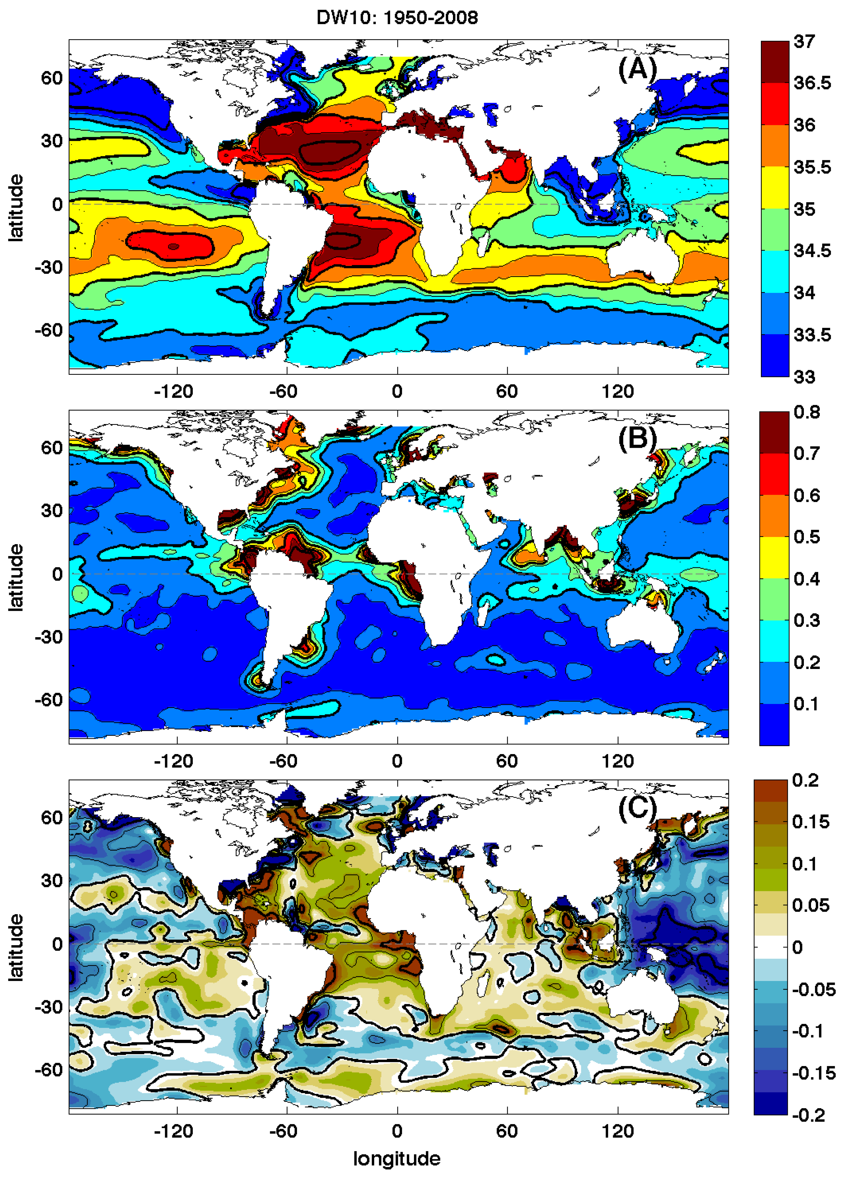
Figure 3.
Mean surface salinity for the three regimes estimated by the EM procedure using EN4 1950–2014 data: (A) Regime A: 1950–1990; (B) Regime B: 1990–2009; and (C) Regime C: 2009–2014. The right panels include the differences between the means of (D) Regime B and A; and (E) Regime C and B.
Figure 3.
Mean surface salinity for the three regimes estimated by the EM procedure using EN4 1950–2014 data: (A) Regime A: 1950–1990; (B) Regime B: 1990–2009; and (C) Regime C: 2009–2014. The right panels include the differences between the means of (D) Regime B and A; and (E) Regime C and B.

Figure 4.
Surface salinity trend (year) for the three regimes estimated by the EM procedure using EN4 1950–2014 data: (A) Regime A: 1950–1990; (B) Regime B: 1990–2009; and (C) Regime C: 2009–2014. The right panels include the differences between the trends of (D) Regimes B and A and (E) Regimes C and B. Note the different (four-times larger) color scale for (C,E).

Figure 5.
Average surface salinity time series (blue) for four example regions: (A) Equatorial Atlantic (5° S–5° N); (B) North Atlantic Subtropical Gyre (15° N–30° N); (C) Mediterranean; and (D) Equatorial Pacific (5° S–5° N). The green dashed lines indicate the separation (breakpoint) between regimes. The red lines are the average salinity for each regime, and the black lines represent the trends for each regime. The gray lines for the period 2010–2014 correspond with the SMOS data average for each region (not the Mediterranean). Note the change in the salinity range (vertical scale) in each panel.

Figure 6.
Main modes of variability of the EN4 1950–2014 salinity. First (A) and second (D) modes for Regime A (1950–1990). First (B) and second (E) modes for Regime B (1990–2009). First (C) and second (F) modes for Regime C (2009–2014). EOF, empirical orthogonal function.
Figure 6.
Main modes of variability of the EN4 1950–2014 salinity. First (A) and second (D) modes for Regime A (1950–1990). First (B) and second (E) modes for Regime B (1990–2009). First (C) and second (F) modes for Regime C (2009–2014). EOF, empirical orthogonal function.

Figure 7.
Time series of modes of variability of the EN4 1950–2014 salinity. First (A) and second (B) modes for Regime A (1950–1990), B (1990–2009) and C (2009–2014). The green dashed lines indicate the separation (breakpoint) between regimes.
Figure 7.
Time series of modes of variability of the EN4 1950–2014 salinity. First (A) and second (B) modes for Regime A (1950–1990), B (1990–2009) and C (2009–2014). The green dashed lines indicate the separation (breakpoint) between regimes.

Figure 8.
Mean surface salinity for the three regimes estimated by the EM procedure using combined EN4 and SMOS data: (A) Regime A’: 1950–1988; (B) Regime B’: 1988–2010; and (C) Regime C’: 2010–2014. The differences between the means of Regime B’ and A’ (D) and Regime C’ and B’ (E) are also included.

Figure 9.
Surface salinity trend for the three regimes estimated by the EM procedure using combined EN4 and SMOS data: (A) Regime A’: 1950–1988; (B) Regime B’: 1988–2010; and (C) Regime C’: 2010–2014. The differences between the trends of Regime B’ and A’ (D) and Regime C’ and B’ (E) are also included. Note the different (four times larger) color scale for panels (C,E).

© 2017 by the authors. Licensee MDPI, Basel, Switzerland. This article is an open access article distributed under the terms and conditions of the Creative Commons Attribution (CC BY) license (http://creativecommons.org/licenses/by/4.0/).
Share and Cite
MDPI and ACS Style
Aretxabaleta, A.L.; Smith, K.W.; Kalra, T.S. Regime Changes in Global Sea Surface Salinity Trend. J. Mar. Sci. Eng. 2017, 5, 57. https://doi.org/10.3390/jmse5040057
AMA Style
Aretxabaleta AL, Smith KW, Kalra TS. Regime Changes in Global Sea Surface Salinity Trend. Journal of Marine Science and Engineering. 2017; 5(4):57. https://doi.org/10.3390/jmse5040057
Chicago/Turabian StyleAretxabaleta, Alfredo L., Keston W. Smith, and Tarandeep S. Kalra. 2017. "Regime Changes in Global Sea Surface Salinity Trend" Journal of Marine Science and Engineering 5, no. 4: 57. https://doi.org/10.3390/jmse5040057
Note that from the first issue of 2016, this journal uses article numbers instead of page numbers. See further details here.