Spatial and Temporal Clustering Analysis of Extreme Wave Events around the UK Coastline

1
Ocean and Earth Science, National Oceanography Centre, University of Southampton, European Way, Southampton SO14 3ZH, UK
2
Department of Civil, Environmental, and Construction Engineering and Sustainable Coastal Systems Cluster, University of Central Florida, 12800 Pegasus Drive, Suite 211, Orlando, FL 32816-2450, USA
*
Author to whom correspondence should be addressed.
J. Mar. Sci. Eng. 2017, 5(3), 28; https://doi.org/10.3390/jmse5030028
Submission received: 8 May 2017
/
Revised: 26 June 2017
/
Accepted: 10 July 2017
/
Published: 14 July 2017
(This article belongs to the Special Issue Coastal Sea Levels, Impacts and Adaptation)
Abstract
:Densely populated coastal regions are vulnerable to extreme wave events, which can cause loss of life and considerable damage to coastal infrastructure and ecological assets. Here, an event-based analysis approach, across multiple sites, has been used to assess the spatial footprint and temporal clustering of extreme storm-wave events around the coast of the United Kingdom (UK). The correlated spatial and temporal characteristics of wave events are often ignored even though they amplify flood consequences. Waves that exceeded the 1 in 1-year return level were analysed from 18 different buoy records and declustered into distinct storm events. In total, 92 extreme wave events are identified for the period from 2002 (when buoys began to record) to mid-2016. The tracks of the storms of these events were also captured. Six main spatial footprints were identified in terms of extreme wave events occurrence along stretches of coastline. The majority of events were observed between November and March, with large inter-annual differences in the number of events per season associated with the West Europe Pressure Anomaly (WEPA). The 2013/14 storm season was an outlier regarding the number of wave events, their temporal clustering and return levels. The presented spatial and temporal analysis framework for extreme wave events can be applied to any coastal region with sufficient observational data and highlights the importance of developing statistical tools to accurately predict such processes.
1. Introduction
Waves are a key process influencing coastal flooding, morphology, and nearshore ecology [1]. Quantifying the variability of wave parameters is essential for coastal engineering and management [2]. Similarly, understanding wave climate and probabilities of extreme events is also crucial for offshore operators. This is emphasised, for example, by a recent increase in the planned deployment of offshore wind farms in the United Kingdom (UK) shelf seas [1]. Furthermore, the electricity generation industry is regarding wave energy as a sustainable source with considerable potential and is expanding its efforts to research wave characteristics and climate [3]. Ocean waves are also crucial for coastal flood risk management. Flooding and coastal erosion due to extreme waves and storm surges are a major hazard for coastal populations [4], as they are capable of causing extensive economic, cultural, and environmental damage, and can also be associated with high mortality [5]. A combination of high water levels (caused by spring tides and storm surges) together with waves is the primary factor leading to coastal flooding. Those combined processes can cause loss of life, and damage to property and the environment by overtopping coastal defenses and inundating low-lying areas [6]. The amount of damage rendered by coastal flooding also depends on the presence of population and infrastructure along the coast [7]. Furthermore, flood risk variability along the coast depends on the spatial characteristics of the governing processes. Many studies have demonstrated that return periods of storm tides can vary considerably along the affected coasts, e.g., [8,9,10,11], and this also applies to other nearshore processes such as waves. Hence, spatial characterization of wave processes becomes essential to manage coastal hazards effectively.
In northern Europe and the UK in particular, a remarkable series of storms occurred over the winter of 2013/14, with large waves and high sea level events affecting large stretches of the UK coast. The most significant features of this storm season were the length of coastline affected by flooding (i.e., ‘spatial footprints’) [12] and the short inter-arrival times between extreme events (i.e., ‘temporal clustering’) [13]. These issues have important implications in terms of flood risk management. Economical, societal, and environmental impacts derived from extreme events are often correlated with their spatial extent [14,15]. For instance, the action of extreme waves against ports located in nearby locations can hinder trading activities between different countries [16]. On the other hand, temporal clustering of extreme wave events may have important consequences for coastal structures due to attritional effects and insufficient time to properly repair structures between storms [17]. Similarly, natural systems such as beaches may not have enough time to recover if they are affected by many consecutive extreme events [17,18], minimizing the protection of coastal areas against flooding and leading to a wide range of economic and societal consequences [19]. These two processes are particularly relevant to the UK due to its long and irregular coastline (>1800 km) and its relatively high risk of coastal flooding: about 2.5 million people and vast economic coastal assets are considered to be exposed to coastal flooding [20]. Some studies have been undertaken to understand the extreme spatial behavior and temporal clustering of storm surges and extreme sea levels around the country, e.g., [13,15,21]. However, little attention has been paid to storm waves, which also had a large contribution to the devastating consequences observed during the winter of 2013/14. Haigh et al. [15] recently developed an ‘Event based’ analysis approach to assess the spatial footprints and temporal clustering of extreme sea levels and storm surge events around the UK. Here we build on their approach and extend it to waves.
The main aim of this paper is to assess and better understand the spatial footprints and the temporal clustering of extreme wave events to facilitate the inclusion of such information into statistical models and coastal management. We address the following four objectives: (1) compare the dates and return periods of the extreme wave events recorded around the UK; (2) assess the spatial characteristics of the wave events around the coast, distinguishing different types of footprints of events and examining the categories and tracks of the weather systems responsible for their generation; (3) investigate the temporal variation in events over different time-scales and in particular the clustering nature of extreme storm-wave events; and (4) examine these characteristics for the exceptional 2013/14 storm season.
2. Data
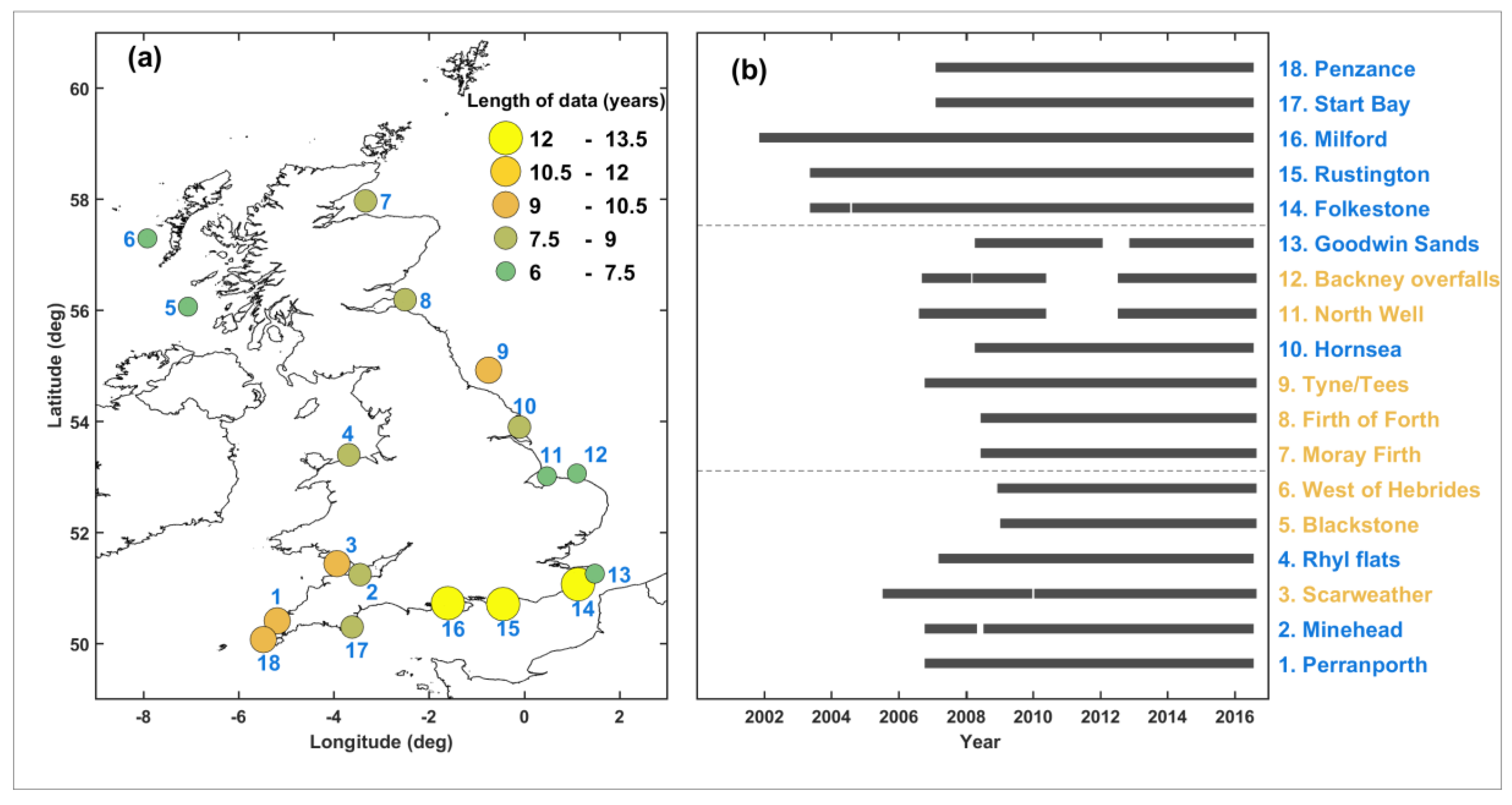
The primary dataset we use comprises wave data from Datawell’s Directional Waverider buoys. Surface-following moored wave buoys are the most abundant around the UK coastline and for consistency we only use data from this buoy type. Wave data is extracted from two different sources. We first use data from the Centre for Environment, Fisheries and Aquaculture Science (CEFAS) WaveNet Array [22], funded by the Environment agency [22,23]. The second main source is the Channel Coastal Observatory (CCO) wave array, which is composed of several wave boys located around the English Channel [24]. Wave buoys from both sources provide half-hourly data. In total, we used data from 18 buoys. The buoy data adopted in this study has been selected to comprise the buoys with the longest records and fewest gaps, whilst ensuring that the UK coastline is adequately covered (Figure 1a). The data from both sources undergo rigorous quality controls by the data operators (refer to the data sources for more information [22,24]). Values which the CCO had flagged suspicious were removed and our own extensive checks were applied to all datasets, removing spurious values. The mean data length for all considered records is nine years (Figure 1b, Table 1).
The second dataset we use is gridded mean sea level pressure and near-surface wind fields to digitise storm tracks. This global meteorological dataset is taken from the 20th Century Reanalysis, Version 2 [25], which has a spatial resolution of 2° and temporal resolution of six hours from 1871–2014 (at the time of analysis). Data for 2015 and 2016 were derived from the US National Center for Environmental Predictions/National Center for Atmospheric Research’s (NCEP/NCAR) comparable Reanalysis, Version 2 [26]. These fields have a horizontal resolution of 2.5° and were interpolated to 2° for consistency.
We use a third dataset comprising different atmospheric oscillation indices known to exert influence over the North Atlantic wave climate to assess their possible correlation with extreme storm-wave event occurrences [27]. This dataset contains: (1) the winter-averaged (December to March; DJFM) North Atlantic Oscillation (NAO) index described by Jones et al. [28] and obtained from [29]; (2) the DJFM East Atlantic Pattern (EA) index [30]; (3) the DJFM Scandinavian Pattern (SCAND) index [30]; and (4) the West Europe Pressure Anomaly (WEPA) as described by Castelle et al. [27].
3. Methodology
We followed the methodological approach developed by Haigh et al. [15], but adapted it for waves. The first stage of the analysis consisted of extracting significant wave heights that exceeded the 1 in 1-year return levels at all 18 wave buoy sites. This limit was chosen as a trade-off between identifying a large enough sample of events and still analyzing only waves that are considered ‘extreme’. We applied a range of different extreme value analysis techniques to estimate wave return levels at each site. Given the relatively short length of records (the longest one has been recording for 13 years; Figure 1b and Table 1), we found that the Peak Over Threshold (POT) method was the most appropriate to estimate return levels. Hence, we calculated the 99.75th percentile threshold based on all observations and fitted a Generalized Pareto Distribution (GPD) to the threshold exceedances. To ensure independency, we applied a declustering algorithm. Following the meteorological independence criterion [31], we applied a 3-day storm window to separate events. Comparing the GPD fits at all sites with Gringorten’s plotting positions revealed satisfactory results, i.e., the GPD performs well in modelling extreme waves (Figure 2). The significant wave heights associated with ten return periods at the 18 study sites are listed in Table 2. We then extracted all wave events, across each of the 18 sites that exceeded the 1 in 1-year return level threshold. For each wave event that reached or exceeded the threshold, we recorded the: (1) date-time of the wave event; (2) return period; (3) significant wave height; and (4) the site number.
The second stage of the analysis was to identify the distinct, extra-tropical storms that produced the extreme waves that were identified in stage one, and then to capture the meteorological information about those storms. Following the approach of Haigh et al. [15], this involved a two-step procedure. First, we used a simple ‘storm window’ approach, based on the fact that most storms that caused high waves in the UK typically lasted up to about three days. We started with the wave height associated to the highest return period, and found all of the other high waves that occurred within a window of one and a half days before or after at the other sites. We then assigned to these the event number 1. We set all high waves associated with event 1 aside and moved on to the event with the next highest return period, and so on. Second, we manually used the meteorological data to determine if our above-described procedure had correctly linked high waves to distinct storms. To achieve this, an interactive interface in MATLAB was used. This interface displayed the six-hourly progression of mean sea level pressure and wind vectors over the North Atlantic Ocean and Northern Europe around the time of maximum return period for each of the previously identified extreme events that exceeded a 1 in 1-year threshold. On all occasions, our simple procedure correctly identified distinct storms and associated wave events across the study sites. Using the same interactive MATLAB interface, the storm tracks associated with the extreme wave events were digitised, from when the low-pressure systems developed until they dissipated or moved beyond latitude 20° E. Storm tracks were captured by selecting the grid point of the lowest atmospheric pressure at each 6-h time step. From the start to the end of the storm the following 6-hourly information was stored: (1) time; (2) latitude and (3) longitude of the minimum pressure cell; and (4) the minimum mean sea level pressure.
The third stage of the methodology involved examining the results obtained in the previous stages to assess the spatial and temporal clustering features of events. For each storm event, we examined the spatial extent of extreme high waves by comparing the sites in which the 1 in 1-year return level was exceeded during the defined storm window (i.e., three days). Then, the spatial extent was compared for all events to find regional patterns regarding extreme wave occurrences and define distinct regions. We also assessed the wave spectral characteristics (provided by CCO and CEFAS) for the most significant events to determine whether events had sea, swell, or bi-modal characteristics. The temporal analysis of extreme wave events consisted of two steps. First, temporal trends of events were analysed by looking at both monthly and inter-annual changes. We compared the inter-annual changes of events with different atmospheric oscillations (NAO, EA, SCAND and WEPA), as done in previous wave climate studies on the west coast of Europe, e.g., [27,32,33,34]. Second, the temporal clustering was evaluated by comparing the time between consecutive events. The 2013/14 storm season was assessed in detail by evaluating how unusual it was in the historic (as far as data availability allows) context. The number of extreme events exceeding the 1 in 1-year return level, their actual return periods, spatial extent, and inter-arrival times were compared. A site-by-site comparison was performed for the same season to identify areas that were most affected. For correlation analyses, we use the Kendall rank correlation coefficient throughout the paper to account for integer variables.
4. Results
4.1. Wave and Storm Event Identification
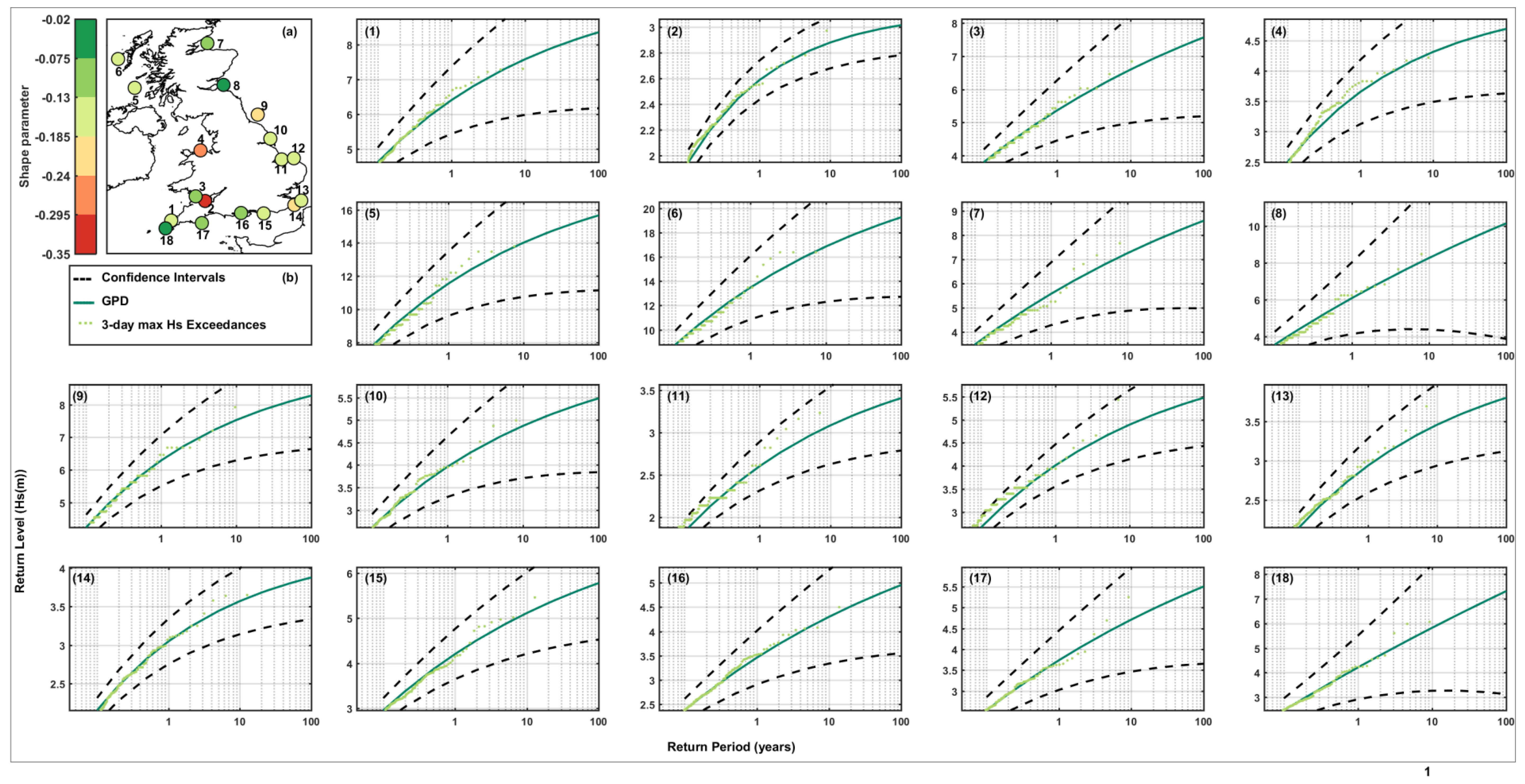
First, we compare the dates and return periods of extreme waves. In total, 165 significant wave heights were found that exceeded the 1 in 1-year return level across the 18 sites. These high wave occurrences were generated by 92 distinct storms. Comparing all storm events in terms of their highest return period across all sites, we found that 43 of the distinct 92 storm events led to wave heights around the UK with maximum return periods ranging from 1 to 2 years, 22 from 2 to 5 years, and 27 had a return period that exceeded 5 years (Figure 3). Analyzing the GPD shape parameters we find pronounced spatial variability across the 18 study sites (Figure 2a). The shape parameter is also correlated with the level of the exposure. The curve of the GPD is more pronounced at sheltered sites and vice versa, with exception of the study sites located in the northwest (NW) region. These wave buoys are located further away from the coast than others with similar level of exposure. This may lead to different behavior of the GPD shape and scale parameters. Galanis et al. [35] found that the GPD was close to a straight line (in the Gumbel space) when offshore wave data was analysed.
4.2. Spatial Footprint and Storm Track Analysis
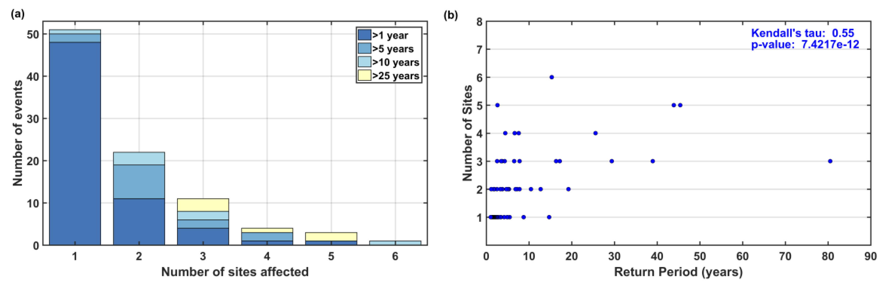
Second, we examine the spatial characteristics of waves for the 92 storm events. Initially, the number of sites where the 1 in 1-year return period was reached or exceeded during an event was analysed as well as their maximum return level. More than half of the storm-wave events (51 out of 92) led to significant wave heights with a return period greater than 1 year at only one site, of which 94% (48 out of 51) had a return period between 1 and 5 years, two events had a maximum return period between 5 and 10 years, and just one had a return period between 10 and 25 years (Figure 4a). Generally, the number of sites affected by a specific event is proportional to the maximum return period. The correlation coefficient for that relationship is 0.54 and is statistically significant at the 95% confidence level (Figure 4b).
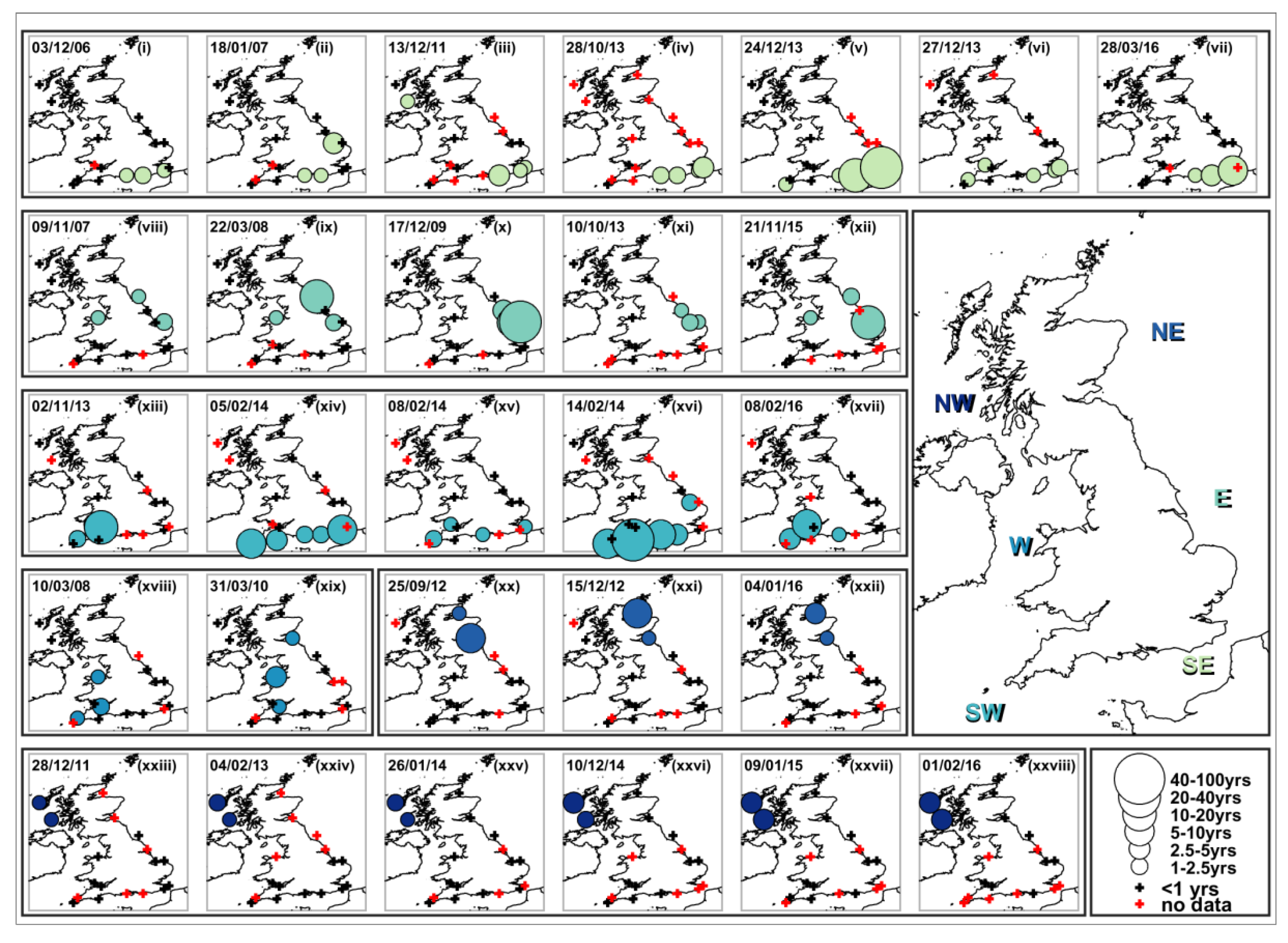
To examine the spatial patterns of extreme events along the coast we identified the most significant events, selecting those that affected several study sites (three or more sites for southern and midland study sites; two or more for northern sites due to poorer spatial resolution). Overall, our results suggest there are six categories of spatial footprints, with some overlap (Figure 5). The first type of footprint covers the southwest (SW) coast, approximately from Start Bay to Minehead (Figure 5, events xiii–xvii). The second type of footprint covers the west (W) coast, including Scarweather and Rhyl Flats in the Irish Sea (Figure 5, events xviii–xix). The third type of footprint is located in the NW of the UK (Figure 5, events xxiii–xxviii), whereas the fourth one is located in the northeast (NE) of the country (Figure 5, events xx–xxii). The fifth footprint covers the east (E) coast (Figure 5, events viii–xii), mainly including sites between Newcastle and Folkestone. The sixth footprint is located along the southeast (SE) of England, approximately between Folkestone and Milford (Figure 5, events i–vii).
We also assessed the storm tracks that led to the extreme events considered here. This was done to identify different storm types which typically affect certain coastline stretches. As outlined below, this analysis step provides valuable insights but we also note to be careful in generalizing the results because of the limited number of events that we assessed. For the SW region, storm centers at time of the highest significant wave heights were mostly located around the north of the UK, and the storms followed similar tracks (Figure 6a). We generally observe that extreme swell events are created by storm tracks coming from the SW and heading toward Scandinavia, passing through the UK diagonally. For the W region (Figure 6b), the fact that the highest return periods of both events occurred when they were located at a very similar position suggests that wind patterns have an important role in creating extreme events. Moreover, the site protected by Ireland (Rhyl Flats, Site 4) is characterized by a spectrum (not shown) which always behaved in the same manner during the considered extreme conditions, showing that extreme wave events are usually the result of winds in the Irish Sea. Storm tracks for the NW region present very similar behavior (Figure 6c), passing between Iceland and the UK with storm centers located to the NW of the UK when the highest wave heights were observed.
Storm tracks leading to extreme events in the NE region show different patterns (Figure 6d), and so does the spectral density for different periods during distinct events. It is also noteworthy that extreme events in that particular area lasted twice as long as for any other region, though the short wave time-series does not allow us to examine this characteristic properly. Regarding the E region, the most significant events had swell characteristics, and all of them occurred when the storm center was over the N of Germany, the Benelux, the N of France, or Scandinavia (Figure 6e). In the SE region, storm centers at the time of the highest waves are spread out, although they are often in the N of the UK, Ireland, or Atlantic Ocean (Figure 6f). All the considered extreme events in the SE had pronounced swell characteristics and occurred with a positive NAO phase. Similar to those in the SW region, the storm tracks usually follow the same pattern in the SE, coming from the middle of the North Atlantic and bending towards the north while passing through the UK. The most exceptional extreme events occurred when the storm track had a steady longitudinal direction, constantly heading towards the SW of the country.
4.3. Seasonality and Temporal Clustering Analysis
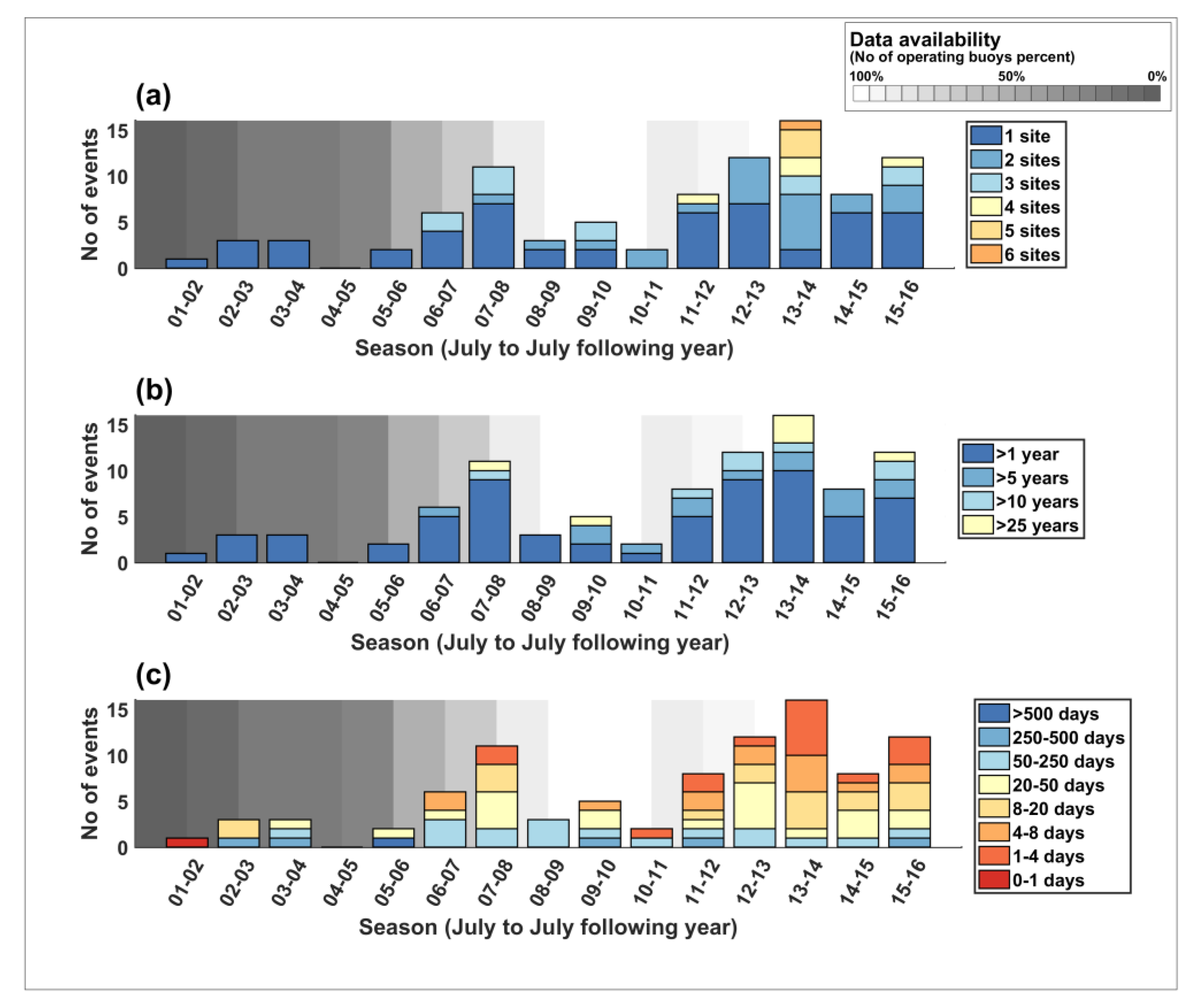
Third, we assess temporal trends and clustering of events. The number of events per season (15 July to 14 July in the following year) and the inter-seasonal changes in the number of extreme events are assessed by examining the number of sites that they affected (Figure 7a), the maximum return period that was reached (Figure 7b), and the number of days between consecutive events (Figure 7c). The 2013/14 season had the largest number of extreme events, since 2002, and was the most unusual in terms of the extent of the spatial footprints of these events, their return periods and their short inter-arrival times (see Section 4.4 for details). The seasons of 2012/13 and 2015/16 were equally important in terms of the number of extreme events that exceeded the 1 in 1-year return period, although they present different characteristics: 2012/13 extreme events affected no more than two sites at the same time and they generally had a lower return period; 2015/16 events were more severe, with one of them affecting four sites, another event with a return period that exceeded 25 years and many events with a small number of days between them. The 2007/08 season also had a relatively large number of extreme events, but was overall calmer than the seasons discussed above. The rest of the considered seasons were relatively calm, but results have to be treated with caution before 2007, owing to poor data resolution.
The number of events per month over the entire time series was examined, paying attention to the spatial footprints of the events, their maximum return period and the days between events. No events were observed in July and the number grows steadily afterwards with its maximum in December/January (Figure 8). There is a sharp drop in number of events in April, and it is notable that only a small number of events occurred in September and these were even lower than those in August. Approximately 90% of all the events happened between October and March. Also, all the events with a spatial footprint extending three or more study sites occurred in those months, as well as most of the events with a return period longer than ten years and those with inter-arrival times less than eight days. November and December are the most severe months as they had more events that exceeded the 25-year return period than any other month. These two months also feature events with the shortest time between them in the entire time series. However, February is also an exceptional month, as more than half of the events affected two sites or more.
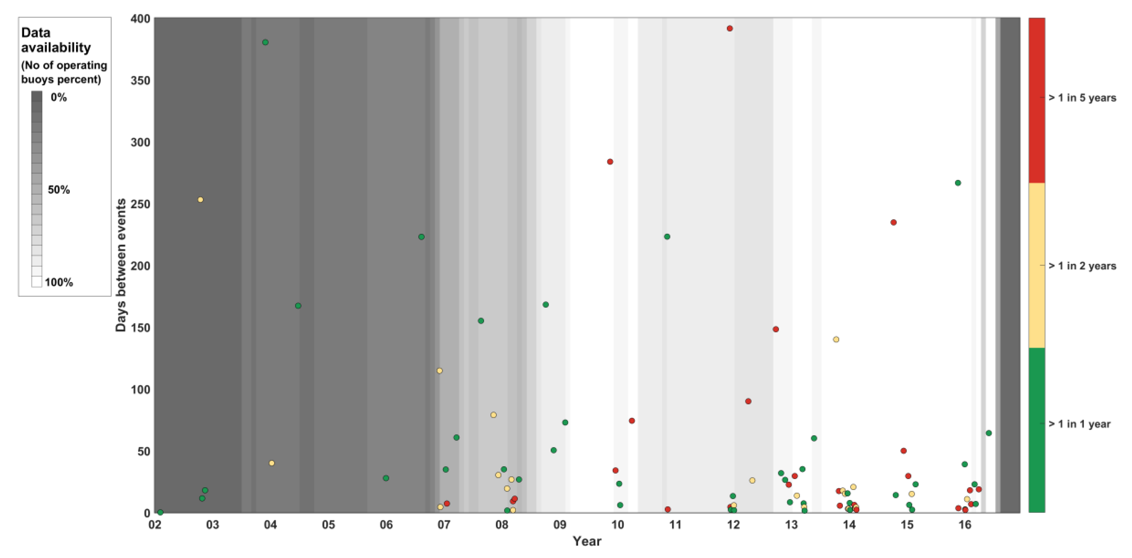
Finally, the clustering nature of storm-wave events was further evaluated comparing the days between events for the available records. This part of the analysis shows that about 15 events (16%) out of 92 occurred less than four days after the previous one, 29 (32%) less than eight days and 46 (50%) less than 20 days. As expected, events with the largest number of days between them occurred during periods of poor data resolution (Figure 9), and at the beginning of each season due to the low number of events during summer. The days between events have also been analysed for each site individually (not shown). Overall, there is a clear similarity between sites belonging to the same region. Furthermore, the correlation between the number of events per season and four atmospheric oscillation indices that affect the North Atlantic wave climate have been examined (Table 3); for that we use the rank correlation coefficient Kendall’s tau. The highest correlation exists between the WEPA index and the total number of events with a value of 0.7 (significant at 95% confidence). No significant relationship was found for the rest of the considered atmospheric indices, but the results vary spatially. The NAO index largely explains extreme wave variability in the NW of the UK and has also strong correlation with the sites located in the SE region. The EA index is strongly correlated with events observed at the eastern wave buoy sites and one site located in the SE region. The SCAND index shows high correlation at two unconnected sites, but overall this index has the smallest influence on UK extreme wave events. Finally, strong relationships are found between the WEPA index and sites that are mainly located in the E and SW regions.
4.4. The Unusual 2013/14 Season
Our last objective was to assess how unusual the 2013/14 season was for waves in the longer-term (back to 2002) context. The 2013/14 season was the most extreme, since 2002, in terms of both the total number of threshold exceedances (49) and the number of storm events that were responsible for the extreme waves (16). Although this season was the one with the highest number of extreme events, there were some other notable seasons such as the 2012/13 and 2015/16 seasons. However, the 2013/14 season generated the maximum-record significant wave heights and return periods at six sites (2, 13, 15, 16, 17, and 18), particularly in the SE and SW (Table 4). In addition, 5 out of those 6 maximum return periods are ranked in the top ten and it is the only season featuring three events with a return period higher than 25 years. The largest return period was found at site 17 (Penzance), being ranked 2nd with a return period of 45 years. This event occurred on the 14th of February 2014 and the driving storm also led to the highest return period on record in site 16 and had a large spatial footprint, affecting five sites in the SW and SE regions. Waves were reported to have reached 7.5 m at the Channel Light Vessel and caused coastal flooding along the English Channel [36].
Half of the events in the 2013/14 season affected at least three sites and only 11% of the events affected just one site. The season also featured the top four largest spatial footprints. The event with the largest footprint led to a maximum return period of 15 years that was reached at site 18 on the 5th of February 2014 and is ranked 10th but was not the maximum return period recorded for any site. During this extreme event, very large swell waves were reported breaking against the coast of West Wales, Cornwall and also parts of Northern Ireland and Scotland due to the joint action of waves and the storm surge [36].
Temporal clustering of extreme wave events was probably the most unusual characteristic of the season. Six out of 16 events occurred within less than four days, and 10 within eight days. The events with the shortest inter-arrival times occurred on the 3rd and the 6th of January 2014 and led to a maximum return period of 1.3 and 1.8 years, respectively. These events caused high waves in nearby locations: the former affected two sites (16 and 3) in the SE and SW respectively, whereas the latter affected just one site in the south (13). The first event led to wave heights in excess of 6 m at the Aberporth Buoy and nearly the same value in the Bristol Channel Buoy. The second one caused wave heights >4 m at the WaveNet Buoy in Pool bay, with periods of about 20 s. Both events caused damages to coastal structures and flood warnings [36].
Overall, the SE and SW were the most severely affected regions by both the number of events and their clustering nature. The most affected sites were sites 3, 13, and 16, where wave heights exceeded the 1 in 1-year threshold six times. Sites 1, 14, and 15 were also strongly affected, as they recorded between four and five extreme wave heights exceedances. However, some places did not experience any 1 in 1-year return value exceedance at all, such as those located in the NE and one of the sites located in the E region (sites 7, 8, and 9, respectively).
5. Discussion
Observational data has been used to investigate the spatial footprints and temporal clustering of extreme wave events around the UK. Similar to Haigh et al. [15], who analysed extreme sea levels around the UK, we find a relationship between the return period of the wave events and the number of sites they affected. The correlation coefficient is 0.5 and this is statistically significant at 95% confidence. However, the unevenly spaced distance between study sites and the differences in data length and gaps lead to an underestimation of such correlation in the present study.
Six main spatial footprint types of extreme storm-wave events were identified and classified based on the location of sites that they encompass: SW; W; NW; NE; E; and SE. However, it must be noted that it has been difficult to distinguish between the SE and SW footprints, as some extreme events affected the entire south coast and the lack of data hinders a proper assessment of possible patterns. In contrast, Haigh et al. [15] found four main regions for extreme sea levels. Nonetheless, as spatial footprint extension depends on return period for both processes, this finding could be because they used a 1 in 5-year return period threshold. Importantly, Haigh et al. [15] also found that some unconnected coastline stretches were affected by the same storm, which has also been detected for some extreme wave events. In particular, this is observed for both the W and E regions. However, the spatial resolution of buoys recording during those events is rather poor to evaluate the spatial footprints in more detail.
Generally, storm track patterns are similar within the SE, SW, W, and NW regions. The eastern regions, however, have a more irregular pattern. The storm centers at time of the highest significant wave heights typically clustered within the western regions, whereas they were more spread out in the eastern regions, which reflects the same trend as the storm track patterns. Haigh et al. [15] found a clear pattern between the location of storm centers and the occurrence of extreme sea-levels, but this trend is not as evident for extreme wave events. The fact that storm centers during the peak of the extreme sea-levels seem more synchronised could be due to a strong relationship between their generation and the storm lowest pressure, whereas waves are more related to wind velocities which do not necessarily correspond with the storm centers [37].
Most extreme wave events occur during the autumn-winter months, which agrees with the commonly observed pattern of temporal variability in wave climate in the UK [38,39,40]. Temporal clustering is especially observed around December, January, and February when the atmospheric oscillations in the North Atlantic possess a higher control over the weather patterns in the region [27,41]. Previous studies linked this North Atlantic wave climate variability to the NAO index, e.g., [1,32]. However, strong spatial differences in the NAO influence have been identified here and in other studies, e.g., [27], suggesting that other atmospheric oscillations are also important in terms of wave formation along the UK coast. Castelle et al. [27] developed a new atmospheric pressure anomaly index that optimally explains the European west coast wave climate between the UK and Portugal. Similar to them, we also found a high correlation between the winter-averaged NAO index and extreme wave conditions in the NW region. In the same way, we found that their newly proposed WEPA index explains wave extreme events in the SW region better than the NAO. Our results suggest that such atmospheric oscillations can also be used to describe the number of extreme events in different regions; this is crucial to help stakeholders and decision makers to improve planning and manage coastal hazards more effectively. Interestingly, we found spatial correlation differences in the southern study sites: WEPA is the index that optimally explains extreme event occurrences in the SW region, while the NAO index performs better in the SE. This highlights the existence of two different regions regarding extreme wave event generation in the south of England, but longer data records are needed to explore this characteristic further. The results regarding the EA and SCAND oscillations showed poor performances and scattered spatial patterns, suggesting that these indices are less representative of extreme waves in the UK.
We also examined how the distinct atmospheric indices explain wave extreme event occurrences by considering the entire UK coastline. We found that the WEPA index explains a large part of the total number of extreme events per season in the UK with a correlation coefficient of 0.7 (significant at 95% confidence). While the WEPA index seems promising to describe wave extreme event variability along the UK coast, caution must be taken when interpreting this relationship as this index has been developed to better represent wave activity in the SW region. The SW region has a larger number of wave-buoys and longer records than other regions in this study, which can introduce bias.
Our final objective was to evaluate how unusual the 2013/2014 storm season was in terms of extreme wave heights over the instrumental record, since 2002. Masselink et al. [42] performed a similar study for the west coast of Europe by using a combination of wave buoy and wave climate reanalysis datasets. While they analysed longer time periods, our study includes a more spatially complete wave buoy dataset and is hence very useful to assess spatial and temporal clustering around the UK. Masselink et al. [42] demonstrated that the 2013/14 season was the most unusual over the last 67 years for the west coast of Europe and indicated that the region between south Ireland and NW France was the most affected. Similarly, our results show that the 2013/14 season was the most unusual in the UK and the SW region was most affected. The season was an outlier regarding all three extreme event spatial footprints, event return periods, and event inter-arrival times. The WEPA index for 2013/14 also had a high value, which indicates that the strong relationship with extreme wave events also holds for that particular season [27].
Throughout the analysis and result interpretation, the available record length of the wave data time series must be taken into account as a limiting factor and source of uncertainty. Many studies have shown the control that storms possess over wave climate, e.g., [43,44,45], stating that possible changes in storminess could increase future average significant wave heights [46,47,48]. Also, some studies have stated a strong interdecadal variability in wave climate in the North Atlantic Ocean [46,49,50]. As the mean length of our buoy records is about nine years, this variability could not have been detected, which may introduce uncertainty in the estimated significant wave height return values. Another issue is the uneven spatial distribution of buoy locations, which does not allow a proper assessment of the limits of some of the spatial footprints of extreme wave events. Moreover, there is a clear difference between the spatial resolution in the southern regions and the northern ones, which may underestimate the extent of the events in the north of the country. Furthermore, wave buoys often fail during the most extreme events. This was a significant issue during the events of the 2013/14 season (Figure 5). For our study it could potentially lead to an underestimation of the spatial footprints as there could also be exceedances in other locations where the buoys were not recording. Some extreme events may not have been detected at all, if multiple buoys failed at the same time in a specific region. This would also have an effect on our temporal clustering analysis: missed extreme events can lead to an overestimation of the inter-arrival time between events.
There are several ways in which the results could be enhanced in future studies. Coastal flooding is mainly due to the joint action of waves, tides, surges, riverine, and rain processes. Many studies highlight the importance of considering the interaction between those properties [4,6,13,15,51,52]. Hence, coupling the present spatial and temporal analysis of extreme waves with extreme surge events and tides would provide a more holistic approach to deal with flooding issues. Wave data length can be improved by making use of more sources but wave data records in the UK before the WaveNet project were sparse and inconsistent [23]. Further, hindcast wave data could be used to lengthen wave buoy data, though the accuracy of those data relies on an appropriate validation. Past research, e.g., [3,48,53], as well as our own assessment highlight the necessity of high quality and longer wave data to better understand the wave climate. Similarly, spatial consistency in the way wave data are recorded is crucial to improve our understanding of coastal flood risk and planning [47].
6. Conclusions
The overall aim of this study was to assess the spatial behaviour and temporal features of extreme storm-wave events by developing a multi-site analysis and utilising observational wave data along the UK coast. Specifically, this was done by examining the ‘spatial footprint’ and ‘temporal clustering’ of events. There is little guidance in the present literature regarding the spatial behaviour of extreme wave events and their consequences when the inter-spacing between their occurrence is shorter than usual, e.g., [15,19], especially for wave events around the UK. Yet, these processes are significant for coastal flood risk and shoreline management as they can amplify damages [18].
Six main regions were found in terms of the spatial behaviour of extreme storm-wave events. As expected, there is a strong relationship between the spatial extent of wave events and their return periods. The most significant events were swell events, except for sheltered areas such as Liverpool Bay. Some storms had a constant direction and velocity for a long period, leading to extreme swell events mainly on the SW coast of the UK possibly due to ‘trapped-fetch’ processes. The most important events often occur between November and March. There are large inter-seasonal and inter-site changes in the number of extreme events and their characteristics, which are principally linked to the WEPA index. However, spatial correlation variations exist and distinct atmospheric indices perform differently along the coast of the UK [27]. The 2013/14 season has been particularly extreme in the southern regions where six study sites experienced the highest wave heights on record. For the entire time-series, the 2013/14 season was undoubtedly the outlier, considering the size of the spatial footprints of the events, their return periods and the short inter-arrival times. The incomplete and short data coverage, however, hinders a quantification of this with high statistical certainty.
The significance of this work is the novel multi-site analysis for extreme wave events. The presented approach opens the door for similar analyses of the spatial footprints of extreme wave events and their tendency to occur in clusters and is applicable to any coastal region with sufficient observational (or high quality model) data. The importance of long-term strategic monitoring of waves is shown in this paper. Advancements in wave data consistency both temporally and spatially are essential to achieve more reliable results, especially in the light of climate change and potential increase in storminess.
Acknowledgments
This work would not have been possible without the information published by CCO, which freely provides the wave data on which this study is based. We must also express our gratitude to CEFAS and especially its WaveNet project, whose wave data have also been utilised to complement those provided by CCO. Also, thanks go to Travis Manson of CCO and David Pearce of CEFAS. Their technical support has been essential to accurately interpret the wave data which is provided by their organisations. This work contributes to the objectives of the Engineering and Physical Science Research Council Flood Memory Project (grant number EP/K013513/1). T.W. has received funding from the European Union’s Horizon 2020 research and innovation program under the Marie Sklodowska-Curie grant agreement No. 658025. The work for this paper was undertaken by the lead author as a research project at the University of Southampton, as part of the Engineering in the Coastal Environment MSc.
Author Contributions
I.D.H. conceived the study and co-wrote the paper. V.M.S. performed the analysis and wrote the paper. T.W. participated in technical discussions and co-wrote the paper.
Conflicts of Interest
The authors declare no conflict of interest.
References
- Wolf, J.; Brown, J.; Howarth, M. The wave climate of Liverpool Bay—Observations and modelling. Ocean Dyn. 2011, 61, 639–655. [Google Scholar] [CrossRef]
- Tucker, M.J.; Pitt, E.G. Waves in Ocean Engineering; Elsevier: Amsterdam, The Netherlands, 2001; p. 521. [Google Scholar]
- Clément, A.; McCullen, P.; Falcão, A.; Fiorentino, A.; Gardner, F.; Hammarlund, K.; Lemonis, G.; Lewis, T.; Nielsen, K.; Petroncini, S.; et al. Wave energy in Europe: Current status and perspectives. Renew. Sustain. Energy Rev. 2002, 6, 405–431. [Google Scholar] [CrossRef]
- Wolf, J. Coupled wave and surge modelling and implications for coastal flooding. Adv. Geosci. 2008, 17, 19–22. [Google Scholar] [CrossRef]
- Jonkman, S.N.; Vrijling, J.K. Loss of life due to floods. J. Flood Risk Manag. 2008, 1, 43–56. [Google Scholar] [CrossRef]
- Wolf, J. Coastal flooding: Impacts of coupled wave-surge-tide models. Nat. Hazards 2008, 49, 241–260. [Google Scholar] [CrossRef]
- Hinton, C.; Townend, I.H.; Nicholls, R.J. Future Flooding and Coastal Erosion Risks; Thomas Telford: London, UK, 2007; Chapter 9; p. 514. [Google Scholar]
- Battjes, J.A.; Gerritsen, H. Coastal modelling for flood defence. Philos. Trans. R. Soc. Lond. A Math. Phys. Eng. Sci. 2002, 360, 1461–1475. [Google Scholar] [CrossRef] [PubMed]
- McInnes, K.L.; Hubbert, G.D.; Abbs, D.J.; Oliver, S.E. A numerical modelling study of coastal flooding. Meteorol. Atmos. Phys. 2002, 80, 217–233. [Google Scholar] [CrossRef]
- Lewis, M.; Horsburgh, K.; Bates, P.; Smith, R. Quantifying the uncertainty in future coastal flood risk estimates for the UK. J. Coast. Res. 2011, 27, 870–881. [Google Scholar] [CrossRef]
- Lewis, M.; Schumann, G.; Bates, P.; Horsburgh, K. Understanding the variability of an extreme storm tide along a coastline. Estuar. Coast. Shelf Sci. 2013, 123, 19–25. [Google Scholar] [CrossRef]
- Thorne, C. Geographies of UK flooding in 2013/4. Geogr. J. 2014, 180, 297–309. [Google Scholar] [CrossRef]
- Wadey, M.; Haigh, I.; Brown, J. A century of sea level data and the UK’s 2013/14 storm surges: An assessment of extremes and clustering using the Newlyn tide gauge record. Ocean Sci. Discuss. 2014, 11, 1995–2028. [Google Scholar] [CrossRef]
- Chailan, R.; Toulemonde, G.; Bouchette, F.; Laurent, A.; Sevault, F.; Michaud, H. Spatial Assessment of Extreme Significant Wave Heights in the Gulf of Lions. Int. Conf. Coast. Eng. 2014, 1, 17. [Google Scholar] [CrossRef]
- Haigh, I.D.; Wadey, M.P.; Wahl, T.; Ozsoy, O.; Nicholls, R.J.; Brown, J.M.; Horsburgh, K.; Goulby, B. Spatial Footprint and Temporal Clustering of Extreme Sea Level and Storm Surge Evens around the Coastline of the UK. Sci. Data 2016, 3, 160107. [Google Scholar] [CrossRef] [PubMed]
- Hall, J.W.; Tran, M.; Hickford, A.J.; Nicholls, R.J. (Eds.) The Future of National Infrastructure: A System-of-Systems Approach; Cambridge University Press: Cambridge, UK, 2016. [Google Scholar]
- Karunarathna, H.; Pender, D.; Ranasinghe, R.; Short, A.D.; Reeve, E. The effects of storm clustering on beach profile variability. Mar. Geol. 2014, 348, 103–112. [Google Scholar] [CrossRef]
- Ferreira, O. Storm groups versus extreme single storms: Predicted erosion and management consequences. J. Coast. Res. 2005, 42, 221–227. [Google Scholar]
- Mailier, P. Serial Clustering of Extratropical Cyclones. Ph.D. Thesis, Department of Meteorology, University of Reading, Reading, UK, June 2007. [Google Scholar]
- De la Vega-Leinert, A.; Nicholls, R. Potential Implications of Sea-Level Rise for Great Britain. J. Coast. Res. 2008, 242, 342–357. [Google Scholar] [CrossRef]
- Wadey, M.P.; Haigh, I.D.; Brown, J. A temporal and spatial assessment of extreme sea level events for the UK coast. In Proceedings of the International Short Conference on Advances in Extreme Value Analysis and Application to Natural Hazards (EVAN2013), Siegen, Germany, 18–20 September 2013. [Google Scholar]
- Cefas—WaveNet. Available online: http://www.cefas.co.uk/cefas-data-hub/wavenet/ (accessed on 14 July 2016).
- Hawkes, P.J.; Atkins, R.; Brampton, A.H.; Fortune, D.; Garbett, R.; Gouldby, B.P. WAVENET: Nearshore Wave Recording Network for England and Wales, Feasibility Study; HR Wallingford: Wallingford, UK, 2001. [Google Scholar]
- CCO Map Viewer & Data Search. Available online: http://www.channelcoast.org/ (accessed on 14 July 2016).
- Compo, G.P.; Whitaker, J.S.; Sardeshmukh, P.D.; Matsui, N.; Allan, R.J.; Yin, X.; Gleason, B.E.; Vose, R.S.; Rutledge, G.; Bessemoulin, P.; et al. The Twentieth Century Reanalysis Project. Q. J. R. Meteorol. Soc. 2001, 137, 1–28. [Google Scholar] [CrossRef]
- Kalnay, E.; Kanamitsu, M.; Kistler, R.; Collins, W.; Deaven, D.; Gandin, L.; Iredell, M.; Saha, S.; White, G.; Woollen, J.; et al. The NCEP/NCAR 40-Year Re analysis Project. Bull. Am. Meteorol. Soc. 1996, 77, 437–471. [Google Scholar] [CrossRef]
- Castelle, B.; Dodet, G.; Masselink, G.; Scott, T. A new climate index controlling winter wave activity along the Atlantic coast of Europe: The West Europe Pressure Anomaly. Geophys. Res. Lett. 2017, 44, 1384–1392. [Google Scholar] [CrossRef]
- Jones, P.D.; Jonsson, T.; Wheeler, D. Extension to the North Atlantic Oscillation using early instrumental pressure observations from Gibraltar and South-West Iceland. Int. J. Climatol. 1997, 17, 1433–1450. [Google Scholar] [CrossRef]
- NAO Data. Available online: https://crudata.uea.ac.uk/cru/data/nao/ (accessed on 18 June 2017).
- Climate Prediction Center—Monitoring & Data Index. Available online: http://www.cpc.ncep.noaa.gov/data/ (accessed on 18 June 2017).
- Paolo, C.; Coco, G. (Eds.) Coastal Storms: Processes and Impacts; John Wiley & Sons: Hoboken, NJ, USA, 2017. [Google Scholar]
- Bacon, S.; Carter, D. A connection between mean wave height and atmospheric pressure gradient in the North Atlantic. Int. J. Climatol. 1993, 13, 423–436. [Google Scholar] [CrossRef]
- Bauer, E. Inter-annual changes of the ocean wave variability in the North Atlantic and in the North Sea. Clim. Res. 2001, 18, 63–69. [Google Scholar] [CrossRef]
- Masselink, G.; Austin, M.; Scott, T.; Poate, T.; Russell, P. Role of wave forcing, storms and NAO in outer bar dynamics on a high-energy, macro-tidal beach. Geomorphology 2014, 226, 76–93. [Google Scholar] [CrossRef]
- Galanis, G.; Chu, P.; Kallos, G.; Kuo, Y.; Dodson, C. Wave height characteristics in the north Atlantic Ocean: A new approach based on statistical and geometrical techniques. Stoch. Environ. Res. Risk Assess. 2011, 26, 83–103. [Google Scholar] [CrossRef]
- Sibley, A.; Cox, D.; Titley, H. Coastal flooding in England and Wales from Atlantic and North Sea storms during the 2013/2014 winter. Weather 2015, 70, 62–70. [Google Scholar] [CrossRef]
- Nissen, K.; Leckebusch, G.; Pinto, J.; Renggli, D.; Ulbrich, S.; Ulbrich, U. Cyclones causing wind storms in the Mediterranean: Characteristics, trends and links to large-scale patterns. Nat. Hazards Earth Syst. Sci. 2010, 10, 1379–1391. [Google Scholar] [CrossRef]
- Woolf, D.K.; Challenor, P.G.; Cotton, P.D. Variability and predictability of the North Atlantic wave climate. J. Geophys. Res. 2002, 107, 3145. [Google Scholar] [CrossRef]
- Van Nieuwkoop, J.; Smith, H.; Smith, G.; Johanning, L. Wave resource assessment along the Cornish coast (UK) from a 23-year hindcast dataset validated against buoy measurements. Renew. Energy 2013, 58, 1–14. [Google Scholar] [CrossRef]
- Venugopal, V.; Nemalidinne, R. Wave resource assessment for Scottish waters using a large scale North Atlantic spectral wave model. Renew. Energy 2015, 76, 503–525. [Google Scholar] [CrossRef]
- Wolf, J.; Woolf, D.K. Storms and Waves. MCCIP Annual Report Card 2010–11; MCCIP Science Review: Suffolk, UK, 2010; p. 15. [Google Scholar]
- Masselink, G.; Castelle, B.; Scott, T.; Dodet, G.; Suanez, S.; Jackson, D.; Floc’h, F. Extreme wave activity during 2013/2014 winter and morphological impacts along the Atlantic coast of Europe. Geophys. Res. Lett. 2016, 43, 2135–2143. [Google Scholar] [CrossRef]
- Wiegel, R.L. Oceanographical Engineering; Courier Corporation: North Chelmsford, MA, USA, 2013. [Google Scholar]
- Young, I.R. Wind Generated Ocean Waves; Elsevier: Amsterdam, The Netherlands, 1999; Volume 2. [Google Scholar]
- Dodet, G.; Bertin, X.; Taborda, R. Wave climate variability in the North-East Atlantic Ocean over the last six decades. Ocean Model. 2010, 31, 120–131. [Google Scholar] [CrossRef]
- Wolf, J.; Woolf, D. Waves and climate change in the north-east Atlantic. Geophys. Res. Lett. 2006, 33, L06604. [Google Scholar] [CrossRef]
- Lowe, J.A.; Howard, T.; Pardaens, A.; Tinker, J.; Holt, J.; Wakelin, S.; Milne, G.; Leak, J.; Wolf, J.; Horsburgh, K.; et al. UK Climate Projections Science Report: Marine and Coastal Projections; Met Office Hadley Centre: Exeter, UK, 2009. [Google Scholar]
- Mori, N.; Yasuda, T.; Mase, H.; Tom, T.; Oku, Y. Projection of Extreme Wave Climate Change under Global Warming. Hydrol. Res. Lett. 2010, 4, 15–19. [Google Scholar] [CrossRef]
- Gulev, S.; Hasse, L. Changes of wind waves in the North Atlantic over the last 30 years. Int. J. Climatol. 1999, 19, 1091–1117. [Google Scholar] [CrossRef]
- Sterl, A.; Caires, S. Climatology, variability and extrema of ocean waves: The Web-based KNMI/ERA-40 wave atlas. Int. J. Climatol. 2005, 25, 963–977. [Google Scholar] [CrossRef]
- Ozer, J.; Padilla-Hernández, R.; Monbaliu, J.; Alvarez Fanjul, E.; Carretero Albiach, J.; Osuna, P.; Yu, J.; Wolf, J. A coupling module for tides, surges and waves. Coast. Eng. 2000, 41, 95–124. [Google Scholar] [CrossRef]
- Bunya, S.; Dietrich, J.; Westerink, J.; Ebersole, B.; Smith, J.; Atkinson, J.; Jensen, R.; Resio, D.; Luettich, R.; Dawson, C.; et al. A High-Resolution Coupled Riverine Flow, Tide, Wind, Wind Wave, and Storm Surge Model for Southern Louisiana and Mississippi. Part I: Model Development and Validation. Mon. Weather Rev. 2010, 138, 345–377. [Google Scholar] [CrossRef]
- Jane, R.; Dalla Valle, L.; Simmonds, D.; Raby, A. A copula-based approach for the estimation of wave height records through spatial correlation. Coast. Eng. 2016, 117, 1–18. [Google Scholar] [CrossRef]
Figure 1.
(a) Location of the selected buoys and their assigned number. (b) Location names and duration of the buoy records. Yellow: Centre for Environment, Fisheries and Aquaculture Science (CEFAS) WaveNet network; Blue: Channel Coastal Observatory (CCO) wave array.
Figure 1.
(a) Location of the selected buoys and their assigned number. (b) Location names and duration of the buoy records. Yellow: Centre for Environment, Fisheries and Aquaculture Science (CEFAS) WaveNet network; Blue: Channel Coastal Observatory (CCO) wave array.

Figure 2.
Generalized Pareto Distribution (GPD) fits are shown for each of the sites along with their confidence intervals (95%). The number in brackets indicates the site identity number. Both colours and dots represent the shape parameter for each location on a UK map (a), and there is a legend for the GPD plots (b).

Figure 3.
Maximum return period per event plotted against occurrence date. The grey color of the background represents the percentage of number of sites recording: the lighter the grey, the more data are available.
Figure 3.
Maximum return period per event plotted against occurrence date. The grey color of the background represents the percentage of number of sites recording: the lighter the grey, the more data are available.
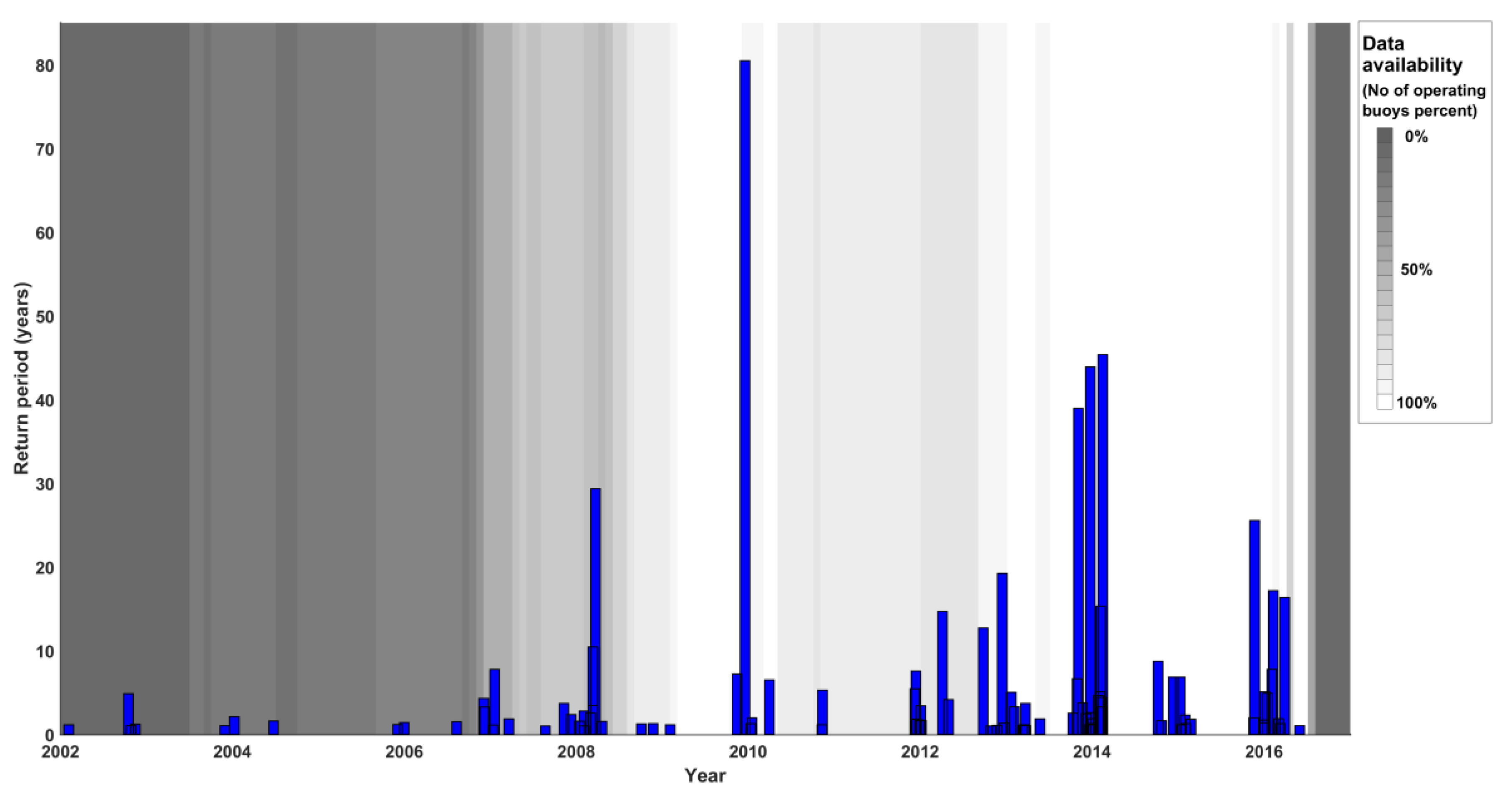
Figure 4.
(a) Histograms showing the number of sites where the 1 in 1-year return level was exceeded. Events are also sorted by different return period thresholds. (b) The return period of the highest significant wave height for the 92 extreme wave events plotted against the number of sites where the 1 in 1-year return level was exceeded.

Figure 5.
The spatial footprint of extreme events that affected three buoy sites (or two sites for the north of the UK). The events have been organized according to the regions they affected and subfigures have been sorted by date of occurrence within regions. The first number in the top left corner indicates the date on which they occurred and the Roman number in brackets is a label for each subfigure.

Figure 6.
Storm tracks that generated the extreme wave events shown in Figure 5 for the distinct six regions identified: (a) SW region; (b) W region; (c) NW region; (d) NE region; (e) E region; and (f) SE region. The grey dots indicate where the storm centers were when the maximum significant wave height occurred.
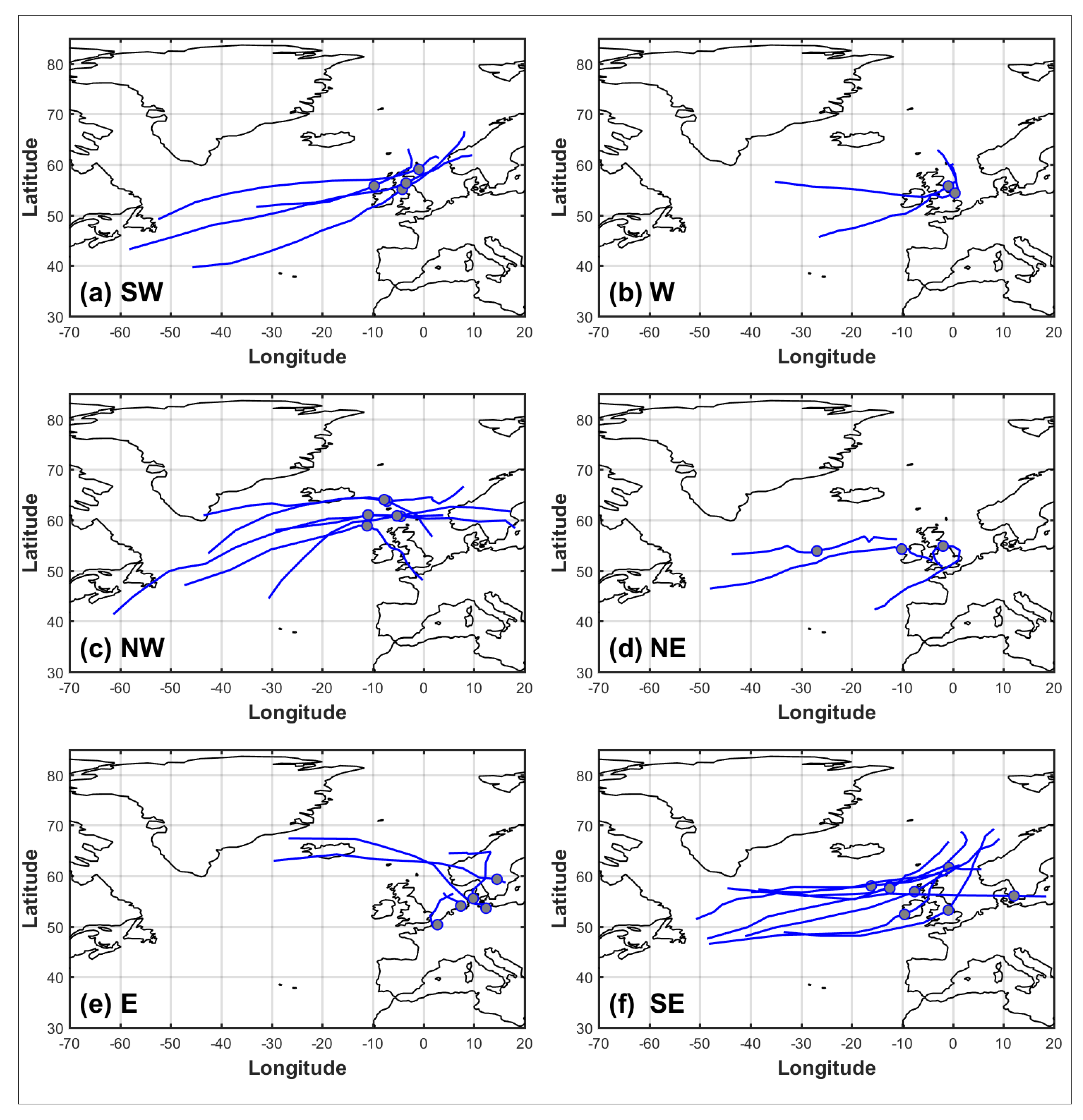
Figure 7.
Number of significant wave height extreme events per season (July to July of the next year) for (a) distinct number of sites affected (i.e., spatial footprint), (b) different return level thresholds, and (c) ranges of days between events. The grey shading at the background represents the mean annual data availability: they lighter the grey, the more data are available.

Figure 8.
Number of significant wave height extreme events per month for (a) distinct number of sites affected (i.e., spatial footprint), (b) different return level threshold, and (c) ranges of days between events.
Figure 8.
Number of significant wave height extreme events per month for (a) distinct number of sites affected (i.e., spatial footprint), (b) different return level threshold, and (c) ranges of days between events.
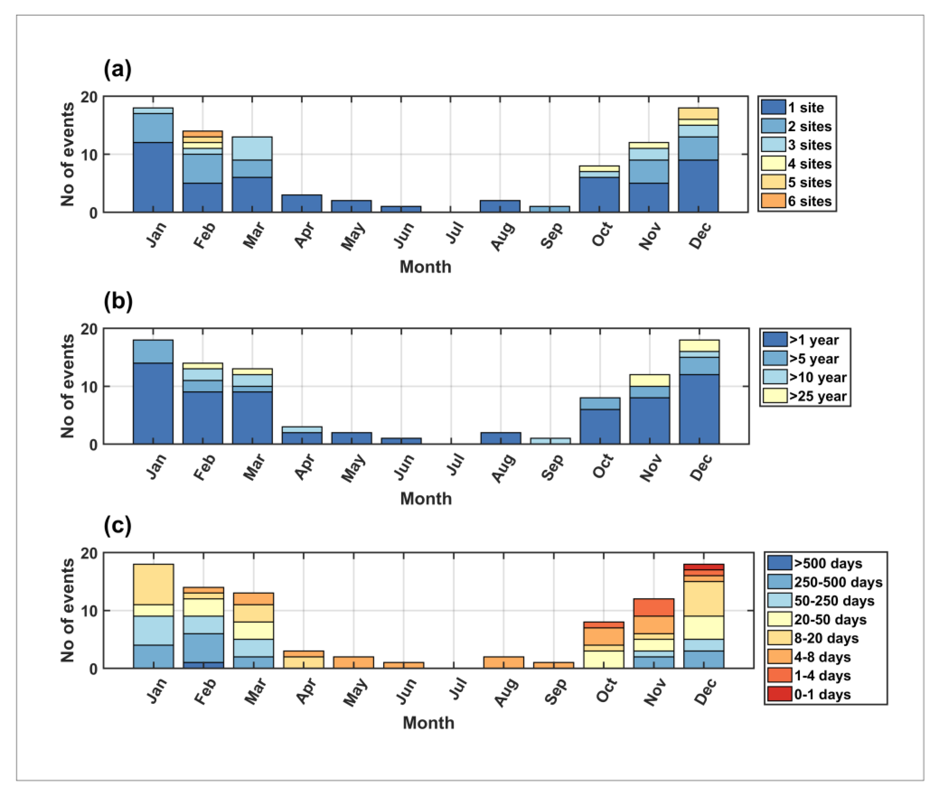
Figure 9.
Number of days between consecutive significant wave height extreme events for all sites, showing different return level thresholds for each event. The grey shading at the background of the figures represents the percentage of number of sites for which data are available: the lighter the grey, the more data are available.


Table 1.
Name, location, data length, depth, and distance from the coast for each study site.
| Site Number | Site Name | Longitude (deg.) | Latitude (deg.) | Range | Number of Years (Data Range) | Depth (m CD) | Distance to Coast (km) |
|---|---|---|---|---|---|---|---|
| 1 | Perranporth | −5.188 | 50.403 | 2006–2016 | 9.1 (10.5) | 10 | 2.1 |
| 2 | Minehead | −3.449 | 51.235 | 2006–2016 | 8.7 (10.5) | 10 | 3.1 |
| 3 | Scarweather | −3.933 | 51.433 | 2005–2016 | 10.2 (11.9) | 35 | 14.7 |
| 4 | Rhyl Flats | −3.686 | 53.393 | 2007–2016 | 8.4 (10.2) | 10 | 9.5 |
| 5 | Blackstone | −7.062 | 56.062 | 2009–2016 | 7.3 (8.4) | 97 | 43.6 |
| 6 | West of Hebrides | −7.914 | 57.292 | 2009–2016 | 7.2 (8.4) | 100 | 29.6 |
| 7 | Moray Firth | −3.333 | 57.966 | 2008–2016 | 7.7 (8.9) | 54 | 26.9 |
| 8 | Firth of Forth | −2.504 | 56.188 | 2008–2016 | 7.8 (8.9) | 65 | 2.7 |
| 9 | Tyne/Tees | −0.749 | 54.919 | 2006–2016 | 9.5 (10.6) | 65 | 39.2 |
| 10 | Hornsea | −0.102 | 53.893 | 2008–2016 | 7.8 (9.1) | 12 | 2.95 |
| 11 | NorthWell | 0.475 | 53.008 | 2006–2016 | 6.8 (10.8) | 31 | 6.3 |
| 12 | Backney Overfalls | 1.104 | 53.058 | 2006–2016 | 6.9 (10.7) | 23 | 10.9 |
| 13 | Goodwin Sands | 1.483 | 51.252 | 2008–2016 | 6.8 (9) | 10 | 4.3 |
| 14 | Folkestone | 1.128 | 51.063 | 2003–2016 | 12.3 (14) | 13 | 0.79 |
| 15 | Rustington | −0.445 | 50.704 | 2003–2016 | 12.4 (14) | 9.9 | 8.8 |
| 16 | Milford | −1.604 | 50.721 | 2002–2016 | 13.1 (15.5) | 10 | 0.5 |
| 17 | Start Bay | −3.616 | 50.292 | 2007–2016 | 9 (10.2) | 10 | 1.5 |
| 18 | Penzance | −5.478 | 50.066 | 2007–2016 | 9 (10.2) | 10 | 5.4 |
Table 2.
Hs return level estimates (meters) for each of the 18 study sites for different return periods.
Table 2.
Hs return level estimates (meters) for each of the 18 study sites for different return periods.
| Site Number | Site Name | Return Period (Years) | |||||||||
|---|---|---|---|---|---|---|---|---|---|---|---|
| 0.5 | 1 | 2 | 5 | 10 | 20 | 25 | 50 | 75 | 100 | ||
| 1 | Perranporth | 5.94 | 6.40 | 6.81 | 7.27 | 7.57 | 7.84 | 7.92 | 8.15 | 8.27 | 8.35 |
| 2 | Minehead | 2.44 | 2.59 | 2.70 | 2.81 | 2.88 | 2.93 | 2.95 | 2.98 | 3.00 | 3.01 |
| 3 | Scarweather | 4.93 | 5.37 | 5.77 | 6.25 | 6.59 | 6.91 | 7.01 | 7.30 | 7.46 | 7.57 |
| 4 | Rhyl Flats | 3.37 | 3.65 | 3.89 | 4.15 | 4.32 | 4.45 | 4.49 | 4.60 | 4.66 | 4.69 |
| 5 | Blackstone | 10.61 | 11.57 | 12.41 | 13.39 | 14.02 | 14.59 | 14.76 | 15.24 | 15.49 | 15.66 |
| 6 | West of Hebrides | 12.24 | 13.49 | 14.63 | 15.97 | 16.87 | 17.68 | 17.93 | 18.64 | 19.02 | 19.28 |
| 7 | Moray Firth | 4.99 | 5.57 | 6.12 | 6.78 | 7.25 | 7.69 | 7.82 | 8.22 | 8.44 | 8.59 |
| 8 | Firth ofForth | 5.37 | 6.09 | 6.78 | 7.65 | 8.27 | 8.87 | 9.06 | 9.62 | 9.94 | 10.16 |
| 9 | Tyne/Tees | 5.78 | 6.29 | 6.73 | 7.22 | 7.53 | 7.79 | 7.87 | 8.09 | 8.20 | 8.27 |
| 10 | Hornsea | 3.61 | 3.96 | 4.28 | 4.64 | 4.87 | 5.08 | 5.15 | 5.33 | 5.42 | 5.48 |
| 11 | NorthWell | 2.42 | 2.60 | 2.77 | 2.96 | 3.08 | 3.19 | 3.23 | 3.32 | 3.37 | 3.40 |
| 12 | Backney Overfalls | 3.67 | 4.01 | 4.32 | 4.67 | 4.89 | 5.09 | 5.15 | 5.32 | 5.41 | 5.47 |
| 13 | Goodwin Sands | 2.74 | 2.94 | 3.12 | 3.32 | 3.46 | 3.57 | 3.61 | 3.71 | 3.76 | 3.80 |
| 14 | Folkestone | 2.83 | 3.05 | 3.24 | 3.44 | 3.57 | 3.68 | 3.71 | 3.80 | 3.85 | 3.88 |
| 15 | Rustington | 3.87 | 4.20 | 4.51 | 4.87 | 5.12 | 5.34 | 5.40 | 5.60 | 5.71 | 5.78 |
| 16 | Milford | 3.16 | 3.46 | 3.73 | 4.07 | 4.30 | 4.52 | 4.58 | 4.78 | 4.88 | 4.96 |
| 17 | Start Bay | 3.40 | 3.74 | 4.05 | 4.44 | 4.71 | 4.97 | 5.05 | 5.28 | 5.42 | 5.51 |
| 18 | Penzance | 3.70 | 4.21 | 4.71 | 5.35 | 5.82 | 6.28 | 6.43 | 6.87 | 7.13 | 7.31 |
Table 3.
Kendall rank correlation coefficient between the number of extreme wave events that exceeded the 1 in 1-year return level against different atmospheric oscillations indices known to exert influence over the wave climate in the Atlantic Ocean.
Table 3.
Kendall rank correlation coefficient between the number of extreme wave events that exceeded the 1 in 1-year return level against different atmospheric oscillations indices known to exert influence over the wave climate in the Atlantic Ocean.
| Site Number | NAO | EA | SCAND | WEPA | ||||
|---|---|---|---|---|---|---|---|---|
| Kendall’s Tau | p-Value | Kendall’s Tau | p-Value | Kendall’s Tau | p-Value | Kendall’s Tau | p-Value | |
| 1 | 0.57 | 0.03 | 0.26 | 0.34 | −0.31 | 0.26 | 0.39 | 0.14 |
| 2 | 0.48 | 0.08 | 0.34 | 0.22 | −0.02 | 1.00 | 0.34 | 0.22 |
| 3 | 0.32 | 0.21 | 0.54 | 0.03 | −0.47 | 0.06 | 0.51 | 0.04 |
| 4 | 0.00 | 1.00 | 0.16 | 0.63 | −0.11 | 0.77 | 0.16 | 0.63 |
| 5 | 0.83 | 0.00 | 0.04 | 1.00 | −0.12 | 0.80 | 0.20 | 0.62 |
| 6 | 0.56 | 0.10 | 0.22 | 0.60 | −0.22 | 0.60 | 0.30 | 0.43 |
| 7 | 0.00 | 1.00 | 0.30 | 0.40 | −0.15 | 0.72 | 0.30 | 0.40 |
| 8 | −0.61 | 0.04 | 0.07 | 0.91 | 0.20 | 0.58 | 0.00 | 1.00 |
| 9 | 0.02 | 1.00 | 0.11 | 0.74 | −0.37 | 0.18 | 0.32 | 0.24 |
| 10 | −0.39 | 0.22 | −0.13 | 0.74 | 0.85 | 0.00 | −0.07 | 0.91 |
| 11 | 0.08 | 0.85 | 0.60 | 0.04 | −0.18 | 0.57 | 0.75 | 0.01 |
| 12 | 0.03 | 1.00 | 0.55 | 0.06 | −0.14 | 0.68 | 0.49 | 0.10 |
| 13 | 0.68 | 0.04 | 0.37 | 0.36 | 0.05 | 1.00 | 0.26 | 0.54 |
| 14 | 0.39 | 0.08 | 0.21 | 0.37 | −0.21 | 0.37 | 0.30 | 0.19 |
| 15 | 0.55 | 0.02 | 0.33 | 0.17 | −0.17 | 0.49 | 0.40 | 0.10 |
| 16 | 0.28 | 0.20 | 0.46 | 0.03 | 0.08 | 0.75 | 0.37 | 0.09 |
| 17 | 0.42 | 0.16 | 0.14 | 0.69 | 0.08 | 0.84 | 0.53 | 0.07 |
| 18 | −0.08 | 0.85 | 0.39 | 0.17 | 0.23 | 0.44 | 0.54 | 0.05 |
| All sites | 0.36 | 0.07 | 0.36 | 0.07 | 0.05 | 0.84 | 0.70 | 0.00 |
Table 4.
Name, location, and wave variable characteristics for each of the sites.
| Site Number | Site Name | Mean Hs (m) | H0 (m) | Mean Tz (s) | Mean Tp (s) | Max Hs (m) | Max Return Period (years) | Date of Max Return Period |
|---|---|---|---|---|---|---|---|---|
| 1 | Perranporth | 1.56 | 1.71 | 5.81 | 10.47 | 7.3 | 5.30 | 8 February 2016 06:30 |
| 2 | Minehead | 0.56 | 0.58 | 3.99 | 6.51 | 2.97 | 38.96 | 2 November 2013 20:00 |
| 3 | Scarweather | 1.24 | 1.24 | 4.85 | 8.73 | 6.84 | 17.20 | 8 February 2016 15:00 |
| 4 | Rhyl Flats | 0.69 | 0.69 | 3.21 | 4.29 | 4.22 | 6.53 | 31 March 2010 10:00 |
| 5 | Blackstone | 2.59 | 2.59 | 6.38 | 10.64 | 13.8 | 7.78 | 1 February 2016 21:30 |
| 6 | West of Hebrides | 2.94 | 2.94 | 6.73 | 11.00 | 16.39 | 6.85 | 1 February 2016 18:30 |
| 7 | Moray Firth | 1.10 | 1.10 | 4.21 | 7.21 | 7.66 | 19.24 | 15 December 2012 01:30 |
| 8 | Firth of Forth | 1.04 | 1.04 | 4.27 | 6.87 | 8.48 | 12.73 | 25 September 2012 08:00 |
| 9 | Tyne/Tees | 1.34 | 1.34 | 4.64 | 7.47 | 7.92 | 29.37 | 22 March 2008 02:30 |
| 10 | Hornsea | 0.83 | 0.84 | 4.10 | 7.24 | 4.99 | 14.72 | 4 April 2012 04:30 |
| 11 | NorthWell | 0.64 | 0.64 | 3.35 | 4.50 | 3.23 | 25.57 | 21 November 2015 08:30 |
| 12 | Backney Overfalls | 0.92 | 0.92 | 3.87 | 5.99 | 5.43 | 80.51 | 17 December 2009 20:00 |
| 13 | Goodwin Sands | 0.67 | 0.67 | 3.57 | 5.21 | 3.69 | 43.89 | 24 December 2013 02:30 |
| 14 | Folkestone | 0.58 | 0.58 | 3.55 | 5.19 | 3.65 | 16.35 | 28 March 2016 04:30 |
| 15 | Rustington | 0.82 | 0.84 | 3.77 | 6.44 | 5.46 | 30.47 | 24 December 2013 02:30 |
| 16 | Milford | 0.64 | 0.67 | 4.19 | 8.18 | 4.5 | 19.06 | 14 February 2014 22:30 |
| 17 | Start Bay | 0.70 | 0.73 | 4.39 | 8.07 | 5.25 | 45.40 | 14 February 2014 21:30 |
| 18 | Penzance | 0.64 | 0.67 | 4.43 | 8.62 | 6.06 | 14.43 | 4 February 2014 19:00 |
© 2017 by the authors. Licensee MDPI, Basel, Switzerland. This article is an open access article distributed under the terms and conditions of the Creative Commons Attribution (CC BY) license (http://creativecommons.org/licenses/by/4.0/).
Share and Cite
MDPI and ACS Style
Malagon Santos, V.; Haigh, I.D.; Wahl, T. Spatial and Temporal Clustering Analysis of Extreme Wave Events around the UK Coastline. J. Mar. Sci. Eng. 2017, 5, 28. https://doi.org/10.3390/jmse5030028
AMA Style
Malagon Santos V, Haigh ID, Wahl T. Spatial and Temporal Clustering Analysis of Extreme Wave Events around the UK Coastline. Journal of Marine Science and Engineering. 2017; 5(3):28. https://doi.org/10.3390/jmse5030028
Chicago/Turabian StyleMalagon Santos, Victor, Ivan D. Haigh, and Thomas Wahl. 2017. "Spatial and Temporal Clustering Analysis of Extreme Wave Events around the UK Coastline" Journal of Marine Science and Engineering 5, no. 3: 28. https://doi.org/10.3390/jmse5030028
Note that from the first issue of 2016, this journal uses article numbers instead of page numbers. See further details here.