Scheduling of Maintenance Tasks and Routing of a Joint Vessel Fleet for Multiple Offshore Wind Farms

Abstract

Maintenance costs related to offshore wind farms are severely limiting their potential for being profitable. This paper proposes a new mathematical model that considers how maintenance tasks should be scheduled and performed by technicians transported using a fleet of dedicated vessels. The model is novel in its combination of modelling several work shifts and including vessels that can stay offshore for several shifts, while handling large maintenance tasks and accurate calculation of downtime costs. Simulation is used to evaluate the performance of the model in its pure form, as well as when solved heuristically using a rolling horizon heuristic. The results indicate that the end-of-horizon effects of the mathematical formulation are handled effectively. Computational experiments also illustrate how the mathematical model coupled with simulation can be used to evaluate strategic decisions regarding the composition of a vessel fleet used to execute maintenance tasks.

1. Introduction

Global electricity demand is increasing rapidly [1]. Wind power is among the fastest growing electrical generation systems in the world [2] and is expected to contribute substantially to the future energy consumption [3]. Wind power generation is driven offshore by several factors. One of the most important factors is space, as space is quickly becoming scarce for the installation of onshore wind turbines. Moving offshore gives the benefit of greater areas available for the installation of wind farms, it also allows for larger wind farms and for installation close to major urban cities. Installing wind turbines far from shore reduces the noise and visual impact. This will, in combination with less space restrictions, make it possible to use other designs for the turbine to improve efficiency [4]. There are generally higher wind speeds offshore than onshore, which results in a greater energy potential for offshore turbines. An onshore turbine normally has around 2000–2300 full load hours per year while an offshore turbine normally reaches more than 3000 full load hours [5,6]. It is expected that future wind farms will be located even further offshore than wind farms operating today, and that they will increase in wind turbine capacity [7]. Between 2011 and 2014 the installed capacity of offshore wind more than doubled [8].

Offshore wind energy is still far more costly than conventional energy sources [3], approximately 50% more expensive than onshore wind energy, and is dependent on governmental subsidies [5,6]. This is to a large extent due to higher installation costs, but also due to higher operation and maintenance (O&M) costs. O&M can account for up to a third of the overall lifetime costs for an offshore wind farm [9]. O&M costs include transportation costs, technician salaries and costs of repair actions and spare parts. They also include loss of revenue caused by production stop when a turbine is shut down during failures and maintenance operations. The high O&M costs of offshore wind are caused by rougher conditions than for onshore turbines. Rougher weather and salty water make offshore wind turbines more exposed to breakdowns. Rough weather and greater distances from shore also makes the turbines more difficult and expensive to access, and performance of maintenance is dependent on periods of good weather [4]. Difficulties of accessing turbines to repair failures may lead to long periods of downtime for the turbines and this can cause large financial losses.

The costs of offshore wind must be reduced in order to achieve a competitive price in the market. As O&M costs account for a substantial part of the total costs for offshore wind, a reduction of these costs is crucial to bring down the total costs. This is even more important for future wind farms, where installation further offshore decreases turbine accessibility and increases O&M costs. Efficient use of the maintenance vessel fleet and maximum utilization of periods of good weather is important to minimize the O&M costs. This creates a demand for effective scheduling of the maintenance activities.

The contributions in this paper include: (1) presenting a novel mathematical model for the scheduling and routing of vessels to perform maintenance activities across multiple wind farms over several periods, modelling both vessels that must return to an onshore depot between each shift and vessels that can stay offshore for multiple periods without going back to the depot; (2) using simulations to evaluate the tactical planning model, where new maintenance operations appear over the simulation horizon, including actual needs for maintenance as a result of alarms; (3) analyzing a rolling horizon heuristic and the use of symmetry breaking constraints to reduce runtimes when solving the mathematical model; (4) showing that the mathematical model coupled with simulations can be used to evaluate strategic decisions regarding the size and mix of vessel fleets used to conduct maintenance.

Existing literature presents several related contributions. A review of the state-of-the-art of maintenance logistics in the offshore wind industry per 2014 is given by Shafiee in [10]. Much research has been done regarding optimal offshore wind farm design. Several papers present optimization models where maintenance and repair costs are included, such as the models by Chen and MacDonald [11] and Afanasyeva et al. [12]. There is also some literature on the selection of maintenance strategies. Maintenance strategies are studied for example by Karyotakis [13] and Besnard [14]. An example of a specific field of interest within maintenance strategies are opportunistic maintenance strategies, investigated by among others Ding and Tian [15,16]. Besnard et al. [17] present a model that determines the optimal location of maintenance accommodations in combination with other maintenance support organization aspects. Poore and Walford [18] introduced and studied maintenance outsourcing.

An overview of decision support models for O&M strategies for offshore wind farms is given by Hofmann [19]. A majority of these models use simulation tools to analyze O&M related costs, and the use of optimization models for analyzing O&M costs are limited. Halvorsen-Weare et al. [20], Gundegjerde et al. [21] and Stålhane et al. [22] use optimization models to investigate vessel fleets and determine the optimal fleet size and mix for an offshore wind farm. These models can be used as support when deciding when and how many vessels to purchase or rent, addressing decisions on a strategic level for O&M in offshore wind farms.

Dai et al. [23] present an optimization model for the routing and scheduling problem of a given vessel fleet for O&M in an offshore wind farm. The model minimizes costs related to travelling to the respective turbines and delaying tasks. The time aspect of the model is a finite, short planning horizon, discretized in shorter time steps (days or shifts). It allows for tasks being performed in parallel and includes pick-up and delivery of personnel. The model only considers vessels that must return to an onshore depot between each time period. Irawan et al. [24] presents a similar model but includes technicians and capacities at onshore bases. They solve the problem using a priori column generation. In both models, downtime costs are approximated by setting a fixed cost depending on the period in which the maintenance is conducted. Stålhane et al. [25] on the other hand, calculates downtime costs more precisely, but only considers a model spanning one time period.

A genetic algorithm to schedule maintenance tasks for both onshore and offshore wind farms is presented by Fonseca et al. [26]. Several similarities with the problem studied in this paper can be found in the workover rig routing problem (WRRP). The WRRP originates from O&M of onshore oil fields, where a set of workover rigs located at different positions service oil wells that require maintenance. For safety reasons, the production of a well that requires maintenance is either reduced or stopped. The objective of the WRRP is to minimize the total lost production. For the WRRP, Duhamel et al. [27] propose and compare three mixed integer models for solving the problem. Ribeiro et al. compare three different metaheuristics [28] and present an exact branch-price-and-cut algorithm for solving the WRRP [29].

Compared to existing literature, this paper provides an extension primarily by considering both vessel that can stay offshore for several periods, in combination with vessels that must return to the depot between each shift. In addition, it is the first paper to consider multiple periods with a more precise calculation of downtime costs, and to consider maintenance tasks that may span several time periods. Finally, a dynamic version of the problem is considered, where simulation is used to evaluate the model and its decisions. While there is a large literature on dynamic problems considering routing of vehicles, see for example the surveys of Berbeglia et al. [30] and Pillac et al. [31], this has not been consider before in the context of routing and scheduling for performing maintenance tasks at offshore wind farms.

The remainder of the paper is organized as follows. In Section 2 we describe the problem in detail. A mathematical model of the static planning problem is given in Section 3. A rolling horizon heuristic and symmetry breaking restrictions are discussed in Section 4. Section 5 reports on results from a computational study, followed by our concluding remarks in Section 6.

2. Problem Description

This work addresses the scheduling of maintenance tasks and routing of maintenance vessels for offshore wind farms. It is based on a situation where one or more wind farms, operated by the same company, have a joint vessel fleet with one onshore depot. All turbines within the same wind farm are assumed to be identical. Tactical decisions must be made over a time horizon of several days, spanning a number of work shifts equalling the number of days. In each shift, maintenance tasks must be assigned to vessels to minimize the cost of performing maintenance. The cost consists of transportation costs and downtime costs. The latter is a result of lost income when turbines are shut down due to failures or to perform maintenance. In addition, artificial penalty costs are considered for maintenance tasks not performed within the planning horizon, to avoid postponing required maintenance.

The setting is based on a periodic maintenance strategy with a condition-monitoring system. Planned preventive maintenance tasks are known at the beginning of the planning horizon. When a failure occurs at a turbine, an alarm is triggered and the turbine shut down. When the turbine is inspected by a crew of technicians, the type of corrective maintenance that is required becomes known. False alarms, which means that no further maintenance action is required, are common. Corrective tasks due to alarms prior to the planning period and the alarms for the planning period is assumed known at the beginning of the planning period. Some tasks cannot be performed until a specified shift in the planning period. This applies to tasks that require spare parts that are not in stock. For these tasks, the first possible shift they can be performed in is assumed known after the corresponding alarm is checked.

The downtime of a turbine requiring corrective maintenance starts when the alarm is triggered and ends when the maintenance is completed and the technicians have been transferred from the turbine and back to their vessel. The time that is required to transfer technicians from a vessel to a turbine is referred to as transfer time. For preventive tasks the downtime begins when a vessel starts transferring technicians to the turbine and lasts until the technicians have returned to the vessel. The execution of a maintenance task is allowed to be paused before the task is completed, but only if the work is resumed in a different shift. For corrective tasks the turbine cannot be started until the task is completed. For preventive tasks, however, the turbine can be re-started between shifts if the work spans several shifts. Only one vessel can contribute to perform a task during each shift.

At most one maintenance task is required on each turbine in each shift. If several failures occur they are grouped together as one maintenance task. Corrective tasks are preferably performed as soon as possible to minimize downtime costs. For preventive maintenance, the desired number of tasks to be performed depends on the weather. To ensure that all yearly preventive tasks are performed, a target number of preventive tasks is determined for the planning period. If the energy production during the planning period is low, it can be beneficial to perform extra preventive tasks in addition to the target number of tasks.

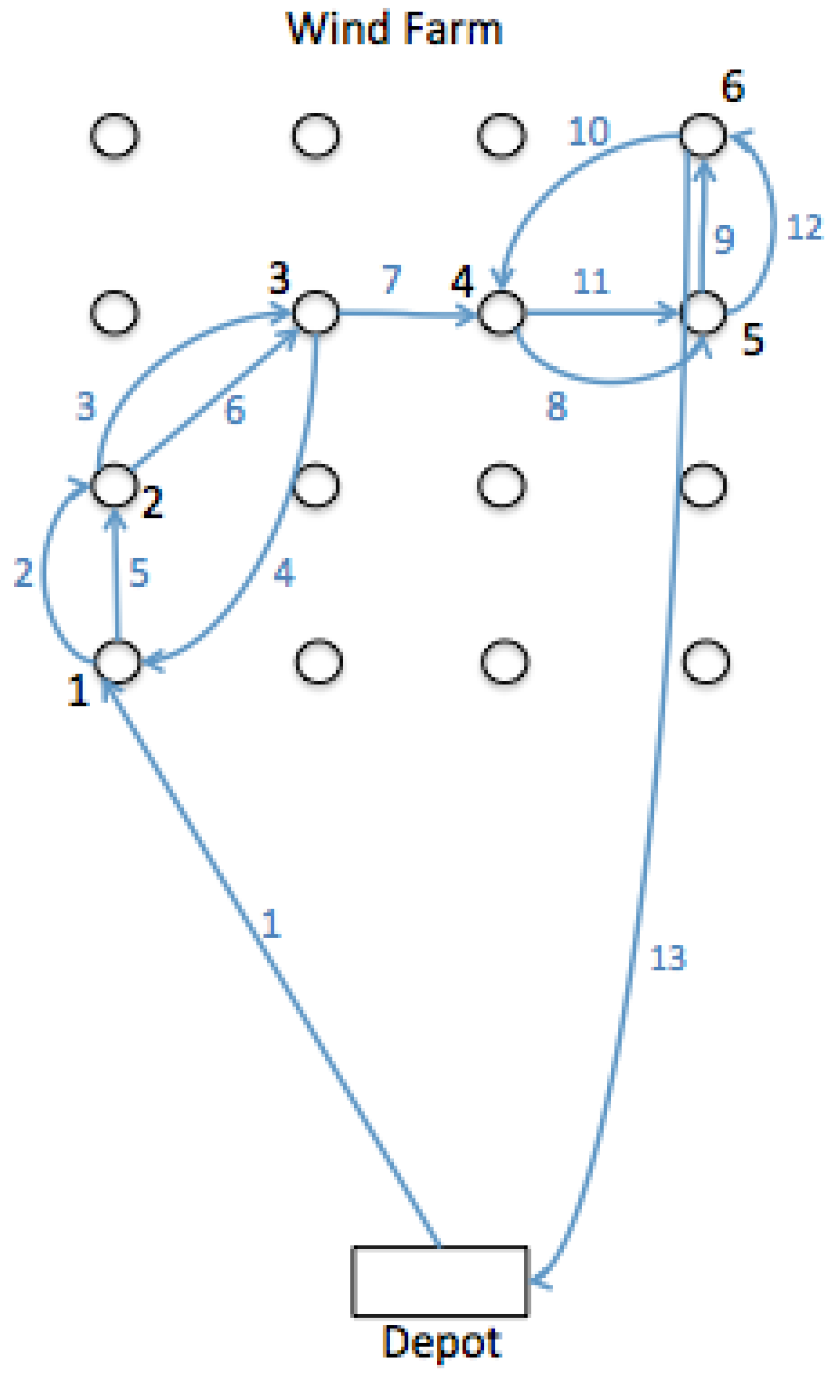
Maintenance tasks can be executed in parallel. This means that a vessel can leave technicians at turbines while delivering other technicians to different turbines. After working on the task for the scheduled amount of time, the technicians are picked up by the same vessel. Figure 1 illustrates the operations of a single vessel during a single shift, showing how the vessel ambulates between six different turbines to perform maintenance. Some tasks require the vessel to stay at the turbine, for example when needing more extensive equipment or when tasks involve sub-sea operations. The number of technicians required for different types of maintenance tasks is fixed, i.e., the number of technicians to perform a task cannot be increased to reduce the completion time of the task. It is also assumed that a technician crew belongs to one vessel, and the crew cannot be picked up by a different vessel during the shift.

The vessel fleet is given and consists of two different categories of vessels: Accommodation Vessels (AVs) and Crew Transfer Vessels (CTVs). Vessels vary in speed, fuel consumption, capacity, onboard equipment, and how often they need to return to the depot. All vessels may therefore not be compatible with all types of maintenance tasks. Vessels are also limited by weather conditions regarding when they can perform maintenance tasks, and these limits vary for different vessel types.

AVs and CTVs can leave the depot at most once during a shift. CTVs are required to return to the depot by the end of the shift, and they are not allowed to travel between wind farms. AVs can spend the time between shifts to travel between wind farms, thereby utilizing all the time in a shift to perform maintenance. However, travelling to or from the depot happens within shifts, as technicians can not leave the depot before their first shift starts or return after their last shift ends. AVs are required to return to the depot within a given number of shifts. They cannot leave the depot the same shift they return to the depot due to the time needed for preparations and loading of equipment and spare parts.

The scheduling of maintenance is affected by the weather conditions during the planning period, through the wind speeds and the wave conditions. The energy production, and therefore also the downtime costs, varies with the wind speed. The wind speed is taken as constant within a shift, hence, also the unit downtime cost for a turbine is fixed within a shift. The vessels have limitations on wave conditions for when they can transfer technicians to and from turbines, making the availability of the wind turbines dependent on the weather. The time slots within a shift when weather conditions are suitable for a vessel to transfer technicians to the turbine and perform maintenance are defined as weather windows. Factors that can influence these weather windows are wave heights, wave periods, wave directions, swell, currents, and wind speeds, in combination with the capabilities of a given vessel. A CTV can only leave the depot during a shift if its weather window during the shift is sufficiently long. Only one weather window is defined for each shift for each vessel. The weather forecast for the current time period is known when planning the schedules, as forecasting models have been developed to predict the wind speeds up till seven days ahead [32].

3. Mathematical Model

This section presents a mathematical model optimizing the routing and scheduling decisions when planning maintenance operations at offshore wind farms. The problem is a static and deterministic routing and scheduling problem. A short planning period is discretized into shorter time steps (shifts). The model outputs maintenance schedules for each shift in the planning period.

There are two levels of routing in the model, where the first level is routing of maintenance vessels between the depot and the wind farms. The problem is considered as a graph, where the depot and the wind farms are called nodes. The depot is represented by two nodes, a start depot node where each vessel starts a route, and a end depot node where the routes end. If a CTV stays in the depot during a shift, it is routed directly from the start depot node to the end depot node. The arcs between the nodes are associated to both travelling times and travelling costs.

The second level of routing consists of routing vessels between turbines that requires maintenance within a wind farm. The turbines requiring maintenance are represented by maintenance tasks. To simplify the model, the location of the turbines within a wind farm is ignored, and the travel times between each pair of turbines are considered equal: The distance between the turbines are considered negligible compared to the distance between nodes. To capture the time needed to travel between tasks and the related costs, an average internal transport time and transport cost are used instead.

Each turbine requiring maintenance is represented by two tasks, one delivery task and one pick-up task. As vessels can perform maintenance in parallel, technicians needs to be both dropped of at the turbine and then later picked up. The delivery task represents the beginning of the maintenance and the pick-up represents that technicians return to their vessel.

The model is designed to allow for some flexibility in the number of preventive tasks to be performed. There are more preventive tasks available than the target amount of preventive tasks to be completed. This is to allow for performing more preventive maintenance when the energy production is low. There is a distinction between performing a task and completing a task. Performing a task during a shift means working on the task during this shift, independent of whether the task is finished or not this shift. Completing a task during a shift means finishing the task during this shift.

In the following, lower-case letters are used to represent variables and indices, and capital letters are used to represent sets, constants, and used as superscripts to differentiate between sets and constants with otherwise equal names.

Indices

i,j	Nodes
m,n,l	Maintenance tasks
k	Type of maintenance tasks
v	Vessels
s	Shifts

Sets

$N^W$	All wind farm nodes, $N^W=\{1,2,\cdots ,|N^W\left|\right\}$, $N^W\subset N$
N	All nodes, $N=\{0,1,2,\cdots ,(|N^W|+1)\}$. Nodes $i\in \{1,2,\cdots ,|N^W\left|\right\}$ are wind farms and nodes $i\in \{0,(|N^W|+1)\}$ are the depot
K	All maintenance task types
M	All maintenance tasks including both delivery tasks and pick-up tasks, $M=\{0,1,2,\cdots ,|M\left|\right\}$
$M^{-}$	All delivery tasks (representing the actual maintenance tasks), $M^{-}=\{1,2,\cdots ,|M^{-}\left|\right\}$, $M^{-}\subset M$
$M_i^{-}$	All delivery tasks at wind farm i, $i\in N^W$, $M_i^{-}\subseteq M^{-}$
$M_{ik}^{-}$	All delivery tasks of type k at wind farm i, $i\in N^W$, $k\in K$, $M_{ik}^{-}\subseteq M_i^{-}$
$M^{+}$	All pick-up tasks $M^{+}=\left\{\right(|M^{-}|+1),\left(\right|M^{-}|+2),\cdots ,\left(2\right|M^{-}\left|\right)\}$, $M^{+}\subset M$
$M_i^{+}$	All pick-up tasks at wind farm i, $i\in N^W$, $M_i^{+}\subseteq M^{+}$
$M^C$	All corrective maintenance tasks, $M^C\subseteq M^{-}$
$M^P$	All preventive maintenance tasks, $M^P\subseteq M^{-}$
V	All vessels
$V^A$	All AVs, $V^A\subseteq V$
$V^C$	All CTVs, $V^C\subseteq V$
$V_m$	All vessels that can perform maintenance task m, $V_m\subseteq V$
$V_m^A$	All AVs that can perform maintenance task m, $V_m^A=V_m\cap V^A$
$V_m^C$	All CTVs that can perform maintenance task m, $V_m^C=V_m\cap V^C$
S	All shifts of the planning period
$S^0$	All shifts of the planning period, including the last shift of the previous planning period, shift 0

Constants

$T_{ijv}^T$	Transportation time between node $i\in N$ and node $j\in N$ for vessel $v\in V$
$T_m^{MT}$	Duration of task $m\in M^{-}$
$T^{PD}$	Time to transfer technicians from vessel to turbine and from turbine to vessel (transfer time)
$T_{iv}^{IT}$	Average time to travel between turbines in wind farm $i\in N^W$ for vessel $v\in V$
$D_v^{START}$	Number of shifts a vessel $v\in V^A$ has been offshore when the planning period starts
$D_v^{LIMIT}$	Number of shifts a vessel $v\in V^A$ can stay offshore without returning to the depot
$P_{iv}^{START}$	1 if vessel $v\in V^A$ is located at node $i\in N$ at the start of the planning period, 0 otherwise
$T^{DAY}$	Number of time units in a day
$T_s^{SHIFT}$	Length of shift $s\in S$
$T^{MIN}$	Minimum length of weather window in a shift for a CTV to leave the depot during the shift
$L_{vs}^W$	Lower bound for the weather window of vessel $v\in V$ in shift $s\in S$
$U_{vs}^W$	Upper bound for the weather window of vessel $v\in V$ in shift $s\in S$
B	The desired number of preventive maintenance tasks to be completed during the planning period
$R_{ms}$	1 if all necessary spare parts and equipment for performing task $m\in M^{-}$ are available in shift $s\in S$, 0 otherwise
$E_m$	1 if task m requires that the vessel performing the task is located at the turbine while the task is being performed, 0 otherwise
$Q_v$	Technician capacity of vessel $v\in V$
$P_m$	Number of technicians needed to perform task $m\in M$, positive for delivery tasks and negative for pick-up tasks
$C_{ijv}^T$	Transportation costs between node $i\in N$ and node $j\in N$ for vessel $v\in V$
$C_{ms}^{LP}$	Downtime costs per time unit during shift $s\in S$ due to loss of production when shutting down the turbine where maintenance task $m\in M^{-}$ is located
$C_v^{OUT}$	The cost for vessel $v\in V^A$ to stay offshore between two shifts
$C_v^{IT}$	The average internal transportation cost for vessel $v\in V$ to travel to a maintenance task $m\in M^{-}$ inside a wind farm
$C_m^{NP}$	The penalty cost per shift of not completing a preventive maintenance task during the planning period
$C_m^{NC}$	The penalty cost per shift of not completing a corrective maintenance task $m\in M^C$ during the planning period
$C_m^{NP\ast }$	The penalty cost per time unit of remaining work for a preventive maintenance task $m\in M^P$ that is not completed within the planning period
$C_m^{NC\ast }$	The penalty cost per time unit of remaining work for a corrective maintenance task $m\in M^C$ that is not completed within the planning period
$K_{ms}$	1 if the energy production during shift $s\in S$ is below a specified limit for when to perform $m\in M^{-}\cap M^P$ as extra preventive maintenance, 0 otherwise
δ	Small value greater than zero

Decision variables

$x_{mvs}$	1 if vessel $v\in V_m$ is used to perform maintenance task $m\in M$ during shift $s\in S$, 0 otherwise
$y_{ijvs}$	1 if vessel $v\in V$ travels directly between node $i\in N$ and $j\in N$, $i\ne j$, during shift $s\in S$, 0 otherwise
$z_{mnvs}$	1 if vessel $v\in V_m\cap V_n$ performs maintenance task $n\in M$ directly after maintenance task $m\in M$ during shift $s\in S$, 0 otherwise
$w_{ivs}$	1 if vessel $v\in V^A$ stays at node $i\in N$ between shift $s\in S$ and $(s+1)\in S$, 0 otherwise
$t_{mvs}$	The time vessel $v\in V_m$ starts maintenance task $m\in M$ during shift $s\in S$
$l_{ms}$	Time counter for how long the turbine where maintenance task $m\in M^{-}$ is located is shut down during shift $s\in S$. The time counter for shift s starts at 0 when the shift starts and reaches its maximum at the beginning of the next shift, $s+1$
$c_m$	The penalty cost of a task $m\in M^{-}$ that is not completed during the planning period
$p_{mvs}$	The number of technicians at vessel $v\in V_m$ immediately after visiting the turbine of task $m\in M$ during shift $s\in S$
$f_{ms}$	1 if task $m\in M^{-}$ is completed before the end of shift $s\in S$ (during shift s or during earlier shifts than s), 0 otherwise

Objective function

$$\begin{array}{cc}\mathrm{Min}\mathrm{Z}=\hfill & \sum _{i\in N}\sum _{j\in N}\sum _{v\in V}\sum _{s\in S}{C}_{ijv}^T{y}_{ijvs},\hfill \end{array}$$

(1a)

$$\begin{array}{c}+\sum _{m\in M^{-}}\sum _{v\in V_m}\sum _{s\in S}{C}_v^{IT}{x}_{mvs},\hfill \end{array}$$

(1b)

$$\begin{array}{c}+\sum _{i\in N^W}\sum _{v\in V^A}\sum _{s\in S}{C}_v^{OUT}{w}_{ivs},\hfill \end{array}$$

(1c)

$$\begin{array}{c}+\sum _{m\in M^{-}}\sum _{s\in S}{C}_{ms}^{LP}{l}_{ms},\hfill \end{array}$$

(1d)

$$\begin{array}{c}+\sum _{m\in M^C}\sum _{s\in S}{C}_m^{NC}(1-f_{ms}),\hfill \end{array}$$

(1e)

$$\begin{array}{c}+\sum _{m\in M^P}\sum _{s\in S}{C}_m^{NP}(1-f_{ms}),\hfill \end{array}$$

(1f)

$$\begin{array}{c}+\sum _{m\in M^{-}}{c}_m\hfill \end{array}$$

(1g)

The objective function aims to minimize the total costs of the problem. This includes both real costs and penalty costs. The real costs of the problem are represented by part (1a)–(1d). Part (1a) represents the transportation costs for the vessels between the depot and the wind farms, while part (1b) represents the internal transportation costs within a wind farm. Part (1c) represents the costs for AVs to stay offshore between shifts, i.e., night costs, and part (1d) represents the downtime costs.

Penalty costs are introduced to give incentives to perform tasks, and are represented by part (1e)–(1g). Part (1e) and part (1f) are penalty costs for not completing a task during a shift, where (1e) applies for corrective tasks and (1f) for preventive tasks. These parts make sure that the respective tasks are performed within a shift if there is free vessel capacity. There is also an incentive to work on tasks for which there is insufficient time to complete during the planning period, if there is free vessel capacity. Part (1g) gives a penalty cost for each task that is not completed based on how much time there is left of the task at the end of the planning period.

The constraints are grouped in constraints concerning flow of CTVs, flow of AVs, execution of tasks, time management, precedence of tasks, downtime, technicians balances and the domain of the decision variables.

Constraints for the flow of CTVs:

$$\begin{array}{ccc}\sum _{j\in N}{y}_{0jvs}=1,\hfill & & v\in V^C,s\in S,\hfill \end{array}$$

(2)

$$\begin{array}{ccc}\sum _{i\in N}{y}_{i\left|N\right|vs}=1,\hfill & & v\in V^C,s\in S,\hfill \end{array}$$

(3)

$$\begin{array}{ccc}{y}_{0\left|N\right|vs}=1,\hfill & & v\in V^C,s\in S|(U_{vs}^W-L_{vs}^W)<T^{MIN},\hfill \end{array}$$

(4)

$$\begin{array}{ccc}\sum _{i\in N}{y}_{ijvs}=\sum _{i\in N}{y}_{jivs},\hfill & & j\in N^W,v\in V^C,s\in S,\hfill \end{array}$$

(5)

$$\begin{array}{ccc}\sum _{i\in N}\sum _{j\in N}{y}_{ijvs}\le 2,\hfill & & v\in V^C,s\in S.\hfill \end{array}$$

(6)

All CTVs must during each shift leave the start depot node, $i=0$, and arrive at the end depot node, $i=\left|N\right|$. This is ensured by Constraints (2) and (3). Constraint (4) prevents that a CTV leaves the depot during a shift where the weather window for this vessel is shorter than a specified minimum requirement. Constraint (5) conserves node flow for CTVs by ensuring that when a CTV visits a wind farm node during a shift, it also leaves the node during the same shift. As CTVs cannot travel between wind farms during shifts, they can travel at maximum twice during each shift. This is restricted by Constraint (6).

Constraints for the flow of AVs:

$$\begin{array}{ccc}{w}_{iv(s-1)}+\sum _{j\in N}{y}_{jivs}=\sum _{j\in N}{y}_{ijvs}+w_{ivs},\hfill & & i\in N^W,v\in V^A,\hfill \\ & & s\in S^0\setminus \left\{0\right\},\hfill \end{array}$$

(7)

$$\begin{array}{ccc}\sum _{j\in N}{y}_{0jvs}=w_{\left|N\right|v(s-1)},\hfill & & v\in V^A,s\in S^0\setminus \left\{0\right\},\hfill \end{array}$$

(8)

$$\begin{array}{ccc}{w}_{\left|N\right|vs}=\sum _{j\in N}{y}_{j\left|N\right|vs},\hfill & & v\in V^A,s\in S.\hfill \end{array}$$

(9)

Constraint (7) conserves node flow for AVs. If an AV is located at a wind farm at the beginning of a shift, it either has to depart from this wind farm at the end of this shift or stay at this wind farm until the next shift. Constraints (8) and (9) conserve node flow for AVs to and from the depot node. An AV can only leave the depot during a shift if it was located at the depot at the end of the previous shift, which is ensured by Constraint (8). Constraint (9) ensures that $w_{\left|N\right|vs}$ shows that vessel v is situated in the depot at the end of the shift if v travels to the depot during shift s.

$$\begin{array}{ccc}\sum _{i\in N}\sum _{j\in N}{y}_{ijvs}\le 1,\hfill & & v\in V^A,s\in S,\hfill \end{array}$$

(10)

$$\begin{array}{ccc}{w}_{iv0}=P_{iv}^{START},\hfill & & i\in N,v\in V^A,\hfill \end{array}$$

(11)

$$\begin{array}{ccc}\sum _{i\in N^W}\sum _{s=1}^{D_v^{LIMIT}-D_v^{START}}{y}_{i\left|N\right|vs}\ge 1,\hfill & & v\in V^A\hfill \\ & & \mid D_v^{LIMIT}-D_v^{START}\le \left|S\right|.\hfill \end{array}$$

(12)

Constraint (10) prevents an AV from doing more than one trip during or prior to each shift. Where the AVs are located when the planning period starts are given by Constraint (11). While Constraint (12) ensures that the AVs do not stay offshore for longer than a specified allowed limit.

Constraints for the execution of tasks:

$$\begin{array}{ccc}\sum _{v\in V_m}{x}_{mvs}\le 1,\hfill & & m\in M^{-},s\in S,\hfill \end{array}$$

(13)

$$\begin{array}{ccc}{x}_{mvs}=1,\hfill & & v\in V^C,m=0\cup \left|M\right|,\hfill \\ & & s\in S,\hfill \end{array}$$

(14)

$$\begin{array}{ccc}{x}_{0vs}=w_{\left|N\right|v(s-1)},\hfill & & v\in V^A,s\in S^0|s>0,\hfill \end{array}$$

(15)

$$\begin{array}{ccc}{x}_{\left|M\right|vs}=w_{\left|N\right|vs},\hfill & & v\in V^A,s\in S,\hfill \end{array}$$

(16)

$$\begin{array}{ccc}{x}_{mvs}\le \sum _{j\in N}{y}_{jivs},\hfill & & i\in N^W,m\in M_i^{-}\cup M_i^{+},\hfill \\ & & v\in V_m^C,s\in S,\hfill \end{array}$$

(17)

$$\begin{array}{ccc}{x}_{mvs}\le \sum _{j\in N}{y}_{jivs}+w_{iv(s-1)}-\sum _{j\in N}{y}_{ijvs},\hfill & & i\in N^W,m\in M_i^{-}\cup M_i^{+},\hfill \\ & & v\in V_m^C,s\in S.\hfill \end{array}$$

(18)

Tasks can be performed by maximum one vessel each shift and this is ensured by Constraint (13). As CTVs start each shift in the depot, Constraint (14) forces the CTVs to perform the depot task in each shift. For AVs, the depot task should only be performed if the AVs are located at the depot during the shift. This is handled by Constraint (15) for the start depot task and Constraint (16) for the end depot task. A maintenance task at wind farm i can only be performed by a vessel that is located at this wind farm for the specified shift. This is restricted by Constraints (17) and (18) for CTVs and AVs, respectively.

$$\begin{array}{ccc}{x}_{mvs}=x_{(m+|M^{-}\left|\right)vs},\hfill & & m\in M^{-},v\in V_m,s\in S,\hfill \end{array}$$

(19)

$$\begin{array}{ccc}\sum _{v\in V_m}{x}_{mvs}=0,\hfill & & m\in M^{-},s\in S|R_{ms}=0,\hfill \end{array}$$

(20)

$$\begin{array}{ccc}\sum _{m\in M^P}\sum _{v\in V_m}{x}_{mvs}\le B,\hfill & & s\in S|K_{ms}=0.\hfill \end{array}$$

(21)

Constraint (19) makes sure that the delivery task and pick-up task at the same turbine are performed by the same vessel. Performing tasks that cannot be performed until a specified shift during the planning period are restricted by Constraint (20). They ensure that a task is not performed during a shift if the task is not ready to be performed this shift. For shifts where the energy production is higher than a specified limit, Constraint (21) ensures that the number of preventive tasks performed this shift does not exceed the desired number of preventive tasks to be performed during a shift.

$$\begin{array}{ccc}{T}_m^{MT}-\sum _{v\in V_m}\sum _{h=1}^s(t_{(m+|M^{-}|)vh}-t_{mvh}-T^{PD}{x}_{mvh})\hfill & & m\in M^{-},\hfill \\ +(T_s^{SHIFT}-T^{PD})f_{ms}\ge \delta ,\hfill & & s\in S,\hfill \end{array}$$

(22)

$$\begin{array}{ccc}\sum _{v\in V_m}\sum _{h=1}^s(t_{(m+|M^{-}|)vh}-t_{mvh}-T^{PD}{x}_{mvh})\hfill & & m\in M^{-},\hfill \\ \ge T_m^{MT}{f}_{ms},\hfill & & s\in S,\hfill \end{array}$$

(23)

$$\begin{array}{ccc}\sum _{v\in V_m}{x}_{mvs}\le 1-f_{m(s-1)},\hfill & & m\in M^{-},\hfill \\ & & s\in S\setminus \left\{1\right\}.\hfill \end{array}$$

(24)

Constraints (22)–(24) concern the variables that indicate in which shifts each task is completed. Constraint (22) forces $f_{ms}$ to one if task m is completed within shift s and Constraint (23) forces $f_{ms}$ to zero if task m is not completed within shift s. Constraint (24) prohibits that a task m is performed during shifts after the task is completed.

$$\begin{array}{c}\hfill c_m\ge C_m^{NC\ast }(T_m^{MT}-\sum _{v\in V_m}\sum _{s\in S}(t_{(m+|M^{-}|)vs}-t_{mvs}-T_m^{PD}{x}_{mvs})),\\ \hfill m\in M^C\cap M^{-},\end{array}$$

(25)

$$\begin{array}{c}\hfill c_m\ge C_m^{NP\ast }(T_m^{MT}-\sum _{v\in V_m}\sum _{s\in S}(t_{(m+|M^{-}|)vs}-t_{mvs}-T_m^{PD}{x}_{mvs}),\\ \hfill m\in M^P\cap M^{-}.\end{array}$$

(26)

Constraints (25) and (26) give incentive to work on tasks that are not completed during the planning period. If task m is completed, then $c_m$ is given the value of zero. If it is not completed, $c_m$ is equal to a penalty cost parameter multiplied with how much time is left of the task. Corrective tasks are given incentive by Constraint (25) and preventive tasks are given incentive by Constraint (26).

Constraints for the time management:

$$\begin{array}{ccc}{t}_{mvs}\le T^{SHIFT}{x}_{mvs},\hfill & & m\in M,v\in V_m,\hfill \\ & & s\in S,\hfill \end{array}$$

(27)

$$\begin{array}{ccc}{t}_{mvs}\ge L_{vs}^W\sum _{j\in N}{y}_{jivs}-T_s^{SHIFT}(1-x_{mvs}),\hfill & & i\in N^W,m\in M_i^{-},\hfill \\ & & v\in V_m^C,s\in S,\hfill \end{array}$$

(28)

$$\begin{array}{ccc}{t}_{mvs}\ge \sum _{j\in N}{T}_{jiv}^T{y}_{jivs}-T_s^{SHIFT}(1-x_{mvs}),\hfill & & i\in N^W,m\in M_i^{-},\hfill \\ & & v\in V_m^C,s\in S,\hfill \end{array}$$

(29)

$$\begin{array}{ccc}{t}_{mvs}\ge L_{vs}^W(\sum _{j\in N}{y}_{jivs}+w_{iv(s-1)})\hfill & & i\in N^W,m\in M_i^{-},\hfill \\ -T_s^{SHIFT}(1-x_{mvs}),\hfill & & v\in V_m^A,s\in S,\hfill \end{array}$$

(30)

$$\begin{array}{ccc}{t}_{mvs}\ge \sum _{j\in N^W}{T}_{0iv}^T{y}_{0ivs}-T_s^{SHIFT}(1-x_{mvs}),\hfill & & i\in N^W,m\in M_i^{-},\hfill \\ & & v\in V_m^A,s\in S,\hfill \end{array}$$

(31)

$$\begin{array}{ccc}{t}_{mvs}+T^{PD}{x}_{mvs}\le U_{vs}^W,\hfill & & m\in M^{+},v\in V_m,\hfill \\ & & s\in S.\hfill \end{array}$$

(32)

Constraint (27) forces the delivery and pick-up start times of tasks that are not performed to zero. For tasks that are performed, the start times of the delivery tasks are handled by Constraints (28)–(31). For tasks performed by CTVs, start times of the delivery tasks must both be higher than the lower bound of the weather windows and the transportation time from the depot to the wind farms. This is ensured by Constraints (28) and (29). The start time of delivery tasks performed by AVs must also be higher than the lower bound of the weather windows, which is ensured by Constraint (30). The start time of delivery tasks performed by AVs are only restricted by transportation time during shifts where the AVs leave the depot. This is because AVs travel between shifts when they travel between wind farms. This is not the case when AVs travels from or to the depot as this has to happen within the start and end shift of the technicians, respectively. Constraint (31) ensures that if an AV leaves the depot during a shift, it cannot start performing tasks before it has arrived at a wind farm. Constraint (32) makes sure that all pick-up tasks are started so that there is time to transfer the technicians from the turbine to the vessel within the weather window.

$$\begin{array}{ccc}{t}_{(m+|M^{-}\left|\right)vs}\ge t_{mvs}+T^{PD}{x}_{mvs},\hfill & & m\in M^{-},v\in V_m,s\in S,\hfill \end{array}$$

(33)

$$\begin{array}{ccc}{t}_{mvs}-t_{nvs}+T_{iv}^{IT}+T^{PD}\hfill & & i\in N^W,m\in M\setminus \left\{\right|M\left|\right\},\hfill \\ \le T_s^{SHIFT}(1-z_{mnvs}),\hfill & & n\in M_i^{-}\cup M_i^{+},v\in V_m\cap V_n,\hfill \\ & & s\in S|m\ne n,\hfill \end{array}$$

(34)

$$\begin{array}{ccc}{t}_{mvs}-t_{\left|M\right|vs}+T^{PD}{x}_{mvs}+T_{i\left|N\right|v}^T{y}_{i\left|N\right|vs}\hfill & & i\in N^W,m\in M_i^{-}\cup M_i^{+},\hfill \\ \le T_s^{SHIFT}(1-z_{m\left|M\right|vs}),\hfill & & v\in V_m\cap V_n,s\in S.\hfill \end{array}$$

(35)

A delivery task must be performed before the corresponding pick-up task, and the pick-up task cannot start before the technicians are transferred from the vessel to the turbine. This is ensured by Constraint (33). The start times of tasks are also restricted by the order in which the tasks are performed. Constraint (34) forces the start time of task n to be greater than the start time of task m plus the time for pick up and delivery and internal travel, if task m is performed directly before task n.

Constraint (34) also ensures that if an AV does not travel back to the depot during a shift, then the AV will have time to transfer the technicians from the last pick-up task it performs during the shift and travel out of the wind farm within the shift. The travel time of leaving a wind farm is set equal to the average internal travel time of the wind farm. Constraint (35) is a special case of Constraint (34) for tasks being performed directly before the end depot task. They always apply for CTVs, but for AVs they only apply for shifts where the AVs return to the depot. Constraint (35) makes sure that all pick-up tasks are started in time for the technicians to be transferred from the turbine to the vessel and for the vessel to return to the depot within the shift.

Constraints for the precedence of tasks:

$$\begin{array}{ccc}{x}_{mvs}=\sum _{n\in M\setminus \left\{0\right\}}{z}_{mnvs},\hfill & & m\in M\setminus \left\{\right|M\left|\right\},\hfill \\ & & v\in V_m^C\cap V_n^C,s\in S,\hfill \end{array}$$

(36)

$$\begin{array}{ccc}{x}_{mvs}=\sum _{n\in M\setminus \left\{\right|M\left|\right\}}{z}_{nmvs},\hfill & & m\in M\setminus \left\{0\right\},\hfill \\ & & v\in V_m^C\cap V_n^C,s\in S,\hfill \end{array}$$

(37)

$$\begin{array}{ccc}{x}_{mvs}\ge \sum _{n\in M\setminus \left\{0\right\}}{z}_{mnvs},\hfill & & m\in M\setminus \left\{\right|M\left|\right\},\hfill \\ & & v\in V_m^A\cap V_n^A,s\in S,\hfill \end{array}$$

(38)

$$\begin{array}{ccc}{x}_{mvs}\ge \sum _{n\in M\setminus \left\{\right|M\left|\right\}}{z}_{nmvs},\hfill & & m\in M\setminus \left\{0\right\},\hfill \\ & & v\in V_m^A\cap V_n^A,s\in S,\hfill \end{array}$$

(39)

$$\begin{array}{ccc}\sum _{m\in M\setminus \left\{\right|M\left|\right\}}\sum _{n\in M\setminus \left\{0\right\}}{z}_{mnvs}\ge \sum _{m\in M}{x}_{mvs}-1,\hfill & & v\in V_m^A\cap V_n^A,s\in S,\hfill \end{array}$$

(40)

$$\begin{array}{ccc}{z}_{mnvs}=x_{mvs},\hfill & & m\in M^{-},n=m+\left|M^{-}\right|,\hfill \\ & & v\in V_m,s\in S\hfill \\ & & |E_m=1.\hfill \end{array}$$

(41)

Constraints (36)–(40) concern the precedence of tasks. Precedence of tasks is also handled by Constraints (33)–(35) as these constraints ensure that the start time of a task, m, that is performed immediately before another task, n, is lower than the start time of task n. For all tasks performed by a CTV, excluding the depot tasks, exactly one task must be performed directly before and directly after every task. Constraint (36) ensures that if task m is performed, exactly one task is performed directly after task m, and if task m is not performed zero tasks are performed directly after task m. Constraint (37) is equivalent for tasks performed directly before task m.

As AVs do not have to start and end at the depot each shift, tasks performed by AVs must be handled somewhat differently, and this is done by Constraints (38)–(40). If an AV does not start a shift in the depot, there will not be a task performed directly before the first task it performs during this shift. The same applies for the last task it performs during a shift if it does not end this shift in the depot. As it is not known in advance when solving the model which tasks that are performed first and last, Constraints (36) and (37) do not apply for AVs. It is, however, known that for each task maximum one task can be performed directly after and directly before this task. It is also known that for tasks not performed, zero tasks can be performed directly before or after these tasks. This is restricted by Constraints (38) and (39). Constraint (40) gives a lower limit on the number of $z_{mnvs}$ that get the value one for for $v\in V^A$. This number equals the number of tasks performed minus one.

Constraints (41) applies for tasks that require the vessel performing the task to stay by the turbine when the task is being performed. For these tasks, the pick-up task is forced to be performed directly after the delivery task if the delivery task is performed.

Constraints for the downtime:

$$\begin{array}{ccc}{l}_{ms}\ge T^{DAY}(1-f_{ms}),\hfill & & m\in M^C,s\in S,\hfill \end{array}$$

(42)

$$\begin{array}{ccc}{l}_{ms}\ge \sum _{v\in V_m}(t_{(m+|M^{-}|)vs}+T^{PD}{x}_{mvs})\hfill & & \\ -T_s^{SHIFT}(1-(f_{ms}-f_{m(s-1)})),\hfill & & m\in M^C,s\in S\setminus \left\{1\right\},\hfill \end{array}$$

(43)

$$\begin{array}{ccc}{l}_{ms}\ge \sum _{v\in V_m}(t_{(m+|M^{-}|)vs}+T^{PD}{x}_{mvs})\hfill & & \\ -T_s^{SHIFT}(1-f_{ms}),\hfill & & m\in M^C,s=1.\hfill \end{array}$$

(44)

For corrective tasks the turbines are shut down from the failure occurs to the task is completed. The time counter, $l_{ms}$, of corrective tasks therefore include the total hours from the planning period starts to the tasks are completed. Constraints (42)–(44) concern this time counter. If a task m is not completed within the end of shift s, then the time counter of shift s is given the value of the time from the start of shift s to the start of the next shift, shift $s+1$. This is ensured by Constraint (42). Constraint (43) applies to the shifts where the tasks are completed. The time counter is then given the value of the time the turbine can be turned on, which is when the technicians are transferred from the turbine to the vessel after the task is completed. Constraint (44) is a special case of Constraint (43) for tasks that are completed during the first shift.

$$\begin{array}{ccc}{l}_{ms}\ge \sum _{v\in V_m}(t_{(m+|M^{-}|)vs}+T^{PD}{x}_{mvs}-t_{mvs}),\hfill & & m\in M^P,s\in S,\hfill \end{array}$$

(45)

$$\begin{array}{ccc}\sum _{v\in V_m}(t_{(m+|M^{-}|)vs}+T^{PD}{x}_{mvs}-t_{mvs})\hfill & & \\ \ge T^{MIN}{x}_{mvs},\hfill & & m\in M^P,s\in S.\hfill \end{array}$$

(46)

For preventive tasks, the turbines are shut down only during the performance of the tasks. It starts when a vessel arrives at the turbine and transfers technicians to the turbine, and ends when the technicians have returned to the vessel after performing the task. Constraint (45) gives value to the time counter for shifts that preventive tasks are performed. To avoid that technicians are left at a turbine for a time period that is so short that they in reality do not have time to perform any maintenance, Constraint (46) ensures that preventive maintenance must be performed continuous for a minimum amount of time.

Constraints for the balance of technicians:

$$\begin{array}{ccc}{z}_{mnvs}(p_{mvs}-P_n-p_{nvs})=0,\hfill & & m\in M\setminus \left\{\right|M\left|\right\},n\in M\setminus \left\{0\right\},\hfill \\ & & v\in V_m\cap V_n,s\in S,\hfill \end{array}$$

(47)

$$\begin{array}{ccc}{p}_{mvs}-P_n-p_{nvs}\le (Q_v-P_n)(1-z_{mnvs}),\hfill & & m\in M\setminus \left\{\right|M\left|\right\},n\in M\setminus \left\{0\right\},\hfill \\ & & v\in V_m\cap V_n,s\in S,\hfill \end{array}$$

(48)

$$\begin{array}{ccc}{p}_{mvs}-P_n-p_{nvs}\ge (-P_n-Q_v)(1-z_{mnvs}),\hfill & & m\in M\setminus \left\{\right|M\left|\right\},n\in M\setminus \left\{0\right\},\hfill \\ & & v\in V_m\cap V_n,s\in S.\hfill \end{array}$$

(49)

The technician flow for each task is handled by Constraint (47). These constraints ensure that if task n is performed directly after task m by vessel v, then the number of technicians onboard vessel v after visiting task n must be equal to the number of technicians onboard vessel v after visiting task m and the technicians leaving or entering the turbine of task n. The demand for delivery tasks is positive and the demand for pick-up tasks is negative. Constraint (47) is non-linear and is linearized by replacing it with Constraints (48) and (49).

$$\begin{array}{ccc}{p}_{mvs}\le (Q_v-P_m)x_{mvs},\hfill & & m\in M^{-},v\in V_m,s\in S,\hfill \end{array}$$

(50)

$$\begin{array}{ccc}{p}_{mvs}\le Q_v{x}_{mvs},\hfill & & m\in M^{+},v\in V_m,s\in S,\hfill \end{array}$$

(51)

$$\begin{array}{ccc}{p}_{mvs}\ge -P_m{x}_{mvs},\hfill & & m\in M^{+},v\in V_m,s\in S,\hfill \end{array}$$

(52)

$$\begin{array}{ccc}{p}_{mvs}\le Q_v{x}_{mvs},\hfill & & m=\left\{0\right\}\cup m=\left\{\right|M\left|\right\},\hfill \\ & & v\in V_m,s\in S.\hfill \end{array}$$

(53)

$$\begin{array}{ccc}{p}_{mvs}\ge (Q_v-P_m)x_{mvs},\hfill & & m\in M^{-},v\in V_m,\hfill \\ & & s\in S|E_m=1,\hfill \end{array}$$

(54)

Constraints (50)–(53) handle the technician capacity of the vessels for delivery, pick-up and depot tasks. When a vessel is performing a task m that requires the vessel to stay by the turbine, the vessel are not allowed to have other technicians performing tasks in parallel at other turbines. This is prevented by Constraint (54), together with Constraint (50). These constraints force the number of technicians onboard the vessel after performing task m to be equal to the capacity of the vessel minus the technician demand at task m. For these types of tasks, the pick-up task must be performed directly after the delivery task. This means that except for the technicians performing task m, all other technicians have to be onboard the vessel for the entire time task m is being performed.

The domains of the decision variables:

$$\begin{array}{ccc}{x}_{mvs}\in [0,1],\hfill & & m\in M,v\in V_m,s\in S,\hfill \end{array}$$

(55)

$$\begin{array}{ccc}{y}_{ijvs}\in [0,1],\hfill & & i,j\in N,v\in V,s\in S,i\ne j,\hfill \end{array}$$

(56)

$$\begin{array}{ccc}{z}_{mnvs}\in [0,1],\hfill & & i\in N^W,m,n\in M_i,v\in V_m\cap V_n,s\in S,\hfill \end{array}$$

(57)

$$\begin{array}{ccc}{w}_{ivs}\in [0,1],\hfill & & i\in N,v\in V^A,s\in S,\hfill \end{array}$$

(58)

$$\begin{array}{ccc}{f}_{mvs}\in [0,1]\hfill & & m\in M,v\in V_m,s\in S,\hfill \end{array}$$

(59)

$$\begin{array}{ccc}{t}_{mvs}\ge 0,\hfill & & m\in M,v\in V,s\in S,\hfill \end{array}$$

(60)

$$\begin{array}{ccc}{l}_{ms}\ge 0,\hfill & & m\in M,s\in S,\hfill \end{array}$$

(61)

$$\begin{array}{ccc}{p}_{mvs}\ge 0,integer\hfill & & m\in M,v\in V_m,s\in S,\hfill \end{array}$$

(62)

$$\begin{array}{ccc}{c}_m\ge 0,integer\hfill & & m\in M.\hfill \end{array}$$

(63)

The domain of the decision variables are defined by Constraints (55)–(63). In the supplemental material a small numerical example is provided to illustrate the model.

4. Solution Methods

The mathematical model presented in Section 3 is large and potentially time consuming to solve. It is trivial to find a feasible solution, as it is possible to let all vessels be idle, without performing any tasks. An optimal solution can in principle be found using commercial mixed integer programming (MIP) solvers, but the branch-and-bound search used in these solvers have a running time that increases exponentially with the number of binary and integer variables. Some instances of the model can therefore be solved directly using MIP solvers, whereas for larger instances we have developed two different rolling horizon heuristics [33]. Furthermore, we propose a set of symmetry breaking constraints that can be added to the model to remove many variable assignments that correspond to identical solutions, without changing the resulting optimal value.

4.1. Rolling Horizon Heuristics

Rolling horizon heuristics are used to iteratively produce solutions to MIPs by considering shorter sub-horizons of the planning horizon. Each sub-horizon is split into two time blocks, one detailed time block (DTB) and one aggregate time block (ATB). For each iteration k, the DTB is modelled in detail, while the ATB is simplified according to a simplification strategy and represented in an aggregate manner to evaluate the impact of future available capacity when solving for the DTB [33]. Before solving for the next iteration, $k+1$, some or all of the decisions made for the DTB are fixed according to a specified fixing strategy. These variables remain fixed for all subsequent iterations. The fixed part of the DTB are referred to as the fixed DTB, while the free variables of the DTB are referred to as the free DTB. For the next iteration, $k+1$, the DTB is expanded with a specified number of time periods so that the first part of $AT{B}_k$ becomes a part of $DT{B}_{k+1}$, and the $AT{B}_{k+1}$ is shifted towards the end of the planning period with an equal number of time periods. If the length of the planning period is equal to the combined length of the DTB and the ATB, then the length of the ATB decreases in each iteration [33]. The problem is solved when the entire planning period is included in, and solved for, the DTB. The fixed DTB, the free DTB and the ATB of a general rolling horizon heuristic are illustrated graphically by Figure 2.

Rolling horizon heuristics can reduce the computational requirements significantly, while still producing close to optimal solutions. The effectiveness of the heuristic is, however, highly dependent on the simplification strategy used for the ATB and fixing strategy used for the fixed DTB [33]. Two different rolling horizon heuristics, RHH-1 and RHH-2, are proposed for the problem studied here. The length of the free DTB is set to one shift and identical simplification strategies are implemented for both RHH-1 and RHH-2. As the planning period of the problem is relatively short, the length of the ATB is set equal to the remaining part of the planning period. All variables restricted to be binary or integer are replaced by continuous variables in the ATB. The two rolling horizon heuristics differ in which decisions are fixed in the DTB.

To account for the inaccuracies caused by variables that take fractional values, and to tighten the model formulation for the ATB, the redundant Constraint (64) is introduced in the rolling horizon heuristics. These constraints ensure that the total number of man-hours of maintenance performed in the planning period does not exceed the man-hour capacity of the vessel fleet for the planning period. To represent the total capacity of the vessel fleet, the parameter $W_{ivs}$ is introduced. This parameter equals the available number of hours in shift s that vessel v can perform maintenance in wind farm i. The number of available hours for the vessel fleet is then multiplied by the number of technicians in the vessel fleet to represent the total number of available man-hours. The $W_{ivs}$ parameter is adjusted for weather windows during shift s and transportation times to node i for vessel v. As transportation times for AVs are dependent on where the AVs are located during the respective shifts, the transportation times for AVs are not known when $W_{ivs}$ is calculated. The $W_{ivs}$ therefore gives an optimistic estimate of the total available hours for the vessel fleet to perform maintenance.

$$\begin{array}{c}\sum _{m\in M_i^{-}}{P}_m(t_{(m+|M^{-}|)vs}-t_{mvs}+T^{PD}{x}_{mvs})\le Q_v{W}_{ivs},\hfill \\ \hfill i\in N^W,v\in V,s\in S.& \end{array}$$

(64)

For both RHH-1 and RHH-2 only the decisions which positively indicate to perform tasks or to travel between nodes are fixed. That is, if a solution in one iteration suggests not to perform a specific task, the decision is not fixed. This is to prevent that good solutions that involve doing more than originally planned are prohibited in subsequent iterations.

In RHH-1, it is not allowed to remove any tasks from the schedules or change the order of existing tasks, but it is allowed to add new tasks to the schedules at later iterations. The vessels that should perform a given task is not fixed, but if a task is scheduled to be performed in shift s, then some vessel $u\in V_m$ has to perform it. If vessel v travels between two nodes i and j during shift s, then some vessel $u\in V_m$ must travel between node i and node j during shift s. If a task is scheduled to be completed during shift s, the decision can not be altered.

To allow for adding new tasks, but not to change the order of existing tasks, the $z_{mnvs}$-variables are fixed for tasks that are performed, but not performed in sequence. By keeping the $z_{mnvs}$-variables of tasks performed in sequence free, new tasks can be scheduled in between these tasks. As for the $x_{mvs}$-variables, the $z_{mnvs}$-variables are not fixed with respect to what specific vessel that performs the different sequences of tasks. To allow for additional tasks to be included for earlier shifts in later iterations, the variables $l_{ms}$, $t_{mvs}$ and $p_{mvs}$ are not fixed. As $l_{ms}$ and $t_{mvs}$ are not fixed, this opens up for the possibility to change the amount of time spent on maintenance tasks in later iterations. This does not increase the complexity of the heuristic significantly, as these variables are continuous in the DTB. The combination of the rules presented for RHH-1 also allows for AVs to be relocated during later iterations. As an AV constitutes a significant amount of the capacity of a vessel fleet, it could be unfortunate for the solution quality to, for example, fix an AV to the depot during a shift.

In RHH-2 most of the decisions regarding how the vessels move and which tasks they perform are fixed. The only decisions regarding vessels that are not fixed, are for vessels that are not scheduled to perform maintenance. This means that vessels that originally were scheduled not to perform maintenance can be re-scheduled in later iterations. Most of the decisions regarding scheduled tasks are fixed in RHH-2. Scheduled tasks cannot be removed from the schedules in later iterations, additional tasks cannot be scheduled in between scheduled tasks and the order of the tasks cannot be changed. However, tasks can be added at the beginning and at the end of the scheduled tasks. The $l_{ms}$- and $t_{mvs}$-variables are not fixed, which allows for the scheduled amount of time to perform each task to be changed in later iterations. Decisions regarding tasks that are not scheduled to be performed are not fixed, and these tasks are therefore in later iterations allowed to be scheduled to vessels that originally were scheduled not to perform maintenance, or at the beginning and the end of a schedule for a vessel already in the schedule. The mathematical formulation of the fixing strategies for RHH-1 and RHH-2 are provided in the supplemental material.

4.2. Symmetry Breaking Constraints

Symmetry in a problem is problematic as it increases the size of the search space. This can make it harder to prove optimality of the solutions of the problem and therefore increase the computational time. One way to reduce symmetry in a problem is to add symmetry breaking constraints in the model formulation. There can, however, be some problems associated to adding symmetry breaking constraints in heuristic methods. When adding these constraints particular solutions are eliminated, and this may conflict with the direction of the branching heuristics [34]. For the problem described here, symmetry is caused by tasks of the same type within the same wind farm and vessels of the same type. Tasks of the same type within a wind farm are assumed identical, and the same applies for vessels of the same type. Therefore, mathematically different solutions can exist that in practice refer to identical decisions. In the supplemental material of the paper we provide details of symmetry breaking constraints dictating that during each shift, tasks of lower task numbers must be performed before tasks of higher task numbers, for tasks of the same type within the same wind farm. If multiple vessels are located in the same wind farm, the vessels of lower indices must perform the tasks of lower indices as long as the tasks are of the same type.

5. Computational Study

A computational study was conducted to test the correctness of the model, as well as to (1) analyze the computational effort required to solve the model to optimality and heuristically using the rolling horizon heuristics; (2) analyze different modelling choices, such as the length of the planning horizon, with respect to the quality of solutions obtained from the perspective of solving a dynamic problem; and (3) show how the model can be used to evaluate strategic decisions such as fleet size and mix decisions.

The mathematical model and the rolling horizon heuristics were implemented using Xpress Mosel and solved using Xpress version 7.8.0. To enhance the chance of finding high quality solutions, the automatic strategies for cuts and heuristics in Xpress were overruled for the implementation of both the exact model and the heuristics. The cut strategy was set to no cuts, 0, to avoid spending unnecessary time to improve the bound and instead focus on finding better solutions. For the heuristic strategy, an extensive heuristic strategy was chosen. Using an extensive search, more time is allocated at the beginning of the solving process to finding a good solution. Simulations were implemented in MATLAB, version R2014a. The computational tests were performed on a HP DL 165 G6 computer with an AMD Opteron 2431 2,4 GHz processor, 24 GB of RAM and running on a Linux operating system.

The tests were conducted with instances created based in part on real data and in part on reasonable assumptions based on current best practice. The instances include three types of vessels: an AV, a regular CTV, and a type of CTV called SES (surface effect ship). We consider two wind farms located 50 kilometers apart, but vary the number of turbines in each wind farm. Instances consider six types of maintenance tasks: triggered alarms, manual resets, minor repairs, medium repairs, major repairs, and preventive maintenance. Various sources and expert opinions have been consulted to obtain realistic parameters for the instances, mainly based on a reference case created for verification of O&M simulation models for offshore wind farms by Dinwoodie et al. [35]. Additional sources have been used for data on the wave height limits of the different vessels [36,37], transportation costs [23] and daily cost rates [38], maintenance task categories and failure rates [39], and weather conditions [40]. Details on the data used to create the test instances are provided in the supplemental material.

Our computational experiments provided support for the correctness of the model, as illustrated through the small numerical example provided in the supplemental material. The following subsections present overall findings from our computational study, with respect to the computational effort required to solve the model and to use the rolling horizon heuristics, to the performance of the methods in a dynamic setting, and to the evaluation of strategic decisions regarding fleet sizing.

5.1. Evaluating Computational Effort

To assess the computational effort required to solve the model and to use the rolling horizon heuristics, instances with between 1 and 3 shifts were generated. A group of 20 different instances was generated for different numbers of turbines, in the range from 120 to 180 turbines. In all instances, the two wind farms were served by one AV and one SES, using 12 h shifts. We set a time limit of two hours (7200 s) for solving the model. For the heuristics, a time limit of 2000 s is set per iteration, thereby limiting the run times to less than 6000 s for instances with three shifts.

Our main results regarding the computational effort required to solve the model are presented in

Table 1. Test instances used to evaluate efficiency of full model, with results from using the full model and the RHH-2 heuristic with symmetry breaking constraints. For each group of instances, 20 random instances are generated with different maintenance tasks included.

Shifts, Turbines	Tasks	Full Model		RHH-2
		Feasible	Optimal	Feasible	Better
1, 120	8–17	20	9	NA	NA
1, 140	11–25	20	3	NA	NA
1, 160	11–23	20	3	NA	NA
1, 180	14–27	20	1	NA	NA
2, 120	8–17	14	8	20	17
2, 140	11–25	8	3	20	19
3, 120	8–17	17	8	20	14
3, 140	11–25	13	2	20	10
3, 160	11–23	10	0	17	13

. When solving the model directly, finding a proof of optimality within two hours is a challenge for the instances included in the test. For instances with 1 shift, the full model can be used to consistently find feasible solutions, and for problems with relatively few maintenance tasks, solutions can occasionally be proven optimal within two hours. For instances with two or more shifts, solving the full model does not always result in any feasible solution.

We also tested the two rolling horizon heuristics on the instances in Table 1 with more than one shift. The table shows only results for RHH-2 with symmetry breaking constraints included. The RHH-1 heuristic performs worse than RHH-2. Results are shown for the case with symmetry breaking constraints, as without those constraints the solution times increase and the method is not able to find feasible solutions to as many instances. Additional details of these tests are reported in the Supplementary Materials.

5.2. Performance in a Dynamic Setting

While the mathematical model covers decisions for several shifts, practical use of the model would entail to solve the model repeatedly as new information about corrective maintenance appears. In the following tests, all decisions are assumed to be taken before the start of each shift. New information regarding alarms and maintenance tasks that arrive during a shift is then incorporated into the planning for the next shift, together with updated weather forecasts and an updates on remaining maintenance tasks and vessel locations. We focus on using either the full model or the RHH-2 to make decisions for the upcoming shift, and test the effect of varying the length of the planning period, the number of iterations solved for a specific length of the planning period, and the upper limit on the solution time of each iteration in the heuristic.

For the tests of this section, a simulation period of seven shifts are used. The results of a simulation can be affected somewhat by some start and end effects of the simulation period. To minimize these effects, two measures are included to reduce start and end effects. Corrective tasks which symbolizes the result of checked alarms in the shift prior to the first shift of the simulation period are generated and included in the simulations. This is done to capture some of the decisions made in earlier periods and, which will reduce the start effects. To reduce the end effects of the simulations, input data (or information) of all shifts in the planning period of the last shift in the simulations are included. This means that if the length of the simulation period is n and the length of the planning period is $\left|S\right|$, then information on all shifts from shift 1 in the simulation period to shift $n+\left|S\right|-1$ is included in the simulations.

To evaluate the different aspects of the models studied in each test, solution time and solution quality are compared. Solution quality is evaluated based on real costs and the number of hours of maintenance performed. Daily fixed costs, such as daily vessel rates, are not included, as these occur for each shift regardless of the schedules generated. The number of hours of maintenance performed includes both corrective and preventive maintenance.

Changing the length of the planning period was tested to see if the value of additional information from including more shifts in the planning period improve the solution quality. To test the planning period length, ten simulation runs spanning seven days were executed for a case with 120 turbines, using planning periods of one, two, and three shifts, respectively. The RHH-2 heuristic was used to obtain solutions when using more than one shift in the planning horizon, and the full model was used for planning horizons of only one shift.

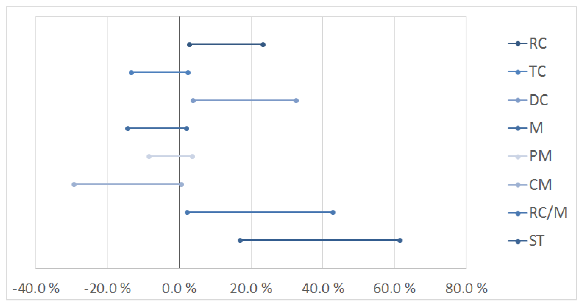
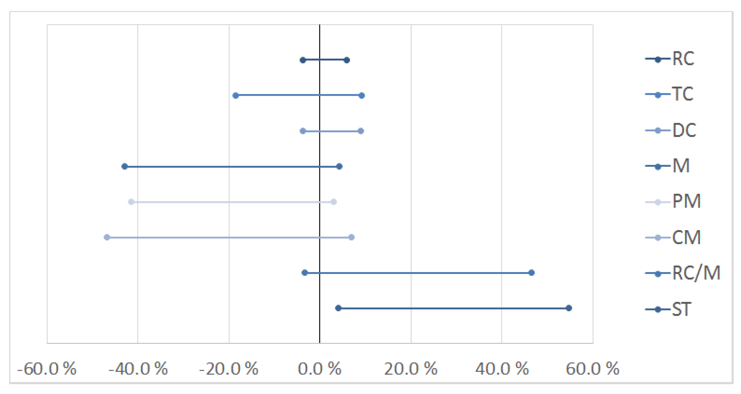
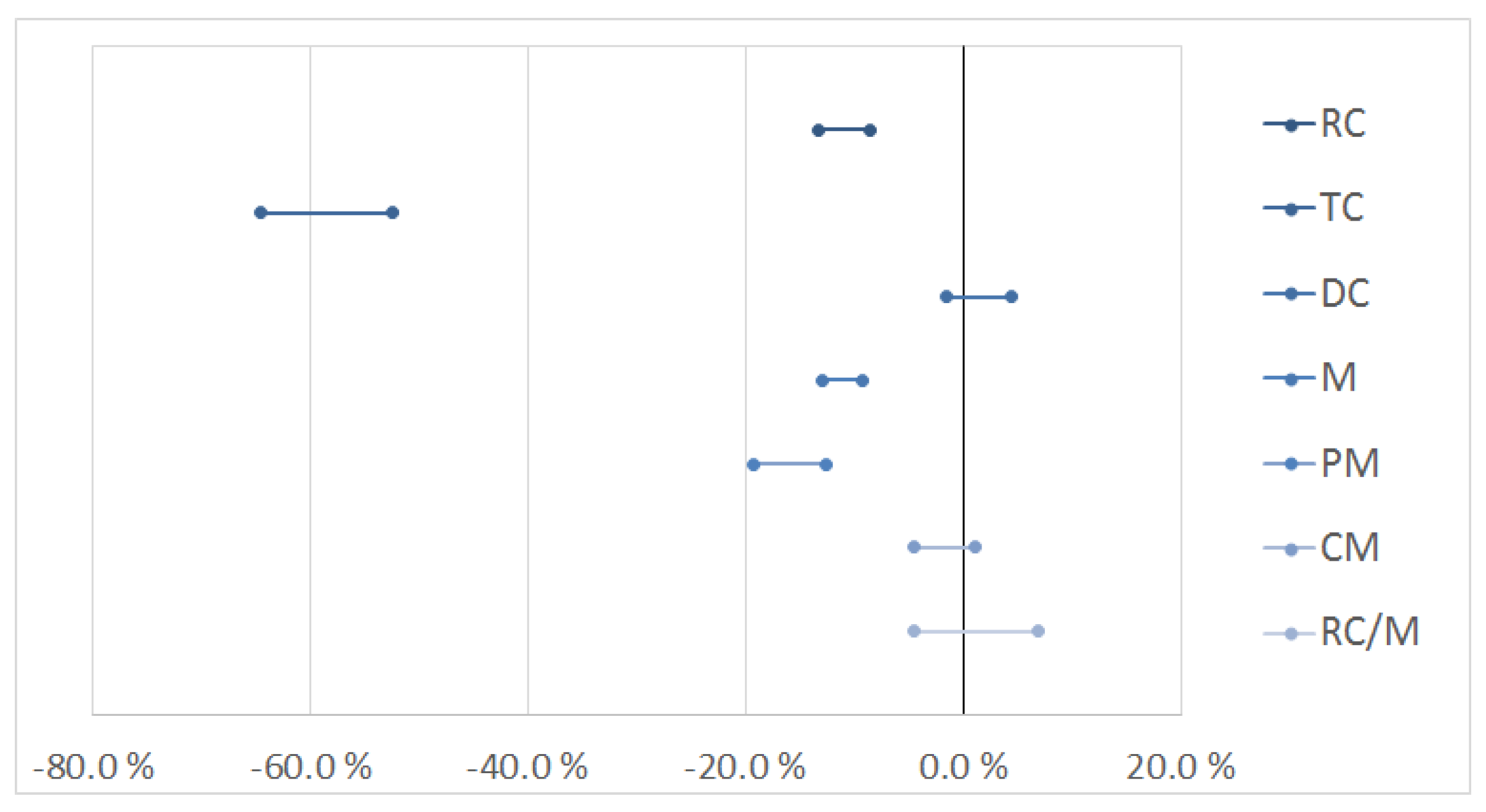
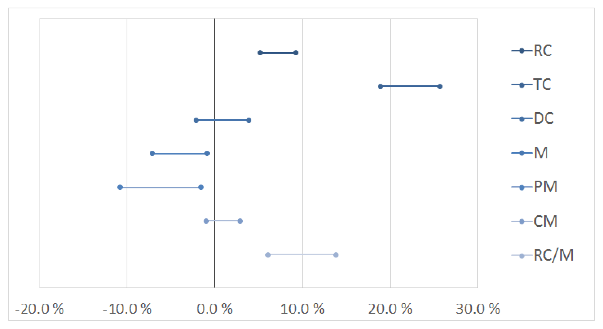
Figure 3 presents the results of comparing RHH-2 solved for planning periods of two and three shifts. The results of comparing RHH-2 solved for a planning period of two shifts and the exact model solved for one shift are presented in Figure 4. The upper time limit of the exact model is reduced to the time that is allocated to solve each iteration of the heuristic, to 2000 seconds. The abbreviations used in the figures are as follows. RC: real costs (artificial penalty costs not included), TC: transportation costs, DC: downtime costs, M: hours of maintenance, PM: hours of preventive maintenance, CM: hours of corrective maintenance, RC/M: real costs per hour of maintenance, ST: solution time.

The figures show that by reducing the length of the planning period, the solution time is reduced. This is especially due to reduction in the number of iterations. Reducing the length of the planning period also improves the solution quality, generally the real costs are reduced and more maintenance is performed. It appears that the heuristic puts too little emphasis on the first shift of the planning period and that it uses too much computational effort on solving later shifts. Reducing the length of the planning period therefore reduces the computational effort needed to solve the problem. These results imply that the value of including information on additional shifts in the planning period is lower than the decrease in solution quality caused by the extra computational effort needed, hence, a greedy approach is favorable for the problem studied here.

One of the reasons that the value of additional information of later shifts is limited can be that it is favorable to perform most maintenance task during the first shifts, regardless of the weather forecasts of later shifts. For corrective tasks this applies due to the running downtime costs; It is never more favorable to perform a corrective task in a later shift if there is enough capacity to perform it during the first shifts. As preventive tasks are of a relatively long duration and the penalty costs give incentives based on the hours of performed maintenance, it is also favorable to perform preventive tasks in earlier shifts, as long as the electricity production is lower than a specific limit.

Additional tests were executed to see if reducing the number of iterations in the RHH-2, and allowing more time per iteration, could improve the performance when including two shifts in the planning horizon. When the number of iterations in RHH-2 is reduced, the heuristic only gives integer feasible solutions for the shifts included in the detailed time blocks of the performed iterations, while the remaining shifts may still guide the solution process even though only continuous variables are used.

Simulation runs for the case with 120 turbines were considered, comparing the use of one or two iterations of RHH-2 for a planning horizon of two shifts. The results show that reducing the number of iterations for RHH-2 reduces the solution time, without worsening the simulated costs: with two iterations the downtime costs are found to be slightly lower and the transportation costs slightly higher, without being statistically significant. Compared to the exact model with one planning period, RHH-2 with one iteration reduces the solution time, however, the solution quality of the full model is significantly higher. The full model with one planning period is therefore also considered as better than RHH-2 with a planning period of two shifts solved for one iteration. Furthermore, tests were made in which the RHH-2 was allowed to run for 3600 s instead of 2000 s per iteration for planning horizons of two shifts. Comparing this to the use of the full model reveals that the difference in solution quality is not substantial, however, the full model provides slightly better solutions than RHH-2, while the solution time of the full model is significantly lower. We therefore conclude that in a dynamic setting, the best choice is to use the full model for a planning horizon of only one shift: even though longer planning horizons can be handled using the RHH-2, it seems that the end-of horizon effects are handled well in our mathematical model and that the artificial penalty costs are sufficient to select good maintenance tasks for execution when only planning for one shift.

5.3. Comparing Strategic Decisions

Simulations can provide valuable information when analyzing strategic aspects of O&M in offshore wind farms. The simulations can show how the different strategic decisions affect the performance on an operational level. To illustrate this, this section presents the results of analyzing the vessel fleet size and mix. The different strategic decisions are simulated for 14 shifts and their effect on the operational performance are compared in terms of real costs and hours of maintenance performed.

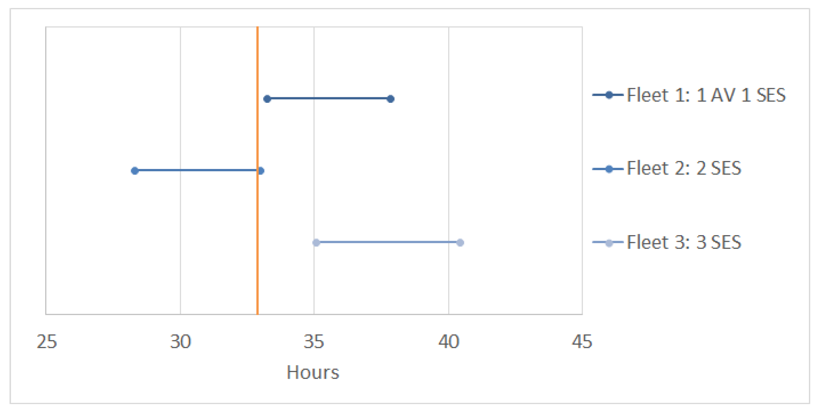
Three different vessel fleets were analyzed using ten simulation runs for a case with two wind farms and a total of 100 turbines. Fleet 1 consists of 1 AV and 1 SES, Fleet 2 consists of 2 SESes, and Fleet 3 consists of 3 SESs. The confidence intervals for the number of hours of preventive tasks performed for the ten simulation runs, for each of the three vessel fleets, are presented in Figure 5. The results indicate that the technician capacity of Fleet 1 and Fleet 3 is sufficient, as they both have capacity to perform more preventive maintenance than the average hours required during the simulation period in order to complete all yearly preventive tasks. Using Fleet 2, the number of hours of preventive maintenance is lower, suggesting that the technician capacity of Fleet 2 may be too small.

The effect of changing the fleet capacity by replacing an AV with a SES is further presented in Figure 6. AVs have twice the capacity of SESes and CTVs, and thus, an AV has a relatively large impact on the total technician capacity of the fleet. These results show that Fleet 2 performs better than Fleet 1 in terms of costs. This is linked to the higher transportation costs of Fleet 1, as AVs have significantly higher transportation costs than SESes. However, Fleet 2 has higher downtime costs. This is due to the fact that the lower capacity of vessel Fleet 2 causes some corrective maintenance tasks to be delayed until technicians are available, and the turbines are therefore shut down for a longer time period.

By comparing the capacity of Fleet 1 and Fleet 2 with the hours of maintenance they perform, it can be seen that while Fleet 1 has 1.5 times the capacity of Fleet 2, Fleet 1 only performs 10% to 15% more hours of maintenance. As seen in Figure 5, Fleet 1 performs sufficient preventive maintenance, and one reason that there is unused capacity in Fleet 1 can therefore be that Fleet 1 has overcapacity. Another reason for this unused capacity can be the relatively long time it takes to transfer technicians to and from the turbines, as this puts a limit on the number of maintenance tasks a vessel can perform during a shift. Fleet 1 is therefore compared to a third fleet, Fleet 3, that has equal technician capacity, but a larger limit on how many tasks can be performed during a shift, as it consists of an additional vessel.

The results of comparing Fleet 1 and Fleet 3 are presented in Figure 7. Even when adding an additional SES, the transportation costs of Fleet 1 are considerably higher than for fleets of only SESes. Fleet 3 performs more preventive maintenance than Fleet 1, which implies that the amount of maintenance performed by Fleet 1 is restricted by the limit on how many tasks that can be performed during a shift.

6. Concluding Remarks

Offshore wind energy production is growing, but is currently more expensive than onshore production. Higher maintenance costs are one of the reasons behind this difference, and it is therefore considered important to consider how to minimize the costs incurred by performing maintenance on offshore turbines. This paper presents a mathematical model that can be used for routing and scheduling of vessels to perform maintenance operations at offshore wind farms. Among the novel features of the mathematical model is (1) the inclusion of several wind farms at different locations; (2) covering several shifts in the planning horizon; and (3) modelling both CTVs and AVs.

To the authors knowledge, this is the first time that this problem has been considered in a dynamic setting, and we use simulations to evaluate solution methods developed to solve instances of the mathematical model. An unsuspected finding is that the value of modelling several periods appears to be negative: less efficient solutions are found with a longer planning horizon. This makes us believe that the end-of-horizon effects are handled efficiently in the mathematical model, and that the increased computational difficulty associated with a longer planning horizon results in a situation where it is more efficient to consider only one period when deciding on routes and schedules for maintenance vessels.

The results show the importance of evaluating a tactical decision support tool by simulation and not by the results when solving static models: When only considering a static situation, seeking to best utilize resources over a fixed time horizon, a rolling horizon heuristic outperformed the direct solution of the full mathematical model. However, when evaluated in a dynamic setting, the direct solution of the full model over a limited planning horizon gives better results.

We also illustrated how combining the mathematical model with simulations can be used to evaluate strategic decisions, such as determining an appropriate fleet size and mix. Another use would be to estimate the consequences of using separate fleets for different wind farms, as opposed to having a joint vessel fleet.

The amount of preventive maintenance that is scheduled depends on the value of different penalty parameters. These parameters depend on the particular application, and should be adjusted for different settings to fit the number of turbines, the vessel fleet, and the preventive maintenance strategy used by the wind farm operator. When embedded in simulations, the presented mathematical model may be used to analyze different strategies for scheduling preventive maintenance, which remains a difficult strategic issue for offshore wind farm operators.

Applying the model to a real case remains as future work. Most optimization models developed for scheduling of maintenance tasks and routing of vessels to perform those tasks have been focusing on strategic decisions, such as determining a suitable fleet composition. As more offshore wind farms are being put into operation, the need for tactical decision support will continue to grow.