Development of the Hydrodynamic Model for Long-Term Simulation of Water Quality Processes of the Tidal James River, Virginia

Abstract

Harmful algal blooms (HABs) have frequently occurred in the James River. The State has convened a Scientific Advisory Panel (SAP) to review the James River chlorophyll-a standards. The SAP will conduct a scientific study to review the basis for setting the chlorophyll-a standards. To support the SAP study of chlorophyll-a standards, the State of Virginia has decided to develop a numerical modeling system that is capable of simulating phytoplankton and HABs. The modeling system includes a watershed model, a three-dimensional hydrodynamic model and water quality models. The focus of this study will be on the development and verification of the hydrodynamic model. In order to simulate the complex geometry of the James River, a high-resolution model has been implemented. The model has been calibrated for a long-term period of 23 years. A series of model experiments was conducted to evaluate the impact of forcings on dynamic simulation and transport time. It was found that freshwater discharge is the most sensitive for an accurate simulation of salinity and transport time. The water age predicted by the model in the tidal freshwater region represents the fluctuation of transport processes, and it has a good correlation with the algal bloom, while at the downstream, the transport time simulation agrees with the delay of the HAB in the mesohaline of the James after the HAB occurred in the Elizabeth River due to the transport processes. The results indicate that the hydrodynamic model is capable of simulating the dynamic processes of the James and driving water quality models in the James River.

1. Introduction

The James River is a western tributary of the Chesapeake Bay (Figure 1). The unique geometry of the James River results in complex dynamic fields in both upstream and downstream portions of the James. The seasonal variation of the dynamic condition is believed to have a high influence on the frequent formation of harmful algal blooms (HABs) in the estuary.

In the tidal fresh portion of the James, the chlorophyll-a distribution is strongly influenced by hydrodynamic fields because of the limited mobility of phytoplankton. Bukaveckas et al. [1] found that the location of the chlorophyll-a maximum in the tidal freshwater James River is determined in part by the natural geomorphic features of the channel. The transition from a riverine-type (narrow, deep) cross-sectional morphology to a broad channel with shallow lateral areas provides favorable light conditions for the phytoplankton. The residence time increases during the low-flow period, which coincides with the summer period. Consequently, the phytoplankton bloom occurs frequently during summer in this region.

The downstream portion of the James River is distinguished by a meandering main channel. An abrupt bend in the river occurs at Newport News Point (NNP), approximately 10.5 km from its mouth, where the orientation of the river changes from northeast-southwest in the lower river to southeast-northwest in the upper river. Hampton Flats is the shoal flanking the northern side of the deep channel in the lower James River (Figure 1). Water depth over the Hampton Flats is less than 5 m. This unique geometry results in a strong circulation and topographic eddy [2], which contributes to both larval retention and the formation of the HAB in the mesohaline region of the James. Morse et al. [3] found that the Lafayette River inside the Elizabeth River, a sub-estuary of the James River, acted as the initiation region for the bloom of C. polykrikoides in the James River during the summers of 2007 and 2008. Although the bloom occurred initially in the Elizabeth River, C. polykrikoides was transported from the sub-estuary into the lower James River and a portion of the lower James due to this local estuarine circulation, and these form massive blooms over large portions of the tidal James River and the lower Chesapeake Bay.

The cause of the HAB in the James is attributed to the high nutrient input from both point and non-point sources. To improve the water quality condition of the estuary, nutrient reduction is needed for the upstream and lateral watersheds. Besides, the State has convened a Scientific Advisory Panel (SAP) to review and confirm or adjust the James River chlorophyll-a standards. The SAP will conduct a scientific study to review the basis for setting the chlorophyll-a standards. To support the SAP study of chlorophyll standards, a numerical model that is capable of simulating phytoplankton and harmful algal blooms is needed. The model system includes a watershed model, a three-dimensional hydrodynamic model and water quality models. The dynamic models have been often used for environmental studies and drive water quality models [4,5,6,7,8,9,10].

Considering the variations of tidal, wind and baroclinic forcings, water movement in the tidal James is truly multi-dimensional and quite complex. The accurate simulation of transport time and residence time in the James River is the key to the success of the water quality model of the James River. To accurately simulate the hydrodynamics of the James, we developed a numerical model, which is capable of simulating the circulation features that span timescales of hours to months, and simulate density circulation, geometry-induced circulation and residence time for a 23-year period. Although several models have been developed in the James River in the past, including the Chesapeake Bay water quality model [11], a model study of dynamics related to larval transport and an environmental assessment [2,3], none of the models have been verified for such a long period and for the correctness of the simulation of transport time. On the other hand, the traditional model skill assessment through comparison of the tide, salinity, etc., may not be sufficient to ensure correct simulations of algae and HAB, which require accurate simulation of residence time and transport time. These characteristics are very difficult to evaluate using the traditional method. The question as to what is the influence of external forcing on simulating dynamic fields and consequently affecting the transport of water quality state variables is not well-evaluated. Therefore, the variation of the external forcing on the uncertainty of the hydrodynamic model prediction skill is the focus of this paper. Several model sensitivity simulations were conducted with respect to the variation of the external forcings, and the influence of the forcing condition on model prediction are evaluated. In order to address the influence of the accuracy of model dynamics on transport processes, we will further evaluate the model through a comparison of key transport timescales, such as water age and residence time, to evaluate model performance.

2. Materials and Methods

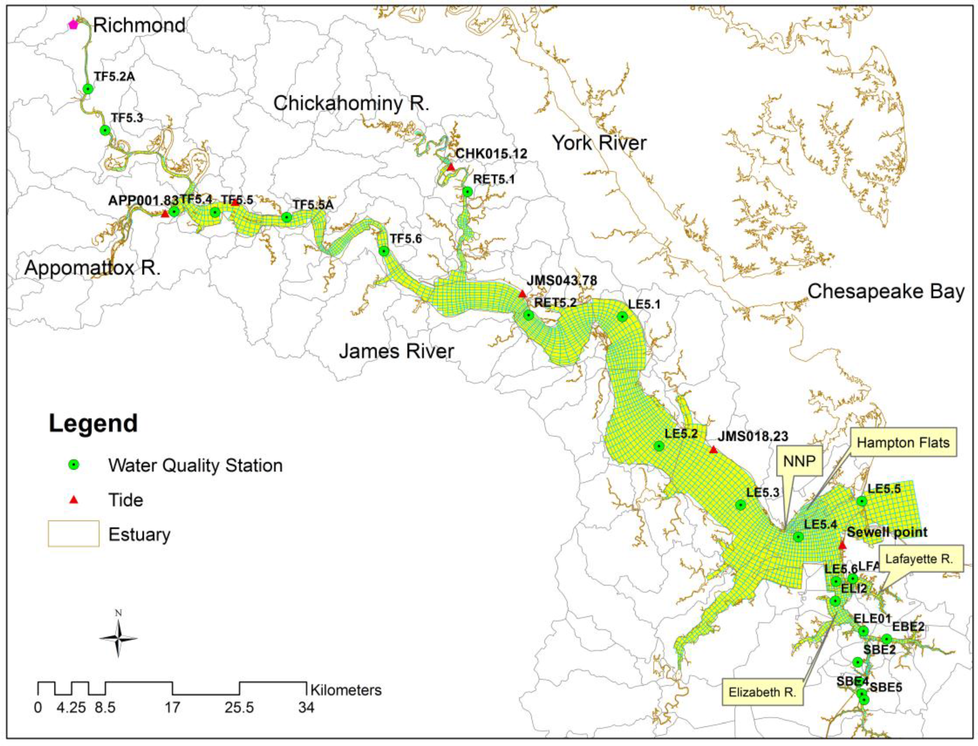
2.1. Study Area

The James River is the southernmost tributary of Chesapeake Bay (Figure 1). It is about 160.0 km long, and the width ranges from 300 m at its upstream and 6 km at the downstream with a mean depth of 3.76 m. The tidal range is about 0.74 m at Sewells Point near the mouth. The mean freshwater discharge is about 226 m³·s⁻¹. The monthly river discharge varies seasonally from 86 m³·s^−l in September to 365 m³·s^−l in March [2]. Salinity in the estuarine part of the James River varies seasonally, which is a common characteristic of estuaries in the mid-latitudes. Near the river mouth, the channel is more than 7 m deep, and salinity typically is around 25 parts per thousand (ppt). The horizontal salinity gradients are usually larger near the upper mesohaline of the river where the freshwater and saltwater converge. The denser, more saline bottom water enters the James River from the Chesapeake Bay and flows upstream, while the less dense surface waters, dominated by freshwater inflow, flow downstream toward the Bay [12,13].

2.2. Model Configuration

The three-dimensional Environmental Fluid Dynamic Code (EFDC) was used for simulations for the James River and its tributaries. The EFDC model is a general hydrodynamic model that solves three-dimensional, time-dependent flows governed by hydrostatic primitive equations [14,15]. The Mellor and Yamada [16] Level 2.5 turbulence closure scheme as modified by Galperin et al. [17] is implemented in the model. The model uses curvilinear, orthogonal horizontal coordinates and sigma vertical coordinates to represent the physical characteristics of a water body. A high-order transport scheme with an anti-numerical diffusion scheme is implemented in the numerical model, which is essential for simulating transport processes accurately in the Chesapeake Bay and its tributaries.

A Cartesian grid model has been applied to the James to study the eddy generated at the mesohaline and polyhaline regions of the lower James [2,18]. The model does not have sufficient resolution for the tidal freshwater region and Elizabeth River to simulate an algal bloom in these regions. A new model grid was developed for the long-term simulation of the dynamic fields. Because the water quality model simulation will span a 23-year period, the efficiency of computation needs consideration. We want to develop a model with sufficient spatial resolution for the simulation of all dynamic features, but maintaining a high efficiency of computation. The model grid cells were designed to follow the main channel of the James River. High resolution was placed on the main stem of the river to obtain the best representation of the topography in this area. The model grid is shown in Figure 1. There are a total of 3066 grid cells in the horizontal and eight layers in the vertical. The bottom bathymetry is interpolated using the NOAA coastal relief model with 90-m resolution (https://www.ngdc.noaa.gov/mgg/coastal/crm.html). For the Elizabeth River, data measured during a survey conducted by the Army Corps (Norfolk District) were used. For small creeks, NOAA charts were used to obtain depths in shallow areas. Eight evenly-spaced sigma layers were applied in the vertical.

The model simulation periods are from 1991 to 2000 and from 2007 to 2013. To allow the model spin-up, the model started from 1990 and 2006, respectively, a full year in advance of each simulation period. Therefore, the impact of the initial conditions can be efficiently removed. Daily river discharges from upstream and lateral watersheds are obtained from the James River watershed model developed by TetraTech, Inc., [19], which includes inflows from 87 sub-watersheds. The three main upstream freshwater discharges are from Richmond, the Appomattox River and the Chickahominy River, respectively. Hourly wind forcing data were obtained from the Norfolk and Richmond International Airports, which are located near the Sewells Point station at the mouth and near the fall line of the James, respectively. The open boundary conditions from 1990 to 2000 (which included hourly time-varying water level, temperature and salinity profiles) were obtained from the 3D model of the Chesapeake Bay Program [20]. Because the Chesapeake Bay Program (CBP) model does not simulate the period from 2006 to 2013, the tide boundary condition for this period used Sewells Point data with corrections of phase and amplitude. The mean differences of phase and amplitude were estimated based on CBP model outputs and measured tidal elevations at Sewells Point. The hourly salinity boundary conditions used for the 2006 to 2013 period are outputs from the large domain Chesapeake Bay model [21,22]. The temperature boundary condition used hourly measurements at Sewells Point at the surface and monthly temperature data measured at CBP Station CB8.1. Differences of surface and bottom temperatures at Station CB8.1 were interpolated in time and applied to the hourly surface temperature data to obtain an estimation of bottom temperature. Because the temperature is highly determined by the air-sea exchange and the open boundary has less impact on the temperature inside the James, this approach yields a good model-data agreement. The radiation boundary conditions are used for the tide, salinity and temperature. Hourly wind forcing, surface pressure, humidity and solar radiation obtained from the hourly meteorological data from Norfolk and Richmond Airports were used for temperature simulations.

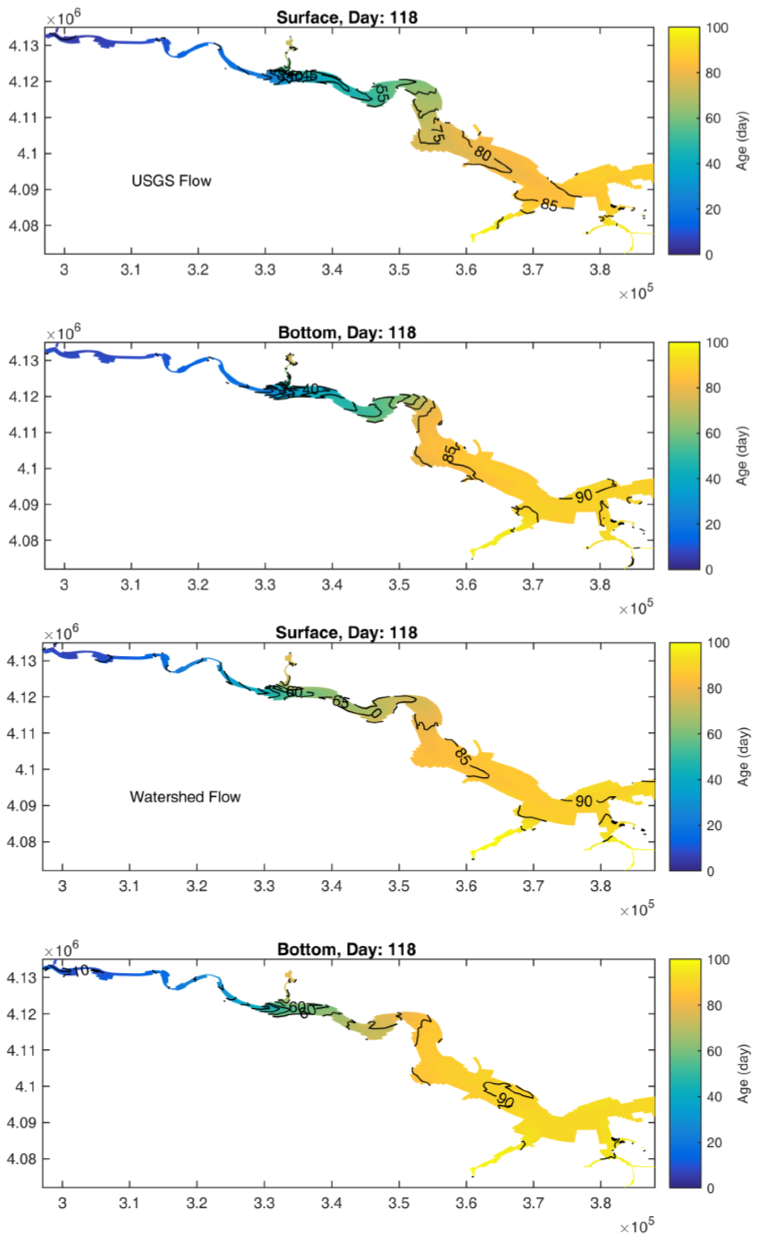
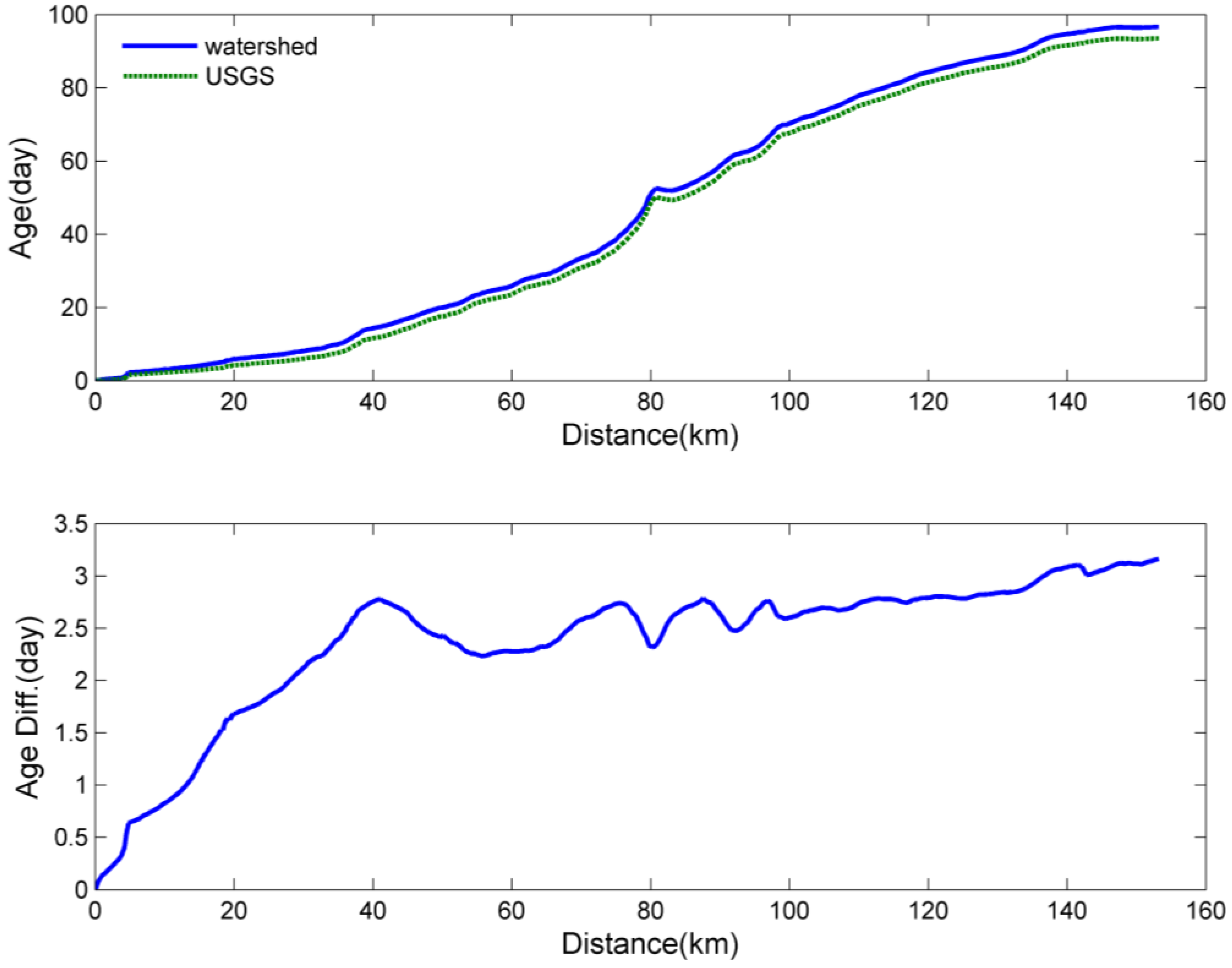
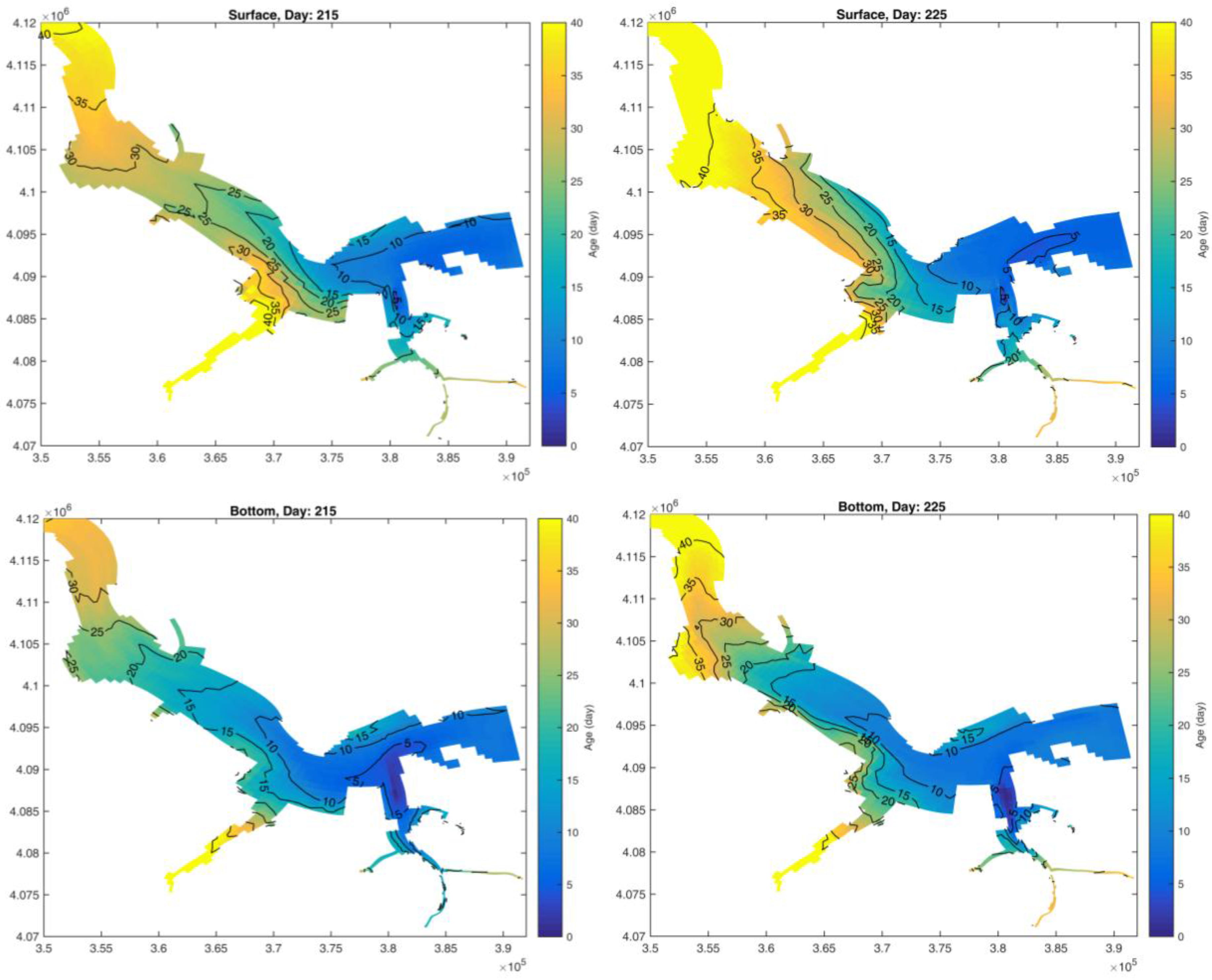
2.3. Age Calculation

Any change of hydrodynamic conditions will result in a change of transport processes, which is more important for transporting both nutrients and phytoplankton [21,22]. Because it is difficult to evaluate the change of dynamic conditions (e.g., change of velocity, surface elevation) and their impact on algae and nutrient transport, we can use the transport timescale to evaluate the impact of dynamics on water quality because it shows a cumulative effect. Transport timescales, such as residence time and renewal time, are the first-order representatives of the dynamic conditions in the estuary, whereas the vertical transport time is directly related to DO exchange [21].

The timescales can be computed using the concept of water age [23]. Freshwater age is the elapsed time since a water parcel leaves the head of a tributary (or any origin), where it has a continual freshwater input. The age at location x is the mean time required for a water parcel to be transported from its discharge location to location x, regardless of its pathway [24]. Delhez et al. [23] provided a way to use a numerical model to compute the water age. Assuming there is only one tracer released to a system without internal sources and sinks, the transport equation for computing the tracer concentration $C(t,\stackrel{\rightharpoonup }{x})$ and the age concentration $\alpha (t,\stackrel{\rightharpoonup }{x})$ can be expressed as [24]:

$$\frac{\partial C(t,\overrightarrow{x})}{\partial t}+\nabla [\overrightarrow{u}C(t,\overrightarrow{x})-K\nabla C(t,\overrightarrow{x})]=0$$

(1)

$$\frac{\partial \alpha (t,\overrightarrow{x})}{\partial t}+\nabla \left[u(t,\overrightarrow{x})\alpha (t,\overrightarrow{x})-K\nabla \alpha (t,\overrightarrow{x})\right]=C(t,\overrightarrow{x})$$

(2)

The mean age can be calculated as follows:

$$a(t,\overrightarrow{x})=\frac{\alpha (t,\overrightarrow{x})}{C(t,\overrightarrow{x})}$$

(3)

where $a(t,\overrightarrow{x})$ is water age, $\nabla =\stackrel{\rightharpoonup }{i}\frac{\partial }{\partial x}+\stackrel{\rightharpoonup }{j}\frac{\partial }{\partial y}+\stackrel{\rightharpoonup }{k}\frac{\partial }{\partial z}$ and K is the diffusivity tensor. To simulate age, the tracer was continuously released at the upstream or at Elizabeth River. The radiation boundary condition was applied at the mouth [18]. Because the upstream of the James River is very narrow, the age has minor variation laterally and vertically. Therefore, the difference of the cross-section average age between its upstream and downstream for a control volume is a good estimate of the local residence time for that control volume.

3. Results

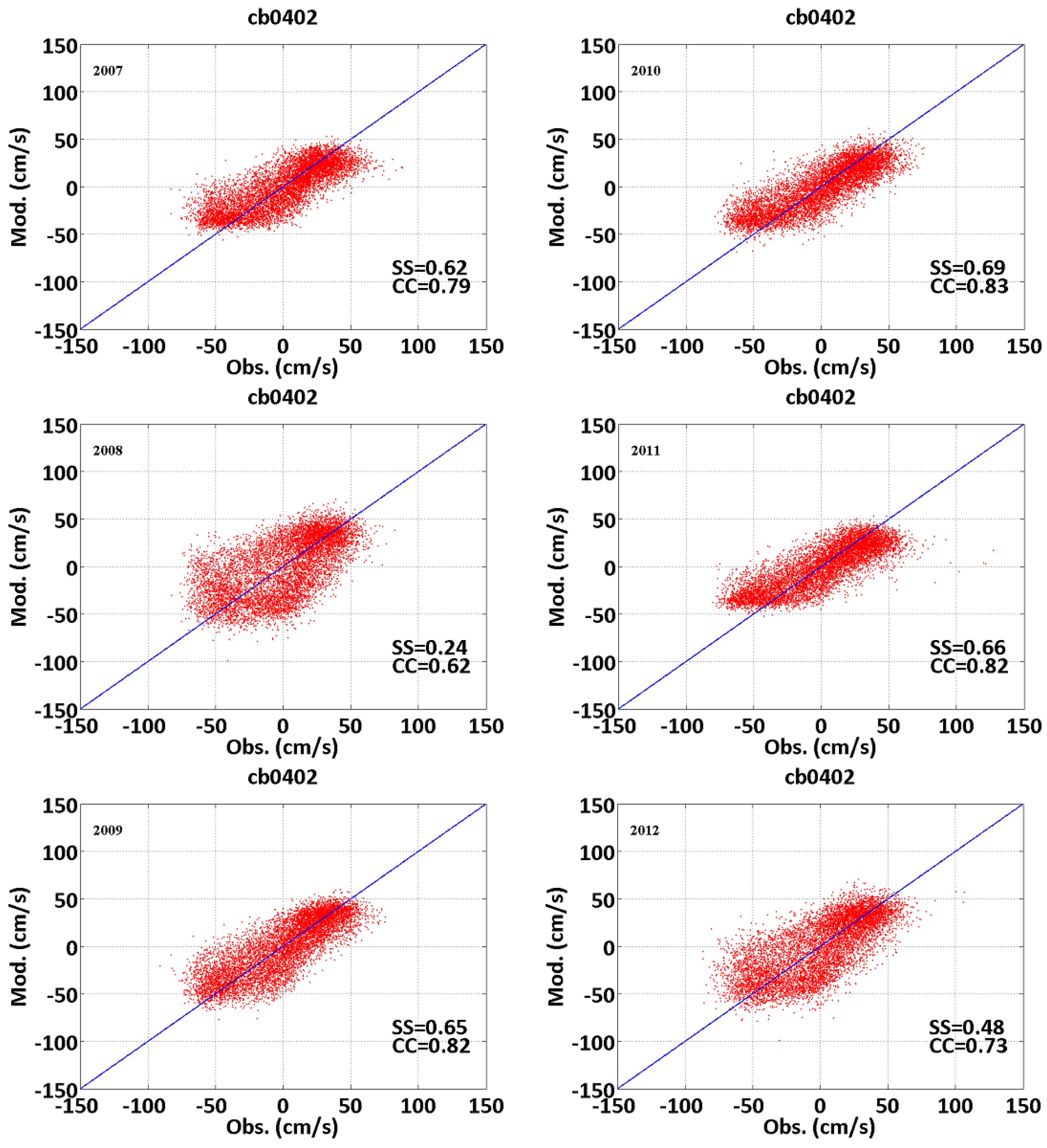
3.1. Tidal Elevation and Current

Model validation for the tide was conducted for the entire simulation period. The surface elevations were compared to the observations at six stations. There is only one NOAA tidal station at Sewells Point. Another five stations are maintained by Virginia Estuarine and Coastal Observing System (VECOS, http://web2.vims.edu/vecos/), which measure water depth using pressure sensors. The bottom roughness height was adjusted to make the tidal propagation correct in the estuary. A constant roughness height of 0.33 cm was used. The statistics of model performance are summarized in the Taylor diagram. The Taylor diagram provides a concise statistical summary of how well patterns match each other in terms of their correlation, their root-mean-square difference and the ratio of their variance [25,26].

Figure 2 shows the model results of tidal elevation. There are three axes shown in the diagram that represent correlation coefficients, the centered root-mean-square difference and standard deviation. All data (both modeled and observed) are normalized by the observed standard deviation at a reference station (APP001.83). The correlation axis shows the correlation between model results and observations. The standard deviation axis indicates the deviation of model results from measurements measured by the standard deviations. The circle of root-mean-square difference shows the root-mean-square difference (RMSD). The value used to normalize the RMSD is 0.3 m.

The modeled surface elevations are within 0.5 RMSD, which is less than 0.15 m. The RMSD is relatively low, and the simulation variations are close to observations based on the measure of the standard deviation, which is close to the reference site as observations. The correlation is larger than 0.86. It can be seen that the tide is well simulated.

In recent years, NOAA has conducted surface current observations in the lower James. The model-simulated currents at a station near EL5-4 are compared to the NOAA observations. Figure 3 shows the scatter plot of observations against the model simulations. The model skill, which is defined as $SS=1-\sum {(A_{model}-A_{obs})}^2/\sum {(A_{obs}-\overline{A_{obs}})}^2$, was used to evaluate the model performance. Performance levels are categorized by the SS value as: >0.65 excellent; 0.65 to 0.5 very good; 0.5 to 0.2 good; <0.2 poor [25]. It can be seen that the model simulations vary each year. Overall, the simulations agree with observations with model correlation ranges from 0.6 to 0.82 and skill between 0.24 and 0.65, indicating that the current simulation is satisfactory. For detailed model results, the readers are referred to the James River Chlorophyll Study Modeling Report [19].

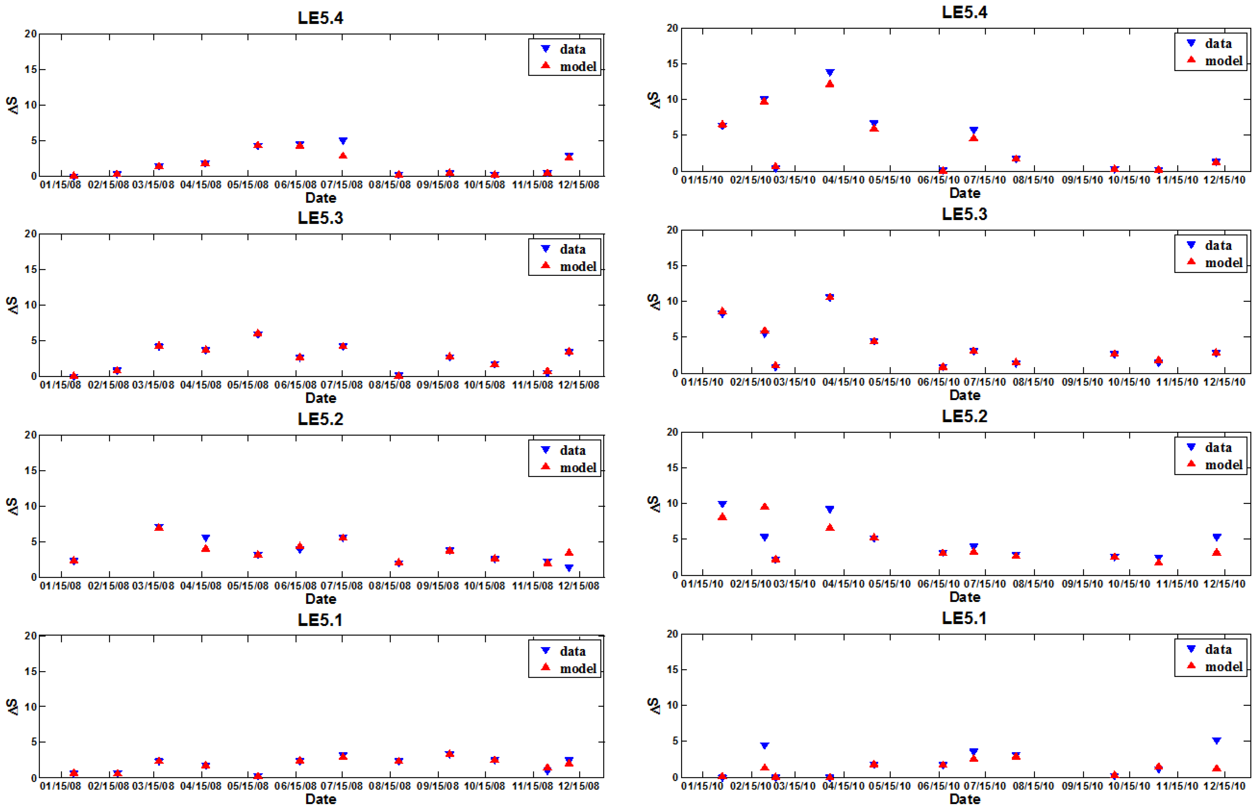
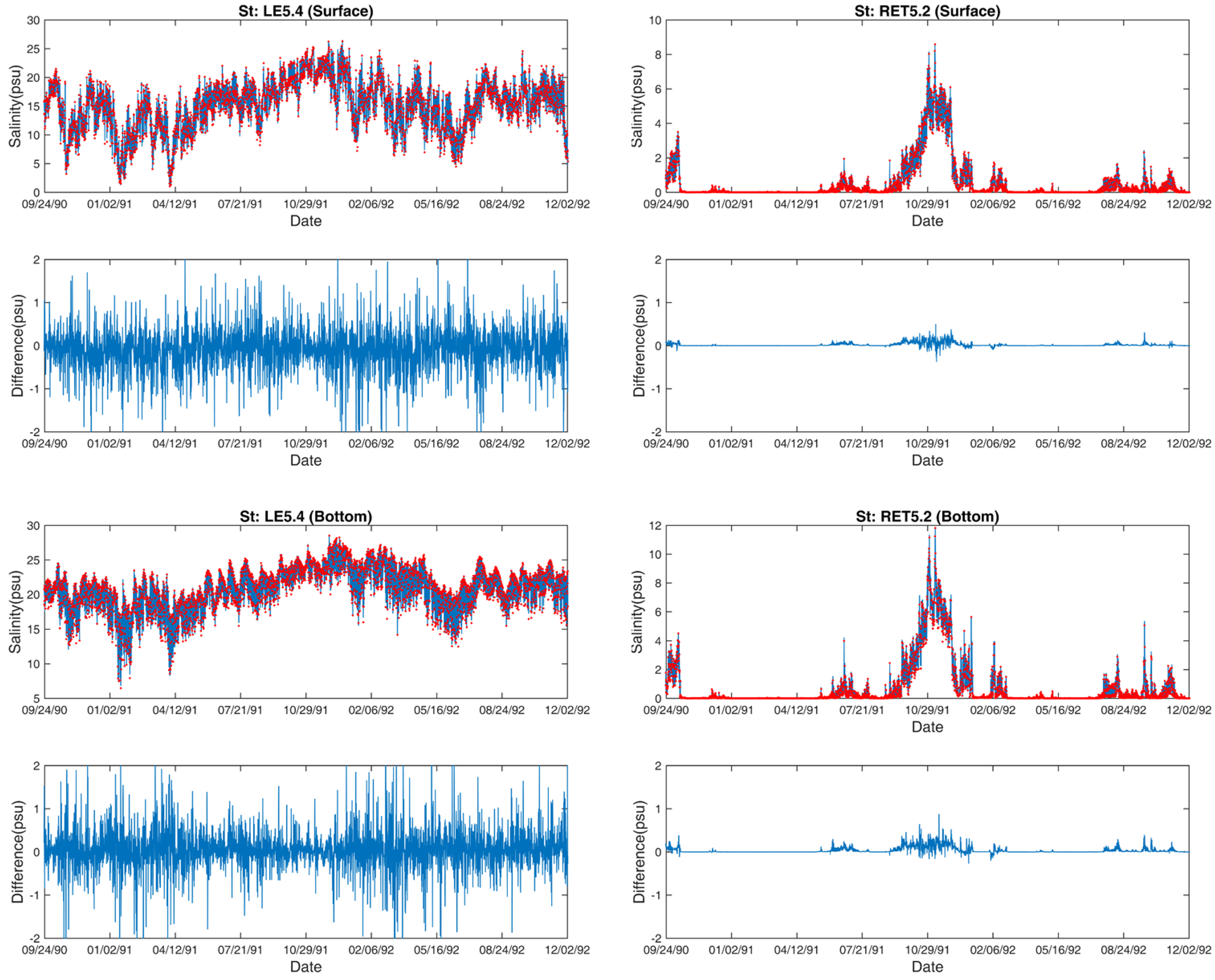
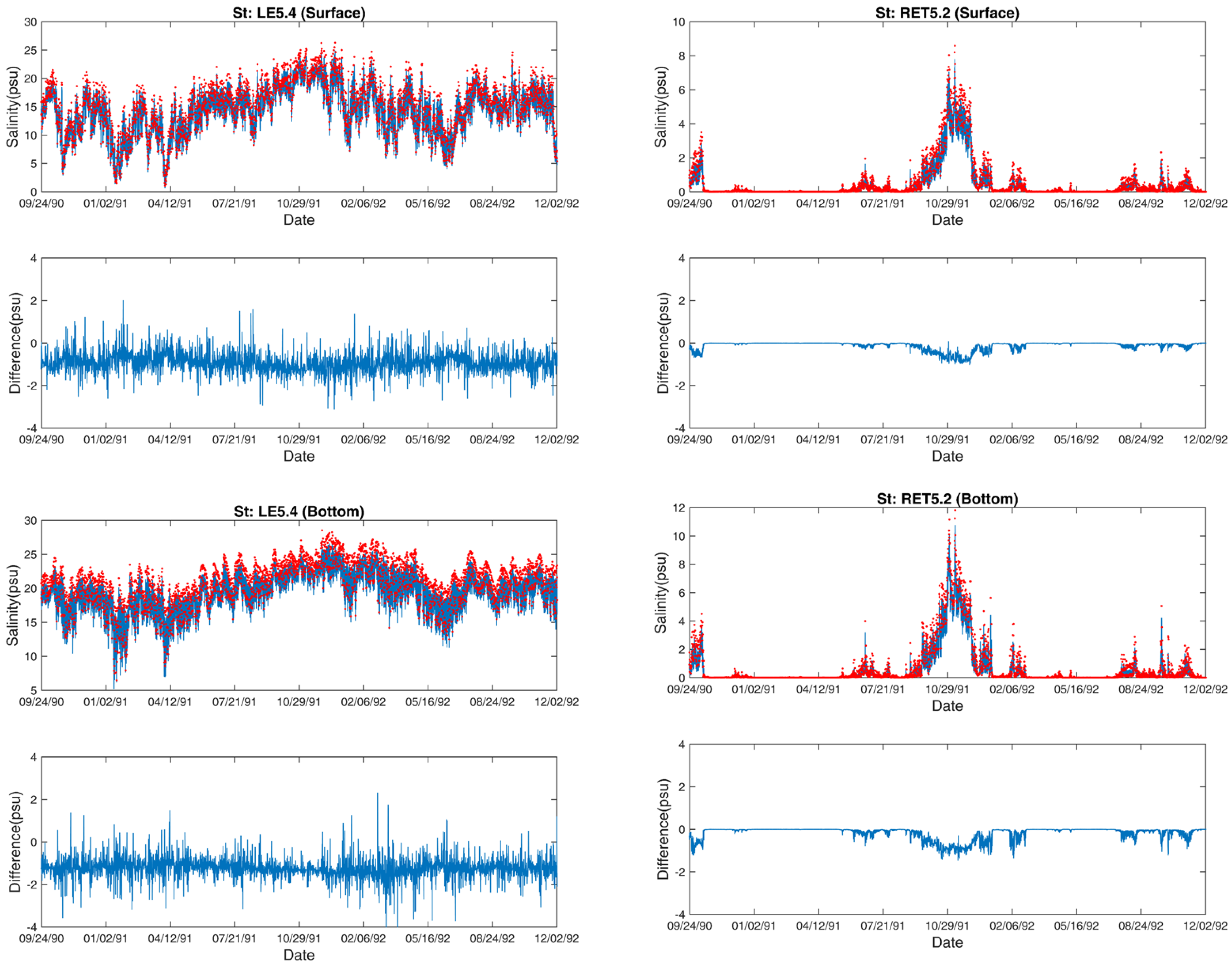
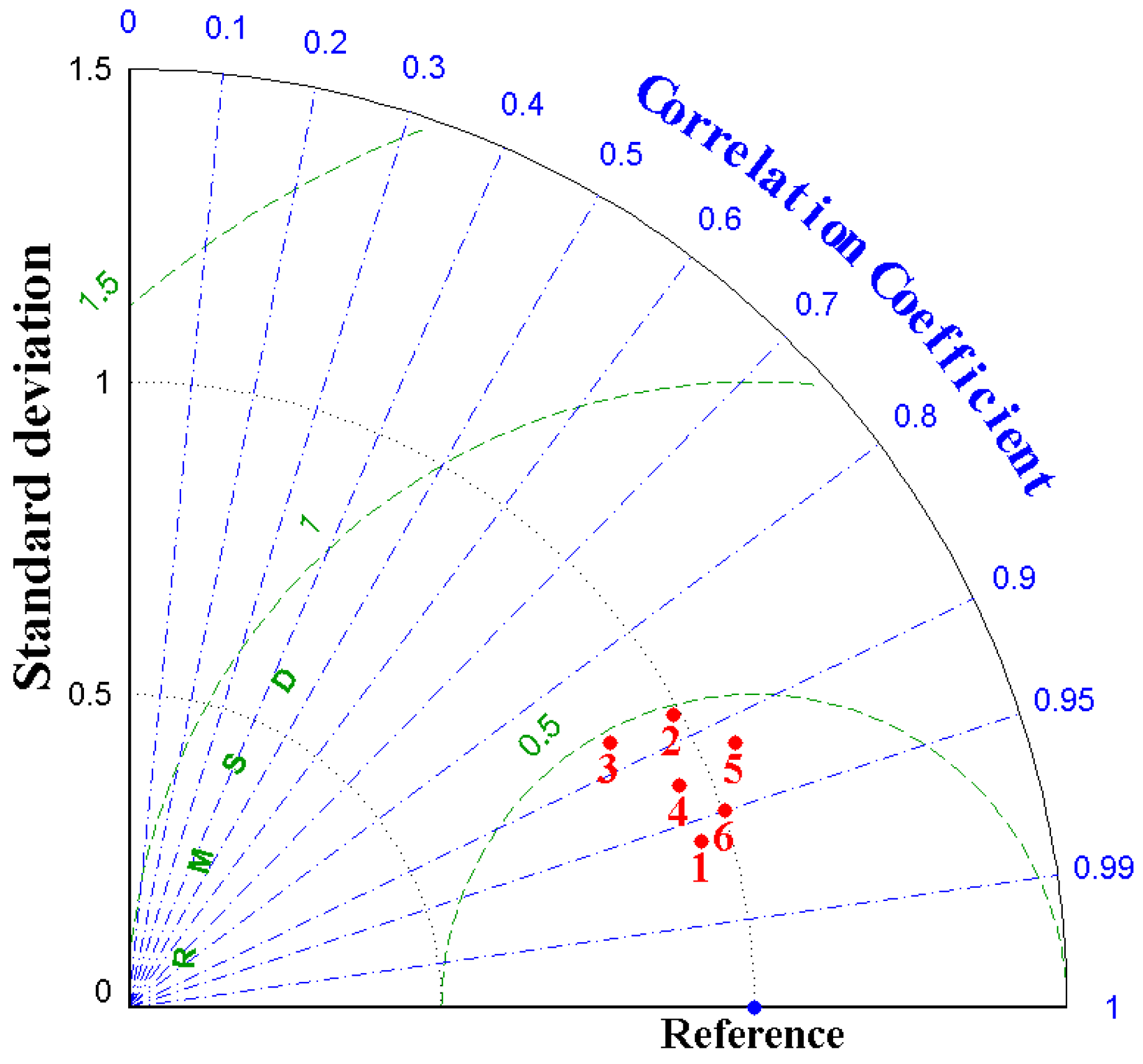
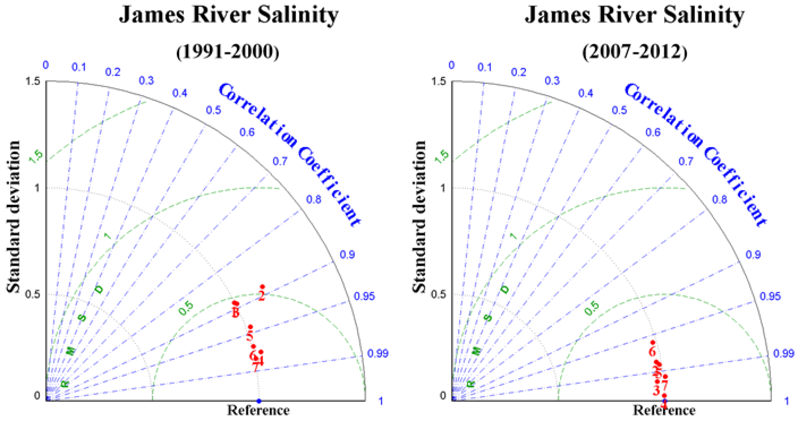
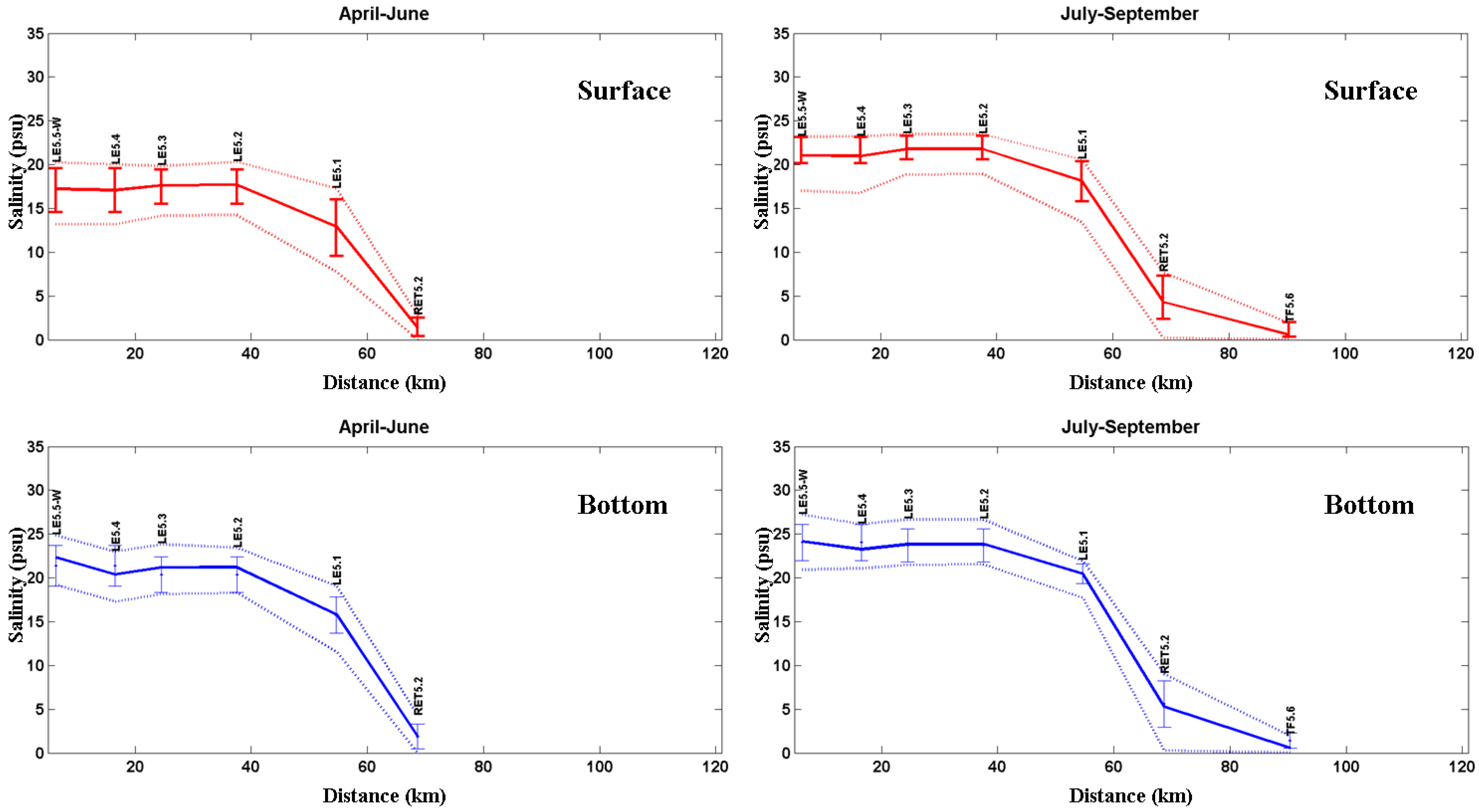
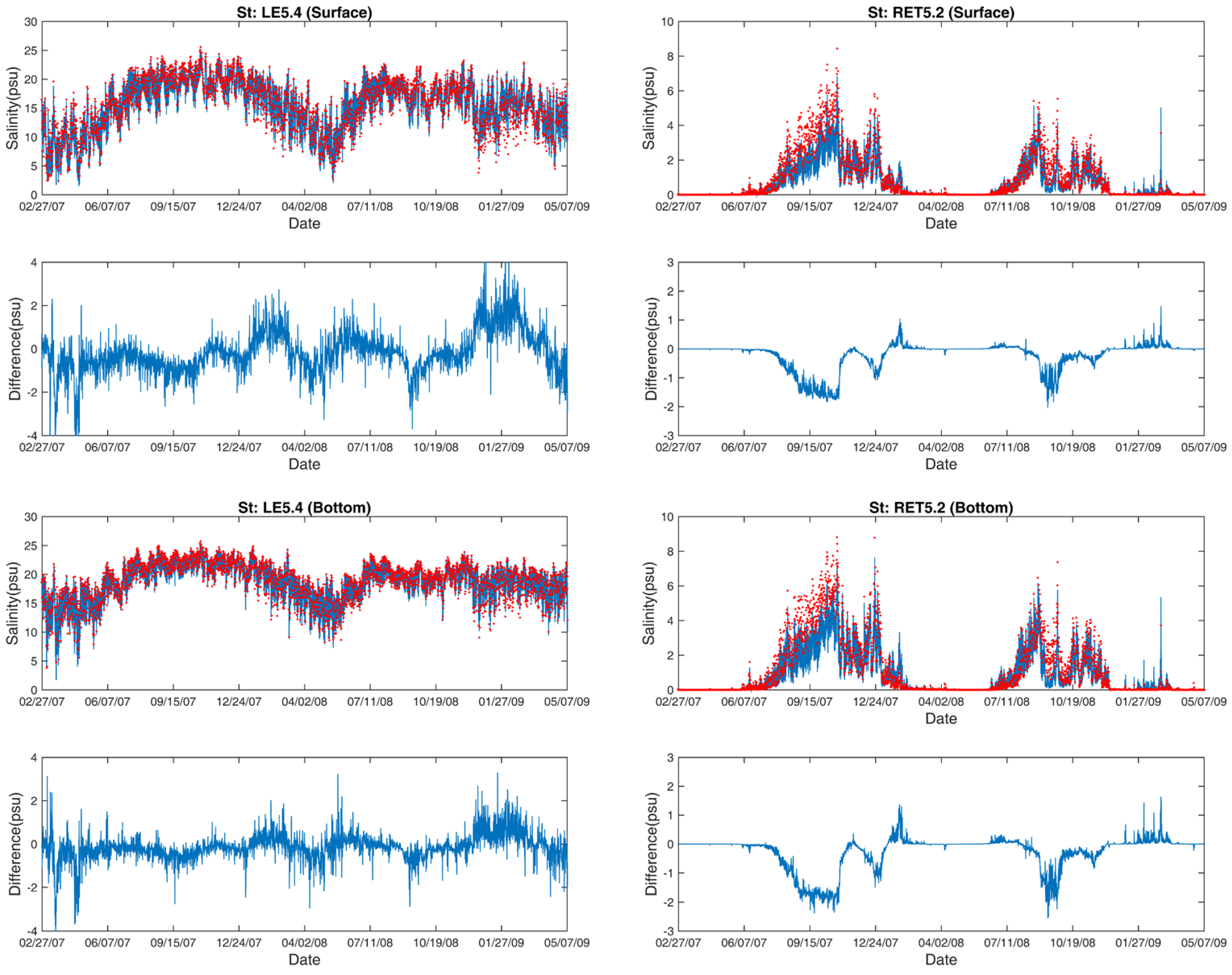
3.2. Salinity

The long-term transport processes are driven by sub-tidal circulation [12]. Correct calibration of salinity is important for accurate simulation of sub-tidal circulation. The calibration of salinity is focused on stratification and salinity intrusion. We used monthly data (measured once a month) to conduct the salinity calibration. The salinity calibration was conducted from 1991 to 2000, and the validation was conducted from 2007 to 2013. Although the data do not have high temporal resolution, these can be used to evaluate a long-term simulation of salinity for seasonal and inter-annual variations. Unlike the model calibration of surface elevation, there are no model parameters to calibrate salinity for the 3D model. The discrepancy of salinity between modeled and observed is mainly caused by the freshwater discharge, boundary condition(s), the wind and bathymetry (which will be discussed in later sections). Both the transport scheme and turbulent scheme used in the model play important roles. EFDC uses a second-order transport scheme with anti-numerical diffusion; it can simulate salinity well in general. The summary of model prediction skill is shown in Figure 4 as a Taylor diagram, in which salinity is compared at seven monitoring stations along the James River (locations are shown in Figure 1). The value used to normalize the root-mean-square difference is 2.39 psu. It can be seen that the model has a high correlation with a low root-mean-square difference at each station. The model performance for the second period is better than that for the first period.

Important characteristics of the salinity simulation are the stratification and salinity intrusion, which are the key parameters that determine gravitation circulations. Examples of salinity stratification (difference between bottom and surface) are shown in Figure 5 for Stations LE5.1, LE5.2, LE5.3 and LE5.4, respectively, for 2008 and 2010. We compared the salinity difference between bottom and surface layers. It can be seen that the model simulated the salinity stratification during this period rather well. The model simulation of salinity intrusion is shown in Figure 6, for surface and bottom salinity. We compared mean, minimum and a maximum of salinity for a three-day window of observations along the James River from the mouth to the salinity intrusion limit and compared it to the observations and their range. It can be seen that the simulation of modeled salinity intrusion agrees well with the observations. The model performance to simulate salinity is satisfactory.

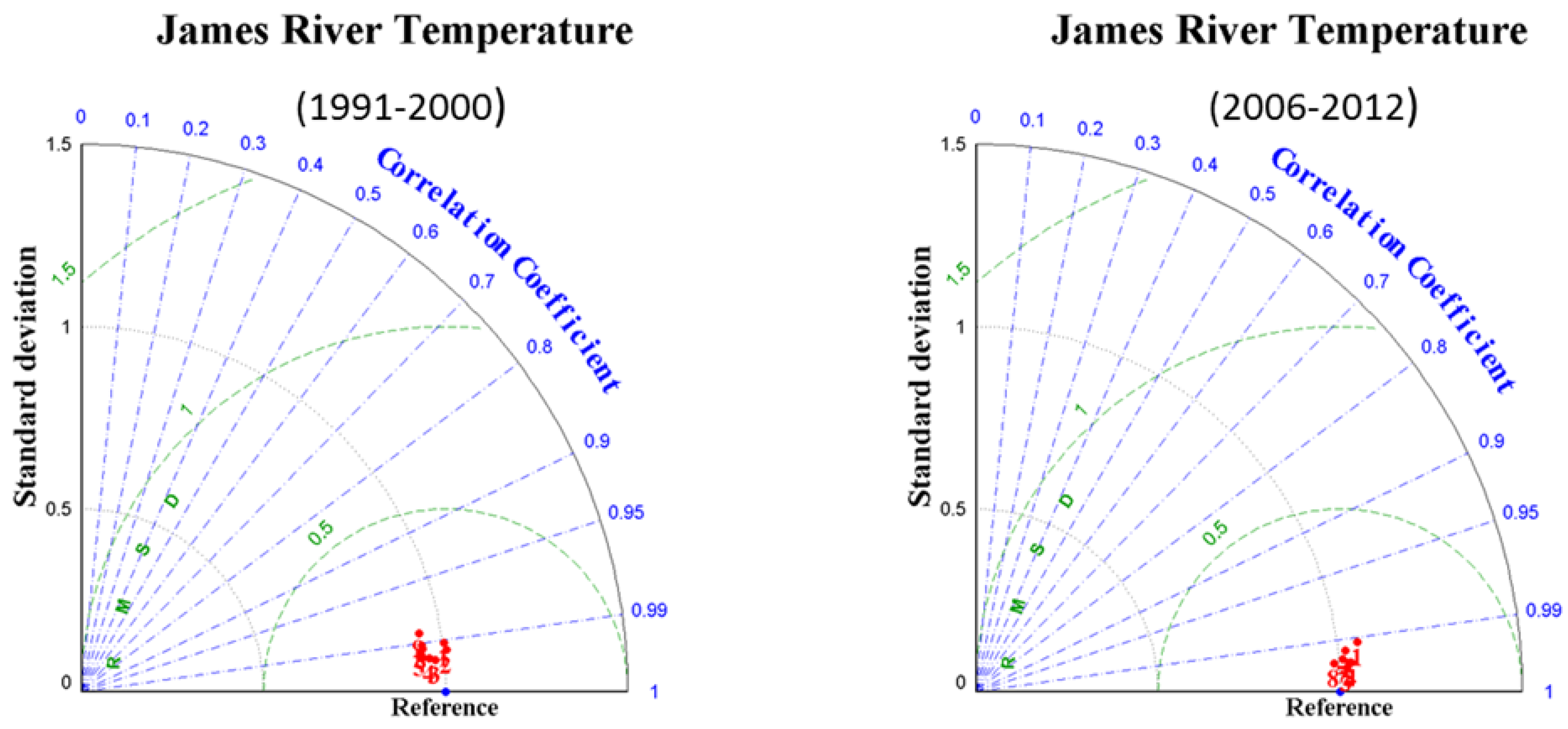
3.3. Temperature

Temperature is a key parameter for the eutrophication model, as all kinetic parameters depend on temperature, which varies from 5 to 30 °C. The observations are monthly (one observation each month at each location). A summary of model prediction skill for temperature simulation is shown in Figure 7 as a Taylor diagram, in which temperature is compared at ten monitoring stations along the James River. It can be seen that the model results include a high correlation at each station with a low root-mean-square difference. There is no difference for all stations statistically for model calibration and validation. The model results are satisfactory.

3.4. Sensitivity Tests

For a three-dimensional model of the EFDC, the logarithmic wall function is used for shear stress. The only model parameter to be calibrated is the bottom roughness height, which determines the model simulation of the tide. However, the external forcing and open boundary conditions are critical for the accurate simulation of salinity, which is important for estuary dynamics and estuarine circulation. A series of model sensitivities is conducted to test the model performance and help understand the impact of external forcing on model performances.

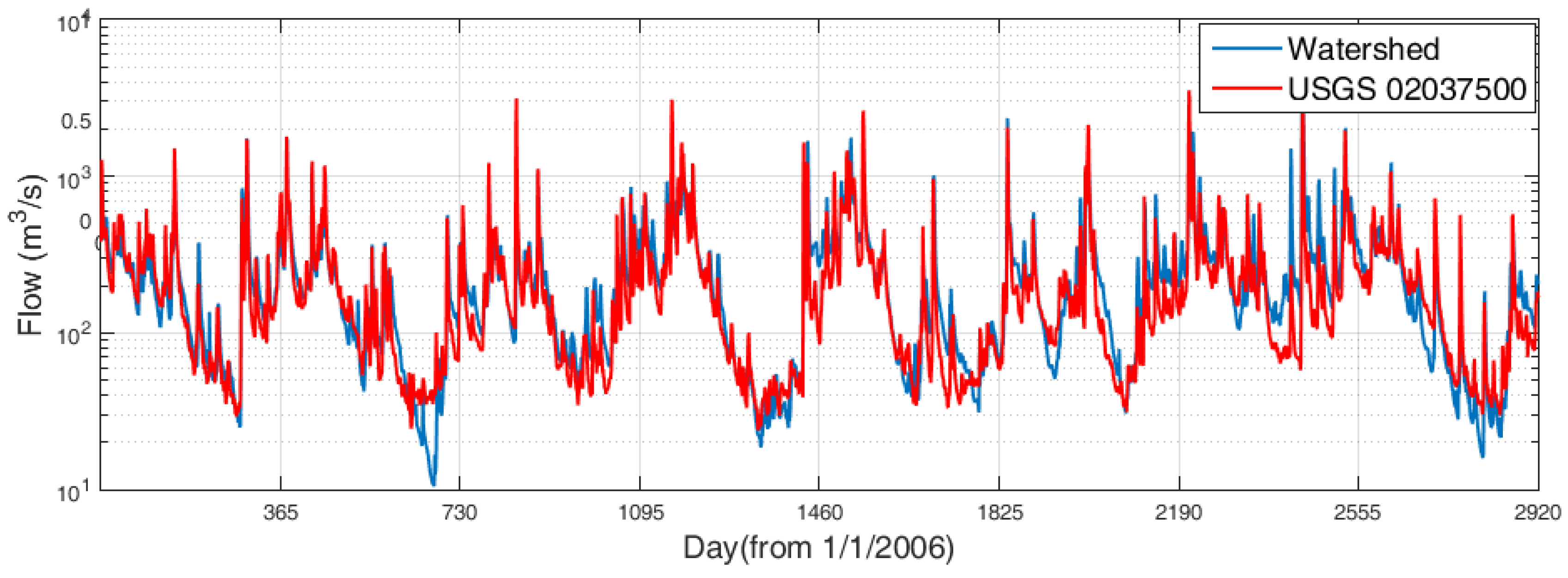
3.4.1. Freshwater Discharge

Estuarine stratification is a competition between barotropic and baroclinic forcings. The large buoyant forcing is from freshwater discharge, which flows out of the estuary on top of the salty, dense water. It can be expected that a change of freshwater discharge can cause a change in salinity. For the current 3D model configuration, we used a watershed model output to drive the model. The model predictive skill is very high, but some discrepancy can be expected, as shown in Figure 8, upstream of Richmond. A sensitivity run was conducted to replace three freshwater discharge input records from locations upstream of Richmond, Appomattox River and Chickahominy River with United States Geological Survey (USGS) flows (USGS02037500, USGS020416500 and USGS02042500). These three stations account for the majority of the flow.

Figure 9 shows the comparison of the salinity difference when using watershed runoff and USGS flow. It can be seen that the model is very sensitive to the flow. The salinity can differ by 2 to 4 psu, which is on the same order as the root-mean-square error of the model calibration. Therefore, some discrepancy during salinity calibration can be expected when using flow from the watershed model.

It is interesting to know if the change of salinity, which is within the accepted error range due to flow or other forcings, will affect the long-term transport or export of nutrients, as the retention of nutrients and eutrophication are highly determined by the residence time [27,28,29]. The transport property of a substance can be quantified by the transport timescales, such as residence time and water age [21,22,23,24]. The age of water is defined as the time elapsed since it leaves the headwaters. The age at each location indicates the time required for the water or conservative substance to travel from the headwaters to a specified location [18]. The age and the residence time are often sufficient to characterize the motions of a conservative substance. We computed the freshwater age along the James River using different flows and compared the results in Figure 10. It can be seen that the transport process is very sensitive to the flow condition. The difference can be about five days for a given period for this example or at a particular day during the high-flow period. The change of flow can affect short-term transport processes. However, the annual mean water age does not change much as shown in Figure 11, especially at the downstream. As the watershed model simulated flow is slightly lower than the USGS flow, even if it is higher during some high-flow periods, the transport slows slightly. However, the results indicate that it will not affect the long-term transport of nutrients in the estuary.

3.4.2. Wind

Wind is a very important forcing to change estuarine circulation. Downstream wind can enhance the estuarine circulation, while upstream wind can increase mixing in the estuary. The wind plays an important role in the modulation of hypoxia in the Chesapeake Bay [30,31]. A sensitivity test to determine the influence of the wind on salinity was conducted. It is unknown if the wind will have a large impact on salinity for this relatively small estuary. We reduced wind forcing by 10%, ran the model from 1990 to 1992 and compared the salinity at Stations LE5.4 and RET5.2, which represents the range of salinity intrusion in the estuary. The sensitivity results are shown in Figure 12. It can be seen that a 10% reduction of wind can change salinity up to 2 psu at Station LE5.4, but causes less than a 0.5-psu change at Station RET5.2. Because the wind-forcing fluctuation has a frequency of three to five days in Chesapeake Bay, the short-term change of the wind on long-term transport appears not to be important for this narrow estuary. We compared water age (not shown here), as well, and found that there is no difference in water age. The results suggest that a 10% error in wind forcing will not affect the long-term transport of nutrients in the James River.

3.4.3. Open Boundary Condition

We used the output of salinity from the large model as the open boundary condition. The influence of the open boundary condition of salinity on the model was evaluated by running the model with a reduction of 5% of the salinity at the open boundary. Comparisons of model results at Stations LE5.4 and RET5.2 are shown in Figure 13. The salinity decreases by about 1.5 psu at Station LE5.4, but only decreases up to 1 psu at Station RET5.2. It can be seen that the salinity simulation is sensitive to the open boundary specification near the mouth. Based on the sensitivity runs, the calibration results are satisfactory, although there are errors in the salinity open boundary condition.

4. Discussion and Summary

The location of an algal bloom not only depends on light and nutrients, but also depends on residence time [28,29]. A correct simulation of transport processes and residence time is critical for the algal bloom. To evaluate the model performance, we computed residence time in the tidal freshwater region and compared the results to the Chl-a observations at Stations TF5.5 and TF5.5A. It can be seen that the peak algal bloom corresponds to the low residence time at that region with a good correlation (R = 0.64, p = 0.001) (Figure 14). Because of the impact of available nutrients and light, it does not match all of the variation as expected. The results indicate that the model simulation transport process is satisfactory and can be used to simulate the HAB.

HABs have occurred almost every year in summer in the mesohaline region of the James, and they are believed to be caused by the HAB bloom initiated in the Lafayette River, a tributary of the Elizabeth River [3]. After a HAB has occurred in the Elizabeth River, the bloom will occur in the James after 10 to 15 days. To verify the transport time for algal transport from the Elizabeth River to the James River, we computed the water age from the Elizabeth River to the James River. The tracer is released from the Elizabeth River; a water age at any location represents the time required for any dissolved materials to be transported from its source to the location. Figure 15 shows the age distribution. It can be seen that it takes about 10 to 15 days to reach the mesohaline region during spring and neap tides. The surface water moves upstream faster during spring tide than during neap tide. The bottom water moves 5–10 days faster upstream than surface water, which is due to the unique front and eddy system near the mouth of the James River [2]. A portion of the ebb flow will turn to the north and flood into the Hampton Flats, where a frontal system is well developed, and surface water will dive to the bottom through this frontal system and be transported upstream along the deep channel near the northern shore. Meanwhile, the flood tide will move surface water upstream [2]. The transport time for water to move from Elizabeth River to the mesohaline region of the James River agrees well with the time delay of the occurrence of the HAB in the James River after the HAB occurred in the Elizabeth River.

In summary, a three-dimensional hydrodynamic model has been developed for the James River. The Environmental Fluid Dynamics Computer Code (EFDC) is used for developing the James River hydrodynamic model. The model was calibrated for surface elevation over the period from 2006 to 2008, for current over the period from 2007 to 2012 and for salinity and temperature from 1991 to 2000. Furthermore, it is validated from 2007 to 2013 for salinity and temperature. The model validation results indicate that the model is robust; it adequately simulates the hydrodynamics and temperature; and it is suitable for the water quality model development for the James River.

References

- Bukaveckas, P.; Barry, L.E.; Beckwith, M.J.; David, V.; Lederer, B. Factors determining the location of the chlorophyll maximum and the fate of algal production within the tidal freshwater James River. Estuar. Coasts 2011, 34, 569–582. [Google Scholar] [CrossRef]
- Shen, J.; Boon, J.; Kuo, A.Y. A numerical study of a tidal intrusion front and its impact on larval dispersion in the James River estuary, Virginia. Estuaries 1999, 22, 681–692. [Google Scholar] [CrossRef]
- Morse, R.E.; Shen, J.; Blanco-Garcia, J.L.; Hunley, W.S.; Fentress, S.; Wiggins, M.; Mulholland, M.R. Environmental and physical controls on the formation and transport of blooms of the dinoflagellate Cochlodinium polykrikoides Margalef in the lower Chesapeake bay and its tributaries. Estuar. Coasts 2011, 34, 1006–1025. [Google Scholar] [CrossRef]
- Sheng, Y.P. A Three-Dimensional Mathematical Model of Coastal, Estuarine and Lake Currents Using Boundary-Fitted Grid; Technical Report No. 585; Aeronautical Research Associates of Princeton: Princeton, NJ, USA, 1986. [Google Scholar]
- Cheng, R.T.; Casulli, V.; Gartner, J.W. Tidal residual intertidal mudflat (TRIM) model and its applications to San Francisco Bay, California. Estuar. Coast. Shelf Sci. 1993, 36, 235–280. [Google Scholar] [CrossRef]
- Cerco, C.F.; Cole, T. Three-Dimensional Eutrophication Model of Chesapeake Bay, Volume I: Main Report; EL-94.4; U.S. Army Corps of Engineers Waterway Experiment Station: Vicksburg, MS, USA, 1994. [Google Scholar]
- Wool, T.A.; Ambrose, R.B.; Martin, J.L.; Comer, E.A. Water Quality Analysis Simulation Program (WASP); version 6.0; Draft User’s Manual; United States Environmental Protection Agency: Atlanta, GA, USA, 2001.
- Wan, Y.; Ji, Z.; Shen, J.; Hu, G.; Sun, D. Three dimensional modeling of a shallow subtropical estuary. Mar. Environ. Res. 2012, 82, 76–86. [Google Scholar] [CrossRef] [PubMed]
- Testa, J.M.; Kemp, W.M.; Boynton, W.R.; Hagy, J.D. Longterm changes in water quality and productivity in the Patuxent River estuary: 1985 to 2003. Estuar. Coasts 2008, 31, 1021–1037. [Google Scholar] [CrossRef]
- Chen, C.; Liu, H.; Beardsley, R.C. An unstructured, finite-volume, three-dimensional, primitive equation ocean model: Application to coastal ocean and estuaries. J. Atmos. Ocean. Technol. 2003, 20, 159–186. [Google Scholar] [CrossRef]
- Cerco, C.F.; Kim, S.; Nole, M.R. The 2010 Chesapeake Bay Eutrophication Model; A Report to the US Environmental Protection Agency Chesapeake Bay Program and to the US Army Engineer Baltimore District; US Army Engineer Research and Development Center: Vicksburg, MS, USA, 2010. [Google Scholar]
- Pritchard, D.W. The dynamic structure of a coastal plain estuary. J. Mar. Res. 1956, 15, 33–42. [Google Scholar]
- Kuo, A.Y.; Neilson, B.J. Hypoxia and salinity in Virginia estuaries. Estuaries 1987, 10, 277. [Google Scholar] [CrossRef]
- Hamrick, J.M. A Three-Dimensional Environmental Fluid Dynamics Code: Theoretical and Computational Aspects; VIMS SRAMSOE #317; College of William and Mary, Virginia Institute of Marine Science: Gloucester Point, VA, USA, 1992; p. 63. [Google Scholar]
- Park, K.; Kuo, A.Y.; Shen, J.; Hamrick, J.M. A Three-Dimensional Hydrodynamic Eutrophication Model (HEM-3D): Description of Water Quality and Sediment Process Submodels; Special Report in Applied Marine Science and Ocean Engineering No. 327; Virginia Institute of Marine Science: Gloucester Point, VA, USA, 1995; p. 102. [Google Scholar]
- Mellor, G.L.; Yamada, T. Development of a turbulence closure model for geophysical fluid problems. Rev. Geophys. Space Phys. 1982, 20, 851–875. [Google Scholar] [CrossRef]
- Galperin, B.; Kantha, L.H.; Hassis, S.; Rosati, A. A quasi-equilibrium turbulent energy model for geophysical flows. J. Atmos. Sci. 1988, 45, 55–62. [Google Scholar] [CrossRef]
- Shen, J; Lin, J. Modeling study of the influences of tide and stratification on age of water in the tidal James River. Estuar. Coast. Shelf Sci. 2006, 68, 101–112. [Google Scholar] [CrossRef]
- Chesapeake Environmental Communications (CEC). Modeling Support for the James River Chlorophyll Study: Modeling Report, prepared by CRC, HDR, Tetra Tech, and Virginia Institute of Marine Science for Virginia Department of Environmental Quality: Richmond, VA, USA, February 29, 2015.
- Cerco, C.; Noel, M. The 2002 Chesapeake Bay Eutrophication Model; EPA 903-R-04-004; US Army Engineer Research and Development Center: Vicksburg, MS, USA, 2004. [Google Scholar]
- Du, J.; Shen, J. Decoupling the influence of biological and physical processes on the dissolved oxygen in the Chesapeake Bay. J. Geophys. Res. Oceans 2015, 120, 78–93. [Google Scholar] [CrossRef]
- Hong, B.; Shen, J. Linking dynamics of transport timescale and variation of hypoxia in the Chesapeake Bay. J. Geophys. Res. 2013, 118, 6017–6029. [Google Scholar] [CrossRef]
- Delhez, E.J.M.; Campin, J.M.; Hirst, A.C.; Deleersnijder, E. Toward a general theory of the age in ocean modeling. Ocean Model. 1999, 1, 17–27. [Google Scholar] [CrossRef]
- Deleersnijder, E.; Campin, J.M.; Delhez, E.J.M. The concept of age in marine modeling: I. Theory and preliminary model results. J. Mar. Syst. 2001, 28, 229–267. [Google Scholar] [CrossRef]
- Wilmott, C.J. On the validation of models. Phys. Geogr. 1981, 2, 184–194. [Google Scholar]
- Taylor, K.E. Summarizing multiple aspects of model performance in a single diagram. J. Geophys. Res. 2001, 106, 7183–7192. [Google Scholar] [CrossRef]
- Nixon, S.W.; Ammerman, J.W.; Atkinson, L.P.; Berounsky, V.M.; Billen, G.; Boicourt, W.C.; Boynton, W.R.; Church, T.M.; Ditoro, D.M.; Elmgren, R.; et al. The fate of nitrogen and phosphorus at the land-sea margin of the North Atlantic Ocean. Biogeochemistry 1996, 35, 141–180. [Google Scholar] [CrossRef]
- Lucas, L.V.; Thompson, J.K.; Brown, L.R. Why are diverse relationships observed between phytoplankton biomass and transport time. Limnol. Oceanogr. 2009, 54, 381–390. [Google Scholar] [CrossRef]
- Peierls, B.L.; Hall, N.S.; Paerl, H.W. Non-monotonic responses of phytoplankton biomass accumulation to hydrologic variability: A comparison of two coastal plain North Carolina estuaries. Estuar. Coasts 2012, 35, 1376–1392. [Google Scholar] [CrossRef]
- Scully, M.E. Wind modulation of dissolved oxygen in Chesapeake Bay. Estuar. Coasts 2010, 33, 1164–1175. [Google Scholar] [CrossRef]
- Shen, J.; Hong, B.; Kuo, A.Y. Using timescales to interpret dissolved oxygen distributions in the bottom waters of Chesapeake Bay. Limnol. Oceanogr. 2013, 28, 2237–2248. [Google Scholar] [CrossRef]
© 2016 by the authors; licensee MDPI, Basel, Switzerland. This article is an open access article distributed under the terms and conditions of the Creative Commons Attribution license ( http://creativecommons.org/licenses/by/4.0/).
Share and Cite
Shen, J.; Wang, Y.; Sisson, M. Development of the Hydrodynamic Model for Long-Term Simulation of Water Quality Processes of the Tidal James River, Virginia. J. Mar. Sci. Eng. 2016, 4, 82. https://doi.org/10.3390/jmse4040082
Shen J, Wang Y, Sisson M. Development of the Hydrodynamic Model for Long-Term Simulation of Water Quality Processes of the Tidal James River, Virginia. Journal of Marine Science and Engineering. 2016; 4(4):82. https://doi.org/10.3390/jmse4040082
Chicago/Turabian StyleShen, Jian, Ya Wang, and Mac Sisson. 2016. "Development of the Hydrodynamic Model for Long-Term Simulation of Water Quality Processes of the Tidal James River, Virginia" Journal of Marine Science and Engineering 4, no. 4: 82. https://doi.org/10.3390/jmse4040082