1. Introduction
The sound field measured at a receiver in the ocean contains information about the physical characteristics of the ocean waveguide through which the sound has propagated. This basic fact is evident from the theories of sound propagation in the ocean, and has been known since the time of the early works of research pioneers in ocean acoustics [
1,
2]. However, development of formal methods to invert acoustic field data for estimates of waveguide characteristics, such as geoacoustic properties of the ocean bottom was limited by the lack of sufficient computing power to implement computationally-intensive inversion techniques. Instead, early applications of inversions were confined to simple procedures such as making subjective changes of specific ocean bottom model parameters in attempts to improve predictions of propagation loss or bottom loss data [
3,
4,
5].
Our ability to implement inversion algorithms has improved dramatically over the past three decades with significant advances in computing technology and numerical sound propagation models [
6,
7,
8]. Since around 1990, there has been considerable research efforts to develop experimental and theoretical inversion techniques to estimate characteristics of the ocean bottom from the acoustic measurements. Inversion methods in ocean acoustics can be described as model-based techniques that take advantage of the relationship between the acoustic field and the waveguide model parameters through the wave equation. Generally, the inversions are carried out by comparing measured data with calculated replicas of the acoustic field or an appropriate quantity derived from the field, and there are many reports in the recent literature about inversion techniques and applications with experimental data. Examples include matched field inversion of pressure field data using optimization algorithms, such as simulated annealing [
9,
10], genetic algorithms [
11], and advanced Bayesian approaches [
12,
13] that can be applied to pressure data or other quantities derived from the acoustic field, such as ocean bottom reflection coefficients or modal group velocities. Although the relationship between the acoustic field and the waveguide parameters is inherently nonlinear, linearized relations can be developed for some field quantities, such as mode wavenumbers. This approach was developed by Rajan et al. [
14]. These inversion methods have introduced powerful new techniques in acoustical oceanography for extracting information about the ocean from acoustic data.
This paper focuses on geoacoustic inversion, and describes an application of Bayesian inference to invert ocean bottom reflection coefficient data from experiments with broadband sound sources at deep water sites in the Pacific Ocean. The motivation for the experiments was to determine the variation of compressional and shear speeds in upper oceanic crust as the age of the basalt increased westward, away from the ocean spreading center. The experiments were carried out from 1986 to 1992, and initial results for the inversion of sound speed using an optimization approach with simulated annealing were reported in 1994 [
15]. In this paper, the inversion is re-examined using Bayesian inference.
The formalism of Bayesian inversion is reviewed first in
Section 2 to establish an understanding of the approach for estimation of geoacoustic model parameters that is in widespread use in acoustical oceanography. The method is then applied to invert the ocean bottom reflection coefficient versus angle data from the experiments. The data were obtained using an unconventional experimental technique that was designed to determine both the compressional and shear wave speeds in the uppermost portion of oceanic crust. The technique is based on measurements of the ocean bottom reflection loss versus grazing angle, using small explosive charges as sound sources. This approach has been widely used in acoustical oceanography to measure acoustic propagation loss and to characterize the ocean bottom in terms of geoacoustic profiles. The experimental technique and the method for deriving the reflection coefficient data are described in
Section 3. The inversion results for the geoacoustic model parameters for the different sites presented in
Section 3.4 indicate that crustal ageing is active over the experimental track where the age increased from 40 to 70 million years (m.y.). The results of the inversions are discussed in the context of models of crustal ageing processes in
Section 4.
2. Bayesian Geoacoustic Inversion
The interaction of sound with the ocean bottom is introduced into calculations of the acoustic field using geoacoustic models that consist of layered structures of sound speed, attenuation, and density of the ocean bottom materials. Generally, the layers are assumed to be fluids, but depending upon the ocean bottom environment, the model can also include shear wave parameters in the layers. Inversion methods are designed to estimate values of the geoacoustic model parameters, and provide statistically valid measures of the uncertainty of the estimates.
The Bayesian approach for estimating geoacoustic model parameters is in widespread use in acoustical oceanography, and has been applied to pressure field data and data representing other observable quantities derived from the acoustic field. The Bayesian solution to the inverse problem is presented in terms of probabilities of all models within an allowed set of possible models that are constrained within pre-set bounds for the model parameter values. Models with higher probabilities are more likely to be realistic representations of the real ocean environment. An outline of the formalism of Bayesian inference is described below.
The method is based upon Bayes relation between the experimental data,
d, and the geoacoustic model parameters,
m. Both the data and the model parameters are assumed to be random variables. Bayes relation is expressed in terms of conditional probabilities:
In this equation
is the conditional probability density function (PDF) of the model given the experimental data and
is the PDF of the data for the selected model parameterization. If
d are the observed data,
can be taken as equal to one.
is the conditional PDF of the data given a model
m, and
is the PDF of the model
m. Since the models are assumed to be random variables,
is interpreted as the distribution of models based on prior knowledge of the ocean bottom environment. In most cases, a uniform distribution of models is assumed, within selected bounds of possible parameter values. Equation (1) states that Bayesian inference involves an interaction that combines the information about the model contained in the data,
, and the prior knowledge about the model,
. In an inversion, new information about the model is obtained from the data by performing tests of how well the candidate models predict the observed data in calculations of replicas of the data. The number of possible models includes all possible combinations of the different model parameters that are allowed in the geoacoustic model. Even for a relatively simple single-layer model as in
Figure 1, it is evident that the number of possible models that must be tested is very large.
To proceed further it is necessary to develop an expression for
. In Bayesian inference,
is interpreted as a likelihood function:
where
expresses the mismatch between the data and predictions of the data based on the model. From Equation (1),
can be expressed in terms of a generalized mismatch that combines information about the model from both the data and the prior knowledge:
In Bayesian inference,
represents the complete solution of the inverse problem, and is called the
a posteriori probability density or the PPD. For geoacoustic inversion, the PPD expresses the probability of a given model being a likely representation of the real ocean bottom. Models with higher probability are expected to be more likely representations of the real environment. However, the PPD is a multi-dimensional quantity, the dimensions of which depend upon the number of model parameters that are estimated in the inversion. The challenge in Bayesian inference is to interpret the multi-dimensional PPD in terms of model parameter estimates and uncertainties. This requires numerical computation of properties of the PPD such as the maximum a posteriori (MAP) model estimate, the mean model estimate, the model covariance matrix and marginal probability distributions. These are defined as:
respectively. In Equation (7), the one-dimensional marginal probability distribution, δ is the Dirac delta function. Higher-dimensional marginal probability distributions are defined similarly.
To implement Bayesian inference, it is necessary to specify the relation between the observed data and the set of environmental model parameters to define the mismatch function
in Equation (2). The relation can be interpreted in terms of the mismatch between the measurement and a prediction of the measurement
q based on the model:
The mismatch n can be interpreted as noise arising from uncertainty in the experimental data itself, theory errors owing to differences between the environmental model and the real Earth or differences caused by an inaccurate physical theory of sound propagation in the ocean. The statistical distribution of n is generally not known, and it is convenient to assume a Gaussian distribution.
For assumed Gaussian errors, the misfit function,
, is given by:
where † denotes the Hermitian transpose and
Cd is the data error covariance matrix. In many applications, the covariance matrix is assumed to be diagonal,
, where σ is the standard deviation of uncorrelated errors assumed to be the same at each receiver and
I is the identity matrix. For this condition, the likelihood function (Equation (2)) becomes:
where
N is the number of receivers at which data are recorded.
This brief outline summarizes the basic assumptions and theory of Bayesian inference. More detail of the implementation of the approach for one of the most widely used approaches, matched field inversion, can be found in the series of papers by Dosso and co-authors [
12,
16] and in Jiang and Chapman [
17]. In the next section, an application of Bayesian inversion of ocean bottom reflection loss data is presented.
3. Inversion of Geoacoustic Properties of Young Oceanic Crust
This section describes the data acquisition and signal processing techniques that were used to obtain the reflection coefficient versus angle data at the thin-sediment upper crust sites. A brief background of evolution of young oceanic crust is described first to provide the setting for the experiments. The acoustic reflectivity at thin-sediment upper crust sites is described next to introduce the geoacoustic model that was used to describe the ocean bottom in the inversions. The experimental technique is presented in
Section 3.3 to describe the data acquisition process and signal processing that were used to obtain the reflection coefficient data at each experimental site. The last section presents the results of the Bayesian inversion.
3.1. Evolution of Young Oceanic Crust
In large areas of the Pacific Ocean, the sediment deposits are very thin and oceanic crustal basalt is close to the sea floor. Oceanic crust is created at mid-ocean spreading ridges where basalt material is erupted at the sea floor by magmatic processes. The young, newly-formed basalt is highly fractured with cracks, but the rock structure changes with time as the young crust moves away from the spreading centers and ages over geological time. Early geophysical studies of oceanic crust focused on measurements of sound speed in basalt. However, measurements done in laboratories indicated high values (~5.5 km/s) that were inconsistent with sound speeds as low as ~3.3 km/s inferred from seismic refraction profiles at sea. To resolve the disparity in the different results, Houtz and Ewing proposed that the sound speed in crustal basalt changed as the rock aged over time [
18]. They suggested a simple model for oceanic crust that featured an uppermost surface layer, Layer 2A, in which the sound speed changed as the rock structure changed during the ageing process.
The increase in sound speed is generally attributed to alteration of the physical properties of the crustal basalt associated with hydrothermal circulation at low temperatures within the ridge crest and flanks [
19,
20]. In this model, minerals are precipitated in the cracks and voids of the young basalt as ocean water circulates in the rock structure over time. The hydrothermal alteration and deposition process is temperature dependent, and is strongly affected by the overlying sediment cover which can insulate the crust from the ocean water. This increases the temperature in the crust and the rate of alteration accelerates [
20,
21]. The rate of ageing is not uniform worldwide, but is dependent upon the ridge flank environment at each site.
Both the compressional and shear wave speeds in the basalt are expected to increase as the cracks and voids are filled in the ageing process. Since the initial work of Houtz and Ewing, conventional seismic refraction and reflection surveys with towed streamers and ocean bottom seismometers have been carried out at different ridge sites [
22,
23,
24]. The experiments provided results indicating low values in the range 2.2–2.5 km/s for the compressional wave speed in young basalt. However, there is relatively little information about the shear wave speed and its variation with crustal age.
This paper introduces new inversion results from an experimental technique that provided estimates of both the compressional and shear wave speeds in the uppermost portion of upper crust basalt. The reflection characteristics from an elastic solid system of ocean bottom layers are described in the next subsection.
3.2. Reflection of Sound from Uppermost Oceanic Crust
Plane wave reflection from a layered geoacoustic model was assumed for the interaction of sound with the ocean bottom. This is a reasonable assumption for the deep water sites in the experiments where the ocean depth was much greater than the acoustic wavelength [
1].
The presence of elastic solid material very near the sea floor interface introduces energy loss from shear waves that propagate in the upper crust [
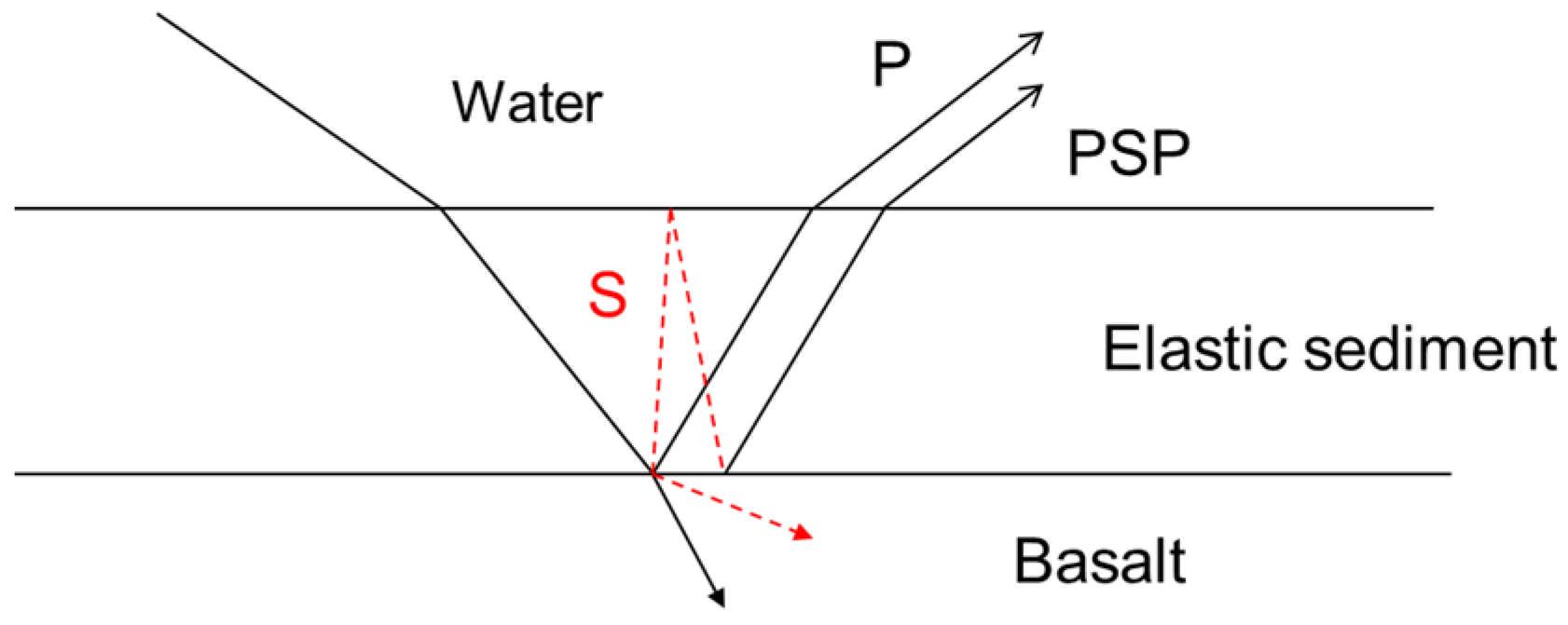
1]. An analysis of plane wave reflectivity from a thin-sediment elastic solid ocean bottom indicates two significant effects of shear waves [
25], as indicated in
Figure 1. The compressional wave that propagates through the thin sediment layer and reflects from the sediment-basalt interface (P) has additional loss owing to the shear waves that propagate in the basalt and carry energy from the incident wave. In addition, a reflection (PSP) is also generated by converted shear waves that propagate in an elastic solid sediment layer. These two reflected waves interfere in the water and generate resonances at very low frequencies that are observed in the acoustic field in the water [
25].
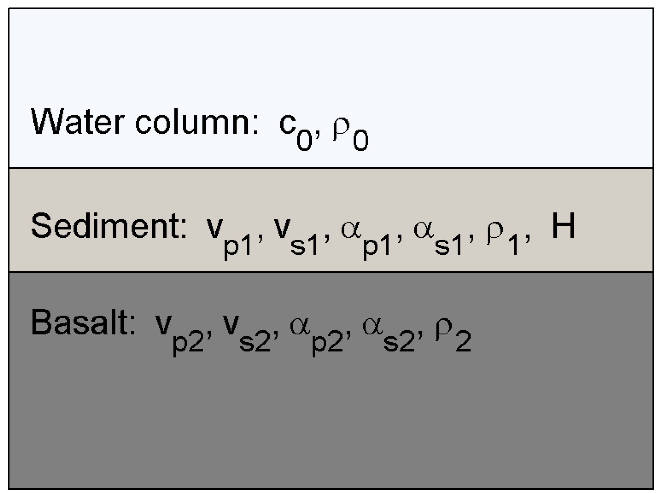
Considering the analysis of the reflectivity, an appropriate geoacoustic model for uppermost oceanic crust is a single elastic sediment layer over an elastic solid basalt basement, as indicated in
Figure 2. The model parameters in each layer are density, ρ compressional and shear wave speeds and attenuations,
vp,s and α
p,s, respectively. The sediment layer thickness,
H, is also included for a total of 11 model parameters.
Since the low-frequency reflection loss data from the experiment were primarily sensitive to the crustal layer within about a wavelength of sound (~200 to 400 m) beneath the seafloor, the geoacoustic model assumes constant sound speed in the basalt layer. This assumption is consistent with the low sound speed layer model proposed by Christeson et al. [
26] for the uppermost portion of the upper oceanic crust. If a small gradient of the sound speed did exist, the estimated results could be interpreted in terms of the average values in the layer.
3.3. Broadside Reflectivity Method
Ocean bottom reflection loss versus grazing angle data were obtained in an experiment with two ships at sites along a track from 33.38° N 131° W to 32.36° N 148.92° W in the North Pacific Ocean, roughly between the Murray and Pioneer Fracture zones. The site locations of the reflection loss experiments that are analyzed in this paper are listed in
Table 1. Water depth increased from about 5000–5500 m to the west, and crustal age increased from about 40 m.y. at the eastern end to over 70 m.y. at the western end [
27]. Ocean bottom relief in the region consisted of small abyssal hills rising 100–200 m above the sea floor and aligned at about 337° T. The sediment layer thickness was variable and very thin, around ~20 m over most of the track but increasing to ~50 m at the western end.
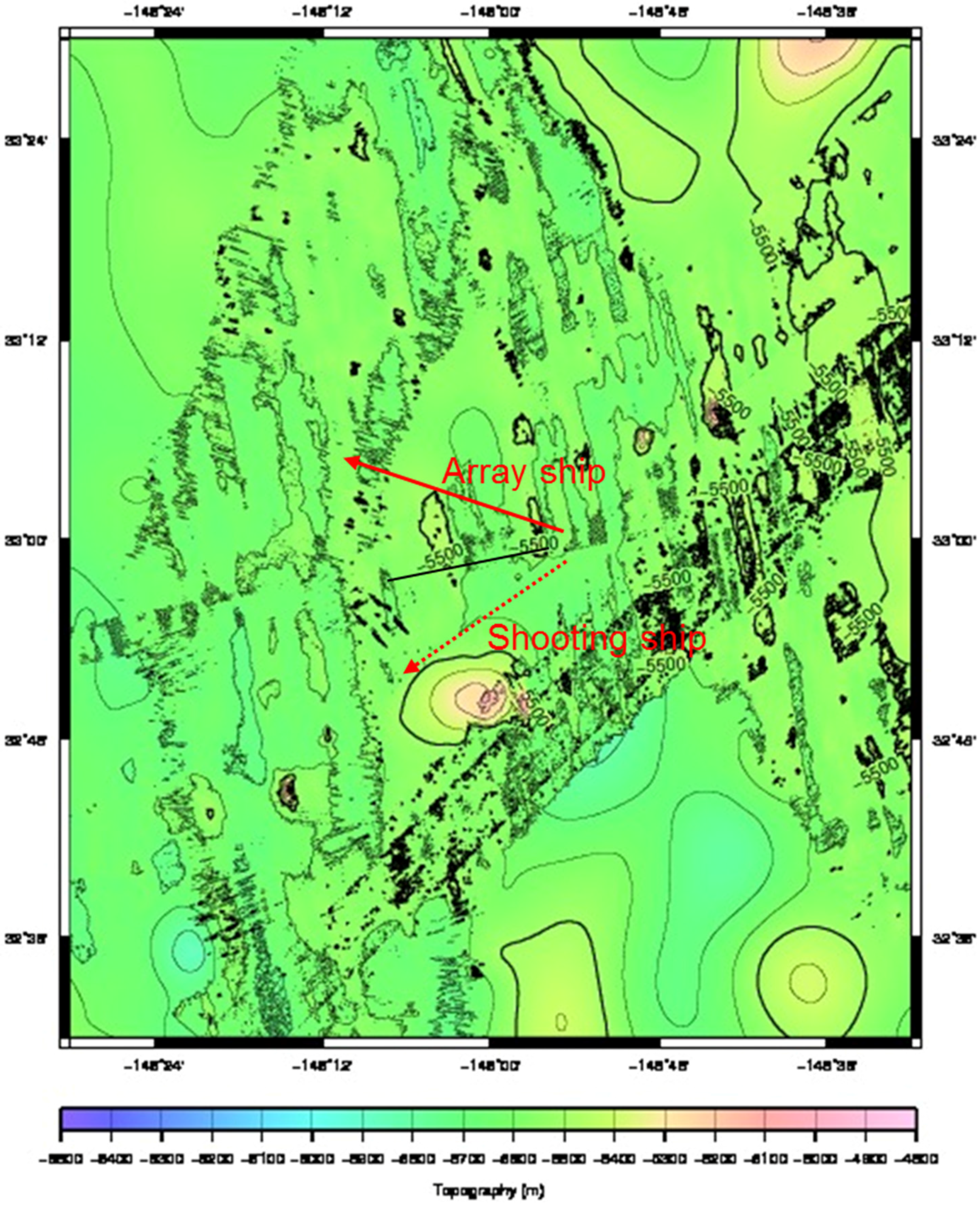
The experimental technique, the Broadside Reflectivity Method (BRM), was unconventional compared to other seismic survey methods. The shooting ship deployed 0.8 kg SUS (Signals Underwater Sound) charges at nominal depths of ~190 m on a course at each site that opened range from the receiving ship as indicated in
Figure 3 for the site at the extreme western portion of the track. The actual shot depths were obtained from measurements of the bubble pulse period of each shot. The bubble pulse data were determined from analysis of the cepstrum of the received signal [
28]. The shot signals were received on a long horizontal line array towed at a depth of ~250 m by the receiving ship. The array aperture was 1524 m with 40 hydrophone channels that were equi-spaced at 38.1 m. The array shape was monitored by six depth sensors at intervals of 310 m along the array, and the orientation and straightness were monitored by three compass sensors at the array ends and midpoint. The receiving ship also deployed shots at the start of the track at each site to obtain nominal values of the sediment thickness. The thickness was inferred from travel time analysis of the vertical incident shot data from shots that were deployed from the array ship.
The ship tracks at each site were designed so that the propagation paths of the shot signals were nearly broadside to the array for all the shot deployments. The shooting ship opened range on a course at a bearing of ~65° to the array ship’s course so that the distance between the two ships was about 35 km at the end of the ship tracks. As indicated in
Figure 3, the horizontal distance between the start and end of the ship tracks was about 20 km.
Fifty shots were deployed from the shooting ship along its track at each site, and this provided data for a set of grazing angles for the specular first bottom reflections from 80° at the initial close ranges at the start of the track to about 10° at the end of the track. Consequently, in the BRM experiment the incident point of the specular first bottom reflection on the seafloor was different for each shot. The courses and ship speeds were set so that the locus of the incident points on the seafloor covered a distance of about 20 km and was aligned perpendicular to the direction of the seafloor lineations. The incident point locus for the shots deployed at the westernmost site are indicated by the solid line between the two ship tracks in
Figure 3. Ship positions were determined from Global Positioning System (GPS) data from each ship. The shot location was determined directly from the ship position at deployment, and the receiver location was determined from the receiving ship position and a known offset to the midpoint of the array. This information was used in deriving the bottom reflection loss from the received data, and in calculating the grazing angles of the specular reflections at the seafloor.
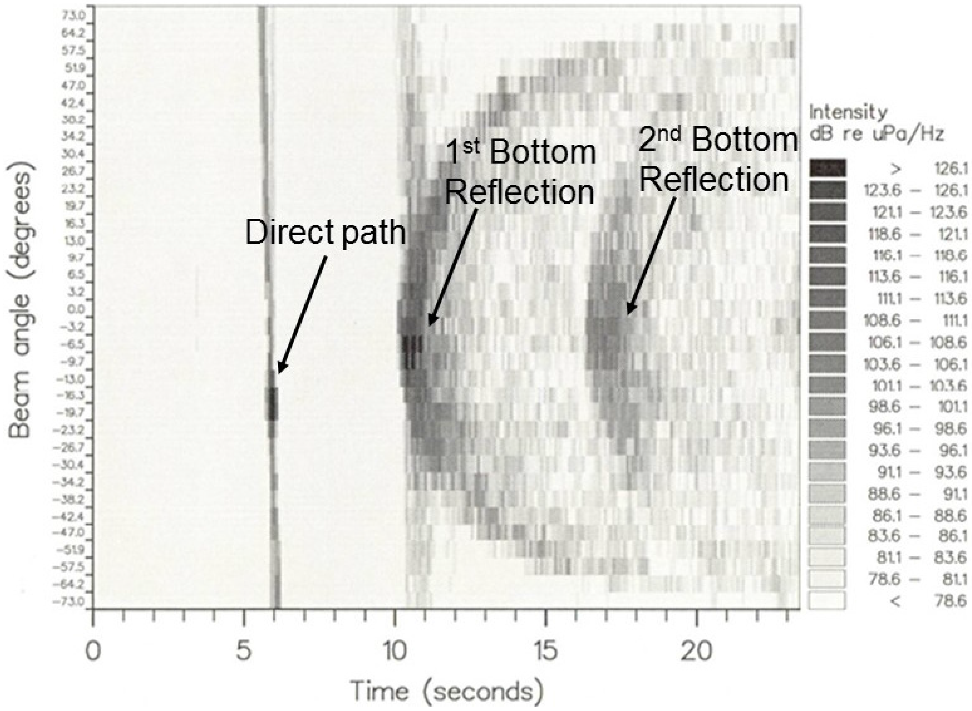
The broadband shot signals were digitized at a rate of 700 samples/s, filtered and processed by a time-delay beamformer in 1/3-octave frequency bands with centre frequencies from 8–125 Hz to obtain the array beam responses versus time for the shot signals. The bandwidth of the receiving system spanned 5–200 Hz. An example of the array data is shown in
Figure 4 for the 63-Hz band for a shot near the beginning of one of the shot runs. In deep water, the multipath signal components corresponding to the direct path and the increasing orders of bottom reflections are well resolved in time. The direct path signal is evident in the beam at ~−16° toward rear endfire, and the specular first bottom reflection, arriving approximately 4.5 s following the direct path, in the beam at ~−10°. The single bottom interacting signals that arrive at later times and at different beam angles are non-specular reflections from scattering centres on the seafloor. The second order bottom reflection is also evident, with the specular path about 11 s after the direct path in the −3° beam. The bottom reflected paths are closer to the broadside beam (0°) owing to the vertical component of the propagation paths. Signal intensity, indicated in dB re 1 μPa/√Hz, is strongest for the specular paths in each order of bottom reflection.
The beamformed data provided spatial and temporal separation of the direct path and specular first bottom reflection signals into separate beams for ranges out to ~25 km. There was significant scattering observed in non-specular beams at higher frequencies from scattering centers on the abyssal hills, but the impact of this effect was considerably reduced by using data from the specular reflection beam for the 8-Hz band in the inversions.
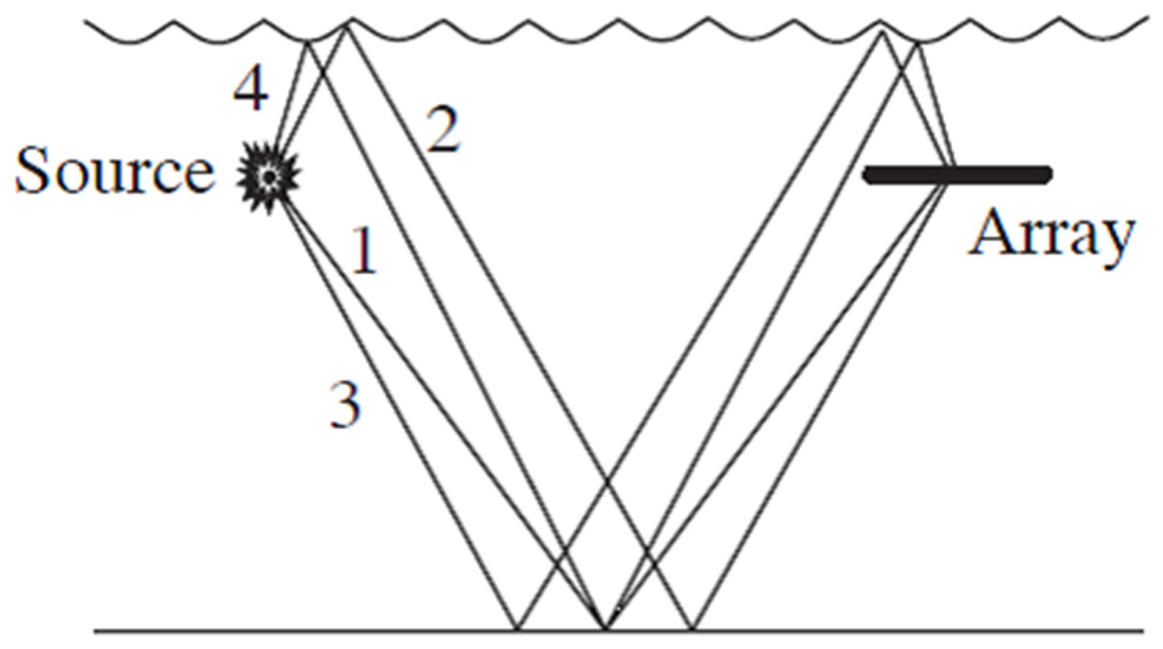
The signal in the specular first bottom reflection beam consists of four bottom-interacting paths as shown in
Figure 5. The paths correspond to the single bottom reflection path (1), two bottom interacting paths that reflect once from the sea surface (2 and 3), and the path that interacts twice with the sea surface (4). The multipath components are not resolved separately in the data, so the data used to determine the reflection coefficient consisted of the four bottom-interacting paths.
The reflection coefficient data in the 8-Hz 1/3-octave bands were derived from acoustic propagation loss measurements of the bottom-reflected signal paths. Acoustic propagation losses,
, of the signals in the specular reflection beams,
, were determined using known source levels,
, for the charges [
28] according to the equation (in dB):
The source levels were corrected for the actual shot depths that were determined from measurements of the bubble pulse periods. Bottom losses,
, were then obtained from the difference between the measured and calculated propagation losses according to:
where,
is the calculated loss, using ray theory and assuming perfect reflection at the sea floor. The calculated loss accounted for the coherent summation of the four separate bottom-interacting paths [
29]. Plane wave reflection coefficients,
, were determined from the decibel measures of bottom loss using:
Grazing angles for the specular reflection for each shot were determined by ray theory using the shot and array positions derived from the GPS data, and a sound speed profile in the water measured at each site.
Although the reflection points on the sea floor were different for each grazing angle in the BRM experiment, there was considerable overlap of the Fresnel zones on the sea floor, and the distance covered along the track at each site was only ~20 km. Consequently, the change in crustal age over the span of the measurements at each site was not significant and it was assumed that the reflection coefficient data from each site provided information about the geoacoustic properties of basalt at a well-defined age. Moreover, the interaction with the bottom was confined to within about a wavelength of the seafloor, so the data provided information about the uppermost portion of Layer 2A.
3.4. Inversion of Reflectivity Data
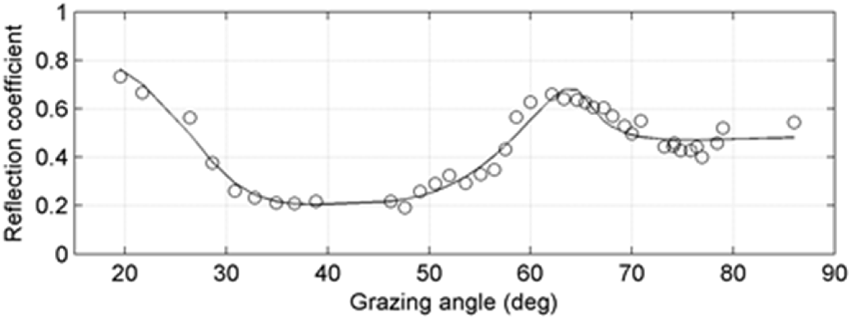
An example of the measured reflection coefficient versus angle data is shown in
Figure 6 for site 9 near the western end of the track. In this display, the raw data were smoothed using a three-point running average over angles. The most significant features of the reflection data are the peaks around 63° and 20° that are related to compressional wave and shear wave critical angles in the basalt, respectively. This indicates that the shear wave speed in the basalt is also greater than the water sound speed at the bottom at this site. However, the shear wave speeds were generally less than the water sound speed in the eastern portion of the track. For those cases, the shear wave information is contained in the magnitude and shape of the reflection coefficient versus angle data at angles less than the compressional wave critical angle.
The inversion followed the Bayesian approach outlined in Equation (12), comparing measured and modeled plane-wave reflection coefficients with the assumption that the data errors were uncorrelated and Gaussian distributed with non-identical standard deviations. The modeled plane-wave reflection coefficients were calculated in 1/3-octave bands centered at 8 Hz for each model that was tested in the inversion [
1]. The average in the 1/3 octave band was taken over 11 frequencies in the band. Prior information applied in the inversion consisted of uniform distributions for the parameter values within the bounds that are listed in
Table 2 for the 11 model parameters. The bounds were chosen to be sufficiently wide to allow the data to determine the solution in the inversion process, but at the same time limit the estimates to physically reasonable values. A compressional wave speed of 1535 m/s and density of 1.03 g/cm
3 were used for the sea bottom water.
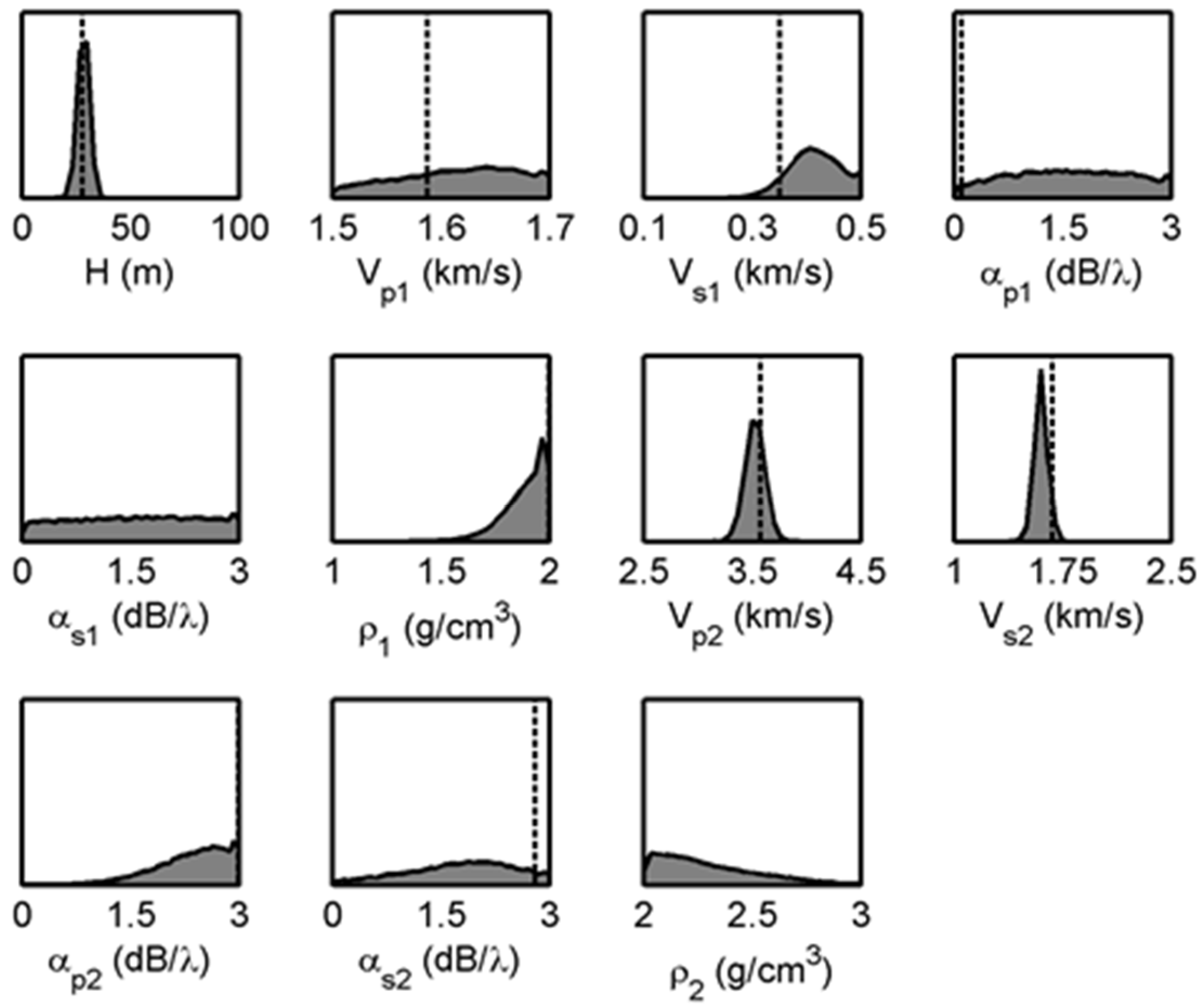
The results from the Bayesian inversion are presented in terms of one-dimensional marginal probability distributions (7) for the 11 model parameters, as shown in
Figure 7 for the data from
Figure 6. The dashed vertical line in each panel is the MAP estimate (4), for each model parameter. The most sensitive parameters are the sediment layer thickness,
H, and the compressional and shear wave speeds,
vp2 and
vs2, in the basalt, respectively. The sediment shear wave speed,
vs1, also shows some sensitivity. The marginal probability distributions for these parameters have sharp peaks within their prior bounds, indicating that these parameters are well estimated, and the MAP values also agree well with these peaks. In comparison, the marginal probability distributions for all other parameters are relatively flat, indicating that these parameters are insensitive and the reflection loss data contain no significant information about them. The results for density are also of note. The inversion tends to the upper limit for the sediment density and the lower limit for the basalt density. This suggests that the data are sensitive only to the basalt density, around 2 g/cm
3. Similar results were obtained for inversions at the other sites.
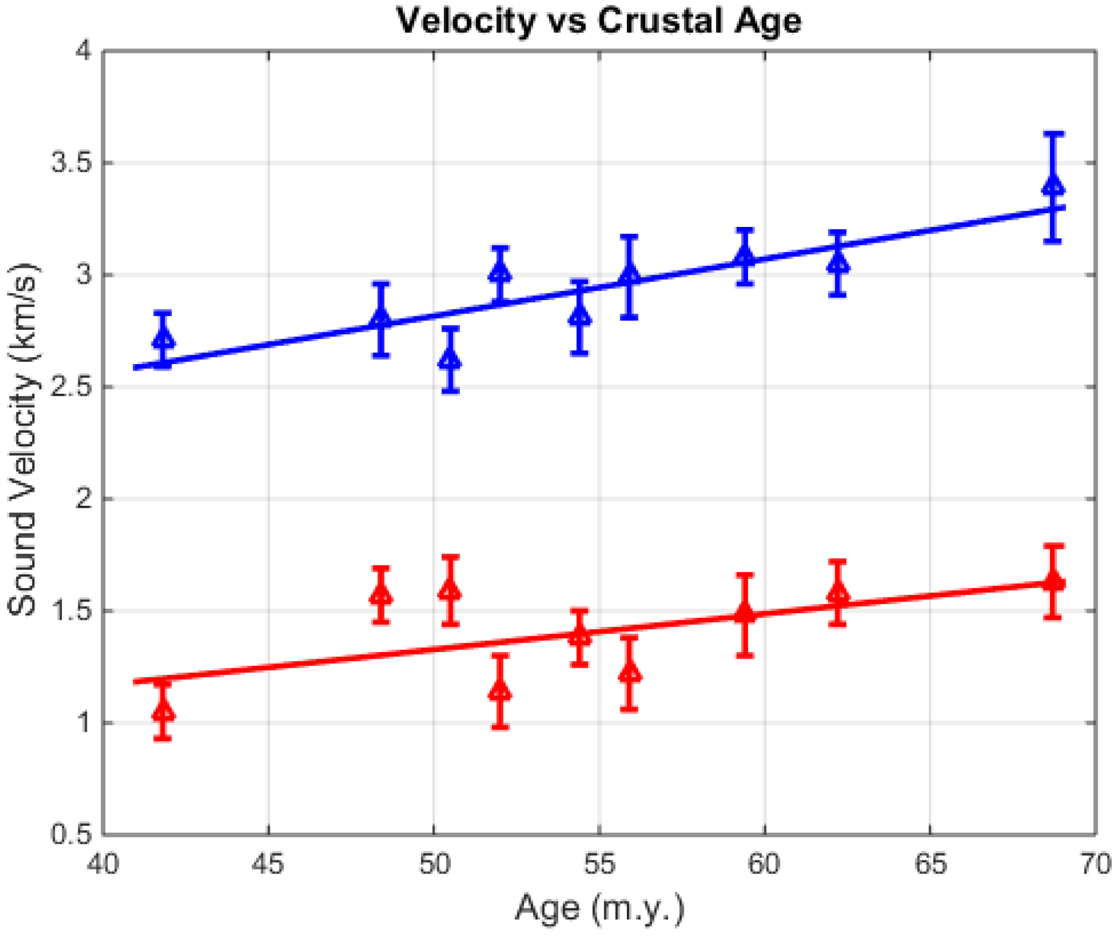
The estimated values for the compressional (P) and shear wave (S) speeds of the upper crust basalt are plotted versus crustal age in
Figure 8. A comparison is also shown in
Figure 6 of the agreement of the calculated reflection coefficient using the estimated model parameters from the inversion.
4. Discussion
This experimental technique introduced in this paper, the Broadside Reflectivity Method, is unconventional in seismic survey. The method is well designed for studying the geoacoustic characteristics of elastic solid ocean-bottom environments because it provides estimates of both the compressional and shear wave speeds. In addition, the interaction is confined within about a wavelength of sound in the bottom, so the method provides information about the uppermost part of the bottom material.
The Bayesian inversion provides estimates of the model parameters of the geoacoustic model and a measure of their uncertainties. In addition, the method indicates which of the model parameters are well estimated in the experiments. In the thin-sediment upper crust environment, the sound speeds of the basalt crust and the sediment layer thickness are well estimated. The shear wave speed of the sediment is also sensitive, by means of the resonances caused by converted shear waves at the sediment-basalt interface. Estimates are obtained for the other parameters, but the uncertainties are very large, indicating that there is weak sensitivity to those parameters in the data.
The estimated values for the compressional wave speed (P) shown in
Figure 8 are considerably less than values reported previously for upper crust of similar age but with significantly thicker sediment cover [
17]. The compressional wave speed increases slowly at a rate of about 0.026 km/s/m.y., equivalent to an increase of about 1% per m.y. This indicates that the ageing process is continuing at a relatively slow rate throughout the experimental track. The sediment thickness is consistently thin, ~20 m, for most of the track, so the conditions for hydrothermal alteration are constant. However, there is a dramatic increase in the thickness of the sediment deposit at the western end to about 50 m. The thicker sediment cover increases the insulation from ocean water and may affect the rate of hydrothermal alteration and the ageing rate at the western end. The shear wave speed (S in
Figure 8) also increases along the track, but at a slower rate of 0.016 km/s/(m.y.) The observed rates are considerably slower than ageing rates at very young crust (<3 m.y.), measured near the spreading centres where the newly formed basalt is open to hydrothermal circulation. Ageing rates of about 4.5% per m.y. were reported from experiments at the spreading centre of the Juan de Fuca ridge [
29].
Recent studies have concluded that seismic velocity in upper oceanic crust strongly depends upon the basalt porosity [
19,
30,
31]. Models of the porosity in terms of crack size distribution indicate that the presence of cracks affect the compressional and shear wave speeds differently; thin cracks tend to increase Poisson’s ratio, whereas thick cracks decrease Poisson’s ratio [
31]. From
Figure 8, it is evident that Poisson’s ratio is about 0.35 and does not change significantly over the track. Although there is no information about the porosity of the basalt, the estimated values for the sound speeds from this experiment provide constraints for models of the porosity.
A few comments are appropriate to address two issues in the measurements that affect the inversion results: the assumption of constant crustal age at each site, and scattering from the abyssal hill terrain. Crustal age increases marginally along the measurement track of about 20 km at each site. The experimental design included some intrinsic averaging of different conditions along the track since the reflection point at the sea floor was different for each shot, and also, the data were smoothed over angles using a three-point running average. Considering the reflection loss data shown in
Figure 7, the behaviour appears qualitatively consistent with the assumption of a range independent ocean bottom in which the geoacoustic model parameters, in particular the basalt sound speeds, do not vary significantly along the track of the experiment. The marginal densities for the sensitive parameters (
Figure 7) support this observation, since the distributions are very narrow. It should also be noted that temporal variability in the details of volcanic and/or hydrothermal processes within the spreading axis zone could contribute to the original velocity structure, thus affecting parameter values determined at given sites after they drifted off axis. Thus, any single value of sound speed in the overall trend suggested in
Figure 8 might shift a small amount if measured at a different detailed location of the same age.
Scattering from the crustal basalt can affect the reflectivity measured in this experiment and contribute to the scatter in the reflection loss data. Assuming that the rms roughness,
s, of the basalt interface is small, the magnitude of the scattering loss,
L, at grazing angle θ can be modeled for a Gaussian randomly rough surface by the Eckart scattering relationship [
32]:
where
,
, and
is the sound wavelength. The impact of scattering was minimized by spatial filtering the data in the specular beam of the array, and using the low frequency 1/3-octave band at 8 Hz. Since no other attempt was made to correct for scattering loss, from Equation (14) the effect is greatest at large grazing angles. At these angles, the reflection coefficient is most sensitive to the acoustic impedance contrast, so it is likely that scattering has the greatest impact on the estimate of the density. However, since the estimates of the basalt compressional and shear wave speeds are sensitive to features of the reflection loss at much lower angles, these parameters are not significantly affected.
Finally, the experiments were sensitive to the sound speed in a propagation direction aligned with the main ridge axis, i.e., along strike. There is no information from these results about anisotropy in the seismic velocities.


