Article

Application of an Unstructured Grid-Based Water Quality Model to Chesapeake Bay and Its Adjacent Coastal Ocean

Department of Natural Sciences, University of Maryland Eastern Shore, Princess Anne, MD 21853, USA
*
Author to whom correspondence should be addressed.
J. Mar. Sci. Eng. 2016, 4(3), 52; https://doi.org/10.3390/jmse4030052
Submission received: 11 July 2016 / Revised: 16 August 2016 / Accepted: 18 August 2016 / Published: 1 September 2016

Abstract

:
To provide insightful information on water quality management, it is crucial to improve the understanding of the complex biogeochemical cycles of Chesapeake Bay (CB), so a three-dimensional unstructured grid-based water quality model (ICM based on the finite-volume coastal ocean model (FVCOM)) was configured for CB. To fully accommodate the CB study, the water quality simulations were evaluated by using different horizontal and vertical model resolutions, various wind sources and other hydrodynamic and boundary settings. It was found that sufficient horizontal and vertical resolution favored simulating material transport efficiently and that winds from North American Regional Reanalysis (NARR) generated stronger mixing and higher model skill for dissolved oxygen simulation relative to observed winds. Additionally, simulated turbulent mixing was more influential on water quality dynamics than that of bottom friction: the former considerably influenced the summer oxygen ventilation and new primary production, while the latter was found to have little effect on the vertical oxygen exchange. Finally, uncertainties in riverine loading led to larger deviation in nutrient and phytoplankton simulation than that of benthic flux, open boundary loading and predation. Considering these factors, the model showed reasonable skill in simulating water quality dynamics in a 10-year (2003–2012) period and captured the seasonal chlorophyll-a distribution patterns. Overall, this coupled modeling system could be utilized to analyze the spatiotemporal variation of water quality dynamics and to predict their key biophysical drivers in the future.

Graphical Abstract

1. Introduction

As the largest and most biologically-diverse coastal plain estuary in North America [1], Chesapeake Bay (CB) is highly influenced by its vast watershed with a land-to-water ratio of 14.3 [2]. Following the population growth, industrial and agricultural development, CB has undergone severe eutrophication with symptoms of excessive nutrient loading, nuisance algal blooms, extensive summer hypoxia and declined seagrass coverage since the mid-1900s [3,4]. Typically, the overloading of cultural nutrients into CB directly drives its water quality deterioration, including bottom hypoxia/anoxia, overwhelming phytoplankton growth and diminished water clarity [2].
Biogeochemical cycles in CB and similar water bodies have been investigated using field investigation [5,6,7], retrospective long-term data analysis [8,9], remote sensing images [10], and numerical simulations [11,12]. Intra-seasonal and inter-annual observed data can effectively detect the dominant environmental factors driving water quality variations, but is usually limited by sparse spatiotemporal resolution [13]. Satellite imagery provides synoptic surface phytoplankton and suspended material distribution while it is incapable of exhibiting vertical variation [10]. Statistical empirical models and simplified oxygen models omitting nutrient cycles have been developed as substitutes for specific research goals, but it is impossible to reproduce the detailed internal spatiotemporal water quality variation and comparatively evaluate biophysical drivers [14]. In contrast, the three-dimensional physical-biogeochemical model could better resolve the biophysical interactions between circulation and water quality kinetics [11,12] and facilitate mechanistic analysis of internal water-column dynamics [15,16,17], making it an ideal tool to investigate nutrient dynamics and algal variability in eutrophic estuaries [18], synoptically assess estuarine biophysical processes and project future scenarios [19,20].
However, there exist several challenges and limitations in developing and applying sophisticated biophysical models [20]. For example, low-resolution models have difficulty following the coastline or investigating the tributary-estuary exchange very well. Unstructured grid models have the advantage of flexibility reaching fine resolution at areas of interest (e.g., nearshore, sills, deep channels and fronts) over the structured grid models [21]. Other key challenges and sources of uncertainty in configuring biophysical models lay in meteorological forcing, hydrodynamic simulation and nutrient loading [20]. For example, turbulent mixing and bottom roughness are key factors for the bay circulation [22], while their effects on the water quality dynamics are less investigated. In addition, uncertainties and errors originating from these processes have been poorly compared and discussed in any biophysical model application, and these limitations could be magnified when modeling a biologically-diverse estuary (e.g., CB) and cause biases when interpreting the model simulations and providing management suggestions [12,23].
Since high resolution would potentially benefit the water quality simulation, a three-dimensional biophysical model was configured for CB, its tributaries and adjacent coastal ocean based on the unstructured grid modeling framework FVCOM-ICM [24], which comprises the hydrodynamic model, the finite-volume coastal ocean model (FVCOM) and a water quality component, the modified Corps of Engineers Integrated Compartment Water Quality Model (FVCOM-ICM, [24]). During the model development, we tried to achieve a comprehensive understanding of various uncertainties for the model development and answer the following questions: (1) how will increased model resolution improve the simulation of water quality variables; (2) how sensitive is the model to different wind sources; and (3) what is the most significant physical and biological sources of uncertainty in our model? Section 2 and Section 3 introduce the model frame and sensitivity experiments; model calibration results are depicted in Section 4; Section 5 lists the major conclusions.

2. Material and Methods
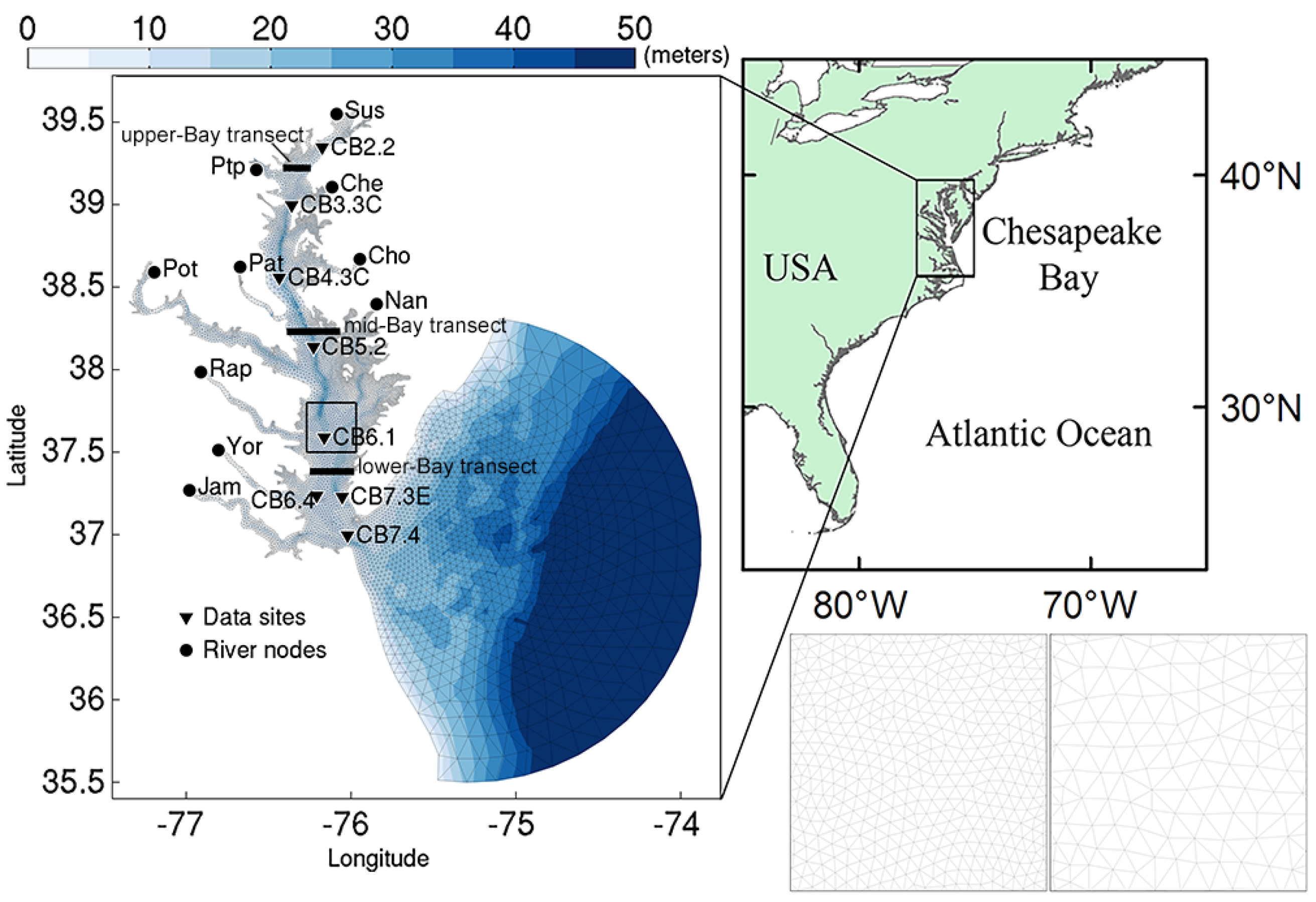
2.1. Study Site

CB, located adjacent to the Mid-Atlantic Bight on the east coast of United States (Figure 1), is a partially-mixed drowned river valley with a residence time of 90–300 days depending on the river flux [2,25]. A deep channel in the middle and shoals on both flanks (Figure 1 [2]) characterize the main stem of this large estuary with an area of 11,600 km2 (323 km long, 48 km wide and 6.5 m deep on average), where the salinity typically ranges from 0–30 from the northern to the southern end. A two-layer estuarine circulation is subject to variation in river flux, local/remote winds, semidiurnal tides and other forces [26,27]. Receiving 337.3 kt/year (kt = thousand tons) nitrogen and 23.7 kt/year phosphorus inputs by 2010 [28], CB generates 2–12 km3 bottom hypoxic waters every summer [29] and witnesses frequent occurrence of harmful algal blooms [30], which threatens the bay’s living resources and ecological service to its recreational and commercial users.

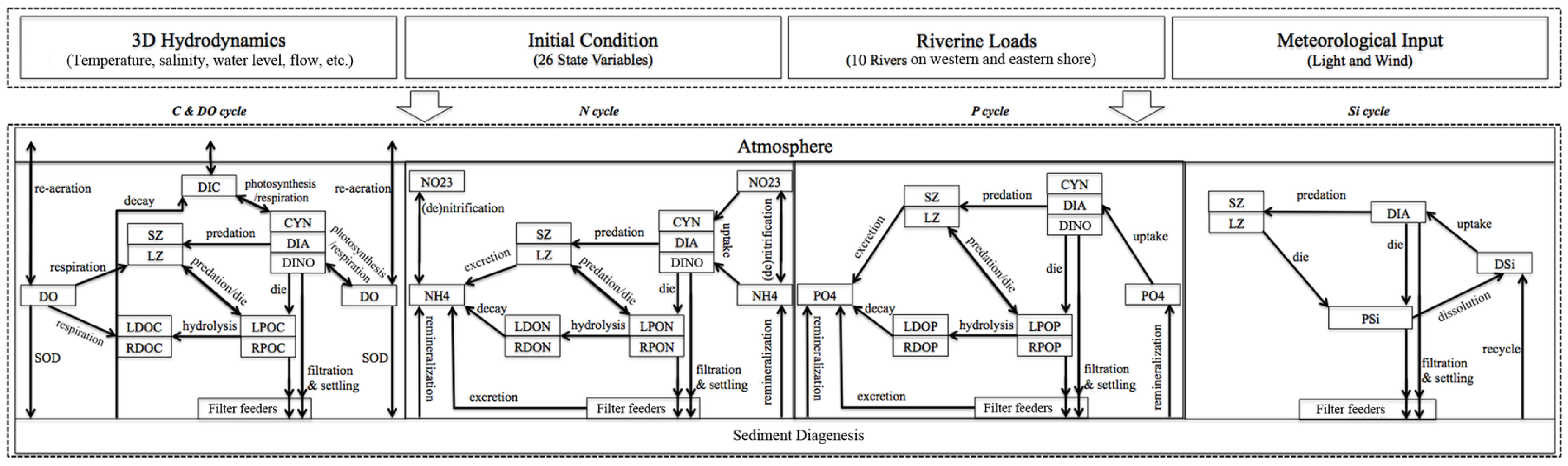
2.2. Model Description

An unstructured grid FVCOM-based hydrodynamic model was used to simulate the water level, temperature, salinity, circulation, eddy viscosity and other hydrodynamic information at an external and internal time step of 3 s and 12 s, respectively [31]. This work adopted this existing hydrodynamic model with the grid size ranging from 270 m–20.9 km (Figure 1). The major external forcing was comprised of daily river discharge, atmospheric forcing and open boundary conditions. The hydrodynamic data sources, calibration and validation processes and the justification of model settings could be retrieved in detail from [31].
The water quality kinetics, including nutrient cycles, sediment diagenesis and plankton growth, was simulated in the FVCOM-based water quality model FVCOM-ICM [24]. Integrated Compartment Model (ICM) was originally developed for the CB restoration and now works as part of the predictive model package CBEMP for the total maximum daily load plan [11,28]. A primary difference between CBEMP and FVCOM-ICM is our use of the unstructured grid and the sigma coordinate to accommodate the complex bay coastline and bathymetry. The mass balance of state variables in each control volume/cell [11] is solved as follows.
V C t = k = 1 n Q k C k + k = 1 n A k D k C x + V S
In Equation, V is the volume of a cell (m3), C is the concentration or biomass in the cell (mg/L), t is the temporal coordinate (s), Qk is the flux across the interface with the k-th neighbor cell (m3/s), Ck is the concentration or biomass across the interface between two cells (mg/L), Ak is the interface area (m2), Dk is the diffusion coefficient at the interface (m2/s), n is the number of neighbor cells, i.e., the number of interfaces, x is the spatial coordinate (m) and S is the changing rate due to external loads and kinetic reaction in the cell (mg·L−1·s−1). To adapt to the sigma (σ) coordinate system, the transport of each state variable is modified as below [24].
C D t + C u D x + C v D y + C ω σ = x ( A h H C x ) + y ( A h H C y ) + 1 D σ ( A v H C σ ) + D S
In the equation, D is total depth (H + ζ, m), where H is the mean water depth and ζ is the water elevation, Ah is the horizontal diffusivity (m2/s), Av is the vertical diffusivity (m2/s), u, v and ω are velocity components (m/s) in the directions of x, y and σ, respectively, and S is the biogeochemical changing rate (mg·L−1·s−1).
We simulated a total of 26 state variables in carbon, nitrogen, phosphorus, silicon and dissolved oxygen (DO) cycles (Figure 2), including total suspended solids (TSS), cyanobacteria, diatoms, dinoflagellates, microzooplankton (20–200 μm), mesozooplankton (0.2–20 mm), ammonia (NH4), nitrite and nitrate (NO23), phosphate (PO4), particulate inorganic phosphorus (PIP), labile/refractory dissolved/particulate organic carbon (LDOC, RDOC, LPOC, RPOC), labile/refractory dissolved/particulate organic nitrogen (LDON, RDON, LPON, RPON), labile/refractory dissolved/particulate organic phosphorus (LDOP, RDOP, LPOP, RPOP), chemical oxygen demand (COD), DO and particulate/dissolved silica (PSi/DSi). The sub-models of sediment diagenesis [32] and bivalve filtration [33] were turned on. ICM in CBEMP showed considerable model skills in representing the water quality variables for decades [11], so most of their model settings and parameters were followed (Table 1).
We simulated three major phytoplankton groups in CB [6]: diatoms (including other winter/spring groups), dinoflagellates (including other summer species) and cyanobacteria. Dinoflagellates were treated as autotrophs with their grazing capability not modeled. The time-dependent phytoplankton biomass governing equation [11] is given below.
B t = ( G R ) B W B z F z B Z F B
In the equation, B is the biomass of a phytoplankton taxon (mg/L), G and R are the growth and respiration rate, respectively (day−1), W is the settling velocity (m/day), z is the vertical coordinate converted from σ levels (m), Fz (L·mg−1·day−1) and F (day−1) are the predation rate of zooplankton and other herbivores, respectively, and Z is the zooplankton biomass (mg/L). The growth rate is a function of temperature, nutrients and light, while the respiration rate is simply dependent on temperature. Equation (4) [11] is the depth-integrated net primary production (NPP) to manifest the detailed growth and respiration calculations.
N P P = ( ( P m C C h l I I 2 + I k 2 N K h + N e K T ( T T O P T ) 2 ) ( 1 P r e s ) M e K T ( T T r e f ) ) G d z d t
In the equation, Pm is the maximum photosynthetic rate (day−1), CChl is the carbon to chlorophyll ratio, I and Ik are the instantaneous and reference radiation (mol·photons·m−2·day−1), N is the concentration of each nutrient (nitrogen, phosphorus and diatom-only silicon, mg/L), Kh is the half-saturation concentration in the Michaelis–Menten nutrient limitation function (mg/L), KT (°C−2) and KT (°C−1) are the temperature coefficients on photosynthesis and basal respiration, respectively, Topt and Tref are their corresponding optimal and reference temperature (°C), Pres is the percentage of active respiration in gross primary production and M is the basal respiration/metabolism rate (day−1).
The light attenuation process is calculated with a subroutine computing the coefficient of diffuse light attenuation Ke (m−1), which is controlled by the scattering and absorption to suspended solids and chlorophyll in the water column. In FVCOM-ICM, a look-up table along the visible spectrum (400–700 nm), derived based on field measurements in CB, is created to determine the six independent parameters, which feeds the subroutine for Ke calculation. The formulation and description of the light attenuation subroutine are detailed in [11,21].

2.3. Model Settings

For the simulation period 2003–2012, FVCOM-ICM off-line reads hourly hydrodynamic information from FVCOM. When the 30-min time interval in the water quality model was applied, simulated water quality variables reached over 90% correlations with those with a 5-min interval, while the computational time is only 22.4%; so we conducted water quality simulations at a time step of 30 min. We included 10 major riverine boundaries (Figure 1) for nutrient and TSS loading. The monitoring nutrients, TSS and phytoplankton maintained by the EPA Chesapeake Bay Program (CBP [36]) were the main data source of our model initialization, calibration and validation. The point-source and nonpoint-source loading of carbon, nitrogen, phosphorus and TSS were from the CBP’s watershed model, Hydrological Simulation Program in Fortran (HSPF) in Phase 5.3.2 [36]. The deposition of nitrogen and phosphorus from the air-sea surface were estimated based on the observations (Stations MD13, MD15, MD99, VA10 and VA98) from National Atmospheric Deposition Program [37]. We referred to the monthly World Ocean Atlas 2005 data [38] for setting open boundary conditions. Meteorological data were downloaded from the National Center for Environmental Prediction (NCEP), North America Regional Reanalysis (NARR [39]). After model setup, major parameters were calibrated among literature ranges (Table 1) with data of 2010 to achieve the most reasonable and reliable model performance and verified with the other nine years’ data. In order to validate our eutrophication model, we also compared our simulated chlorophyll-a (CHLA) distribution with the remote sensing images from the Chesapeake Bay Remote Sensing Program [40].
As suggested by Fitzpatrick, we computed the correlation coefficient (CC; Equation (5)) and the root mean squared error (RMSE; Equation (6)) to evaluate the fit between predicted (Pi) and observational (Oi) dissolved inorganic nitrogen (DIN) and phosphorus (DIP), TSS, DO and CHLA.
C C = i = 1 n ( O i O ¯ ) ( P i P ¯ ) i = 1 n ( O i O ¯ ) 2 i = 1 n ( P i P ¯ ) 2
R M S E = i = 1 n ( P i O i ) 2 n

2.4. Design of Numerical Experiments

In order to quantify the uncertainties in both hydrodynamic and water quality sub-models, we performed a variety of sensitivity tests along with the model calibration process (Table 2). These experiments were designed using the year 2010, which has been calibrated and has normal meteorological and hydrological conditions [31,41]. The effects of grid resolution on water quality simulation were examined using two model experiments with different spatial resolutions (the average grid size inside the bay is 1.43 km versus 1.74 km, respectively; see Figure 1). We also compared the water quality simulations with six, 11 and 21 sigma levels to determine the optimal vertical resolution. Given that the water quality simulation is sensitive to vertical mixing and bottom shear [20], the impacts of varied vertical eddy viscosity and bottom roughness length scale (Table 2) were discussed based on the calibrated hydrodynamic model [31]. We also examined the controls of two spatially-varying wind sources, NARR (spatial resolution of 30 km) and observation (data from 39 stations from National Data Buoy Center [42] and the National Centers for Environmental Information [43]), on DO variation. For the boundary loading, we altered the nutrient input from various sources (riverine, benthic and open boundary) to understand their influence on primary production. Additionally, the predation of zooplankton and suspension feeders was turned on and off to examine their controls on phytoplankton prey, respectively.

3. Sensitivity Experiments

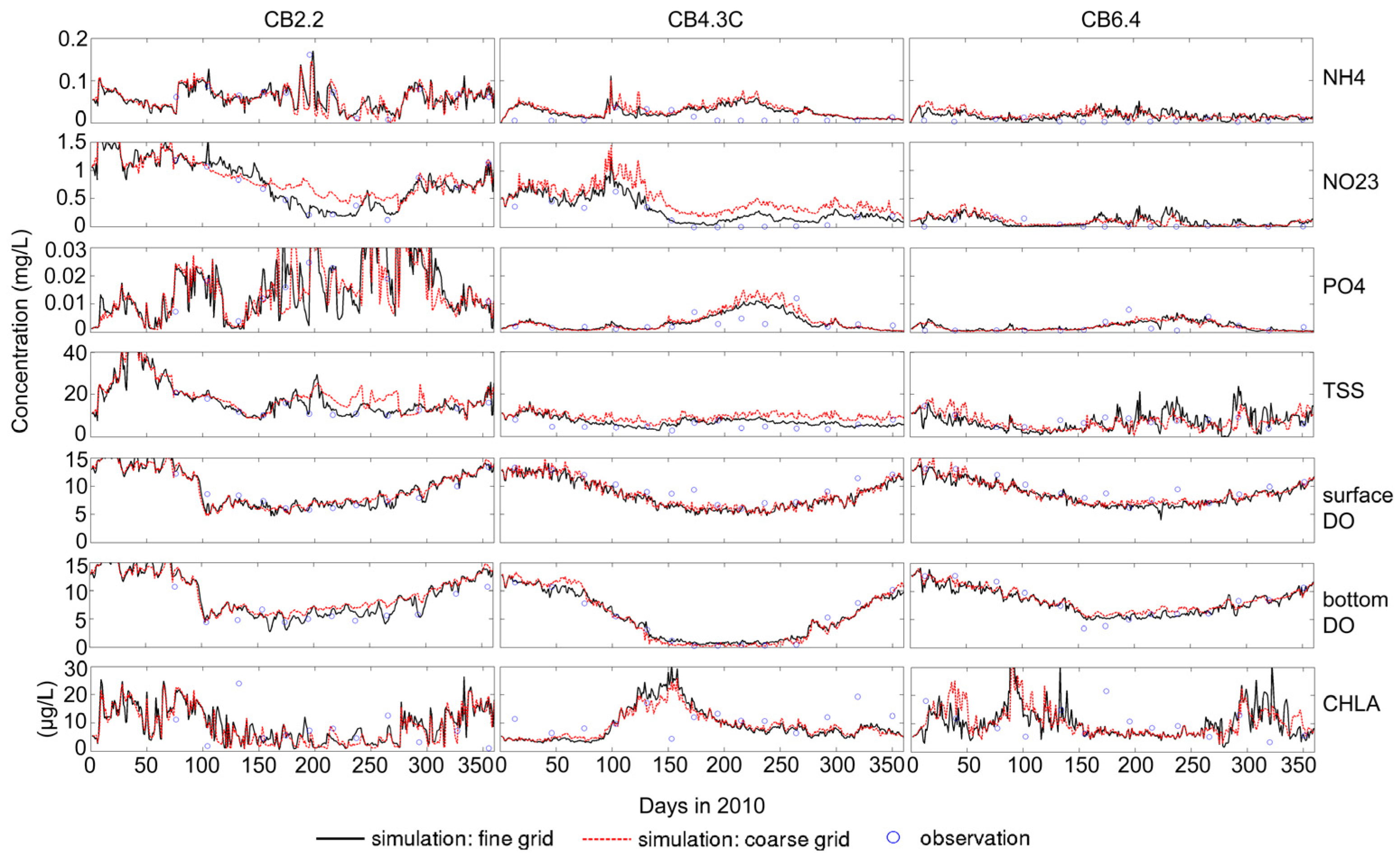
3.1. Sensitivity of Main Water Quality Variables to Grid Resolution

3.1.1. Effect of Horizontal Resolution

Two sets of model grids using different resolutions were applied in order to compare their performance and determine the optimal grid size. In the water quality simulation of 2010, both simulations represented the seasonal variation of nutrients, TSS, DO and CHLA at three stations located at the upper, middle and lower bay (Figure 1 and Figure 3). Nitrogen, TSS and CHLA peaks appeared to be associated with the high-flow period in spring, and the concentration/biomass decreased with the distance from the northern end. Strong water-column and sediment respiration, as well as the low solubility in summer lowered the oxygen level at both the surface and bottom, and the lack of strong mixing ventilation contributed to the depletion of bottom oxygen at the upper and middle bay. Hypoxic conditions at the sediment-water interface favored the release of regenerated ammonia and phosphate, causing the “bump-ups” of their concentrations. The annual cycles of simulated nutrients, TSS, DO and CHLA by both models are in line with what were previously observed in CB (e.g., [5,29,35,44]).
However, there was discrepancy between them. For instance, the nitrate concentration in the low-resolution model was higher than that of the high-resolution one at the upper-bay and mid-bay stations, particularly in late spring and summer; the difference in phosphate concentration reached around 0.003 mg/L at the mid-bay station in summer; TSS simulation was also impacted by the model resolution at the upper and middle bay. It was found that the model performance of all water quality variables was better in the fine-grid model, as revealed by higher correlation coefficients and lower root mean squared errors, and that DIN and TSS were among the variables with a large deviation between the two models (Figure 4 and Table 3). Given that model resolution impacted simulating circulation [31], the discrepancy in these two variables with a strong axial gradient along the bay was probably attributable to the along-bay transport processes, which was substantiated subsequently.
Thus, we calculated the freshwater delivery (Equation (7)) across transects at the upper, middle, and lower bay, which, not influenced by the biological processes, represented the downstream transport capacity of the riverine source at these portions of the estuary.
Q f v = v Δ S S 0 d A
In the equation, v is the southward velocity, S0 is the density of ambient water, ΔS is the density difference with the ambient water and A is the cross-sectional area. Time series of the freshwater transport at the upper bay resembled that of nitrate and TSS (Figure 1, Figure 3 and Figure 5), which supported our conclusion that circulation was responsible for improved water quality simulation in the high-resolution model. During the relatively dry summer, the freshwater transport of the coarse-grid model was higher across the upper-bay transect than the fine-grid model, but slightly lower across the mid-bay transect (Figure 1 and Figure 5). That is, more riverine nutrients and TSS were retained between these two transects (e.g., the station CB4.3C), which further supported the relationship between the physical transport and water quality simulation. In addition, the freshwater transport through the lower-bay section calculated in the coarse-grid model fell short of that in the refined model (Figure 1 and Figure 5), and as a result, the nitrate and TSS, whose major sources were the upstream riverine inputs, were lower at the lower-bay station CB6.4 in the low-resolution model (Figure 3).
Therefore, the refinement of spatial resolution improved the simulation of axial material transport along CB and the corresponding water quality variability. Using the high-resolution model, the CCs of DIN and TSS could increase by 10%–25%, and the RMSEs decrease by over 60% (Figure 4), so we adopted the refined model to conduct the following sensitivity tests.
Even though not quantified, the previous findings [14,45] were similar pertaining to model resolution. Namely, more realistic physical processes were resolved in higher-resolution model, which will in turn improve the model performance of water quality variables in both freshwater and coastal systems [14,46]. When a finer model grid is necessary, a structured-grid model usually requires increasing the spatial resolution of the whole domain or applying the sometimes problematic model nesting methods [24]. Thereby, the extensive application of high-resolution unstructured grid water quality models is highly recommended given their flexibility in regional model refinement at relatively low computational cost. However, many other factors should be taken into consideration when refining the regional mesh size; for example, high resolution may lead to errors in sub-grid-scale processes, alteration of parameterization [45] and declined computational efficiency (e.g., the computational time decreased ~28% when the coarse grid was used).

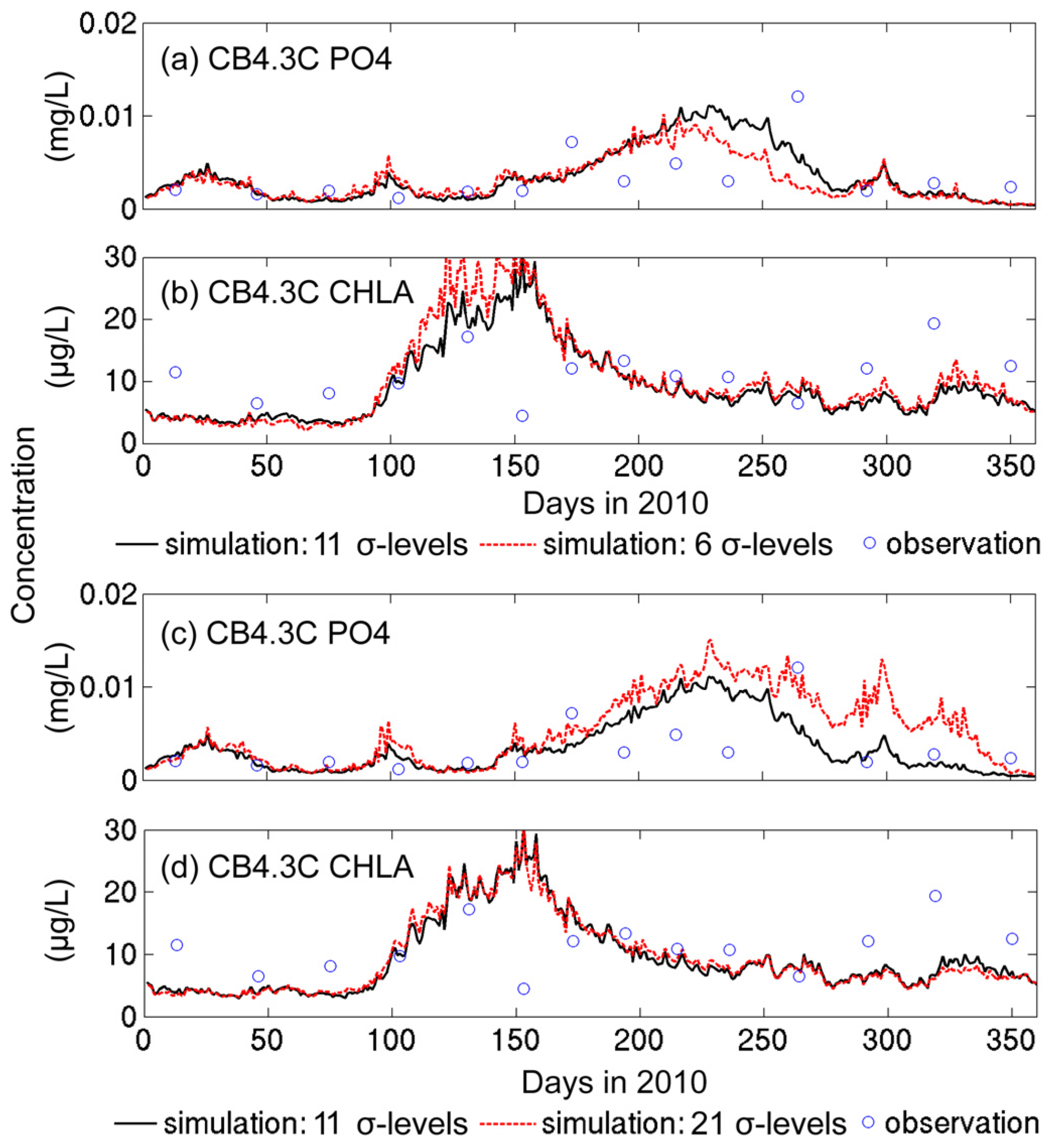
3.1.2. Sensitivity to Vertical Resolution

We applied six, 11 and 21 sigma levels to examine the response of water quality variables to vertical resolution. The sensitivity of vertical resolution was not as high as that of the horizontal resolution, and DIP and CHLA are among the most sensitive variables in comparison with the observational data. For example, at the productive mid-bay station CB4.3C, the model with six sigma levels underestimated the phosphate concentration by up to 0.005 mg/L in summer (Figure 6a) and overestimated the peak CHLA by up to 10 μg/L during the spring bloom compared to the model with 11 sigma levels (Figure 6b); in contrast, the difference between models with 11 and 21 sigma levels was not as significant (Figure 6c,d). The model with 21 sigma levels has the highest model-observation agreement for DIP (CC = 0.642 and RMSE = 0.014), while the model performance of CHLA simulation was highest in the 11-sigma-level model (CC = 0.480 and RMSE = 7.516).
The simulated hydrodynamic and water quality differences between the 11-sigma-level and 21-sigma-level model were quantified along and across the bay. The difference of salinity in the highly-productive May was mostly within one; the DIN discrepancy was maximized on the western flank and was mostly within 0.2 mg/L; phytoplankton biomass with 21 sigma levels exceeded that of the 11-sigma-level model by up to 0.1 mg/L, especially in the lower bay and on the eastern flank; the DO difference was around 0.4 mg/L throughout the water column (Figure 7). Thus, the overall model results of 11 sigma levels were similar to that of 21 sigma levels, while the difference from the six-sigma-level model was relatively large, which was also found in the CB hydrodynamic simulation [31]. In addition, the computational time of the models with six and 21 sigma levels was 54.6% and 194.0% that of the 11-sigma-level model, respectively. In consideration of the above results and the relative computational efficiency, we applied 11 sigma levels for further analyses.
When determining the vertical resolution in water quality models, it is essential to consider, but not be confined to, the overall depth, vertical circulation of the system, purpose of study and the acceptable computational expense. For instance, ten sigma layers were sufficient to simulate the seasonal nutrient cycle in Puget Sound whose maximum depth was over 200 m [21]. Conducting sensitivity tests on sigma levels could help detect the potential problems of low resolution and save the unnecessary computational time running high-resolution models.

3.2. Uncertainties Associated with the Hydrodynamic Simulation

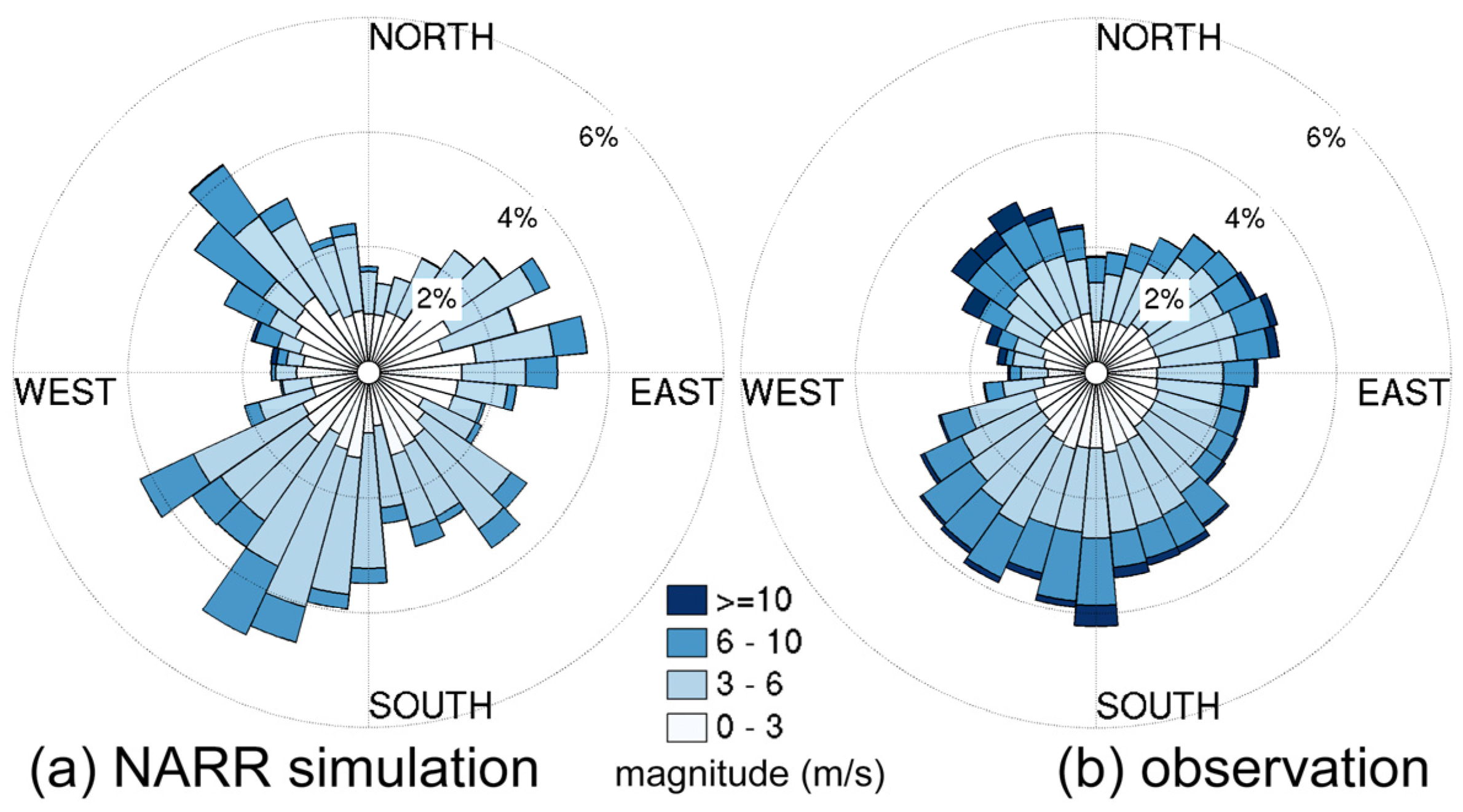
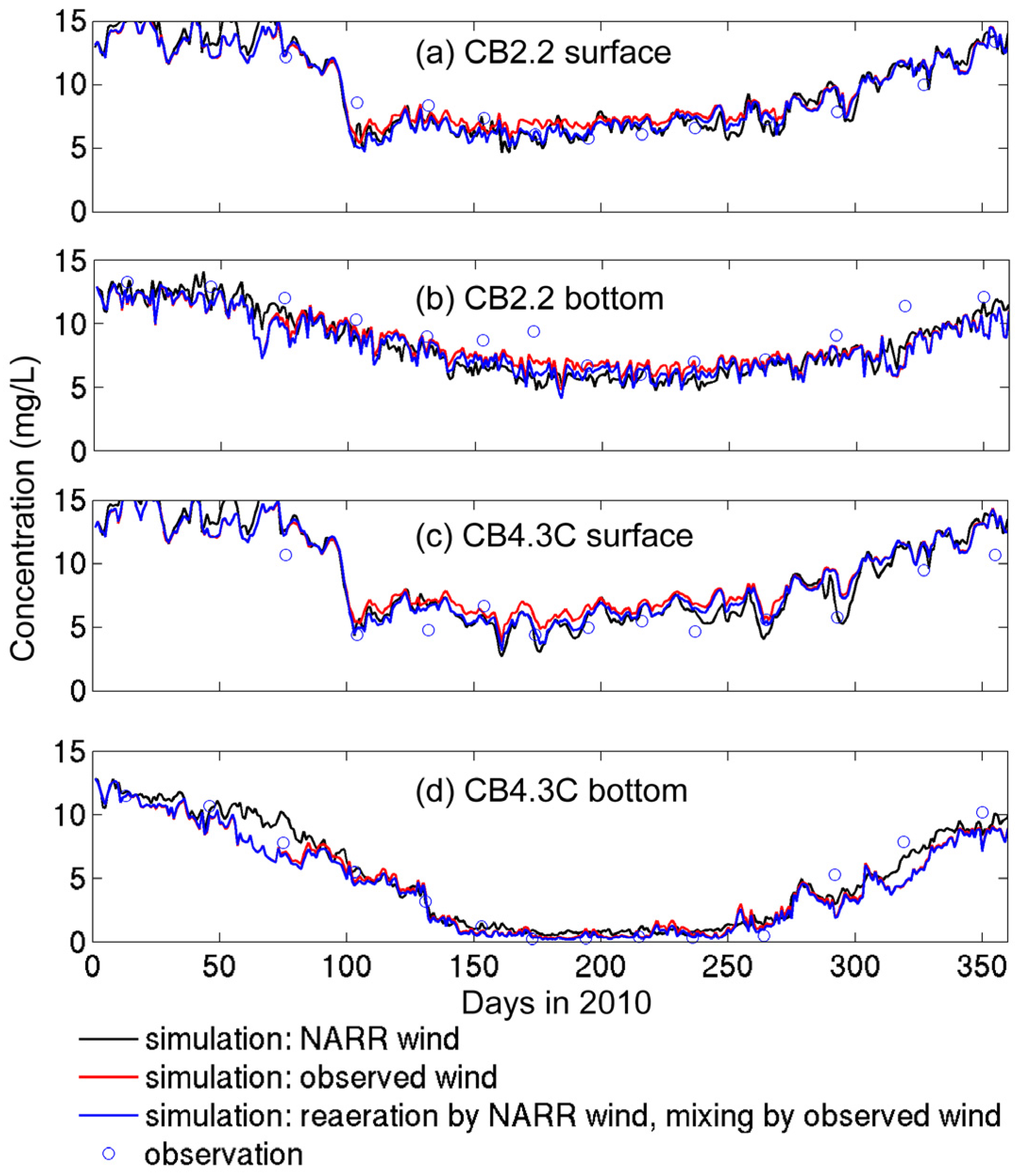
3.2.1. Sensitivity to Different Wind Datasets

Two main sources of winds over the study area are the NARR and observed data, which were applied to several studies of DO simulation [12,15,47,48]. Scully [48] claimed that the usage of measured wind displayed asymmetry in strength (strongest from the south and weakest from the west) in summer. The wind rose diagrams from May–August in 2010 revealed that both winds showed the aforementioned asymmetry, while the southerly wind was more frequent in the NARR simulation (Figure 8). The model performance of DO simulation under the observed winds (CC = 0.823 and RMSE = 1.957) was close, but inferior to that driven by the NARR winds (CC = 0.892 and RMSE = 1.525, Table 3).
At the upper- and mid-bay stations CB2.2 and CB4.3C, simulations forced by both winds exhibited similar DO reproduction, except that the DO concentration under the observed winds was slightly overestimated, particularly at the surface (Figure 9). In addition, the scenario under the observed wind underestimated DO by 2–3 mg/L in spring and fall at CB4.3C (Figure 9d). In the scenario with the mixing process driven by the observed winds and the reaeration process driven by the NARR winds, DO time series at both stations were similar to that under the observed winds (Figure 9), which indicated that the difference of two wind sources was primarily attributable to the mixing process instead of the wind-driven reaeration. Namely, the lower vertical mixing due to less frequent southerly winds accounted for the overestimation of surface DO in summer and the lower overall model skill of DO simulation. Thus, we adopted the NARR wind data for the 10-year simulation and sensitivity tests.
Winds can exert a substantial control on the onset, development and elimination of summer hypoxia in CB, and wind-driven lateral circulation and mixing may induce the ventilation of the bottom waters [49]. In other systems, wind could modulate the DO advection by direct entrainment [17,18]. Increasing the spatial resolution of observed winds and reducing data gaps might improve the DO simulation in water quality models.

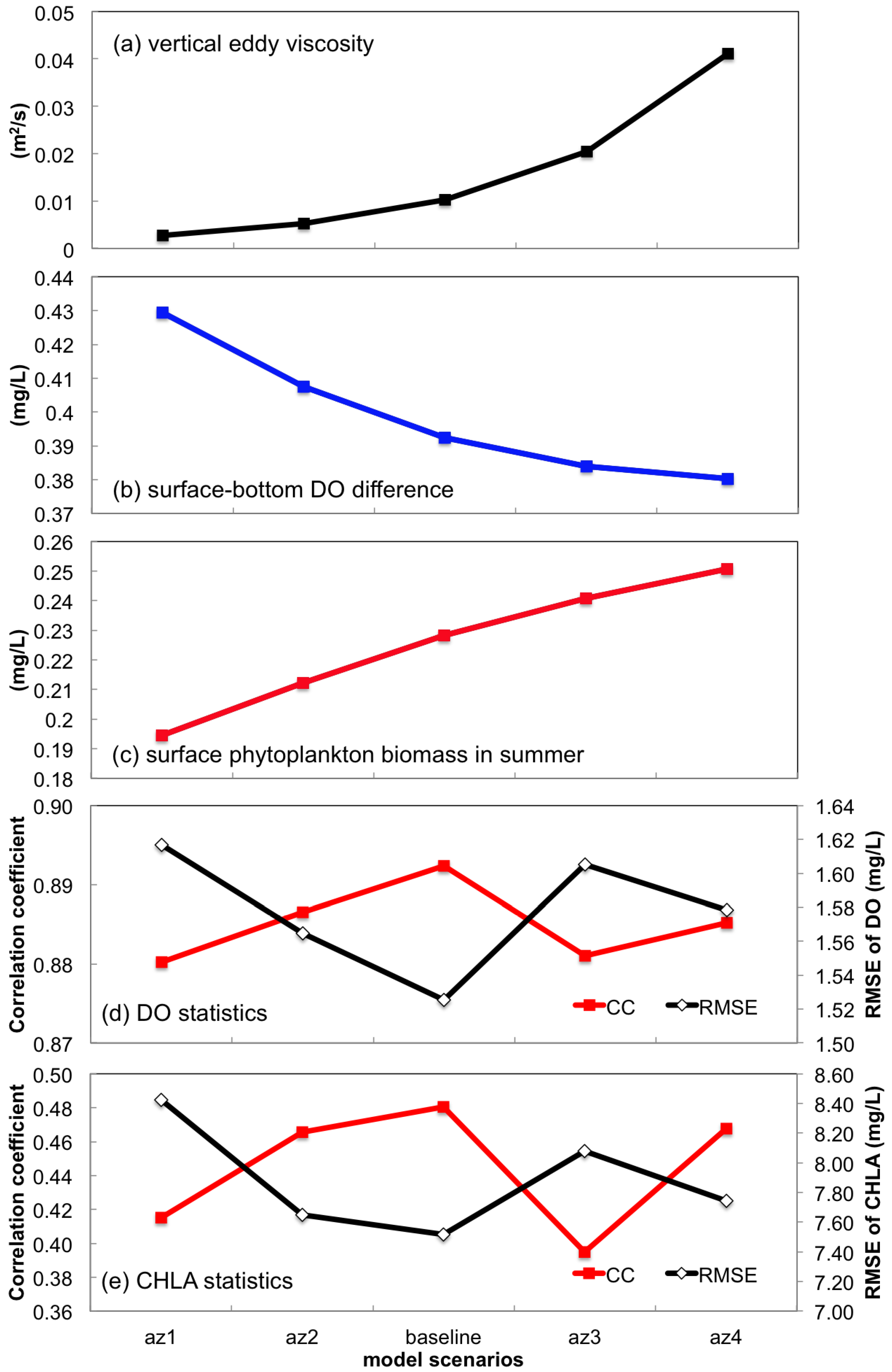
3.2.2. Sensitivity to Vertical Eddy Viscosity

Since FVCOM-ICM used the turbulence closure process from the hydrodynamic model, vertical eddy viscosity was a key coupling parameter between hydrodynamic and water quality models [24]. In our sensitivity experiments, we adjusted the vertical eddy viscosity by altering the Prandtl number. The baseline scenario was from the calibrated hydrodynamic model [31], and four other scenarios showed roughly 25%, 50%, 200% and 400% of the eddy viscosity in the baseline case (Table 2 and Figure 10a).
With enhanced mixing, the vertical DO difference in summer steadily declined at the inner bay, indicating an enhanced vertical exchange of oxygen (Figure 10b). When turbulent mixing was reduced from the baseline case, i.e., under the az1 and az2 scenarios (Table 2), the vertical difference was more sensitive to eddy viscosity, as revealed by a larger DO difference, than the two other scenarios (Figure 10b). Of all of the cases, the baseline scenario rendered the highest correlation with the observed DO and lowest deviation (Figure 10d). Therefore, the appropriate representation of turbulent mixing could improve the simulation of DO vertical exchange, as also suggested by Irby et al. [23].
Besides vertical ventilation of oxygen, the surface phytoplankton biomass was positively related to the eddy viscosity in summer (Figure 10c), which implied that the algal growth was limited by the amount of regenerated nutrients delivered to the surface. The nutrient cycling should be largely influenced by the extent of turbulent mixing, and this finding was consistent with the field study by Malone et al. [35]. Similarly to DO results, the baseline scenario exhibited the best model performance of CHLA simulation; CHLA responded even more sensitively than DO in terms of CCs and RMSEs (Figure 10e). According to previous studies, turbulence intensity and nutrient availability are dominant environmental factors controlling phytoplankton patchiness [50,51]; our results indicated that simulation of eddy mixing in physically-complex estuaries like CB was crucial to modeling the spatial heterogeneity of phytoplankton, especially during summer when most primary production was supported by the remineralized nutrient. Adjusting mixing parameters with caution is recommended, and field investigations of turbulent mixing in CB are necessary to validate the model performance, as well as to decipher its interplay with phytoplankton distribution.

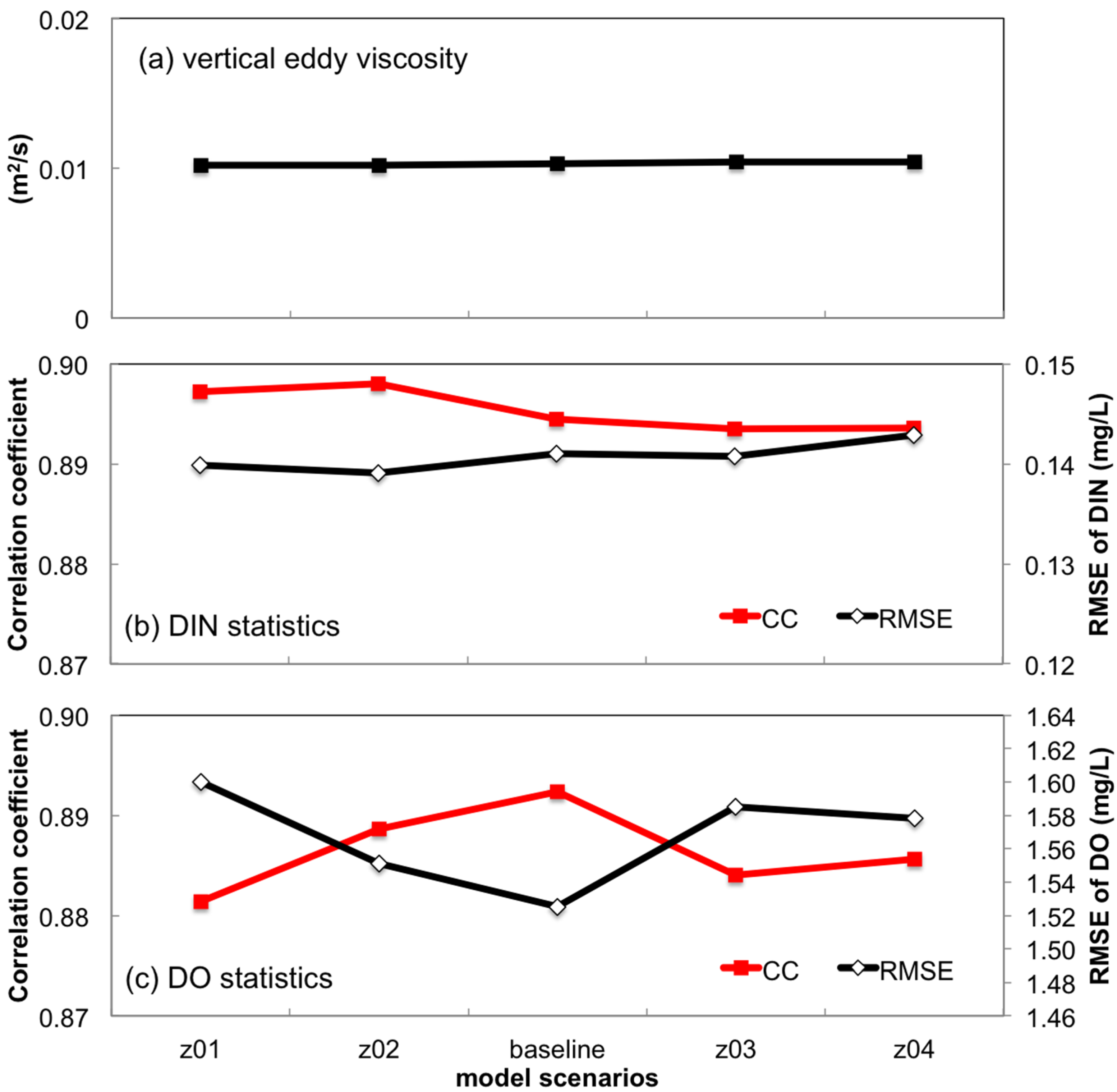
3.2.3. Sensitivity to Bottom Roughness Length Scale

Another uncertainty originating from the hydrodynamic simulation was the bottom stress, and the input of the spatially-non-uniform bottom roughness length scale regulated the drag coefficient and the bottom friction. Compared to the calibrated model [31], the bottom roughness length scale was scaled to 25%, 50%, 200% and 300% to investigate its impacts on nutrient transport and DO variation (Table 2).
Along the gradient of bottom roughness, the vertical eddy viscosity did not vary much among these scenarios (Figure 11a). Moreover, the differences in CCs and RMSEs of DIN in these five scenarios were below 0.005 and 0.004 (mg/L), respectively (Figure 11b). The minimal variation among the nitrogen simulation from these scenarios indicated that bottom roughness was hardly a main uncertainty source for nitrogen simulation. In contrast, the discrepancy in DO simulation was slightly larger than that in DIN, and the range of differences in CCs and RMSEs among cases could exceed 0.01 and 0.07 (mg/L), respectively (Figure 11c). This phenomenon was likely related to the horizontal oxygen exchange near the bottom since the vertical mixing was not prominently affected (Figure 11a). The baseline case achieved the highest correlation with the DO observation and the lowest error, even though it did not perform the best in DIN simulation (Figure 11b,c). Based on the model skills of DIN and DO, the two variables responded relatively strongly to bottom roughness compared with the others.

3.3. Uncertainties Associated with the Model Inputs

3.3.1. Sensitivity to Boundary Nutrient Loading

Boundary nutrient loading has been rated as an important driver in water quality models, and the accuracy of nutrient loading from riverine, benthic and other sources in a water quality model is fundamental to guide and advise the nutrient reduction plan [28]. It is essential to test how the variations in nutrient loading act on the water quality modeling results in the modeling framework. As many previous studies concentrated on the effect of nutrient loading on hypoxia in CB [3,4], we placed an emphasis on the response of phytoplankton production to complement previous studies.
The riverine nitrogen, phosphorus and silicon loading were scaled at the same time by 25%, 50%, 75%, 80%, 90%, 95%, 105%, 110% and 120% in order to maintain the stoichiometry in nutrient sources (Table 2), and the freshwater discharge was not adjusted to avoid changes in the physical environment (e.g., stratification field). We examined the surface DIN concentration and phytoplankton biomass in May, the period of peak spring bloom in 2010. With nutrient enrichment, the surface DIN concentration and phytoplankton biomass displayed a near linear increase (Figure 12). Based on our estimation, the 5%, 10% and 20% variation in nutrient loading could result in 2.9%–3.4%, 5.9%–6.8% and 11.2%–14.0% fluctuation in inner-bay nutrient concentration and phytoplankton biomass. In comparison, the benthic nutrient loading from the sediment diagenesis sub-model had a less significant control on the nutrient concentration and phytoplankton biomass in the water column, since up to 20% variation in benthic nutrient inputs could cause only 2.4%–2.9% alteration in surface DIN concentration and 4.2%–5.0% changes in surface phytoplankton biomass (Figure 12). Our model responded insensitively to the nutrient concentration at the open boundary, where nutrients and phytoplankton are flushed out of the model domain (Figure 1), since up to a 100% alteration in open boundary nutrient concentration led to a negligible (0.7%–0.9%) decrease of inner-bay nutrient concentration and phytoplankton biomass (Figure 12).
Therefore, the riverine nutrient loading or nutrients from the watershed accounted for the largest uncertainty in the water quality simulation among all of the loading sources. The little contribution of open boundary loading was probably due to the low nutrient concentration on the continental shelf compared to in the estuary [52]. These results are similar to those in the CBEMP [53]. Thus, the loading estimation in the watershed model was critical to the biogeochemical simulation in the estuary, and the anthropogenic nutrient reduction in the CB watershed is the most effective way of alleviating eutrophication in the water column.

3.3.2. Sensitivity of Predation Terms to Phytoplankton Simulation

There are two major predation sources of phytoplankton in the model, zooplankton and suspension feeders (e.g., Corbicula fluminea, Rangia cuneata and Crassostrea virginica). We switched off these two modules to examine their controls on the phytoplankton biomass. When the zooplankton predation was eliminated, the surface phytoplankton biomass in May increased by 3.8%. When we turned off the filtration on the benthos, the surface phytoplankton biomass in May increased by 1.6%. That is, zooplankton predation on phytoplankton was more significant than suspension feeding; however, neither of them could result in a large (>5%) biomass loss during the peak spring bloom in CB, and their sensitivity was not as high as the nutrient loading. Extensive observation of the suspension feeder density and zooplankton spatial distribution is still necessary because they could exert a large influence on the spatial heterogeneity of algal distribution [45].

4. Model Calibration and Validation

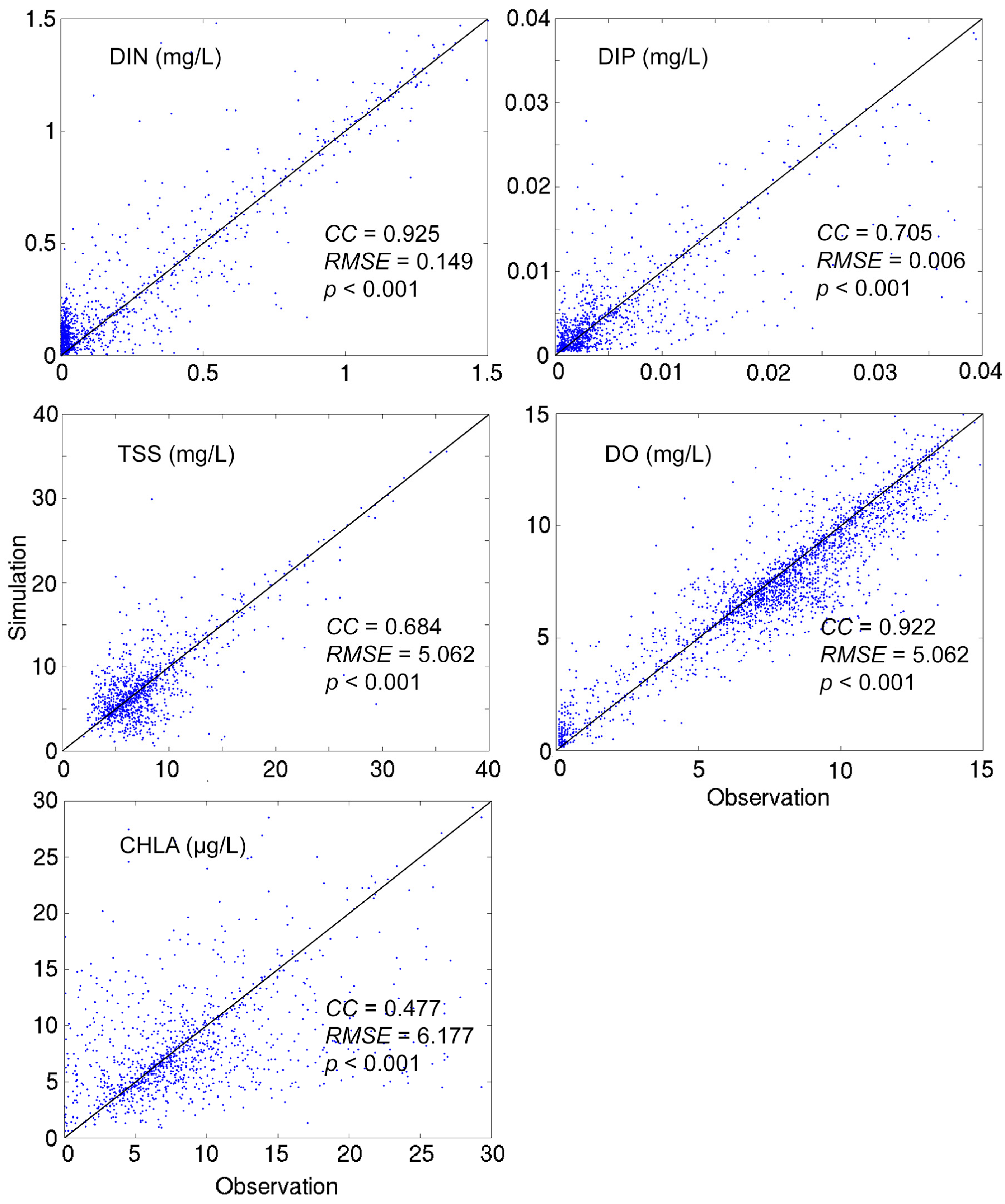
4.1. A 10-Year (2003–2012) Model Simulation

To further validate the model settings, we ran the model in a 10-year (2003–2012) period and evaluated the overall model performance using the CBP mooring data. During this period, modeled DIN, DIP, DO, TSS and CHLA showed significant correlations with observational data (p < 0.001), and their RMSEs were relatively small (Figure 13). Robson [54] reviewed that most reliable aquatic water quality models could simulate nutrients and phytoplankton with CC of 0.632–0.775 and relative error of ~40%. In comparison, our model showed even higher agreement of DIN (CC = 0.925) and DO (CC = 0.922) with empirical data than the above criteria, while the correlations with observed DIP (CC = 0.705) and TSS (CC = 0.684) were within the average range of typical water quality models (Figure 13). However, the CHLA (CC = 0.477) simulated by our model tended to overestimate in low-production periods and was below the criteria (Figure 13).
The desirable modeling confidence of DO and CHLA, two principal water quality criteria for CB [28,55], for the purpose of water quality management was primarily as follows: CC, 0.707 for DO and 0.447 for CHLA; standard deviation, 50% for DO and 300% for CHLA [56]. The RMSEs of both DO and CHLA in our model, whose values were close to the corresponding standard deviation, were less than these criteria; the corresponding correlation coefficients of DO and CHLA also exceeded those in the criteria (Figure 13). Therefore, this modeling package generated reasonably well the representation of the main water quality variables in the 10-year simulation, and the model skill ensured the confidence in utilizing this model in assisting water quality management and studying the complex biophysical interactions driving the CB biogeochemical cycles.
In terms of model calibration to the empirical data, another noteworthy fact is that this modeling system exhibited the best performance in surface CHLA and the second best in bottom CHLA among the five current complex eutrophication models for CB [23], although the simulation skill of CHLA was not as good as other simulated variables in our model (Figure 13). In order to further corroborate the spatial CHLA distribution and figure out the challenges underlying in modeling phytoplankton, we then compared our simulated surface CHLA to that measured by remote sensing in the following subsection.

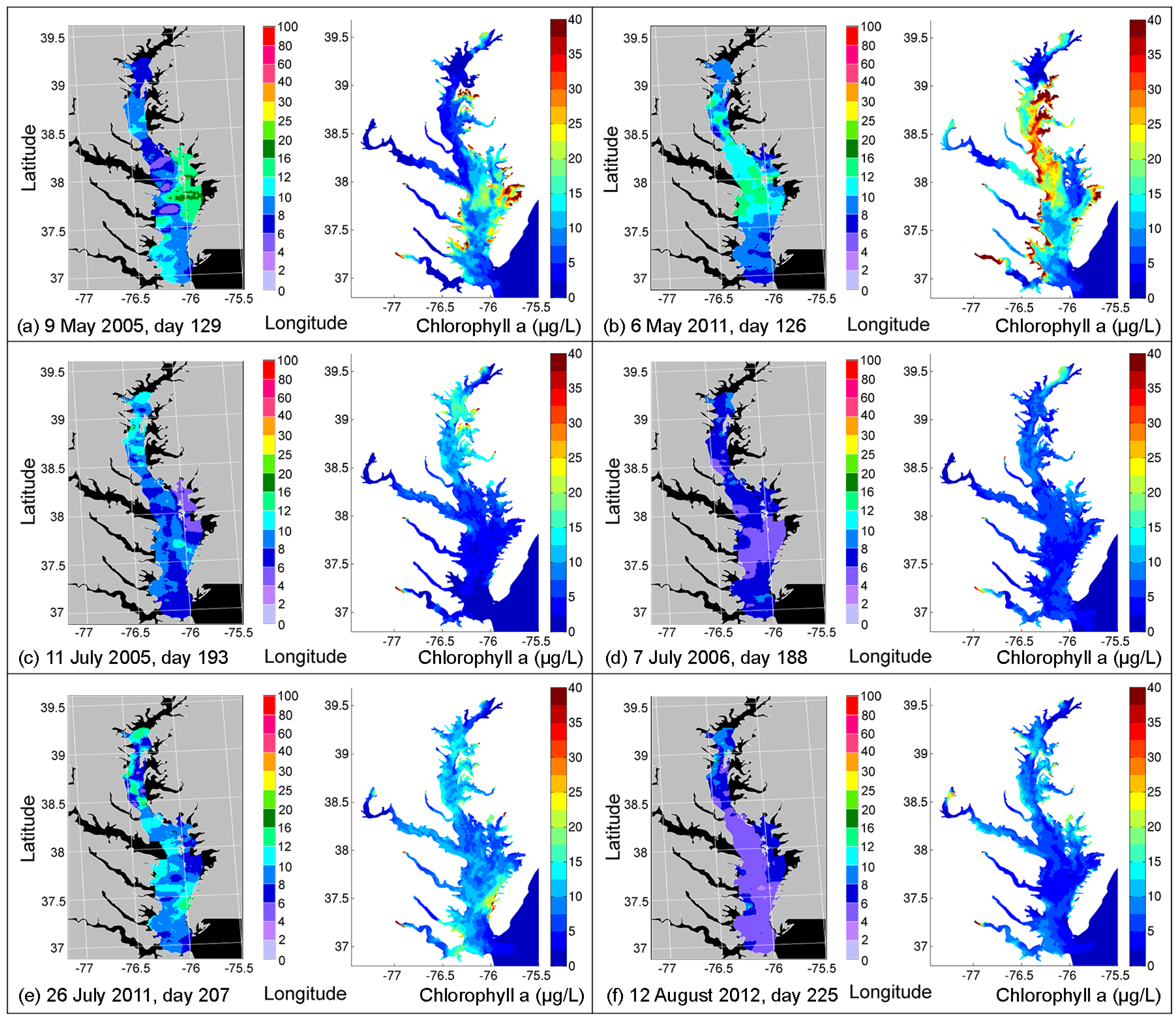
4.2. Comparison of Simulated CHLA with Remote Sensing Images

During the spring bloom (usually peaking in May), the lower-bay and mid-bay areas in both modeled and remote sensing images were characterized by a high CHLA concentration (Figure 14a,b), in which diatoms dominated [6]. In a wet year (e.g., 2011), the magnitude and extent of the spring bloom were greater than other years (Figure 14b). In summer, the entire phytoplankton biomass, with dinoflagellates and cyanobacteria the dominant groups [6], became lower than that in spring, and the chlorophyll maxima were generally shifted northwards due to reduced stream flow (Figure 14c) or even disappeared for lack of nutrient input (Figure 14d). These results were consistent with many previous field observations in CB [5,6,10,26,57,58], which suggested that our model followed the general seasonal and inter-annual patterns of phytoplankton distribution.
Except for the major seasonal pattern, phytoplankton usually appeared in patches (Figure 14a,e,f). These “hot spots” of chlorophyll generally included the eastern embayment (Figure 14a,f), littoral zones (Figure 14e), areas near the Patapsco River (Figure 1 and Figure 14f) and specific mid-bay regions (Figure 14e). Spatial heterogeneity of phytoplankton, probably regulated by the regional nutrient enrichment, grazing, advection, stratification and the balance of various biophysical mechanisms, was a phenomenon frequently observed, but far from well understood [45,59,60]. Our model was capable of capturing most of the realistic CHLA patches, but might slightly deviate in location, extent or magnitude (Figure 14), which partially accounted for the low model skills of CHLA relative to other variables.
The difficulty in accurately simulating the localized and sporadic phytoplankton bloom was one major source of error in CHLA simulation, and it was also noticed in other models [45]. One possible explanation for the inaccuracy in primary production simulation was that phytoplankton growth, an unsteady state, accumulated the errors from processes, such as hydrodynamic conditions, nutrient transport, light attenuation, interspecific competition and predator-prey interaction [60]. Pertaining to our modeling effort, the potential improvement in CHLA simulation desired both field observation and model development from at least the following aspects: investigating vertical migration of phytoplankton, formulating the heterotrophic capability of dinoflagellates, considering sufficient phytoplankton groups and quantifying the grazing pressure by herbivores besides zooplankton.

5. Conclusions

A three-dimensional unstructured grid biophysical model (FVCOM-ICM) was applied to CB and its adjacent coastal ocean to investigate the biophysical controls on the main water quality variables. In the process of model calibration, a series of sensitivity experiments was conducted on major sources of uncertainties. The model showed reasonable agreement with observed water quality variables, such as DIN, DIP, TSS, DO and CHLA during a 10-year simulation period (2003–2012), and the simulated surface CHLA could represent the seasonal and spatial distribution patterns revealed by remote sensing images. The main conclusions based on the sensitivity tests are summarized below.
(1)
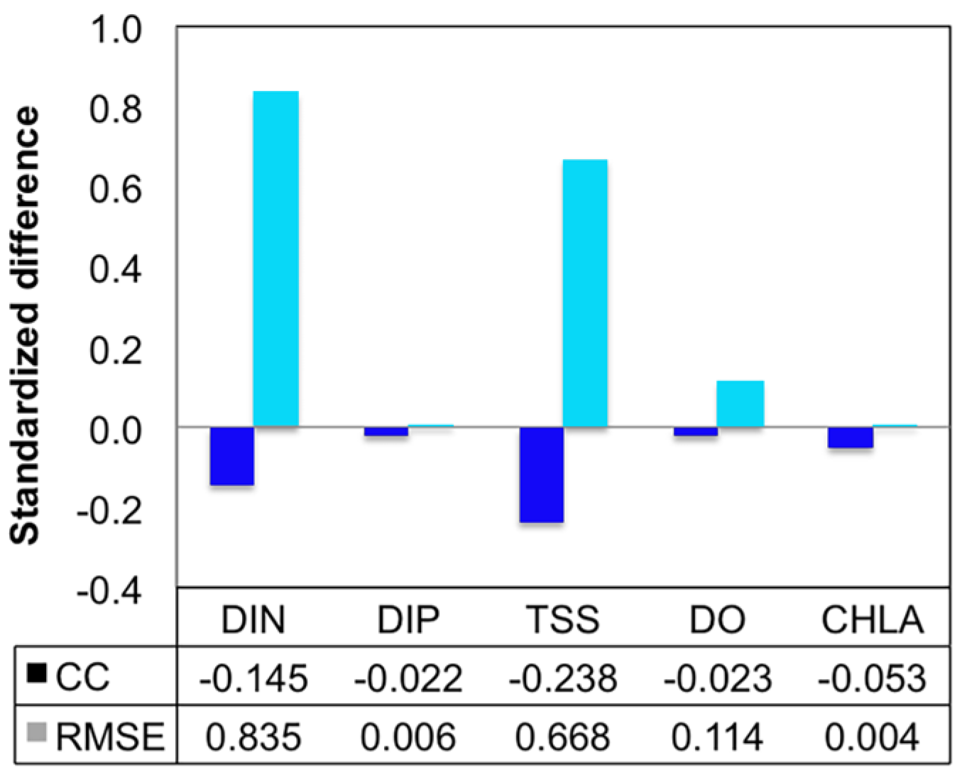
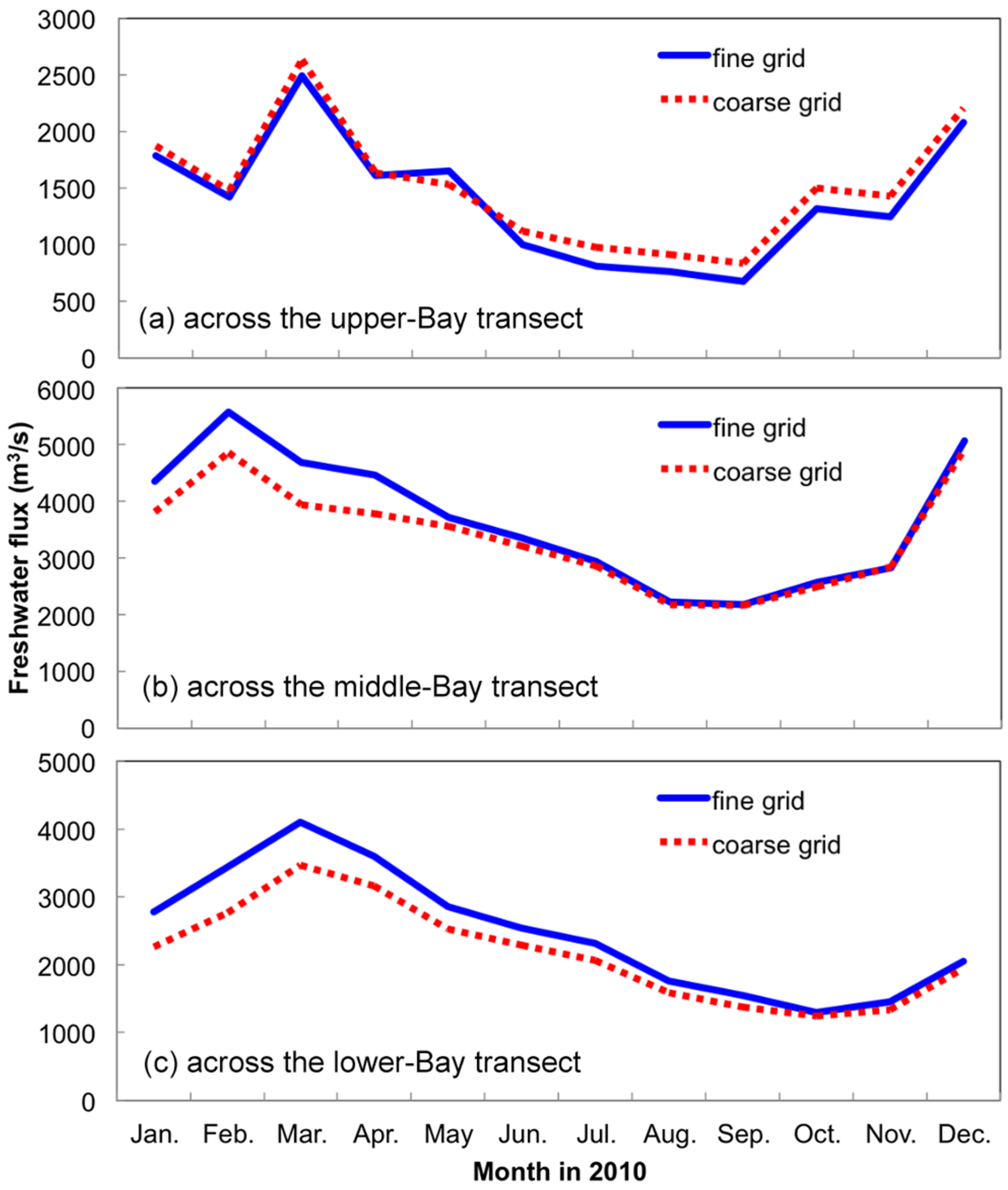
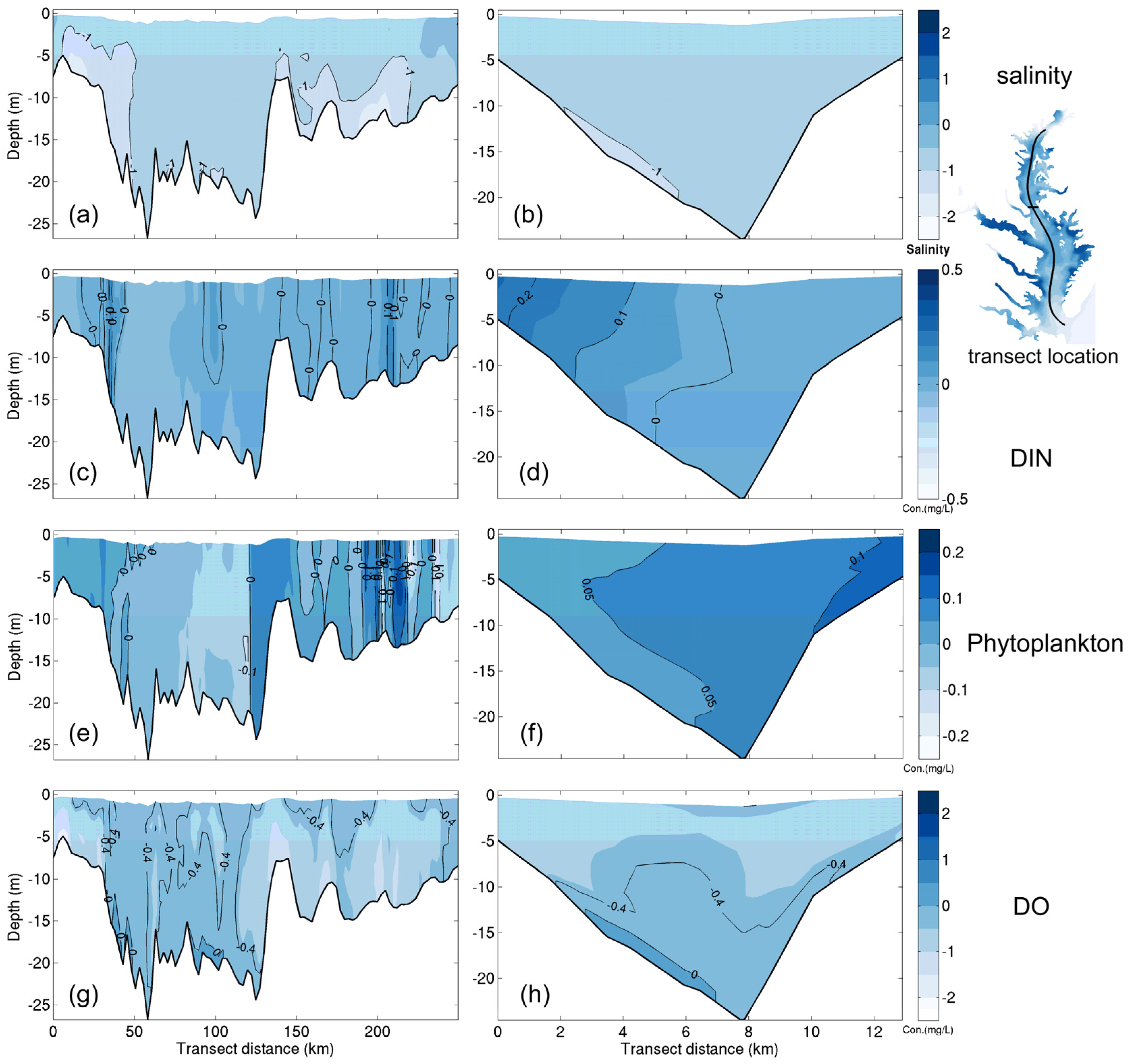
Grid refinement improved the model performance of most variables, particularly for DIN and TSS. The finer grid favored modeling the realistic material transport from the Susquehanna River to the bay mouth, especially in the mid-bay portion. Eleven sigma levels were applied in consideration of the balance between computational accuracy and efficiency. The unstructured grid-based water quality models made it feasible to reach high resolution in biologically-active regions (e.g., littoral zones and the main channel) without significantly adding to the overall computational burden.
(2)
The effects of wind source on DO simulation were compared between the NARR modeled and observed winds. Both winds represented directional asymmetry in summer (southerly winds strongest and westerly weakest), while the observed winds showed lower frequency in southerly winds. The DO simulation forced by these two wind sources had good agreement with empirical data, except that the surface DO was overestimated under the observed winds. Due to stronger mixing from the more frequent southerly winds, the NARR winds were preferred in our water quality model.
(3)
Turbulent mixing and bottom stress were two potential sources of uncertainties in water quality simulation. Appropriate representation of vertical eddy viscosity was propitious to model the vertical oxygen ventilation and the new primary production fueled with recycled nutrients. Bottom friction exerted a moderate impact only on the horizontal oxygen mixing. In terms of water quality simulation, the vertical mixing process was more influential than bottom roughness.
(4)
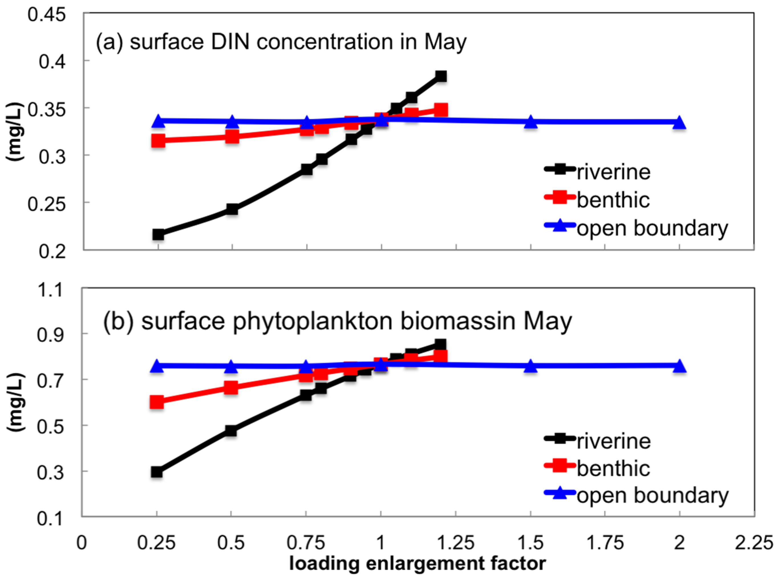
Uncertainties in the riverine source could exert a relatively larger influence on the inner-bay nutrient concentration and phytoplankton biomass during the spring bloom than those in benthic nutrient flux and open boundary loading. Zooplankton predation on phytoplankton was more significant than that of the filtration of suspension feeders.
As a simplification of the real-world systems, all water quality models rely on assumptions and have limitations, including ours. For instance, in addition to those mentioned in Section 4.2, we did not consider the tidal marshes surrounding CB. However, our calibration efforts and sensitivity tests have displayed the feasibility and reliability of such a holistic modeling approach in simulating the main environmental indicators in CB and discerning complex internal biophysical interactions on the lower estuarine-coastal food web. Our biophysical approach will be further utilized to decipher the potential response of water quality cycles in the context of climate change and investigate the estuarine-shelf nutrient exchange.

Acknowledgments

This project is partially supported by the Delmarva Land Grant Institution Cooperative Seed Grant Program. L. Jiang was partially supported by a Department Teaching Assistantship.

Author Contributions

Meng Xia put forward the scientific ideas; design the modeling experiments and organizes the manuscript. Long Jiang calibrated the water quality model and ran the numerical experiments under the supervision of Meng Xia. Both authors contributed to the study.

Conflicts of Interest

The authors declare no conflict of interest.

References

  1. Gillmore, J.; Glendening, P.; Ridge, T.; Williams, A.; Browner, C.; Bolling, B. Chesapeake 2000 Agreement; United States Environmental Protection Agency Chesapeake Bay Program: Annapolis, MD, USA, 2000. [Google Scholar]
  2. Kemp, W.M.; Boynton, W.R.; Adolf, J.E.; Boesch, D.F.; Boicourt, W.C.; Brush, G.; Cornwell, J.C.; Fisher, T.R.; Glibert, P.M.; Hagy, J.D.; et al. Eutrophication of Chesapeake Bay: Historical trends and ecological interactions. Mar. Ecol. Prog. Ser. 2005, 303, 1–29. [Google Scholar] [CrossRef]
  3. Hagy, J.D.; Boynton, W.R.; Keefe, C.W.; Wood, K.V. Hypoxia in Chesapeake Bay, 1950–2001: Long-term change in relation to nutrient loading and river flow. Estuaries 2004, 27, 634–658. [Google Scholar] [CrossRef]
  4. Murphy, R.R.; Kemp, W.M.; Ball, W.P. Long-term trends in Chesapeake Bay seasonal hypoxia, stratification, and nutrient loading. Estuar. Coasts 2011, 34, 1293–1309. [Google Scholar] [CrossRef]
  5. Harding, L.W.; Mallonee, M.E.; Perry, E.S. Toward a predictive understanding of primary productivity in a temperate, partially stratified estuary. Estuar. Coast. Shelf Sci. 2002, 55, 437–463. [Google Scholar] [CrossRef]
  6. Marshall, H.G.; Lane, M.F.; Nesius, K.K.; Burchardt, L. Assessment and significance of phytoplankton species composition within Chesapeake Bay and Virginia tributaries through a long-term monitoring program. Environ. Monit. Assess. 2009, 150, 143–155. [Google Scholar] [CrossRef] [PubMed]
  7. Smith, E.M.; Kemp, W.M. Seasonal and regional variations in plankton community production and respiration for Chesapeake Bay. Mar. Ecol. Prog. Ser. 1995, 116, 217–231. [Google Scholar] [CrossRef]
  8. Harding, L.W. Long-term trends in the distribution of phytoplankton in Chesapeake Bay: Roles of light, nutrients and streamflow. Mar. Ecol. Prog. Ser. 1994, 104, 267. [Google Scholar] [CrossRef]
  9. Prasad, M.B.K.; Sapiano, M.R.; Anderson, C.R.; Long, W.; Murtugudde, R. Long-term variability of nutrients and chlorophyll in the Chesapeake Bay: A retrospective analysis, 1985–2008. Estuar. Coasts 2010, 33, 1128–1143. [Google Scholar] [CrossRef]
  10. Son, S.; Wang, M.; Harding, L.W. Satellite-measured net primary production in the Chesapeake Bay. Remote Sens. Environ. 2014, 144, 109–119. [Google Scholar] [CrossRef]
  11. Cerco, C.F.; Kim, C.-S.; Noel, M.R. The 2010 Chesapeake Bay Eutrophication Model; U.S. Army Corps of Engineers Waterways Experiment Station: Vicksburg, MS, USA, 2010. [Google Scholar]
  12. Feng, Y.; Friedrichs, M.A.; Wilkin, J.; Tian, H.; Yang, Q.; Hofmann, E.E.; Wiggert, J.D.; Hood, R.R. Chesapeake Bay nitrogen fluxes derived from a land-estuarine ocean biogeochemical modeling system: Model description, evaluation and nitrogen budgets. J. Geophys. Res. Biogeosci. 2015, 120, 1666–1695. [Google Scholar] [CrossRef]
  13. Pennock, J.R. Chlorophyll distributions in the Delaware estuary: Regulation by light-limitation. Estuar. Coast. Shelf Sci. 1985, 21, 711–725. [Google Scholar] [CrossRef]
  14. Jiang, L.; Xia, M.; Ludsin, S.A.; Rutherford, E.S.; Mason, D.M.; Jarrin, J.M.; Pangle, K.L. Biophysical modeling assessment of the drivers for plankton dynamics in dreissenid-colonized western Lake Erie. Ecol. Model. 2015, 308, 18–33. [Google Scholar] [CrossRef]
  15. Testa, J.M.; Li, Y.; Lee, Y.J.; Li, M.; Brady, D.C.; di Toro, D.M.; Kemp, W.M.; Fitzpatrick, J.J. Quantifying the effects of nutrient loading on dissolved O2 cycling and hypoxia in Chesapeake Bay using a coupled hydrodynamic-biogeochemical model. J. Mar. Syst. 2014, 139, 139–158. [Google Scholar] [CrossRef]
  16. Xia, M.; Craig, P.M.; Schaeffer, B.; Stoddard, A.; Liu, Z.; Peng, M.; Zhang, H.; Wallen, C.M.; Bailey, N.; Mandrup-Poulsen, J. Influence of physical forcing on bottom-water dissolved oxygen within Caloosahatchee River Estuary, Florida. J. Environ. Eng. 2010, 136, 1032–1044. [Google Scholar] [CrossRef]
  17. Xia, M.; Craig, P.M.; Wallen, C.M.; Stoddard, A.; Mandrup-Poulsen, J.; Peng, M.; Schaeffer, B.; Liu, Z. Numerical simulation of salinity and dissolved oxygen at Perdido Bay and adjacent coastal ocean. J. Coast. Res. 2011, 27, 73–86. [Google Scholar] [CrossRef]
  18. Xia, M.; Jiang, L. Influence of wind and river discharge on the hypoxia in a shallow bay. Ocean Dyn. 2015, 65, 665–678. [Google Scholar] [CrossRef]
  19. Fitzpatrick, J.J. Assessing skill of estuarine and coastal eutrophication models for water quality managers. J. Mar. Syst. 2009, 76, 195–211. [Google Scholar] [CrossRef]
  20. Ganju, N.K.; Brush, M.J.; Rashleigh, B.; Aretxabaleta, A.L.; del Barrio, P.; Grear, J.S.; Harris, L.A.; Lake, S.J.; McCardell, G.; O’Donnell, J.; et al. Progress and challenges in coupled hydrodynamic-ecological estuarine modeling. Estuar. Coasts 2015, 39, 311–332. [Google Scholar] [CrossRef]
  21. Khangaonkar, T.; Sackmann, B.; Long, W.; Mohamedali, T.; Roberts, M. Simulation of annual biogeochemical cycles of nutrient balance, phytoplankton bloom(s), and DO in Puget Sound using an unstructured grid model. Ocean Dyn. 2012, 62, 1353–1379. [Google Scholar] [CrossRef]
  22. Ganju, N.K.; Sherwood, C.R. Effect of roughness formulation on the performance of a coupled wave, hydrodynamic, and sediment transport model. Ocean Model. 2010, 33, 299–313. [Google Scholar] [CrossRef]
  23. Irby, I.D.; Friedrichs, M.A.M.; Friedrichs, C.T.; Bever, A.J.; Hood, R.R.; Lanerolle, L.W.J.; Scully, M.E.; Sellner, K.; Shen, J.; Testa, J.; et al. Challenges associated with modeling low-oxygen waters in Chesapeake Bay: A multiple model comparison. Biogeosciences 2016, 13, 2011–2028. [Google Scholar] [CrossRef]
  24. Kim, T.; Khangaonkar, T. An offline unstructured biogeochemical model (UBM) for complex estuarine and coastal environments. Environ. Model. Softw. 2012, 31, 47–63. [Google Scholar] [CrossRef]
  25. Shen, J.; Wang, H.V. Determining the age of water and long-term transport timescale of the Chesapeake Bay. Estuar. Coast. Shelf Sci. 2007, 74, 585–598. [Google Scholar] [CrossRef]
  26. Fisher, T.R.; Harding, L.W.; Stanley, D.W.; Ward, L.G. Phytoplankton, nutrients, and turbidity in the Chesapeake, Delaware, and Hudson estuaries. Estuar. Coast. Shelf Sci. 1988, 27, 61–93. [Google Scholar] [CrossRef]
  27. Wang, D.-P. Wind-driven circulation in the Chesapeake Bay, winter 1975. J. Phys. Oceanogr. 1979, 9, 564–572. [Google Scholar] [CrossRef]
  28. U.S. Environmental Protection Agency. Chesapeake Bay Total Maximum Daily Load for Nitrogen, Phosphorus, and Sediment; Chesapeake Bay Program Office: Annapolis, MD, USA, 2010.
  29. Testa, J.M.; Kemp, W.M. Hypoxia-induced shifts in nitrogen and phosphorus cycling in Chesapeake Bay. Limnol. Oceanogr. 2012, 57, 835–850. [Google Scholar] [CrossRef]
  30. Li, J.; Glibert, P.M.; Gao, Y. Temporal and spatial changes in Chesapeake Bay water quality and relationships to Prorocentrum minimum, Karlodinium veneficum, and CyanoHAB events, 1991–2008. Harmful Algae 2015, 42, 1–14. [Google Scholar] [CrossRef]
  31. Jiang, L.; Xia, M. Dynamics of the Chesapeake Bay outflow plume: Realistic plume simulation and its seasonal and interannual variability. J. Geophys. Res. Oceans 2016, 121, 1424–1445. [Google Scholar] [CrossRef]
  32. Di Toro, D.M.; Fitzpatrick, J.J. Chesapeake Bay Sediment Flux Model; HydroQual, Inc.: Mahwah, NJ, USA, 1993. [Google Scholar]
  33. Meyers, M.B.; di Toro, D.M.; Lowe, S.A. Coupling suspension feeders to the Chesapeake Bay Eutrophication Model. Water Qual. Ecosyst. Model. 2000, 1, 123–140. [Google Scholar] [CrossRef]
  34. Cerco, C.F.; Cole, T. User’s Guide to the CE-QUAL-ICM Three-Dimensional Eutrophication Model: Release, version 1.0 Report; US Army Engineer Waterways Experiment Station: Vicksburg, MS, USA, 1995. [Google Scholar]
  35. Malone, T.C.; Crocker, L.H.; Pike, S.E.; Wendler, B.W. Influences of river flow on the dynamics of phytoplankton production in a partially stratified estuary. Mar. Ecol. Prog. Ser. 1988, 48, 235–249. [Google Scholar] [CrossRef]
  36. U.S. Environmental Protection Agency. Chesapeake Bay Program water quality data. Available online: http://www.chesapeakebay.net/data (accessed on 18 August 2016).
  37. National Atmospheric Deposition Program data. Available online: http://nadp.sws.uiuc.edu/data/ (accessed on 18 August 2016).
  38. World Ocean Atlas 2005 data. Available online: http://www.nodc.noaa.gov/OC5/WOA05/pr_woa05.html (accessed on 18 August 2016).
  39. National Center for Environmental Prediction. North America Regional Reanalysis data. Available online: http://www.esrl.noaa.gov/psd/data/gridded/data.narr.html (accessed on 18 August 2016).
  40. Chesapeake Bay Remote Sensing Program data. Available online: http://www.cbrsp.org/index.html (accessed on 18 August 2016).
  41. U.S. Geological Survey data. Available online: http://md.water.usgs.gov/waterdata/chesinflow/wy/ (accessed on 18 August 2016).
  42. National Data Buoy Center data. Available online: http://www.ndbc.noaa.gov (accessed on 18 August 2016).
  43. National Centers for Environmental Information data. Available online: http://www.ncdc.noaa.gov (accessed on 18 August 2016).
  44. Boynton, W.R.; Garber, J.H.; Summers, R.; Kemp, W.M. Inputs, transformations, and transport of nitrogen and phosphorus in Chesapeake Bay and selected tributaries. Estuaries 1995, 18, 285–314. [Google Scholar] [CrossRef]
  45. Cerco, C.F.; Noel, M.R. Incremental improvements in Chesapeake Bay environmental model package. J. Environ. Eng. 2005, 131, 745–754. [Google Scholar] [CrossRef]
  46. Chenillat, F.; Franks, P.J.; Rivière, P.; Capet, X.; Grima, N.; Blanke, B. Plankton dynamics in a cyclonic eddy in the Southern California Current System. J. Geophys. Res. Oceans 2015, 120, 5566–5588. [Google Scholar] [CrossRef]
  47. Du, J.; Shen, J. Decoupling the influence of biological and physical processes on the dissolved oxygen in the Chesapeake Bay. J. Geophys. Res. Oceans 2015, 120, 78–93. [Google Scholar] [CrossRef]
  48. Scully, M.E. Physical controls on hypoxia in Chesapeake Bay: A numerical modeling study. J. Geophys. Res. Oceans 2013, 118, 1239–1256. [Google Scholar] [CrossRef]
  49. Scully, M.E. Wind modulation of dissolved oxygen in Chesapeake Bay. Estuar. Coasts 2010, 33, 1164–1175. [Google Scholar] [CrossRef]
  50. Belyaev, V.I. Modelling the influence of turbulence on phytoplankton photosynthesis. Ecol. Model. 1992, 60, 11–29. [Google Scholar] [CrossRef]
  51. Estrada, M.; Berdalet, E. Phytoplankton in a turbulent world. Sci. Mar. 1998, 61 (Suppl. 1), 125–140. [Google Scholar]
  52. Filippino, K.C.; Bernhardt, P.W.; Mulholland, M.R. Chesapeake Bay plume morphology and the effects on nutrient dynamics and primary productivity in the coastal zone. Estuar. Coasts 2009, 32, 410–424. [Google Scholar] [CrossRef]
  53. Cerco, C.F.; Noel, M.R. The 2002 Chesapeake Bay Eutrophication Model; U.S. Army Corps of Engineers, Waterways Experiment Station: Vicksburg, MS, USA, 2004. [Google Scholar]
  54. Robson, B.J. State of the art in modelling of phosphorus in aquatic systems: Review, criticisms and commentary. Environ. Model. Softw. 2014, 61, 339–359. [Google Scholar] [CrossRef]
  55. Harding, L.W.; Batiuk, R.A.; Fisher, T.R.; Gallegos, C.L.; Malone, T.C.; Miller, W.D.; Mulholland, M.R.; Paerl, H.W.; Perry, E.S.; Tango, P. Scientific bases for numerical chlorophyll criteria in Chesapeake Bay. Estuar. Coasts 2014, 37, 134–148. [Google Scholar] [CrossRef]
  56. Linker, L.C.; Shenk, G.W.; Wang, P.; Cerco, C.F.; Butt, A.J.; Tango, P.J.; Savidge, R.W. A Comparison of the Chesapeake Bay Estuary Model Calibration with 1985–1994 Observed Data and Method of Application to Water Quality Criteria; Modeling Subcommittee of the Chesapeake Bay Program: Annapolis, MD, USA, 2002. [Google Scholar]
  57. Adolf, J.E.; Yeager, C.L.; Miller, W.D.; Mallonee, M.E.; Harding, L.W. Environmental forcing of phytoplankton floral composition, biomass, and primary productivity in Chesapeake Bay, USA. Estuar. Coast. Shelf Sci. 2006, 67, 108–122. [Google Scholar] [CrossRef]
  58. Harding, L.W.; Meeson, B.W.; Fisher, T.R. Phytoplankton production in two east coast estuaries: Photosynthesis-light functions and patterns of carbon assimilation in Chesapeake and Delaware Bays. Estuar. Coast. Shelf Sci. 1986, 23, 773–806. [Google Scholar] [CrossRef]
  59. Bronk, D.A.; Glibert, P.M.; Malone, T.C.; Banahan, S.; Sahlsten, E. Inorganic and organic nitrogen cycling in Chesapeake Bay: Autotrophic versus heterotrophic processes and relationships to carbon flux. Aquat. Microb. Ecol. 1998, 15, 177–189. [Google Scholar] [CrossRef]
  60. Roman, M.; Zhang, X.; McGilliard, C.; Boicourt, W. Seasonal and annual variability in the spatial patterns of plankton biomass in Chesapeake Bay. Limnol. Oceanogr. 2005, 50, 480–492. [Google Scholar] [CrossRef]
Figure 1. Model grid and bathymetry of Chesapeake Bay (CB) and its adjacent coastal ocean with river nodes, data sites and three transects. The bottom right panels are the zoom-in of the boxed area from two sets of grids generated for sensitivity experiments on spatial resolution. Sus, Susquehanna River; Ptp, Patapsco River; Che, Chester River; Pat, Patuxent River; Cho, Choptank River; Pot, Potomac River; Nan, Nanticoke River; Rap, Rappahannock River; Yor, York River; Jam, James River.
Jmse 04 00052 g001
Figure 2. Schematic flow diagram of ICM set up for Chesapeake Bay. LDOC, RDOC, LPOC, RPOC, labile/refractory dissolved/particulate organic carbon; LDON, RDON, LPON, RPON, labile/refractory dissolved/particulate organic nitrogen; LDOP, RDOP, LPOP, RPOP, labile/refractory dissolved/particulate organic phosphorus; PSi/DSi, particulate/dissolved silica; COD, chemical oxygen demand; DO, dissolved oxygen; NO23, nitrite and nitrate; NH4, ammonia; PO4, phosphate; DIN, dissolved inorganic nitrogen.
Jmse 04 00052 g002
Figure 3. Time series of observed (open dots) and simulated (black solid line, fine-grid results; red dash line, coarse-grid results) water quality and phytoplankton state variables at three sampling sites in Chesapeake Bay (Figure 1) in 2010: NH4 (ammonia), NO23 (nitrite and nitrate), PO4 (phosphate), TSS (total suspended solids), DO (dissolved oxygen) and CHLA (chlorophyll-a).
Jmse 04 00052 g003
Figure 4. Standardized difference of CC and RMSE in the coarse-grid model compared to the fine-grid model. Standardized score are calculated as follows: ZCC = (CCcoarseCCfine)/CCfine, ZRMSE = (RMSEcoasrseRMSEfine)/RMSEfine. CC and RMSE denote the correlation coefficient and root mean squared error between the model simulation and the observation, respectively. The raw data of CC and RMSE are shown in Table 3. The five variables are DIN (dissolved inorganic nitrogen, including ammonia, nitrite and nitrate), DIP (dissolved inorganic phosphorus), TSS (total suspended solids), DO (dissolved oxygen) and CHLA (chlorophyll-a).
Jmse 04 00052 g004
Figure 5. Freshwater transport across the (a) upper-, (b) middle-, and (c) lower-Bay transects (Figure 1) in the fine-gird (blue solid line) and coarse-grid (red dash line) models.
Jmse 04 00052 g005
Figure 6. Time series of observed (open dots) and simulated (black solid line, results of 11 sigma levels; black dash line, results of six (a,b) or 21 (c,d) sigma levels) phosphate (a,c) and CHLA (b,d) at Station CB4.3C in Chesapeake Bay (Figure 1) in 2010.
Jmse 04 00052 g006
Figure 7. Difference in simulated (a) along-bay and (b) across-bay salinity in May; (c) along-bay and (d) across-bay dissolved inorganic nitrogen in May; (e) along-bay and (f) across-bay phytoplankton biomass in May and (g) along-bay and (h) across-bay dissolved oxygen in July between the 11-sigma-level and 21-sigma-level models. The along-bay and across-bay transects are shown on the rightmost panel.
Jmse 04 00052 g007
Figure 8. Wind rose plot in the hypoxia season (from May–August) in 2010: (a) spatially-averaged NARR data; and (b) observation from National Data Buoy Center and National Centers for Environmental Information.
Jmse 04 00052 g008
Figure 9. Time series of observed (open dots) and simulated (black solid line, results driven by the NARR wind data; black dashed line, results driven by the observed wind data (Table 2); blue dashed line, results using NARR wind-driven mixing and observed wind-driven reaeration) dissolved oxygen at two sampling sites in Chesapeake Bay (Figure 1) in 2010: Station CB2.2 at (a) the surface and (b) the bottom; Station CB4.3C at (a) the surface and (b) the bottom.
Jmse 04 00052 g009
Figure 10. (a) The average eddy viscosity; (b) the surface-to-bottom difference of dissolved oxygen in the hypoxia season (from May–August); (c) surface phytoplankton biomass in summer (from June–August); CC and RMSE of (d) dissolved oxygen and (e) chlorophyll-a in 2010 in the five scenarios of varying eddy viscosity (az1, az2, baseline, az3 and az4 in Table 2). CC and RMSE denote the correlation coefficient and root mean squared error between the model simulation and the observation, respectively.
Jmse 04 00052 g010
Figure 11. (a) The average eddy viscosity; CC and RMSE of (b) dissolved inorganic nitrogen and (c) dissolved oxygen in 2010 in five scenarios of varying bottom roughness length scale (z01, z02, baseline, z03 and z04 in Table 2). CC and RMSE denote the correlation coefficient and root mean squared error between the model simulation and the observation, respectively.
Jmse 04 00052 g011
Figure 12. The relationship between the enlargement factor of riverine, benthic and open boundary nutrient loading (see Table 2) and the (a) surface dissolved inorganic nitrogen concentration and (b) phytoplankton biomass in May 2010.
Jmse 04 00052 g012
Figure 13. Comparison between modeled and observed dissolved inorganic nitrogen (DIN) and phosphorus (DIP), dissolved oxygen (DO), total suspended solids (TSS) and chlorophyll-a (CHLA) from 2003–2012. CC and p denote the correlation coefficient and its p-value, and RMSE is the root mean squared error.
Jmse 04 00052 g013
Figure 14. Remote sensing and simulated surface chlorophyll-a of Chesapeake Bay on: (a) 9 May 2005; (b) 6 May 2011; (c) 11 July 2005; (d) 7 July 2006; (e) 26 July 2011; and (f) 12 August 2012. Remote sensing data source: Chesapeake Bay Remote Sensing Program.
Jmse 04 00052 g014
Table 1. Key kinetic parameters used for the ICM for Chesapeake Bay. CHLA, chlorophyll = a.
ParametersValueLiterature Range
Settling velocity W (CYN, m/day)00–0.1 [11,14,34]
Settling velocity W (DIA, m/day)0.20–0.5 [11,14,21,34]
Settling velocity W (DINO, m/day)0.10–0.2 [21,34]
Max photosynthetic rate Pm (CYN, day−1)150100–270 [11,14,34]
Max photosynthetic rate Pm (DIA, day−1)300200–400 [11,14,21,34]
Max photosynthetic rate Pm (DINO, day−1)200200–350 [21,34]
C:CHLA ratio CChl (CYN)5030–143 [11,14,34,35]
C:CHLA ratio CChl (DIA)3730–143 [11,14,21,34,35]
C:CHLA ratio CChl (DINO)5030–143 [21,34,35]
Half-saturation KH-DIN (CYN, mg/L)0.020.01–0.03 [11,14,34]
Half-saturation KH-DIN (DIA, mg/L)0.0250.003–0.923 [11,14,21,34]
Half-saturation KH-DIN (DINO, mg/L)0.0250.003–0.923 [21]
Half-saturation KH-DIP (all, mg/L)0.00250.001–0.195 [11,14,21,34]
Half-saturation KH-DSi (DIA, mg/L)0.030.01–0.05 [11,14,21,34]
Photosynthesis Topt (CYN, °C)2522–30 [11,14,34]
Photosynthesis Topt (DIA, °C)1612–35 [11,14,21,34]
Photosynthesis Topt (DINO, °C)2418–35 [21]
Respiration Tref (°C)2020 [11,34]
Percentage of active respiration Pres0.250.25 [11,14,21,34]
Basal metabolic rate M (CYN, day−1)0.030.03–0.05 [11,14,34]
Basal metabolic rate M (DIA, day−1)0.010.01–0.1 [11,14,21,34]
Basal metabolic rate M (DINO, day−1)0.020.01–0.1 [21,34]
Herbivore predation rate F (CYN, day−1)0.030.01–0.05 [14,34]
Herbivore predation rate F (DIA, day−1)0.10.05–1 [14,21,34]
Herbivore predation rate F (DINO, day−1)0.50.05–1 [21]
Max zooplankton predation ration (SZ, day−1)2.250.8–2.25 [11,14]
Max zooplankton predation ration (LZ, day−1)1.750.8–1.75 [11,14]
Settling velocity of particles (m/day)0.250.03–0.8 [11,14,21,34]
Max nitrification rate (g·m−3·day−1)0.0750.01–0.75 [11,14,21,34]
Optimal nitrification temperature (°C)3025–35 [11,14,21,34]
Table 2. A list of model sensitivity experiments.
ScenariosTreatment
baselineDescribed in Section 2 and [31]
coarseUsing a low-resolution model grid a (Figure 1)
sigma06, sigma20Using 6 and 21 uniform sigma levels; i.e., each sigma layer represents 1/5 and 1/20 of the water depth, respectively
obsUsing wind data from National Data Buoy Center and National Centers for Environmental Information
obs + narrUsing observed wind to drive mixing and NARR wind to drive reaeration
az1, az2, az3, az4Vertical eddy viscosity (az) computed in the hydrodynamic model was roughly 25%, 50%, 200% and 400% of the baseline scenario. The adjustment of vertical eddy viscosity is achieved by altering the Prandtl number
z01, z02, z03, z04The bottom roughness length scale (z0) was 25%, 50%, 200% and 300% of the baseline scenario
r0.25, r0.50, r0.75, r0.80, r0.90, r0.95, r1.05, r1.10, r1.20The riverine nutrient loading was 25%, 50%, 75%, 80%, 90%, 95%, 105%, 110% and 120% of the baseline scenario
bf0.25, bf0.50, bf0.75, bf0.8, bf0.9, bf1.1, bf1.2The benthic nutrient flux was 80%, 90%, 110% and 120% of the baseline scenario
o0.25, o0.50, o0.75, o1.5, o2.0The open boundary nutrient concentration was 25%, 50%, 75%, 150% and 200% of the baseline scenario
nzp and nsfPredation of zooplankton (nzp) and suspension feeder (nsf) on phytoplankton was switched off, respectively
Note: a: the fine and coarse grid is presented in Figure 1 with the average inner-bay grid size of 1.43 km and 1.74 km, respectively.
Table 3. Model observation statistics with two sets of model grids in 2010.
GridVariablenCCpRMSE
FineDIN1050.895<0.0010.141
DIP1050.410<0.0010.016
TSS1050.801<0.0012.209
DO2100.892<0.0011.525
CHLA1040.480<0.0017.516
CoarseDIN1050.765<0.0010.259
DIP1050.400<0.0010.016
TSS1050.610<0.0013.686
DO2100.872<0.0011.700
CHLA1040.455<0.0017.548
Note: n: sample size; CC and p: correlation coefficient and its p-value; RMSE: root mean squared error.

