Structure-Borne Wave Radiation by Impact and Vibratory Piling in Offshore Installations: From Sound Prediction to Auditory Damage ^†

Abstract

Anthropogenic noise emission in the marine environment is a key issue nowadays and has drawn the attention of regulatory bodies in various nations. In particular, the noise generated during the installation of foundation piles for the offshore wind industry is considered to be harmful for aquatic species. A reliable prediction of the underwater noise during the installation of a foundation pile is thus essential for the proper assessment of the ecological impact. In this paper, the structure-borne wave radiation is investigated with the help of a semi-analytical model for two cases. The first case considers a pile that is installed with the help of an impact hammer, whereas the second one deals with a pile that is driven into the seabed with the help of a vibratory device. The spatial distribution and the frequency content of the radiated sound are analyzed, and the differences are highlighted between the two cases. The model is validated with data available in the literature that were collected during several measurement campaigns. Subsequently, the predicted noise levels are converted into an equivalent index that reflects the auditory damage to certain marine species, and a method is presented for the derivation of zones of impact around the pile that are based on the noise predictions by the models and the chosen method of installation. This approach can be used to define critical zones within which a predefined level of auditory damage is to be expected based on a specific installation scenario.

1. Introduction

The installation of foundation piles in the marine environment is common practice in many engineering applications, a vast amount of which is related to the offshore oil and gas industry. In addition, piles are the most widely-used support structure for offshore wind power generators due to their conceptual simplicity and favorable installation speed [1]. Each pile is compiled of several steel tubular cross-sections, which are welded together to form a single piece. The latter can reach a diameter of several meters and a length of tens of meters and need to be driven into the marine sediment; a process that requires the development of special installation equipment. In the majority of the installations nowadays, this is achieved with the use of either hydraulic impact hammers or special vibratory devices [2].

During impact pile driving, the hammer delivers a series of blows to the head of the pile [3], forcing the latter to gradually progress into the sediment. The installation of a single pile requires several thousands of blows depending on the pile dimensions, soil conditions and the input energy of the hammer. When a vibratory hammer is used instead, a cyclic (periodic) force is exerted by the hammer at the pile head [4]. Regardless of the method of installation, noise is radiated into the sea environment and can be detected tens of kilometers away from the construction site [5]. There are numerous studies that actually investigate the impact of pile driving and other anthropogenic noise emissions in the marine species [6,7,8,9]. The response of marine mammals and fish to strong impulsive sounds can range from light behavioral disturbance to strong avoidance of the construction region; in extreme cases, even permanent hearing impairment is possible.

Such high noise levels have naturally drawn the attention of regulatory bodies in various nations. Current anti-noise legislation in the Netherlands prohibits pile driving from the first of July till the end of December of each year in order to avoid disturbance of the breeding season of the harbor porpoise [10]. This legislation is expected to be changed in the near future because it causes considerable delay in the construction of new offshore wind farms in the Dutch exclusive economic zone. In the United Kingdom, an evaluation per project takes place. Measures like seal scarers are used together with a few low energy blows of the impact hammer mainly aiming at intimidating the mammals in the neighborhood of the construction site [11]. The German Federal government, on the contrary, adopts certain sound level criteria. These have been set to 160 dB re1 μPa² s for the sound exposure level (SEL) and to 190 dB re 1 μPa for the sound peak pressure level (SPL), both at a distance of 750 m from the sound source [12]. The choice of the aforementioned levels was based on a series of experiments in a harbor porpoise and account additionally for cumulative effects and intra-species variability [13]. Despite the fact that there is yet no overall consensus about the most appropriate way of quantifying the level of noise that can be harmful for marine species, all of the involved parties recognize that certain measures have to be undertaken in order to protect the marine ecosystem.

Modeling of the underwater noise generated by impact piling has been investigated by many authors during the last decade. In the majority of the publications, the modeling of the pile with the surrounding fluid and soil media is achieved by means of the finite element method [14,15,16,17]. These models are usually restricted to cylindrically-symmetric configurations, while the soil is approximated by an equivalent acoustic fluid in order to reduce the computational demands. Finite element models are usually coupled to acoustic propagation models to predict noise at larger distances [18,19]. Despite the fact that these models provide great flexibility in the modeling of complex structural and acoustic domains, they are usually computationally slow, are restricted to noise predictions in the near-field and require the truncation of the infinite soil-fluid domain by the employment of non-reflecting boundaries [20]. Numerical models that couple the structural domain modeled by finite elements (FE) and the exterior soil-fluid domain modeled by boundary elements (BE) also exist [21]. The latter overcome the difficulties associated with the incorporation of non-reflecting boundaries, since the description of the exterior to the pile region is achieved with the help of Green’s functions, which inherently satisfy the field conditions at infinite distance from the source. However, these models are not employed extensively in studies related to the generated noise by pile driving, since they are also prone to similar computational restrictions associated with high acoustic frequencies and short wavelengths. Apart from the numerical models described above, semi-analytical [22,23,24] or analytical methods [25] have also been developed. In particular, the model developed in [23] incorporates soil shear rigidity and can be used to investigate several cases in which the pile penetration depth changes with minimum computational effort due to the adopted solution method. In [26], the effect of soil shear rigidity is thoroughly analyzed; the significance of the Scholte waves (solid-fluid interface waves) is revealed, and their presence is confirmed by the analysis of experimental data. The effect of the shear rigidity is also analyzed in [27] where it is shown that the inclusion of shear in the seabed has a marked effect on the characteristics of the radiated acoustic field in the water column, even for seabed materials that have a low shear speed.

Noise radiation from vibratory piling has attracted much less attention due to the fact that the impact on the marine ecosystem is considered to be limited. Nevertheless, a few studies do exist in which acoustic radiation by vibratory piling is discussed [28,29]. Given the current trend in the offshore wind industry towards piles of larger dimensions, the use of vibratory hammers of larger sizes is inevitable. The acoustic energy to be introduced by the latter into the seawater may also raise environmental concerns and, therefore, needs to be properly addressed.

Despite the differences among the various modeling techniques described above, most of them focus solely on the development of noise prediction models, without investigating a way to convert the noise levels to some form of auditory damage index for the marine species. This paper aims to fill this gap by presenting a methodology that allows one to use the quantitative predictions of existing models in environmental assessment studies. Thus, the noise predictions for a chosen installation method are related to the auditory damage of certain species, and zones of impact are defined around the installation site. Naturally, the conversion of sound levels to some form of auditory damage index contains uncertainty, since it requires the investigation of a large number of parameters related to the characteristics of the species and their swimming behavior during the installation period. It also requires the existence of detailed studies on various species subjected to impulsive sounds of increasing intensity. In this paper, we refrain from a thorough analysis of this complex behavior, and we focus on a single case study. The main goal is to present a methodology for the conversion of the noise levels to an auditory damage index rather than to provide specific guidelines for regulatory bodies.

To achieve the aforementioned goal, the radiated noise is first investigated with the help of a semi-analytical model that incorporates all of the major parts of the system, i.e., the pile, the water and the layered soil medium. The noise radiation is examined for a typical sandy sediment that is often encountered in the North Sea. In contrast to our previous study [23], in which the focus was placed on the mathematical description of the model, the main interest here lies on a qualitative description of the differences between the radiated acoustic field in the two cases, i.e., installation with an impact versus a vibratory hammer, and on the effects on the marine species. The predictions of the model are also compared to those of other research works and with data collected from several recent measurement campaigns for validation purposes. Subsequently, an attempt is made to convert the predictions of the model to a cumulative damage index for certain fish species (Chinook salmon) based on the recent work of Halvorsen et al. [30] in order to define zones of impact around the installation site. In this approach, the combined effect of the sound exposure level (SEL) per blow of the hammer and the total number of blows needed to install the pile are considered.

The structure of the paper is as follows. In Section 2, the mathematical basis of the model is given together with a description of the method of solution. Since this part has already been discussed extensively in a previous paper by the authors [23], it is only marginally covered here. In Section 3, noise predictions are presented for a particular case, which corresponds to a typical installation of a foundation pile for a large offshore wind turbine with an impact hammer. In Section 4, the model predictions are compared to several measurement campaigns and a recent benchmark study for validation purposes. Section 5 deals with the radiated wave field in the surrounding soil and water when the installation takes place with a vibratory device, and the differences with the case of impact pile driving are highlighted. In Section 6, the noise levels are converted to an equivalent auditory damage index, and zones of impact are defined around the installed pile. Finally, Section 7 gives an overview of the most important conclusions of the present paper together with some issues that require further investigation.

2. Model Description and Governing Equations

The total system consists of the impact or vibratory hammer, the shell structure (with the additional installation equipment on top) and the layered acousto-elastic domain, as shown in Figure 1. The hammer-pile interaction is not considered in the present study; it is assumed that the hammer force exerted at the head of the pile is a priori defined by another model (see, for example, [31], among others). This is considered to be a reasonable approximation for noise predictions, which is the main focus of the present study. The influence of the additional mass at the pile head due to the presence of the anvil and the follower has been investigated in [24] and is shown to be marginal. More detailed finite element (FE) models that include a precise description of the pile-hammer interaction do exist [31,32], but are computationally slow and are restricted only to axially-symmetric loading conditions and near-field acoustic predictions. When the far-field acoustics need to be addressed, the results of the FE models are coupled to so-called acoustic propagation models [33]. In this paper, the near- and far-field acoustics are solved at a single step by using the semi-analytical approach described below.

A linear high-order shell theory is considered for the description of the shell dynamics based on the related work of Kaplunov et al. [34]. The shell is of finite length and occupies the domain $0\le z\le L$. The constants E, v, R, ρ and $2h$ correspond to the complex modulus of elasticity in the frequency domain, the Poisson ratio, the radius of the mid-surface of the shell, the density and the thickness of the shell, respectively. The fluid is modeled as a three-dimensional inviscid compressible medium with a pressure release boundary at $z=z_0$. The fluid occupies the domain $z_0<z<z_1$ and $r>R$. The layered solid domain is described as a three-dimensional elastic continuum that occupies the domain $z_1<z<H$, $r>R$, and the interface at $z=H$ is substituted by a rigid boundary. All layers are horizontally stratified and are distinguished by the index $j=1,2,...,n$. The constants ${\lambda }_j$ and $G_j$ define the $Lam\stackrel{`}{e}$ coefficients for each solid layer, and ${\rho }_j$ is the soil density. The various solid layers are in full contact with each other at the horizontal interfaces. At the interface with the fluid only, the vertical stress equilibrium and the vertical displacement continuity are imposed (the shear stress at the surface of the upper solid layer is equal to zero). The shell structure is extended by a rigid baffle in the region $L<z<H$, as shown in Figure 1.

The following set of partial differential equations govern the linear dynamics of the coupled system in the frequency domain (cylindrically symmetric case):

$$\mathbf{L}{\tilde{\mathbf{u}}}_p+{\mathbf{I}}_m{\tilde{\mathbf{u}}}_p=-\left(H(z-z_1)-H(z-L)\right){\tilde{\mathbf{t}}}_s+\left(H(z-z_0)-H(z-z_1)\right){\tilde{\mathbf{p}}}_f+\tilde{\mathbf{f}}$$

(1)

$$G_j{\nabla }^2{\tilde{\mathbf{u}}}_s^j+\left({\lambda }_j+G_j\right)\nabla \nabla ·{\tilde{\mathbf{u}}}_s^j+{\omega }^2{\rho }_j{\tilde{\mathbf{u}}}_s^j=\mathbf{0}$$

(2)

$${\nabla }^2{\tilde{\varphi }}_f(r,z,\omega )+\frac{{\omega }^2}{c_f^2}{\tilde{\varphi }}_f(r,z,\omega )=0$$

(3)

In the equations above, ${\tilde{\mathbf{u}}}_p={\left[{\tilde{u}}_{p,z}(z,\omega ){\tilde{u}}_{p,r}(z,\omega )\right]}^{{T}}$ is the displacement vector of the mid-surface of the shell, ${\mathbf{u}}_s^j(r,z,\omega )={\left[u_{s,z}^j(r,z,\omega )u_{s,r}^j(r,z,\omega )\right]}^{{T}}$ is the displacement vector of each solid layer and ${\tilde{\varphi }}_f(r,z,\omega )$ is a velocity potential introduced for the description of the fluid. The operators $\mathbf{L}$ and ${\mathbf{I}}_m$ are the stiffness and modified inertia matrices of the shell, respectively [23]. The term ${\tilde{\mathbf{p}}}_f$ represents the fluid pressure exerted at the outer surface of the shell at $z_0<z<z_1$ (only the component acting normal to the surface of the shell is non-zero). The functions $H(z-z_i)$ are the Heaviside step functions, which are used here to account for the fact that the soil and the fluid are in contact with different segments of the shell. The vector $\tilde{\mathbf{f}}={\left[{\tilde{f}}_{rz}(z,\omega ){\tilde{f}}_{rr}(z,\omega )\right]}^{{T}}$ represents the externally applied force on the surface of the shell. The term ${\tilde{\mathbf{t}}}_s$ represents the boundary stress vector that takes into account the reaction of the soil surrounding the shell at $z_1<z<L$, i.e.,

$${\tilde{\mathbf{t}}}_s^j=\left[{\lambda }_j\nabla ·{\tilde{\mathbf{u}}}_s^j\mathbf{I}+G_j\left(\nabla {\tilde{\mathbf{u}}}_s^j+{\left(\nabla {\tilde{\mathbf{u}}}_s^j\right)}^T\right)\right]·\widehat{\mathbf{r}}$$

(4)

in which ${\tilde{\mathbf{t}}}_s^j$ is the solid stress tensor of layer j, $\widehat{\mathbf{r}}$ is the unit normal vector to the surface of the shell and $\mathbf{I}$ is the identity matrix. The Helmholtz decomposition is applied, i.e., ${\tilde{\mathbf{u}}}_s^j=\nabla {\tilde{\varphi }}^j+\nabla \times {\tilde{\mathit{\psi }}}^j$, in which two potentials ${\tilde{\varphi }}^j(r,z,\omega )$ and ${\tilde{\mathit{\psi }}}^j={[0,{\tilde{\psi }}^j(r,z,\omega ),0]}^{{T}}$ suffice for determining the wave field in each solid layer:

$${\nabla }^2{\tilde{\varphi }}^j+k_{L,j}^2{\tilde{\varphi }}^j=0,k_{L,j}^2={\omega }^2/c_{L,j}^2$$

(5)

$${\nabla }^2{\tilde{\psi }}^j-\frac{\tilde{\psi }}{r^2}+k_{T,j}^2{\tilde{\psi }}^j=0,k_{T,j}^2={\omega }^2/c_{T,j}^2$$

(6)

in which $c_{L,j}$ and $c_{T,j}$ denote the speeds of the compressional and shear waves in layer j, respectively.

In addition, a set of boundary conditions at $z=z_0$, $z=H$ and a set of interface conditions between the adjacent layers should be satisfied at $r\ge R$, i.e.,

$${\tilde{p}}_f(r,z_0,\omega )=0$$

(7)

$${\tilde{\sigma }}_{s,zz}^1(r,z_1,\omega )+{\tilde{p}}_f(r,z_1,\omega )=0,{\tilde{\sigma }}_{s,zr}^1(r,z_1,\omega )=0,{\tilde{u}}_{s,z}^1(r,z_1,\omega )-{\tilde{v}}_{f,z}(r,z_1,\omega )/\left(\mathrm{i}\omega \right)=0$$

(8)

$${\sigma }_{s,zi}^{j+1}(r,z_j,\omega )-{\sigma }_{s,zi}^j(r,z_j,\omega )=0,{\tilde{u}}_{s,i}^{j+1}(r,z_j,\omega )-{\tilde{u}}_{s,i}^j(r,z_j,\omega )=0,2\le j\le n-1,i=z,r$$

(9)

$${\tilde{u}}_{s,r}^n(r,H,\omega )={\tilde{u}}_{s,z}^n(r,H,\omega )=0$$

(10)

Finally, the kinematic continuity at the interface with the shell structure needs to be ensured together with the boundary conditions at $r\to \infty$:

$${\tilde{u}}_{p,r}(z,\omega )-{\tilde{v}}_{f,r}(R,z,\omega )/\left(\mathrm{i}\omega \right)=0,z_0<z<z_1$$

(11)

$${\tilde{u}}_{p,i}(z,\omega )-{\tilde{u}}_{s,i}(R,z,\omega )=0,z_1<z<L,i=z,r$$

(12)

In Equations (8) and (11), ${\tilde{v}}_{f,z}(r,z,\omega )$ and ${\tilde{v}}_{f,r}(r,z,\omega )$ correspond to the vertical and radial velocity components of the fluid, respectively. A modal decomposition is applied both for the shell structure and the acousto-elastic waveguide. The modal expansion of the shell structure is introduced as:

$${\tilde{u}}_{p,k}(z,\omega )=\sum _{m=1}^{\infty }{A}_m{U}_{km}\left(z\right)$$

(13)

The index $k=z,r$ indicates the corresponding displacement component; $m=1,2,...,\infty$ is the axial order; and the vertical eigenfunctions $U_{jm}\left(z\right)$ satisfy the boundary conditions at $z=0,L$. The expressions for the displacement and stress field in the waveguide, which inherently satisfy Equations (7)–(10), as well as the conditions at $r\to \infty$ are given by [23]:

$${\tilde{v}}_{f,z}(r,z,\omega )=\sum _{p=1}^{\infty }{C}_p{H}_0^{\left(2\right)}\left(k_{p}r\right){\tilde{v}}_{f,z,p}\left(z\right),{\tilde{v}}_{f,r}(r,z,\omega )=\sum _{p=1}^{\infty }{C}_p{H}_1^{\left(2\right)}\left(k_{p}r\right){\tilde{v}}_{f,r,p}\left(z\right)$$

(14)

$${\tilde{p}}_f(r,z,\omega )=\sum _{p=1}^{\infty }{C}_p{H}_0^{\left(2\right)}\left(k_{p}r\right){\tilde{p}}_{f,p}\left(z\right)$$

(15)

Similar expressions hold for the displacement and stress fields in the soil part of the waveguide [23]; these are omitted here for the sake of brevity. The term $k_p$ denotes the horizontal wavenumber, which is the solution of the dispersion equation formed by the set of Equations (7)–(10). In Equations (13)–(15), the only unknowns are the coefficients of the modal expansions $A_m$ and $C_p$. A system of infinite algebraic equations with respect to the unknown coefficients $C_p$ can be obtained by an appropriate combination of Equations (11)–(12) and the use of Equation (1) as explained in [26]:

$$\sum _{q=1}^{\infty }{C}_q\left(L_{qp}+k_q{H}_1^{\left(2\right)}\left(k_{q}R\right){\mathsf{\Gamma }}_q{\delta }_{qp}-\sum _{m=1}^{\infty }\frac{R_{mq}{Q}_{mp}}{I_m}\right)=\sum _{m=1}^{\infty }\frac{F_m{Q}_{mp}}{I_m}$$

(16)

A detailed derivation of the terms $L_{qp}$, ${\mathsf{\Gamma }}_q$, $Q_{mp}$, $R_{mp}$ and $I_m$ introduced in Equations (16) and (17) is given in [23] together with some explanation of the physical significance of each term. Finally, the coefficients of the shell structure are given by:

$$A_m=\frac{F_m+{\displaystyle \sum _{p=1}^{\infty }}{C}_p{R}_{mp}}{I_m}$$

(17)

In order to solve the infinite system of linear Equations (16), the modal expansions of both subsystems need to be properly truncated. For an in-depth discussion of the choice of the upper truncation limit of the acousto-elastic and shell modes, the reader is referred to [35], where the solution of the eigenvalue problem of the acousto-elastic waveguide is addressed and the physical significance of the evanescent modes is highlighted. Although the treatment here is restricted to a cylindrically-symmetric case, a generalization of the method is possible for non-vertical forces [26]. In addition, the method can be generalized to include the piecewise inhomogeneities of the exterior to the pile domain along the radial direction, which can be used, for example, to study the noise reduction when an air-bubble curtain is applied around the pile [36].

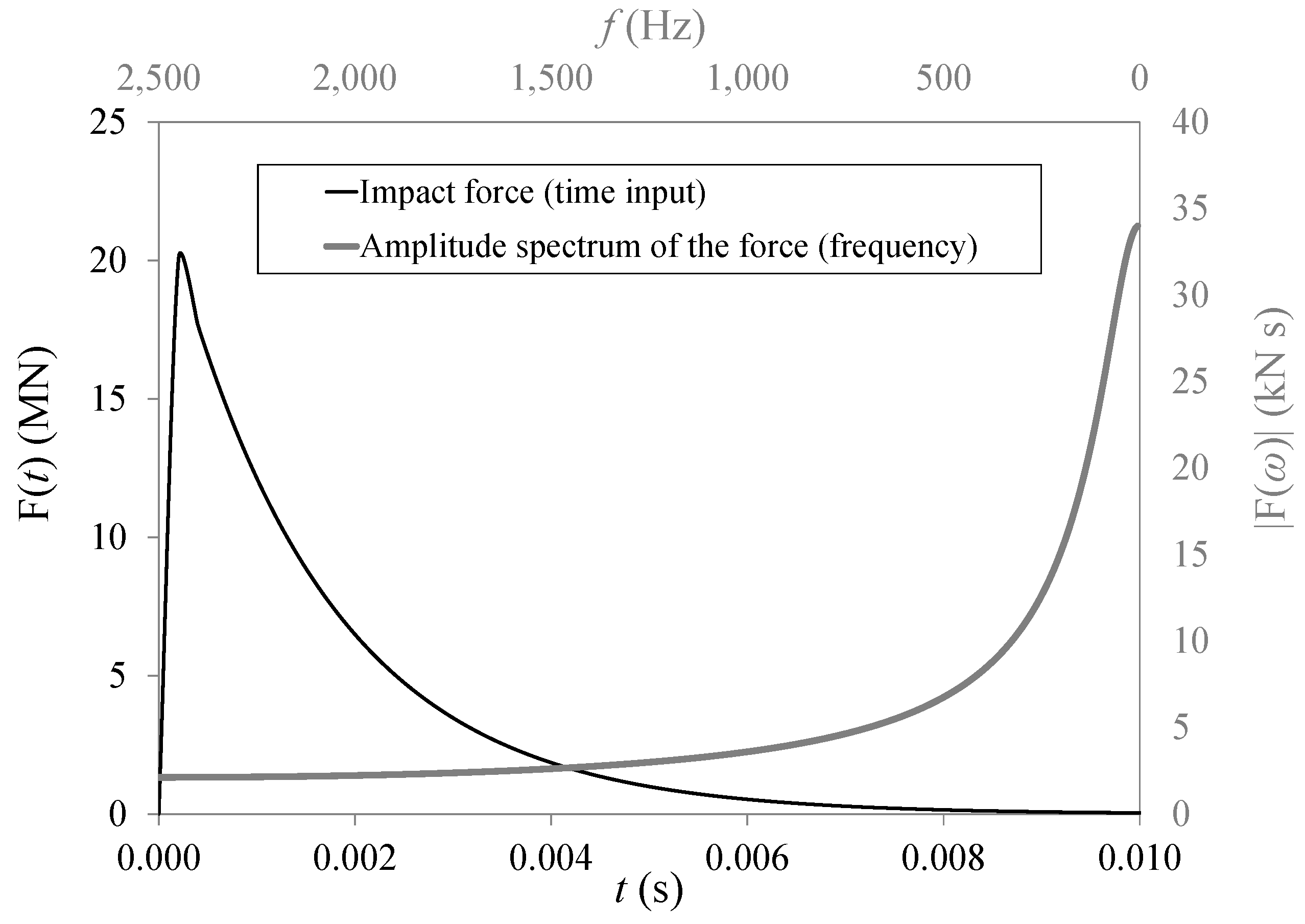
3. Wave Radiation during Installation with an Impact Hammer

This section discusses the noise generated during the installation of a foundation pile with the use of an impact hammer. The considered case corresponds to a typical installation of a large foundation pile in the North Sea. The geometrical and material properties of the pile, as well as those of the surrounding acousto-elastic domain are summarized in

Table 1. Material constants and geometrical parameters of the system in accordance with Figure 1.

Parameter	Value	Unit
E	210,000	MPa
ν	$0.28$	-
ρ	7850	kg·m−3
R	$2.5$	m
L	$58.0$	m
$2h$	$0.05$	m
$z_0$	$5.0$	m
$z_1$	$25.0$	m
$z_2$	$33.0$	m
H	$90.0$	m

and

Table 2. Acousto-elastic waveguide consisting of three layers (from top to bottom): water column, fine sand layer and a sand-clay-silt layer.

Layer	Depth	ρ	${\mathit{c}}_{\mathit{L}}$	${\mathit{c}}_{\mathit{T}}$	${\mathit{\alpha }}_{\mathit{p}}$	${\mathit{\alpha }}_{\mathit{s}}$
	m/m	kg·m−3	ms−1	ms−1	dB/λ	dB/λ
Water	20	1023	1453	−	−	−
Fine sand	8	1900	1797	113	$0.72$	$1.69$
Sand-silt-clay	57	1780	1635	175	$0.49$	$2.27$

, respectively.

The marine sediment is modeled as a two-layered elastic continuum with modified properties to account for water saturation based on the previous studies of Hamilton [37] and Buckingham [38,39]. The values ${\alpha }_p$ and ${\alpha }_s$ designate the attenuation of the compressional and shear waves in each layer. The obtained values of the shear and compressional wave attenuation in the soil medium are similar to those adopted in Table III of [31], representative of the soil conditions in the German North Sea. The soil sediment is divided into two layers, namely, an upper thin layer of water-saturated fine sand with a thickness of 8 m and a stiffer bottom layer compiled of a mixture of sand, clay and silt. The modeling approach adopted by the authors for the soil is seen as a fair compromise between the acoustic modeling approach adopted by most authors nowadays [14,16,17] and the dynamic poroelasticity theory of Biot [40,41]. For an extensive discussion on this subject, the reader is referred to [35].

The force exerted by the impact hammer at the top side of the pile is shown in Figure 2. The total duration of the main pulse is $0.007$ s, and the hammer input energy of a single blow is about 2000 kJ. In reality, the force that is exerted by the hammer will depend strongly on the hammer properties and the pile-hammer interaction characteristics. Despite the fact that the internal structure of the hammer and the choice of the anvil (and/or cushion) will largely define the exact time trace of the exerted force, the overall shape is expected to be similar to the one adopted in this study. The duration and amplitude of the exerted force may, naturally, vary, but this will not affect the qualitative characteristics of the structure-borne wave field discussed hereafter. As can be seen, the bulk of the inserted energy is concentrated at frequencies below $0.5$ kHz. However, it is important to note that the inclusion of the high-frequency tail of the energy spectrum, i.e., $f>700$ Hz, can be significant for acoustic predictions, since it largely defines the peak value of the pressure in the seawater region.

In Figure 3, the radiated waves at the exterior to the pile region generated during a single impact of the hammer are shown for radial distances up to 20 m. The top part (in green-colored background) shows the evolution of the pressure field in the seawater, whereas the bottom part shows (in red-colored background) the velocity norm in the soil medium, i.e., ${\nu }_s(r,z,t)=\sqrt{{\nu }_{s,r}^2(r,z,t)+{\nu }_{s,z}^2(r,z,t)}$. In the soil, both compressional and shear wave fronts are generated. Their inclination (with respect to the pile vertical axis) depends on the ratio of the velocities between the waves in the pile and the correspondent waves in the soil region. In this particular case, the inclination of the compressional fronts has been estimated to be ${19}^{\circ }$ and ${17}^{\circ }$ for the upper and lower soil layers, respectively. The inclination of the shear wave fronts equals $1^{\circ }$ and $2^{\circ }$ for the upper and lower soil layers (almost cylindrical spreading of waves around the pile), respectively. In addition, solid-fluid interface waves (Scholte waves) are visible at later moments in time, which propagate along the fluid-solid interface.

The field in the seawater region consists of pressure waves that span the entire depth of the seawater column (primary noise path). These waves are generated by the oscillation of the surface of the shell as the wave train propagates downwards of the pile and carries energy at a wide range of frequencies. Furthermore, the excited Scholte waves, which propagate along the seabed surface, induce low-frequency pressure fluctuations in the water column close to the seabed level (secondary noise path). These low-frequency waves are clearly distinguished from the initial pressure cones, since they penetrate only slightly into the water zone and propagate at very low speeds.

To investigate further the acoustic field in the seawater region, the evolution of the pressure is shown in Figure 4. The left figure shows the response $4.8$ m below the sea surface, whereas the right figure the response $0.6$ m above the seabed level. As can be seen, the acoustic field close to the sea surface consists solely of the fast-propagating compressional waves radiated directly by the pile vibration.

In contrast, the acoustic field close to the seabed surface consists of two separate contributions. At the initial moments in time, the compressional waves induce some high-frequency oscillations of the fluid similar to those close to the sea surface. As time advances, the slowly-propagating interface waves (sometimes referred to as elastic waves [27] or seismic waves [42]) induce low-frequency oscillations close to the seabed level. The latter can be of significant amplitude, but do not radiate energy into the seawater column (they are not leaky waves). Due to their localized nature, they disturb a finite part of the water column at the vicinity of the seabed-water interface, and hence, their presence is noticeable only within a distance of a few wavelengths from the seabed level. In the right side of Figure 4, they appear after $0.20$ s. In [26], their presence is verified by measurements of geophones positioned on the seabed. Recent studies in the German North Sea [42] have also confirmed their presence at large distances from the construction site and for piles of similar dimensions. At $r=25$ m, the peak pressure associated with the Mach wave radiation is still noticeable for the point positioned close to the seabed surface, while it is largely absent for the point close to the sea surface. This is caused by the fact that at this distance, the top point falls outside the horizontal range influenced by the powerful pressure cone radiated by the first downwards propagating wave train along the pile [26].

Although the horizontal range of influence of the interface waves is generally unknown, since it strongly depends on the contrast of the material properties between the seawater and the upper soil layer, their presence needs to be accounted for when the focus is placed on the design of noise mitigation equipment or when the marine ecosystem is considered particularly rich close to the seabed, i.e., demersal and benthic zones of the water-seabed column. To the best of the authors’ knowledge, the effect of the Scholte waves generated by marine piling is very often overlooked in practice.

Finally, the noise levels are plotted versus the radial distance from the pile in terms of the sound exposure level ($\mathrm{SEL}$) and the absolute maximum of the zero-to-peak pressure level (${\mathrm{SPL}}_{peak}$), which are defined as follows:

$$\mathrm{SEL}=10{log}_{10}\left(\frac{1}{t_0}\underset{t=t_5}{\overset{t=t_{95}}{\int }}\frac{p^2\left(t\right)}{p_0^2}dt\right)$$

(18)

$${\mathrm{SPL}}_{peak}=20{log}_{10}\left(\frac{max\left|p\right(t\left)\right|}{p_0}\right)$$

(19)

In Equations (18) and (19), $p_0={10}^{-6}$ Pa and $t_0=1$ s, while $p\left(t\right)$ corresponds to the predicted (or measured) time trace of the pressure at a predefined position. In Figure 5, the ${\mathrm{SPL}}_{peak}$ in dB re 1 $\mathsf{\mu }$Pa and the SEL in dB re 1 $\mathsf{\mu }$Pa² s are plotted versus the distance from the pile surface for two points positioned at two water depths. As can be seen, the pressures close to the seabed surface are higher than the ones a few meters above it due to the additional presence of the Scholte waves.

4. Validation of the Model Predictions

An experimental case verifying the existence of the Scholte waves for a pile with a diameter of $0.92$ m is discussed extensively in [26]. This case, although useful for validation purposes, cannot be compared to the one presented here due to considerable differences in the system parameters, i.e., pile dimensions, soil conditions and water depth. In this section, predictions of the model are compared to data available in the literature from three measurement campaigns [17,31,42] and one theoretical benchmark case study [43]. In the cases referring to offshore measurements [17,31,42], the time history of the applied force is not always known. However, the input energy of the impact hammer is always mentioned together with the remaining system parameters, and therefore, a rough comparison with the model predictions is possible. For the benchmark case [43], the time history of the input force is explicitly provided by the authors, and therefore, a more complete quantitative comparison of the noise levels is considered.

4.1. Reference Measurement at the Anholt site in the Baltic Sea

The measurement campaign is described in detail in [17]; here, only a brief outline of the main system characteristics is given. The water depth is approximately 18 m, and the pile dimensions are $D=5$ m and $L=45$ m. This case is similar in terms of pile size, water depth and soil conditions to the one investigated in this paper with the only difference being the energy input of the impact hammer, which is about 350 kJ. This energy input is $5.71$-times smaller than the one analyzed in Section 3. As already mentioned, the exact time trace of the applied hammer force at the top of the pile is not provided by the authors in [17], and therefore, it is assumed that the force introduced in Figure 2 (after appropriate scaling) is representative of the actual situation. Assuming that a linear scaling law applies (due to the linear model behavior), one needs to scale down the predicted peak pressure level by a factor of $5.71$ to match it with the measurements (in fact, a computation with a force reduced by a factor of $5.71$ in amplitude would yield the exact same answer). Given that, the scaled (absolute maximum) pressure $p_{sc}$ should be equal to $p_{in}/5.71$, where $p_{in}$ corresponds to the maximum zero-to-peak pressure predicted at 2000 kJ. By applying Equation (19), the difference in the peak pressures equals: $\Delta {\mathrm{SPL}}_{peak}={\mathrm{SPL}}_{peak}^{in}-{\mathrm{SPL}}_{peak}^{sc}=20{log}_{10}\left(p_{in}/p_0\right)-20{log}_{10}\left(p_{sc}/p_0\right)=20{log}_{10}\left(p_{in}/p_{sc}\right)\simeq 15.1$ dB re 1 $\mathsf{\mu }$Pa. A similar reduction is to be expected for the SEL by using Equation (18), but here, the knowledge of the complete time trace (rather than the peak value alone) is of importance.

In

Table 3. Comparison of noise predictions with measurements [17].

Distance	Quantity	Prediction	Scaled Prediction	Measurement	ΔSEL; $\mathbf{\Delta }{\mathbf{SPL}}_{\mathit{p}\mathit{e}\mathit{a}\mathit{k}}$
(m)		(2000 kJ)	(350 kJ)	(mean value)	-
60	${\mathrm{SPL}}_{peak}$	$221.9$	$206.8$	$207.0$	$-0.2$
	$\mathrm{SEL}$	$199.5$	$184.4$	$184.0$	$+0.4$
750	${\mathrm{SPL}}_{peak}$	$206.9$	$191.8$	$192.0$	$-0.2$
	$\mathrm{SEL}$	$188.2$	$173.1$	$170.0$	$+3.1$

, the results of the measurements at 60 m and 750 m are compared to the predictions of the model (scaled version of Figure 5) at a depth of 2 m above the seabed surface. As can be seen, the predictions are satisfactory with the exemption only in the value of SEL at a distance of 750 m showing a difference of ΔSEL$=+3.1$ dB. However, such differences are to be expected because of: (i) the slightly different geometrical characteristics, i.e., pile length of 45 m (instead of 58 m in the model) and the water depth of 18 m (instead of 20 m in the model); (ii) the uncertainty in the soil properties; and (iii) the simplified form of the input force of the hammer assumed in the model.

4.2. Offshore Wind Farm in the German North Sea

The case analyzed in [42] corresponds to a hammer input energy of 800 kJ, which is about 40% of the input energy of the one examined in Section 3. Assuming a linear behavior of the system, a conversion factor of $0.4$ could be applied to the predictions in order to scale them down to an input energy of 800 kJ, as demonstrated previously in Section 4.1. However, the soil conditions in the region correspond to a much stiffer soil with a wave speed of the Scholte waves estimated at 500 ms⁻¹. Such a speed is about five-times larger than the one adopted here, and therefore, the results cannot be compared directly. Since we are interested in the soil vibrations, a new case is simulated with the model presented in Section 2 corresponding to the measurement campaign discussed in [42] for validation purposes.

The pile has the following properties: $D=6$ m, $L=55$ m and $2h=0.055$ m. The water depth equals 21 m, which is within the range of $19.5$–$23.6$ m measured at the offshore location. Due to the lack of more detailed data, a homogeneous soil is assumed with the following properties: $c_L=1707$ ms⁻¹, $c_T=559$ ms⁻¹, ${\rho }_s=2000$ kgm⁻³, ${\alpha }_p=0.5$ dB/λ and ${\alpha }_s=1.0$ dB/λ. With the chosen values of the soil material properties, the speed of the Scholte waves is about $c_{Sch}=530$ ms⁻¹, which is close to the one mentioned in [42].

As the time signature of the force is generally unknown, the comparison of the results focuses mainly on: (i) the peak values of the various physical quantities; and (ii) the qualitative characteristics of the radiated wave field. In addition, in some of the measurement results presented in [42], hydro sound dampers (HSD) are applied for noise reduction. Although such a mitigation system can effectively reduce the noise radiated directly into the water by the pile vibrations, i.e., primary noise path, its influence on the secondary noise path is found to be minimal. This allows us to compare the computed and measured soil vibrations. A comparison of the amplitudes of the waves corresponding to the primary noise path should, however, take into account the reduction of the high-frequency noise due to the application of the HSD.

In Figure 6, the computed vertical velocity is shown at the surface of the seabed and at three distances from the pile (left plot) together with the correspondent amplitude spectra at the same positions (right plot). These graphs can be compared to the ones presented in Figure 7 of [42]. The following conclusions can be drawn.

First, the qualitative picture of the measured velocities by the geophones positioned on the seabed surface (Figure 7 in [42]) is similar to the one computed in Figure 6. In [42], the primary noise path contains additionally energy at much higher frequencies compared to the case analyzed here (Figure 6). This difference is mainly caused by the different force applied at the pile head. In reality, the force is not a smooth exponential function of time (as the one assumed here), but contains energy at higher frequencies associated with the acceleration of the various masses of the impact hammer, which strike the pile head at various time moments. Thus, in real applications, the ascending and descending branches of the force-time plot are non-smooth, and therefore, energy is introduced at higher frequencies. However, the amplitude of the vertical velocity, as well as its attenuation at increasing horizontal distance from the pile is comparable to the measurements. It seems that the model here slightly overestimates the amplitude of the interface waves. For example, in [42], the following amplitudes are measured: $\simeq 2$ mms⁻¹ and $\simeq 1$ mms⁻¹ at a distance of 70 m and 140 m, respectively. The computed values are $6.1$ mms⁻¹ and $1.2$ mms⁻¹ at the same distances. Given the uncertainty in the estimation of several system properties (including the input force), such deviations are to be expected. The overestimation of the vertical ground motions may also be attributed to the assumed non-slip contact condition between the pile and the surrounding soil. When formulating the pile-soil interface conditions, a kinematic constraint is imposed resulting in equal pile and soil displacements in both the radial and vertical directions along the pile shaft, i.e., Equation (12). In reality, the two surfaces are allowed to separate, which effectively results in a reduced amount of energy passing into the vertically-polarized shear waves in the surrounding soil medium. Consequently, less energy is expected to radiate along the seabed-water interface in the form of Scholte waves. However, as discussed in [31], such a simplification is reasonable in noise predictions, and the differences are not expected to be large.

Second, the amplitude spectrum of the measured vertical velocity on the surface of the ground at the predefined locations, i.e., Figure 7 in [42], shows that the energy carried by the interface waves is concentrated at frequencies of around 10 Hz with very limited amounts of energy above 50 Hz. The model (Figure 6) computes energy at similar frequency ranges, albeit with an extra noticeable peak around 20 Hz close to the pile. Such differences are again to be expected given the uncertainty in the soil modeling properties and the force input. Qualitatively, however, the predictions capture the general trend of the measurements in terms of both peak values and wave attenuation characteristics.

As complementary to the ground velocities, the ${\mathrm{SPL}}_{peak}$ and $\mathrm{SEL}$ are plotted versus the distance from the pile surface in Figure 7. The ${\mathrm{SPL}}_{peak}$ at the middle of the water column and at a distance of 15 m is estimated to about 206 dB (Figure 4 in [42]). The computed value equals ${\mathrm{SPL}}_{peak}=209$ dB at that same position. At a distance of 140 m the measured and computed values are ${\mathrm{SPL}}_{peak}=195$ and ${\mathrm{SPL}}_{peak}=191$, respectively.

4.3. Reference Measurement at the Bard Offshore 1 Construction Site

The measurement campaign described in this subsection is used for validation of the numerical model described in [31] and includes both near- and far-field measurements of the acoustic field. The pile has a length of 85 m, a diameter of $3.35$ m and a mean wall thickness of approximately 7 cm. The water depth at the installation site was approximately 40 m. During the reference measurement that is used for validation purposes, the actual penetration length of the pile into the soil was about 20 m. The pile was driven using a MENCK MHU 1900 S hydraulic hammer with a ramp energy of about 1370 kJ. The sound pressure level at a distance of 10 m from the pile and at mid-water depth is used for the near-field validation. The sound pressure level at 1500 m and a height of 2 m above the seabed is considered for the far-field model validation. The soil properties assumed are summarized in Table III of [31]; here, only the properties of the upper two layers are considered in the simulation. The time history of the applied force is provided in Figure 9 of [31] together with the corresponding spectra density levels. The input force applied in our case is shown in Figure 8. This pulse is similar in duration, shape and amplitude to the main pulse measured in [31]. In fact, the data provided for this measuring campaign are complete since all of the material and geometrical characteristics are given (also the penetration depth of the pile into the soil), as well as the measured force applied at the head of the pile. Therefore, a full quantitative comparison of the results is possible.

The variation of the ${\mathrm{SPL}}_{peak}$ and $\mathrm{SEL}$ as function of the distance from the pile and at two depths is shown in Figure 9. The results at the two measurement locations are summarized in

Table 4. Comparison of noise predictions with measurements [31].

Distance	Depth	Quantity	Computed	Measured [31]	ΔSEL
10	20	$\mathrm{SEL}$ (dB re 1 $\mathsf{\mu }$Pa s)	$198.1$	$197.5$	$+0.6$
1500	38	$\mathrm{SEL}$ (dB re 1 $\mathsf{\mu }$Pa s)	$177.1$	$174.6$	$+2.5$

. As can be seen, the model can reproduce the measurements with sufficient accuracy given the uncertainties associated with the modeling of the actual environment and the small difference in the time history of the applied force. The maximum difference in the SEL value equals $+2.5$ dB at a radial distance of $1.5$ km from the pile, whereas the agreement with the near-field measurement at 10 m is remarkably good. The computed values with the model presented in [31] equals $198.3$ dB and $176.1$ dB at a distance of 10 m and 1500 m, respectively. These values deviate from the predictions of the current model by $-0.2$ dB and $+1$ dB, respectively. Thus, it can be concluded that when the system characteristics are well defined, i.e., pile dimensions and penetration depth, soil properties and hammer input force, the predictions of the model can be very accurate.

4.4. Theoretical Benchmark Case: COMPILE

The last case analyzed here corresponds to the one presented in [43]. It is a benchmark case study developed for the validation of models used for noise predictions from pile driving. For this reason, it does not correspond to a real application as the previously examined cases. However, it is of particular interest, since it gathers predictions of several numerical models developed for the same purpose.

The model consists of a pile with a length of $L=25$ m, a diameter of $D=2$ m and a wall thickness of $t=0.05$ m, which is embedded 15 m into the seabed. The water depth is assumed equal to 10 m. The hammer force is shown in Figure 10 together with the amplitude spectrum. The densities and sound speeds in the water and in the sediment are equal to: $c_w=1500$ ms⁻¹, $c_L=1800$ ms⁻¹, ${\rho }_w=1025$ kgm⁻³ and ${\rho }_s=2000$ kgm⁻³. In addition, a shear wave speed is allowed in our model, which is assumed equal to $c_T=170$ ms⁻¹. The attenuation of compressional and shear waves in the soil is assumed equal to ${\alpha }_p=0.47$ dB/λ and ${\alpha }_s=1.69$ dB/λ, respectively. Due to the explicit incorporation of shear rigidity in the soil description, the extra attenuation in the embedded length of the pile considered in [43] is omitted.

First, the pressure time series computed for two points positioned at $r=11$ m, $r=19$ m and at $z=5$ m are shown in Figure 11. The maximum zero-to-peak computed pressure at a distance of 11 m equals $88.5$ kPa, which is very close to the value predicted by several other models (see Figure 3 in [43]). The continuous reflections of the waves at the head and the tip of the pile results in the radiation of several pressure cones in the surrounding fluid medium in the close range, as predicted by almost all models (except the JASCO model [44] which is a time-domain finite difference model in which the pile is modeled as a thin cylindrical shell; the energy dissipation in the sediment is accounted for by using an impedance boundary condition, and a wave reflection coefficient determines the amplitude of the stress waves reflected from the tip of the pile) in [43] in which the soil is described by an equivalent fluid model. The number of continuous wave reflections predicted by the present model is reduced. Since shear frictional resistance is explicitly accounted for at the pile-soil interface, the bulk of the energy carried by the wave train traveling downwards of the pile is radiated away in the form of vertically-polarized shear waves in the surrounding soil medium. Subsequently, less energy is left to irradiate in the form of pressure waves in the water region. However, the amplitude of the first pressure peak originating by the wave train traveling downwards of the pile surface is largely unaffected by the soil modeling; the computed value deviates only by $\Delta {\mathrm{SPL}}_{peak}=+1.4$ dB re 1 $\mathsf{\mu }$Pa from the average value computed by other models.

The predictions of the model are then compared to the benchmark values in terms of the broadband sound levels at three distances from the pile surface and at various depths, as shown in

Table 5. Comparison of noise predictions of the model with the COMPILEbenchmark case study [43].

Distance	Depth	Quantity	Present Model	Ref. [43]	$\mathbf{\Delta }{\mathbf{SPL}}_{\mathit{p}\mathit{e}\mathit{a}\mathit{k}}\mathbf{;}\mathbf{\Delta }\mathbf{SEL}$
11	5	${\mathrm{SPL}}_{peak}$	$218.9$	$217.5$	$+1.4$
11	5	$\mathrm{SEL}$	$186.3$	$n/a$	−
750	9	${\mathrm{SPL}}_{peak}$	$193.3$	$191.0$	$+2.3$
750	9	$\mathrm{SEL}$	$169.4$	$167.0$	$+2.4$
1500	9	${\mathrm{SPL}}_{peak}$	$188.2$	$184.5$	$+3.7$
1500	9	$\mathrm{SEL}$	$165.0$	$161.0$	$+4.0$

. Due to the fact that in [43], six different models are discussed, we choose here the average computed value as retrieved from Figures 3 and 5 of [43]. As can be seen, the predictions of the present model lie close to the average value computed by the other models despite the different modeling of the soil and pile-soil interaction. The overestimation of the noise levels close to the seabed surface is attributed to the difference in the soil description (elastic in our model versus acoustic in the other cases); the soil description modifies the vibration of the shell itself because of the explicit consideration of the shear frictional resistance along the pile shaft. This in turn influences the radiation of sound, especially when the waves are reflected from the tip of the pile. In [43], this is indirectly accounted for by an increased attenuation in the fluid model description of the sediment for the energy lost into shear waves or by the use of an impedance boundary description. Given the difference in the modeling of the soil, the deviations between the model predictions are explicable. For example, the JASCO model [44], which uses a different approach to account for the soil modeling in comparison with the other models, provides slightly different results, especially regarding the wave radiation pattern resulting from the reflected waves from the tip of the pile. This proves the importance of the soil modeling when high accuracy computations are needed (including thus correct estimation of the amplitudes of the reflected waves).

4.5. Concluding Remarks

In this section, a comparison of several model predictions with measurements has been presented. Given (i) the uncertainty in the modeling of several system parameters, (ii) the simplifications associated with the modeling of the pile and the acousto-elastic waveguide (in reality, the seabed and the various soil layers are not horizontal; the sea surface is not an ideal pressure release boundary; the properties of the waveguide can vary continuously with depth and range; and the hammer-pile interaction needs to be considered) and (iii) the limited data provided regarded the input force in some of the examined cases, the predictions of the model can be regarded as reliable. In addition, the comparison with the benchmark case study [43] shows that the model can provide reliable predictions at both the near- and far-field noise levels.

5. Noise Prediction during Installation with a Vibratory Device

In this section, the noise field is investigated for the case of a foundation pile installed with a vibratory hammer. Although the studies on this subject are limited [28,29], the current trend of the wind industry towards the use of vibratory hammers of larger dimensions may lead to increased environmental concern regarding the generated underwater noise. The pile and soil properties are already given in Section 3. The force applied at the top side of the pile is shown in Figure 12. It has a maximum amplitude of 10 MN, a primary frequency component of 20 Hz and energy distributed among several sub- and super-harmonics.

The radiated wave field in the soil and in the seawater is shown in Figure 13. The wave pattern is different from the one presented previously for the case of the installation with an impact hammer. The following points are worth mentioning.

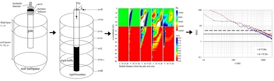
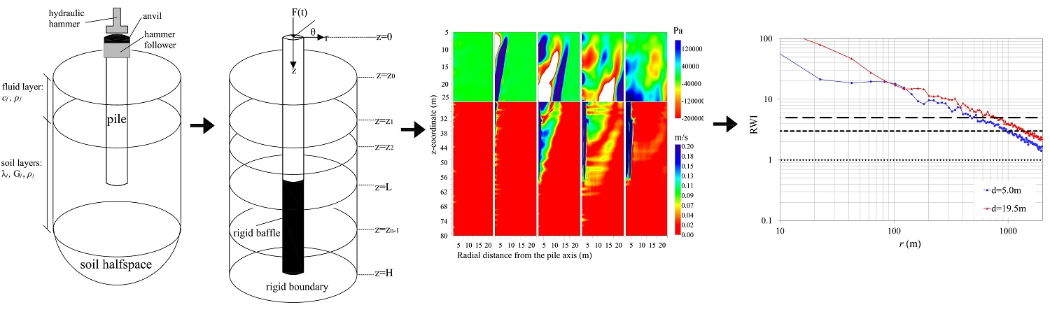
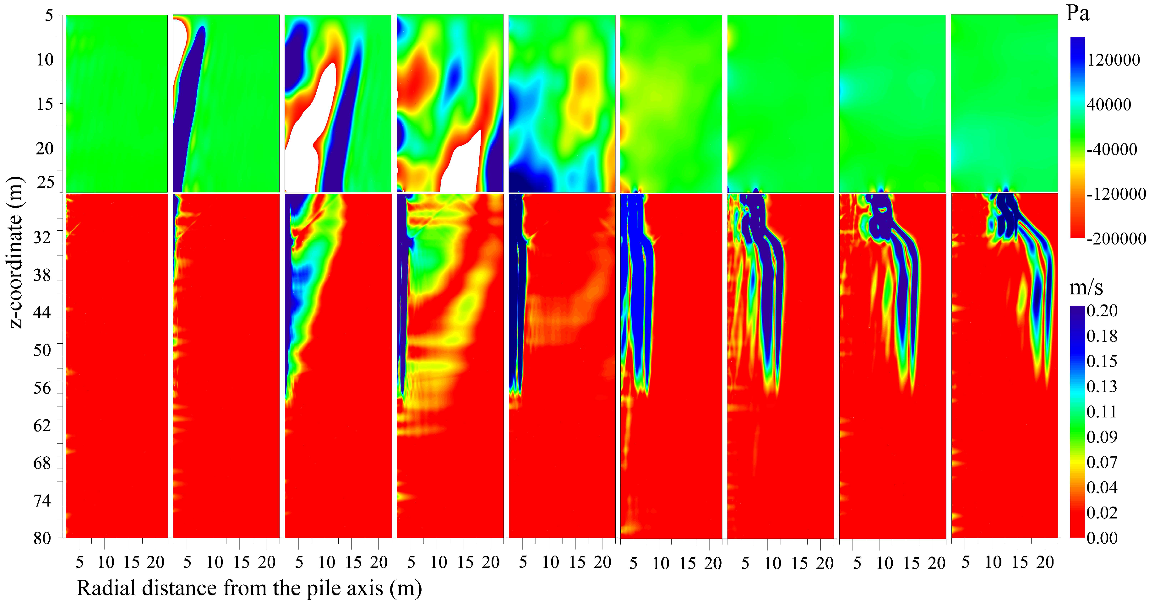
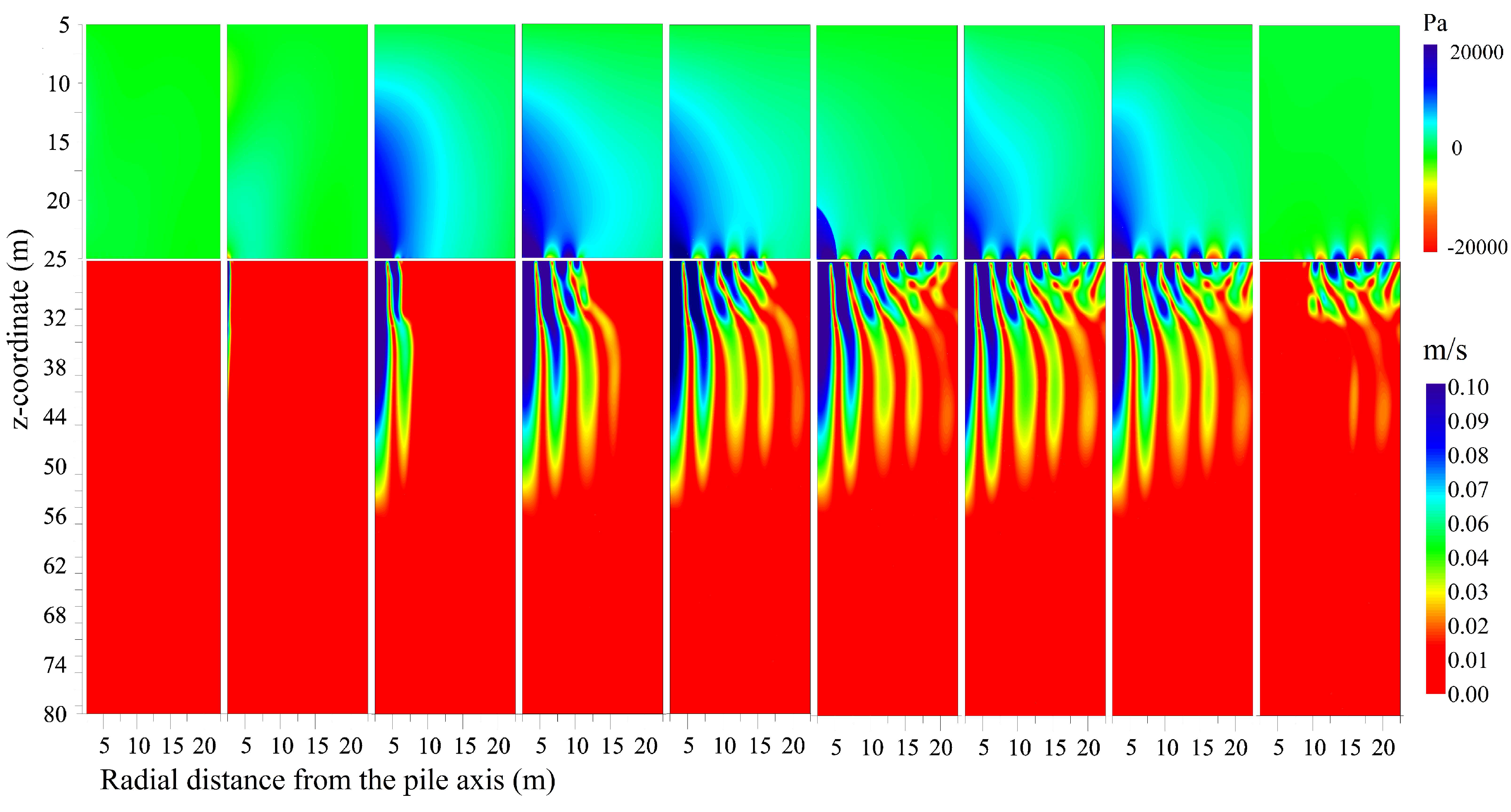
• The response of the system reaches a steady-state regime after a few loading cycles. Here, only a limited number of loading cycles is investigated (nine in total) in order to show the radiated wave pattern and the generated acoustic field. In reality, thousands of loading cycles are needed to install a single pile, and the same response will continue unaltered for longer periods of time.
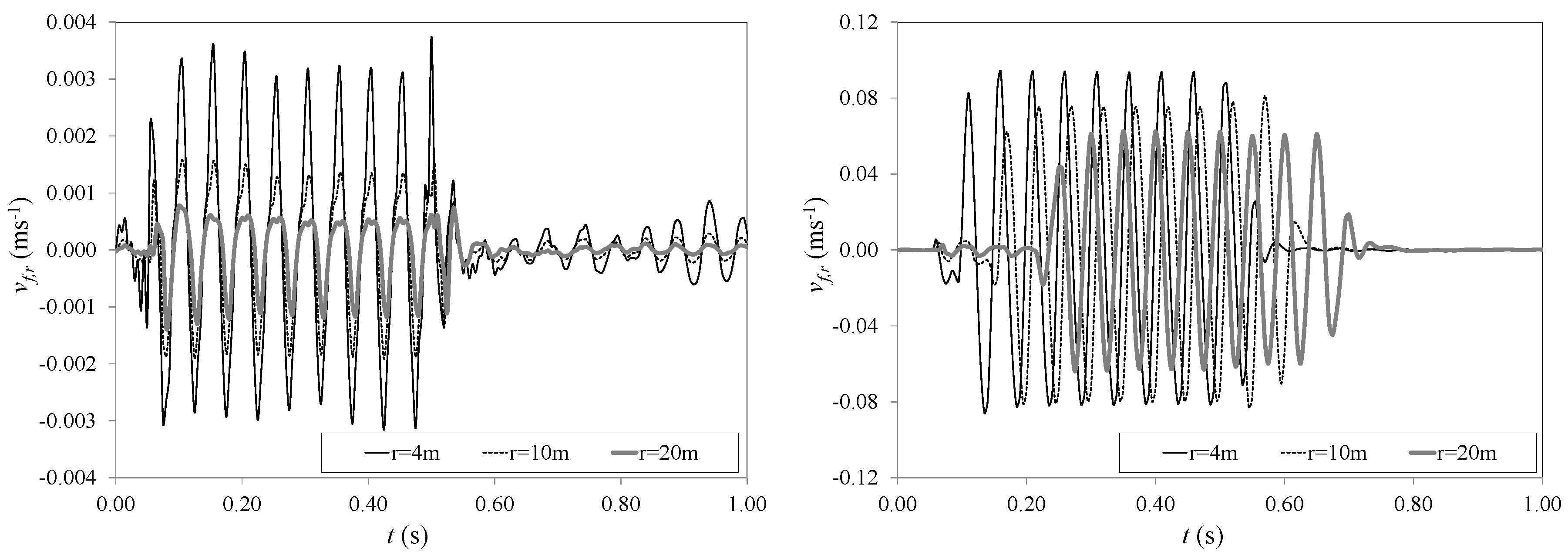
• The wave field in the soil consists of vertically-polarized shear waves with almost cylindrical fronts that propagate outwards from the vibrating pile with the shear wave velocity in each soil layer. As time advances, the waves in the bottom soil layer are separated from the ones at the upper soil layer due to the difference in the shear wave speed between the two layers, i.e., $c_{T,2}>c_{T,1}$. This results in an upward bending of the shear fronts at the interface of the two soil layers, which is clearly visible at $t>0.15$ s.
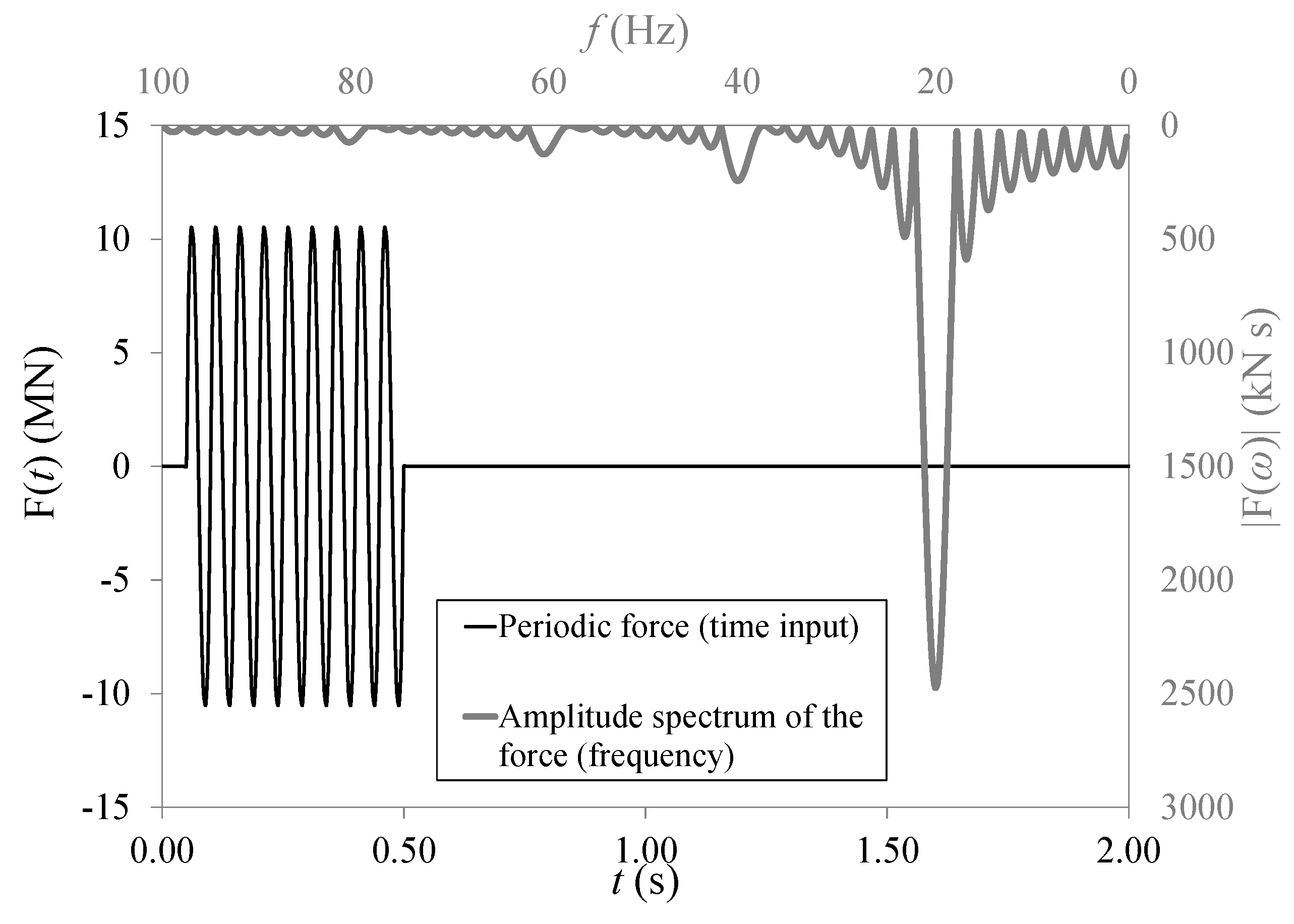
• The Scholte waves, which propagate parallel to the seabed-water interface, attenuate much less in comparison to the shear waves in the soil. In addition, despite the fact that the maximum amplitude of the exerted force at the top of the pile is reduced by a factor of 20, when compared to the one exerted by the impact hammer (Section 3), the amplitude of the Scholte waves is reduced only by a factor of six. This is related to the fact that the soil responds mainly at low frequencies, which dominate the response in the case of vibratory piling.
• The highest pressures are predicted close to the seabed surface. The typical Mach wave radiation pattern in the fluid region (primary noise path) is not observed in this case. This is in line with the observations and the model developed by Dahl et al. [29] in which the vibratory pile source is modeled as an incoherent line source (and not as a coherent one with a predefined time delay, as was the case when impact piling was examined). As mentioned in [29], any sense of line-source spatial coherency is lost or at the very least rendered vastly more complex with effects not observable in the ensuing pressure field. In other words, the Mach wave radiation from a coherent source traveling down the pile surface is not seen in the case of vibratory piling. On the contrary, the secondary noise path, which consists of the Scholte waves, seems to govern the noise field in the seawater at low frequencies in the vicinity of the seabed surface. This is again in line with the measurements presented in [29], albeit for a different installation setup and pile dimensions, in which it was observed that the Scholte mode contributes to more than 30 dB in the 63-Hz octave band.
• The pressures in the water column are significantly lower when compared to the ones generated by the impact hammer. At this low frequency range, only a few modes propagate in the seawater, i.e., the bulk of the energy irradiates into the soil domain. The contribution of the few propagating modes into the fluid region and its experimental identification are discussed extensively in [29].

In Figure 14, the evolution of the radial velocity component is shown at two depths in order to highlight the contribution of the Scholte waves close to the seabed-water interface. As can be seen, the radial velocity close to the sea surface is significantly lower compared to the one close to the seabed. The latter is clearly governed by the presence of the interface waves. Thus, in the case of vibratory pile driving, the pressures are expected to be higher close to the seabed surface.

6. Zones of Impact for the Aquatic Species

The evaluation presented hereafter combines the results obtained in Section 3 with relevant studies of marine biologists regarding the onset of injury on aquatic species from exposure to impulsive sounds [30]. The environmental problem related to underwater noise generated by offshore pile driving needs the combined effort of several specialists in order to: (i) quantify the noise levels; (ii) assess the possible negative impact on the marine species; and (iii) propose efficient methods to eliminate the problem. These three aspects of the problem are strongly interrelated. Studies on the third aspect mentioned above do exist, but do not form part of our discussion in this paper. Most of the previous studies on the subject focus on the first aspect and, thus, leave the second one largely intact. Nevertheless, the extent to which offshore pile driving influences the aquatic environment remains a very important issue. It requires a good understanding of the primary characteristics of the underwater noise associated with pile driving (impulsive characteristics, principal frequency content of the radiated sound, etc.) and a certain knowledge of the auditory behavior of the marine species when subjected to noise of increasing intensity levels. In this section, a method is presented to convert the levels of noise to a single index that can be used for the design of zones of impact in offshore regions where pile driving activities are planned in the future. The method is not restricted to the single species discussed hereafter in the sense that once more data become available on the cumulative effects of pile driving in other aquatic species, i.e., marine mammals or fish, they can be used to define zones of impact around the installation site in a similar way.

6.1. Impact of Pile Driving Noise on Fish

Before continuing further, we briefly address the studies of biologists on the subject. In this context, we do not adopt the so-called equal energy hypothesis (EEH), which has been suggested by several specialists as a suitable metric for the mitigation of the effects of impulsive sounds on fish [45,46,47]. The baseline of this hypothesis is that the influence on the marine species depends on the total energy radiated into the water region during pile driving, regardless of how this total energy is accumulated in time, i.e., a few strikes of high energy or a larger number of strikes of relatively low energy. On the contrary, we adopt a method that is based on the individual sound exposure levels (SEL) as a result of each individual blow of the hammer and the cumulative SEL resulting from the total number of blows during the installation of a foundation pile. As shown in various recent studies on the subject, such an approach seems to be more suitable for sounds of impulsive character [30,48,49], differentiating between the levels of noise generated by a single blow and the way in which the cumulative energy levels are compiled. The EEH method, however, may still be applicable to cases in which the installation is accomplished with the help of vibratory hammers due to the different nature of the radiated sound. In this section, the discussion is limited to the case of installation with impact hammers, which is expected to be more governing in terms of noise pollution. In the following subsections, two pile installation scenarios are first discussed, and the zones of impact for each of those are subsequently defined.

6.2. Pile Driving Scenarios

Two pile driving scenarios are considered regarding the input energy of the hydraulic hammer and the number of blows needed to reach the final penetration depth:

• First scenario: The energy input of the hydraulic hammer equals 1000 kJ, and 2000 strikes are required to install the pile;
• Second scenario: The energy input of the hydraulic hammer doubles, i.e., 2000 kJ, and only 1000 strikes suffice to reach the final penetration depth.

In both cases, the configuration of the pile is shown in Figure 1 with the waveguide properties taken from Table 2. This case can be considered representative of the installation of a large foundation pile in the North Sea. It is important to mention that the sound exposure level (SEL) changes in the two scenarios due to the different input energy of the impact hammer. Ideally, one should also account for the effect of the soil penetration depth, as well, but for this first analysis, we limit ourselves to the aforementioned installation configurations for simplicity. To properly account for the influence of the changing penetration depth of the pile into the soil, one can consider several stages during the installation phase, which differ only by the penetration depth, and perform a separate analysis for each of those with the defined impact force. The SEL can then be estimated for each separate configuration by Equation (18) and converted to a cumulative SEL by Equation (20). The range-dependent response weighted index (RWI) can subsequently be calculated from Equation (21).

For the two adopted scenarios, the SEL and the ${\mathrm{SPL}}_{peak}$ are first estimated at several horizontal distances from the surface of the pile and at two depths. One of the positions is chosen close to the seabed surface based on the findings of Section 3 and Section 4. The pressure levels predicted on the seabed surface were higher than elsewhere in the water column because of the additional contribution of the Scholte waves. Thus, it is expected (and in fact, verified by several measurement campaigns to date) that the SEL values calculated close to the seabed will constitute an upper conservative limit of the SEL throughout the water column. Subsequently, the SEL from the individual pile strikes is transformed into a cumulative SEL accounting for the total number of strikes needed for the installation of a single pile using the following expression:

$${\mathrm{SEL}}_{cum}=\mathrm{SEL}+10{log}_{10}\left(N\right)$$

(20)

${\mathrm{SEL}}_{cum}$ denotes the cumulative SEL, and N is the number of strikes needed to install the pile. Finally, the cumulative SEL is transformed into a range-dependent response weighted index (RWI) following the related work of [30] as follows:

$$\mathrm{RWI}=exp(-30.05+0.149{\mathrm{SEL}}_{cum}-0.000171N)-1$$

(21)

The latter can be used as an index for specifying zones surrounding the pile that define different injury levels for specific types of fish. Naturally, the choice of appropriate indices of damage for the aquatic species is not an easy task and contains large uncertainties. The RWI considers the combined effect of the sound exposure level (SEL) given by Equation (18), together with the total number of strikes needed to install a single pile. In this respect, it attempts to model the biological effects on the marine species. Since the studies on the subject are rare, we limit ourselves to the case discussed in [30], which focuses on the analysis of the behavior of the Chinook salmon (Oncorhynchus tshawytscha) subjected to impulsive sounds generated by an impact hammer striking a steel pile. Obviously, a similar approach can be followed for other species, as well, once more data become available. An RWI index of one implies only some minor injury (mild trauma); an index of three suggests moderate injury; and an index of five implies a mortal injury (death within an hour of exposure). With the RWI, different zones of impact can be established at certain distances from the pile surface.

In Figure 15, the ${\mathrm{SPL}}_{peak}$ and the SEL are plotted versus the distance from the pile surface at two water depths for the first installation scenario. As can be seen, the pressures close to the seabed surface are generally higher than the ones a few meters above it. A comparison of these values with the allowable values of the ${\mathrm{SPL}}_{peak}$ (190 dB re 1 $\mathsf{\mu }$Pa) and the SEL (160 dB re 1 $\mathsf{\mu }$Pa² s) at a distance of 750 m given by the German regulations [12] shows that both values exceed the allowable ones in this specific case.

In Figure 16, the RWI is calculated for the two positions along the depth of the water and plotted versus the horizontal distance from the pile surface. According to the computed values, mortal injury of the Chinook salmon is to be expected up to a horizontal distance of $r=800$ m from the pile surface, whereas moderate injury is expected up to a distance of $r\sim 1200$ m. Obviously, the critical point is the one positioned closer to the seabed surface. For larger horizontal distances, i.e., $r>10$ km, the effects on the specific species are expected to be minor.

In Figure 17, the RWI is plotted for the second installation scenario in which the energy of the hydraulic hammer is doubled, i.e., 2000 kJ, whereas the number of blows needed to install the pile is halved ($N=1000$). The levels of mortal injury and moderate injury are shifted towards larger horizontal distances, which actually implies that the zones of impact for the Chinook salmon are altered. Thus, it is the combined effect both of the level of noise (SEL) and of the way in which the total energy is inserted into the system (number of hammer strikes) that define the RWI and, consequently, the auditory damage of the hearing abilities of the species. Hence, different installation configurations can yield different zones of impact for specific aquatic species. In contrast to the specification of ${\mathrm{SPL}}_{peak}$ and SEL as the design criteria, a more global approach seems to be advisable, which would allow for the differentiation of the levels of damage depending on both the energy input by an individual hammer blow, as well as on the way in which the total energy is accumulated in the system during the installation of a single pile.

The results presented in Figure 16 and Figure 17 refer to a theoretical case study of the installation of large foundation piles with impact hammers in the North Sea. This study aims to present a way of integrating the quantitative predictions of existing models into environmental assessment studies and not to reach conclusions about the mortality of certain marine species. The specific species were used here only as a reference case because laboratory studies were available. For this reason, the authors did not investigate whether the considered species (Chinook salmon) are native in the North Sea (probably, they are not). In addition, fish may well evacuate the construction site well before the installation completes, and therefore, the accumulation of hearing damage may be different in actual cases. For our theoretical study, we assumed that the species remain in the region throughout the pile installation process (this being a rather unrealistic assumption), and the conclusions therefore reflect only this situation. Although theoretical, such studies may be more relevant for aquatic species that cannot abandon the installation site quickly, i.e., certain species living at the demersal and benthic zones of the water-seabed column.

6.3. Impact of Pile Driving Noise on Mammals

Although the case studied previously refers to specific fish species, there are cases in which the interest lies mainly in the behavior of marine mammals. A recent study on this subject is presented in [50] in which the focus is placed on: (i) the behavior of certain marine mammals native to the North Sea, i.e., harbor porpoise and seal; and (ii) the derivation of appropriate noise levels to quantify the effects of the installation of piles on those species. Once certain sound level criteria are established based, for example, on the cumulative sound exposure level (${\mathrm{SEL}}_{cum}$), a similar approach can be followed to define zones of impact around the installation site.

7. Conclusions

This paper discusses the noise radiation during the installation of foundation piles for the offshore wind industry. It also employs a method to transform the predicted noise levels to a cumulative damage index in order to define zones of impact around the pile. Two cases are investigated, namely one in which the pile is installed with an impact hammer and one in which the installation is accomplished with the help of a vibro-hammer. It is shown that the wave radiation field is considerably different in the two cases. In impact piling, a transient wave field is generated, which consists of shock waves of relatively high intensity that propagate away from the pile shortly after the hammer impact. The acoustic field in the fluid region is compiled of powerful pressure cones (primary noise path) that span over the entire depth of the fluid column. Thus, the sound field during impact piling consists of multiple impulsive sounds of very high energy. In the soil region, both shear and compressional waves are generated together with Scholte waves that propagate along the seabed-water interface. The latter induce low-frequency pressure fluctuations close to the seabed surface (so-called secondary noise path). On the contrary, the response of the coupled pile-soil-water system in the case of vibro-piling reaches a steady-state regime after a few loading cycles. In this case, the contribution of the soil becomes extremely important since the noise in the water column is the highest close to the seabed due to the additional contribution of the Scholte waves at low frequencies. In contrast to the impact piling, the noise is continuous, and therefore, different criteria are required to access its influence on the surrounding marine environment.

At the last section of the paper, a method is presented to convert the noise levels predicted by the model to an equivalent cumulative damage index (RWI) that reflects the effect on certain marine species. To this end, the analysis is restricted to a theoretical case study of one species only (Chinook salmon) and to the case of an installation with an impact hammer. Two different piling scenarios are considered, which vary with respect to the hammer energy input per blow and the number of blows required to reach the final penetration depth. Results are presented in terms of so-called zones of impact, which define the degree of damage to be expected at a certain distance from the installation site. It is believed that such an approach can be useful to bridge the existing gap between the noise predictions as provided by engineers and the related work of marine biologists on the subject. Once appropriate data become available, the method could be used for defining zones of impact for other aquatic species, as well, i.e., marine mammals or fish.

References

1. The European Offshore Wind Industry—Key Trends and Statistics 2013; Technical report; The European Wind Energy Association: Brussels, Belgium, 2014; Available online: http://www.ewea.org/fileadmin/files/library/publications/statistics/Europeanoffshorestatistics2013.pdf (accessed on 26 July 2016).
2. Gerwick, B.C. Construction of Marine and Offshore Structures, 3rd ed.; CRC Press: San Francisco, CA, USA, 2007; pp. 255–318. ISBN 9781420004571. [Google Scholar]
3. Deeks, A.J.; Randolph, M.F. Analytical modeling of hammer impact for pile driving. Int. J. Numer. Anal. Methods Geomech. 1993, 17, 279–302, ISSN 1096-9853. [Google Scholar] [CrossRef]
4. Wong, D.; O’Neill, M.W.; Vipulanandan, C. Modeling of vibratory pile driving in sand. Int. J. Numer. Anal. Methods Geomech. 1992, 16, 189–210. [Google Scholar] [CrossRef]
5. Bailey, H.; Senior, B.; Simmons, D.; Rusin, J.; Picken, G.; Thompson, P.M. Assessing underwater noise levels during pile-driving at an offshore wind farm and its potential effects on marine mammals. Mar. Pollut. Bull. 2010, 60, 888–897. [Google Scholar] [CrossRef] [PubMed]
6. David, J.A. Likely sensitivity of bottlenose dolphins to pile-driving noise. Water Environ. J. 2006, 20, 48–54. [Google Scholar] [CrossRef]
7. Madsen, P.T.; Wahlberg, M.; Tougaard, J.; Lucke, K.; Tyack, P. Wind turbine underwater noise and marine mammals: Implications of current knowledge and data needs. Mar. Ecol. Prog. Ser. 2006, 309, 279–295. [Google Scholar] [CrossRef]
8. Popper, A.N.; Hastings, M.C. The effects of anthropogenic sources of sound on fishes. J. Fish Biol. 2009, 75, 455–489. [Google Scholar] [CrossRef] [PubMed]
9. Damian, H.-P.; Merck, T. Cumulative impacts of offshore windfarms. In Ecological Research at the Offshore Windfarm Alpha Ventus; Federal Maritime, Hydrographic Agency, Nature Conservation Federal Ministry for the Environment, Nuclear Safety, Eds.; Springer Fachmedien: Wiesbaden, Germany, 2014; pp. 193–198. [Google Scholar]
10. Erbe, C. International regulation of underwater noise. Acoust. Aust. 2013, 41, 12–19. [Google Scholar]
11. Statutory Nature Conservation Agency Protocol for Minimising the Risk Injury to Marine Mammals from Piling Noise; Joint Nature Conservation Committee: Aberdeen, UK, 2010.
12. Werner, S. Towards a Precautionary Approach for Regulation of Noise Introduction in the Marine Environment from Pile Driving; Federal Environmental Agency: Stralsund, Germany, 2010. [Google Scholar]
13. Lucke, K.; Siebert, U.; Lepper, P.A.; Blanchet, M.-A. Temporary shift in masked hearing thresholds in a harbor porpoise (phocoena phocoena) after exposure to seismic airgun stimuli. J. Acoust. Soc. Am. 2009, 125, 4060–4070. [Google Scholar] [CrossRef] [PubMed]
14. Reinhall, P.G.; Dahl, P.H. Underwater mach wave radiation from impact pile driving: Theory and observation. J. Acoust. Soc. Am. 2011, 130, 1209–1216. [Google Scholar] [CrossRef] [PubMed]
15. Lippert, S.; Lippert, T.; Heitmann, K.; von Estorff, O. Prediction of underwater noise and far field propagation due to pile driving for offshore wind farms. Proc. Meet. Acoust. 2013, 19. [Google Scholar] [CrossRef]
16. Zampolli, M.; Nijhof, M.J.J.; de Jong, C.A.F.; Ainslie, M.A.; Jansen, E.H.W.; Quesson, B.A.J. Validation of finite element computations for the quantitative prediction of underwater noise from impact pile driving. J. Acoust. Soc. Am. 2013, 133, 72–81. [Google Scholar] [CrossRef] [PubMed]
17. Lippert, T.; von Estorff, O. The significance of parameter uncertainties for the prediction of offshore pile driving noise. J. Acoust. Soc. Am. 2014, 136, 2463–2471. [Google Scholar] [CrossRef] [PubMed]
18. Lippert, T.; Lippert, S. Modeling of pile driving noise by means of wavenumber integration. Acoust. Aust. 2012, 40, 178–182. [Google Scholar]
19. Huikwan, K.; Potty, G.R.; Dossot, G.; Smith, K.B.; Miller, J.H. Long range propagation modeling of offshore wind turbine construction noise using Finite Element and Parabolic Equation models. In Proceedings of the OCEANS, Yeosu, Korea, 21–24 May 2012; pp. 1–5.
20. Berenger, J.-P. A perfectly matched layer for the absorption of electromagnetic waves. J. Comput. Phys. 1994, 114, 185–200. [Google Scholar] [CrossRef]
21. Masoumi, H.R.; Degrande, G. Numerical modeling of free field vibrations due to pile driving using a dynamic soil-structure interaction formulation. J. Comput. Appl. Math. 2008, 215, 503–511. [Google Scholar] [CrossRef]
22. Tsouvalas, A.; Metrikine, A.V. A semi-analytical model for the prediction of underwater noise from offshore pile driving. J. Sound Vib. 2013, 332, 3232–3257. [Google Scholar] [CrossRef]
23. Tsouvalas, A.; Metrikine, A.V. A three-dimensional vibroacoustic model for the prediction of underwater noise from offshore pile driving. J. Sound Vib. 2014, 333, 2283–2311. [Google Scholar] [CrossRef]
24. Deng, Q.; Jianga, W.; Tan, M.; Xing, J.T. Modeling of offshore pile driving noise using a semi-analytical variational formulation. Appl. Acoust. 2016, 104, 85–100. [Google Scholar] [CrossRef]
25. Hall, M.V. An analytical model for the underwater sound pressure waveforms radiated when an offshore pile is driven. J. Acoust. Soc. Am. 2015, 138, 795–806. [Google Scholar] [CrossRef] [PubMed]
26. Tsouvalas, A. Underwater noise generated by offshore pile driving. Ph.D. Thesis, Delft University of Technology, Delft, The Netherlands, 2015; pp. 1–315. [Google Scholar]
27. Wilkes, D.R.; Gavrilov, A. Numerical Modeling of Sound Radiation from Marine Pile Driving over Elastic Seabeds. In Fluid-Structure-Sound Interactions and Control; Springer: Berlin; Heidelberg, Germany, 2016; pp. 107–112. [Google Scholar]
28. Tsouvalas, A.; Metrikine, A.V. Wave radiation from vibratory and impact pile driving in a layered acousto-elastic medium. In Proceedings of the 9th International Conference on Structural Dynamics (EURODYN 2014), Porto, Portugal, 30 June–2 July 2014; pp. 3137–3144.
29. Dahl, P.H.; Dall’Osto, D.R.; Farrell, D.M. The underwater sound field from vibratory pile driving. J. Acoust. Soc. Am. 2015, 137, 3544–3554. [Google Scholar] [CrossRef] [PubMed]
30. Halvorsen, M.B.; Casper, B.M.; Woodley, C.M.; Carlson, T.J.; Popper, A.N. Threshold for Onset of Injury in Chinook Salmon from Exposure to Impulsive Pile Driving Sounds. PLoS ONE 2012, 7, e38968. [Google Scholar] [CrossRef] [PubMed]
31. Fricke, M.B.; Rolfes, R. Towards a complete physically based forecast model for underwater noise related to impact pile driving. J. Acoust. Soc. Am. 2015, 137, 1564–1575. [Google Scholar] [CrossRef] [PubMed]
32. Göttsche, K.M.; Steinhagen, U.; Juhl, P.M. Numerical evaluation of pile vibration and noise emission during offshore pile driving. Appl. Acoust. 2015, 99, 51–59. [Google Scholar] [CrossRef]
33. Jensen, F.B.; Kuperman, W.A.; Porter, M.B.; Schmidt, H. Computational Ocean Acoustics. In Modern Acoustics and Signal Processing; Springer: New York, NY, USA, 2011. [Google Scholar]
34. Kaplunov, J.D.; Yu Kossovich, L.; Nolde, E.V. Dynamics of Thin Walled Elastic Bodies; Academic Press: San Diego, CA, USA, 1998; pp. 129–134. [Google Scholar]
35. Tsouvalas, A.; van Dalen, K.N.; Metrikine, A.V. The significance of the evanescent spectrum in structure-waveguide interaction problems. J. Acoust. Soc. Am. 2015, 138, 2574–2588. [Google Scholar] [CrossRef] [PubMed]
36. Tsouvalas, A.; Metrikine, A.V. Noise reduction by the application of an air-bubble curtain in offshore pile driving. J. Sound Vib. 2016, 371, 150–170. [Google Scholar] [CrossRef]
37. Hamilton, E.L. Geoacoustic modeling of the sea floor. J. Acoust. Soc. Am. 1980, 68, 1313–1340. [Google Scholar] [CrossRef]
38. Buckingham, M.J. Wave propagation, stress relaxation, and grain-to-grain shearing in saturated, unconsolidated marine sediments. J. Acoust. Soc. Am. 2000, 108, 2796–2815. [Google Scholar] [CrossRef]
39. Buckingham, M.J. Compressional and shear wave properties of marine sediments: Comparisons between theory and data. J. Acoust. Soc. Am. 2005, 117, 137–152. [Google Scholar] [CrossRef] [PubMed]
40. Biot, M.A. Theory of Propagation of Elastic Waves in a Fluid Saturated Porous Solid: I. Low Frequency Range. J. Acoust. Soc. Am. 1956, 28, 168–178. [Google Scholar] [CrossRef]
41. Biot, M.A. Theory of Propagation of Elastic Waves in a Fluid Saturated Porous Solid: II. Higher Frequency Range. J. Acoust. Soc. Am. 1956, 28, 179–191. [Google Scholar] [CrossRef]
42. Bruns, B.; Stein, P.; Kuhn, C.; Sychla, H.; Gattermann, J. Hydro sound measurements during the installation of large diameter offshore piles using combinations of independent noise mitigation systems. In Proceedings of the Inter-noise 2014 Conference, Melbourne, Australia, 1–10 November 2014.
43. Lippert, S.; Nijhof, M.; Lippert, T.; Wilkes, D.; Gavrilov, A.; Heitmann, K.; Ruhnau, M.; von Estorff, O.; Schäfke, A.; Schäfer, I.; et al. COMPILE—A Generic Benchmark Case for Predictions of Marine Pile-Driving Noise. IEEE J. Ocean. Eng. 2016, 1–11. [Google Scholar] [CrossRef]
44. MacGillivray, A. A model for underwater sound levels generated by marine impact pile driving. In Proceedings of the 166th Meeting of the Acoustical Society of America, San Francisco, CA, USA, December 2013; Volume 20, pp. 1–12.
45. Woodbury, D.P.; Stadler, J.H. A Proposed Method to Assess Physical Injury to Fishes from Underwater Sound Produced During Pile Driving. Bioacoustics 2008, 17, 289–291. [Google Scholar] [CrossRef]
46. Roberto, M.; Hamernik, R.P.; Salvi, R.J.; Henderson, D.; Milone, R. Impact noise and the equal energy hypothesis. J. Acoust. Soc. Am. 1985, 77, 1514–1520. [Google Scholar] [CrossRef] [PubMed]
47. Stadler, J.H.; Woodbury, D.P. Assessing the effects to fishes from pile driving: Application of new hydroacoustic criteria. In Proceedings of the 38th International Congress and Exposition on Noise Control Engineering (Inter-noise 2009), Ottawa, ON, Canada, 23–29 August 2009.
48. Henderson, D.; Subramaniam, M.; Gratton, M.A.; Samuel, S.S. Impact noise: The importance of level, duration, and repetition rate. J. Acoust. Soc. Am. 1991, 89, 1350–1357. [Google Scholar] [CrossRef] [PubMed]
49. Hamernik, R.P.; Qiu, W.; Davis, B. The effects of the amplitude distribution of equal energy exposures on noise-induced hearing loss: The kurtosis metric. J. Acoust. Soc. Am. 2003, 114, 386–395. [Google Scholar] [CrossRef] [PubMed]
50. Heinis, F.; de Jong, C.A.F.; Rijkswaterstaat Underwater Sound Working Group. Framework for assessing ecological and cumulative effects of offshore wind farms: Cumulative Effects of Impulsive Underwater Sound on Marine Mammals. TNO Report. April 2015. Available online: https://www.noordzeeloket.nl/en/Images/Framework%20for%20assessing%20ecological%20and%20cumulative%20effects%20of%20offshore%20wind%20farms%20-%20Cumulative%20effects%20of%20impulsive%20underwater%20sound%20on%20marine%20mammals_4646.pdf (accessed on 26 July 2016).
Figure 1. Geometry of the model.
Jmse 04 00044 g001
Figure 2. Input force in the time domain (thin black line) and force amplitude spectrum for frequencies up to 800 Hz (thick grey line).
Jmse 04 00044 g002
Figure 3. Pressures in the fluid ( z 25 ) and velocity norm in the soil ( z > 25 ) for several moments in time after the hammer impact. From left to right, the time moments are given in 10 3 s: t = 6 ; 12; 16; 24; 30; 45; 72; 96; 120.
Jmse 04 00044 g003
Figure 4. Computed time histories of the pressure in the water at two depths and two radial distances. Left figure: 4 . 8 m below the sea surface. Right figure: 0 . 60 m above the seabed surface.
Jmse 04 00044 g004
Figure 5. Sound pressure level ( SPL p e a k ) in dB re 1μPa and sound exposure level ( SEL ) in dB re 1 μ Pa2 s. The energy input of individual blows of the hammer is about 2000 kJ.
Jmse 04 00044 g005
Figure 6. Left: Time histories of the vertical velocity component at the ground surface at three horizontal distances from the pile surface. Right: Amplitude spectra of the displacement at the ground surface for the same positions.
Jmse 04 00044 g006
Figure 7. Sound pressure level ( SPL p e a k ) in dB re 1 μ Pa and sound exposure level (SEL) in dB re 1 μ Pa2 as a function of distance from the pile surface at two water depths.
Jmse 04 00044 g007
Figure 8. Input force in the time domain (black line) and force amplitude spectrum (grey line).
Jmse 04 00044 g008
Figure 9. Sound pressure level ( SPL p e a k ) in dB re 1 μ Pa and sound exposure level (SEL) in dB re 1 μ Pa2 as a function of distance from the pile surface at the two water depths.
Jmse 04 00044 g009
Figure 10. Input force in the time domain (thin black line) and force amplitude spectrum (grey line).
Jmse 04 00044 g010
Figure 11. Computed sound pressure time series at close range at a receiver position at r = 11 m and z = 5 m (black line) and at r = 19 m and z = 5 m (grey line).
Jmse 04 00044 g011
Figure 12. Input force in the time domain (thin black line) and force amplitude spectrum for frequencies up to 100 Hz (thick grey line).
Jmse 04 00044 g012
Figure 13. Pressures in the fluid ( z 25 ; top part of the figure) and velocity norm in the soil ( z > 25 ; bottom part of the figure) for several moments in time after the hammer impact. From left to right, the time moments are given in seconds: t = 0 . 01 ; 0 . 07 ; 0 . 10 ; 0 . 15 ; 0 . 20 ; 0 . 25 ; 0 . 30 ; 0 . 50 ; 0 . 60 .
Jmse 04 00044 g013
Figure 14. Radial velocity ν f , r at two depths and at three horizontal distances from the pile for the case of installation with a vibratory hammer. Left figure: 5 m below the sea surface. Right figure: 0 . 5 m above the seabed surface.
Jmse 04 00044 g014
Figure 15. SPL p e a k (dB re 1 μ Pa) and SEL (dB re 1 μ Pa2 s) for the case of a pile being driven into the soil for Scenario 1: the energy input of individual blows of the hammer is 1000 kJ.
Jmse 04 00044 g015
Figure 16. Response weighted index (RWI) for Scenario 1: the energy input of individual blows of the hammer is 1000 kJ, and 2000 blows are needed to install the pile.
Jmse 04 00044 g016
Figure 17. RWI for Scenario 2: the energy input of individual blows of the hammer is 2000 kJ, and 1000 blows are needed to install the pile.
Jmse 04 00044 g017