Assessing Embayed Equilibrium State, Beach Rotation and Environmental Forcing Influences; Tenby Southwest Wales, UK

Abstract

The morphological change of a headland bay beach—Tenby, West Wales, UK—was analysed over a 73-year period (1941–2014). Geo-referenced aerial photographs were used to extract shoreline positions which were subsequently compared with wave models based on storm event data. From the 1941 baseline, results showed shoreline change rates reduced over time with regression models enabling a prediction of shoreline equilibrium circa 2061. Further temporal analyses showed southern and central sector erosion and northern accretion, while models identified long-term plan-form rotation, i.e., a negative phase relationship between beach extremities and a change from negative to positive correlation within the more stable central sector. Models were then used in conjunction with an empirical 2nd order polynomial equation to predict the 2061 longshore equilibrium shoreline position under current environmental conditions. Results agreed with previous regional research which showed that dominant south and southwesterly wave regimes influence south to north longshore drift with counter drift generated by less dominant easterly regimes. The equilibrium shoreline was also used to underpin flood and inundation assessments, identifying areas at risk and strategies to increase resilience. UK shoreline management plans evaluate coastal vulnerability based upon temporal epochs of 20, 50 and 100 years. Therefore, this research evaluating datasets spanning 73 years has demonstrated the effectiveness of linear regression in integrating temporal and spatial consequences of sea level rise and storms. The developed models can be used to predict future shoreline positions aligned with shoreline management plan epochs and inform embayed beach shoreline assessments at local, regional and international scales, by identifying locations of vulnerability and enabling the development of management strategies to improve resilience under scenarios of sea level rise and climate change.

1. Introduction

In nature, many coastline sections are located in the lee of natural or artificial headlands that control beach evolution and feature curved shoreline geometry, best described as a zeta log spiral or parabolic curve. More than 50% of the world’s coastlines are representative of this morphology [1]. Within this environment, a number of factors contribute and influence complex behavioral patterns that cause reshaping of both the beach profile and plan-form. These include underlying geology, sediment volume and composition, and external environmental conditions, such as incident wave characteristics i.e., height, period, and particularly direction [2]. These determine induced sediment transport both in onshore/offshore and alongshore directions [3,4,5]. The nearshore bathymetry and the shelter induced by the beach headlands and local offshore islands further complicate beach behavior [6]. Additionally, morphological variability occurs at temporal scales that vary from a few seconds to several years [7]. Research often focuses on beaches in micro/mesoscale tidal environments and at regional scales, with multiple beaches studied at decadal timescales. Morphological responses of embayed beaches to storm and gale forcing have also been studied in the Northern Hemisphere (for example, [2,8,9,10]) and the Southern Hemisphere by, amongst others, [11] and [12]. However, few investigations involve varying spatial and temporal scales, particularly within macrotidal coastal environments, some notable exceptions being [13] and [14].

Unlike macrotidal beach work carried out in this research field, almost all embayed beach studies are carried out on beaches with microtidal or mesotidal ranges. Research on macrotidal embayed beaches is required to establish behavior under wide ranges of wave and tidal conditions [15]. Recent worldwide micro/mesotidal range studies focused on small groups of embayed beaches, with varying coastal aspects and geological constraints [15,16,17,18,19,20,21,22,23,24,25,26]. Apart from, for example, [11] and [25], few comparative studies detail single embayed beaches, notable macrotidal exceptions being [22] and Thomas et al.’s [27,28,29] work within the present study region. A typical characteristic of an embayed beach is the close correspondence between beach planform and refraction patterns associated with prevailing waves [1]. Consequently, a comparison of observed and predicted bay geometry can reveal the stability of embayed beaches, i.e., the parabolic beach concept.

Beach rotation refers to periodic lateral sediment movement towards alternating ends of embayed beaches, causing shoreline realignment in response to shifts in incident wave direction [30]. Waves from one direction produce longshore sediment movement that accumulates against the downdrift headland resulting in erosion at the updrift. Waves from another direction can produce the reverse and the net result is an apparent rotation of the beach planform [15]. Rotational trends can be seasonal [30] or longer term related to climate variation [12,28]. Most research has been conducted on beaches with microtidal or mesotidal ranges, but the multi-decadal level changes in this paper are focused on the beach subaerial zone (based on the vegetation line). In this environment, seminal studies on sandy beaches have been made by [11,18,19,20,24,31] and on a gravel beach by [32].

This research assesses long-term shoreline evolution expressed through cross-shore migration, rotation and consecutive realignment, utilizing the vegetation line as a proxy shoreline change indicator (see for example [33]). Results were compared and contrasted with historic wind, and more recent storm forcing variables, to identify cause and effect. Identified long lasting changes in coastal processes led to development of temporal and spatial regression models describing the shoreline evolution. These established links and relationships have important consequences for embayed beach management strategies.

2. Physical Background

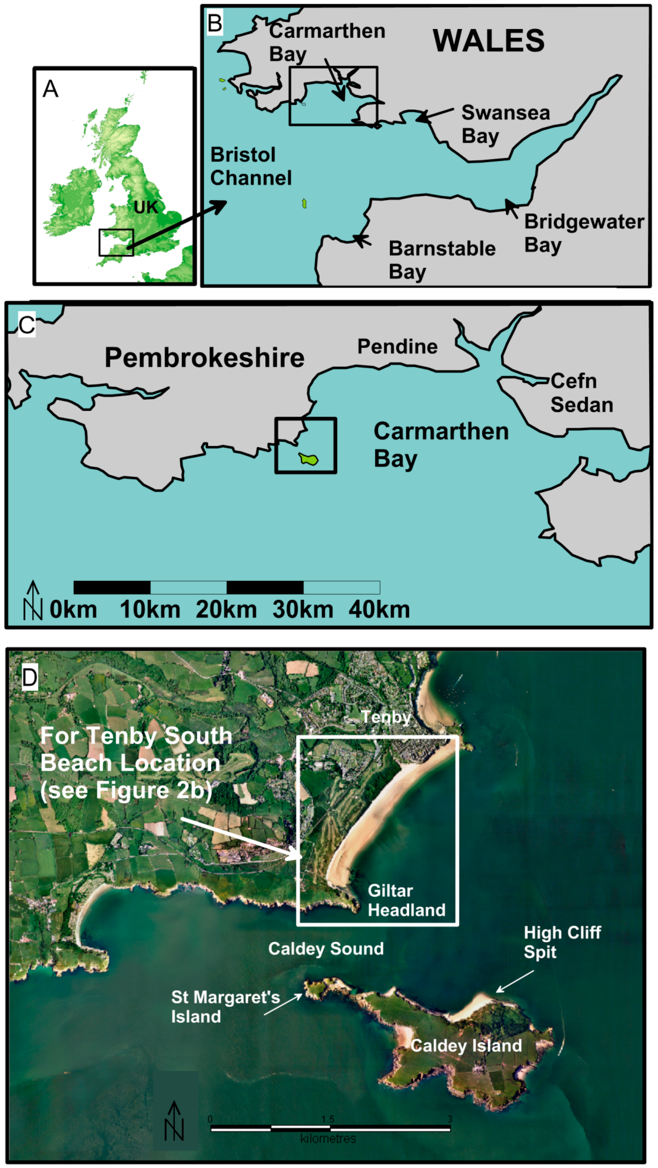
The Bristol Channel on the West coast of The United Kingdom (Figure 1A) separates Wales from Southwest England. There are a number of large embayments along the margins of the outer Bristol Channel (Figure 1B), Barnstaple, Bridgewater, Swansea and Carmarthen. Carmarthen Bay is a long sweeping embayment (30 km), described by [16] as displaying highly curved geometry (Figure 1C). Tenby Peninsula, on the western side of the bay (Figure 1C), is characterized mainly by rocky cliffs and small embayments that contain pocket beaches formed as a consequence of erosion of the softer mudstone rich Carboniferous Coal Measures and Millstone Grit [34].

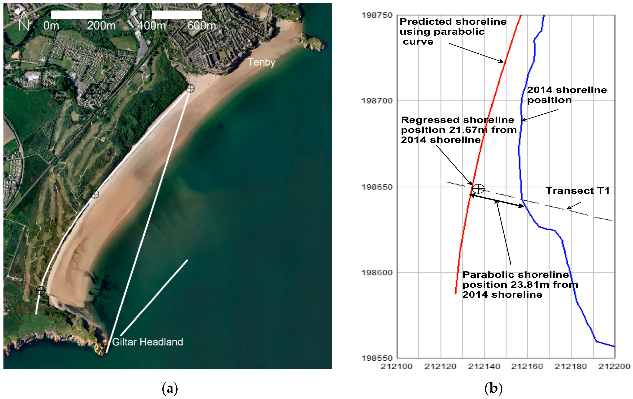
The study area (51°39′36′′ N; –4°42′36′′ W) is located between two Carboniferous Limestone headlands, Giltar to the south and Tenby to the north [35], the distance between headlands being approximately 2 km. The embayment profile is shallow and concave, with a wide (circa 250 m) sandy intertidal zone. This gives way to a limestone shingle backshore overlain by a dune system (920 × 10³ m²; [27]), shingle is periodically exposed during storms and high spring tides, and extensive vegetation retards sediment movement from the dune field to the intertidal zone. The seaside town of Tenby to the north is a heavily urbanized coastal area, where tourist activity strongly supports the regional economy. To the south, the dunes, marshes and Giltar Headland promontory are ecologically important conservation areas. Semi-diurnal and macrotidal, the region has a mean spring tidal range of 7.5 m [28], with a Mean High Water Spring Tide level (MHWST) of 5 m Above Ordnance Datum (AOD). Incident offshore waves generally approach from the southwest with an average wave height of circa 1.2 m and associated mean periods of 5.2 s [27]. Storm waves of 7 m, with periods of 9.3 s, constitute less than 5% of the wave record. Longshore drift from south to north is influenced by heavily refracted southwesterly Atlantic swell waves which undergo diffraction as they encounter the south Pembrokeshire coast and offshore islands (Caldey and St Margaret’s; Figure 1D). Between November 2013 and March 2014, a total of 32 storms (average h_s > 3.4 m) were recorded generating average waves that reached 4.7 ± 1.26 m with associated periods of 7.9 ± 1.00 s, and some waves reaching 9.3 m with periods of 12 s. These events caused widespread erosion and structural damage along the Pembrokeshire coastline.

3. Methods

3.1. Shoreline Change Modelling (1941–2014)

This paper builds upon Thomas et al.’s [27] centurial work, by utilizing additional recent data to assess morphological change between 1941 and 2014. Sixteen aerial photographs (1941–2014; Figure 2a), all geo-rectified in a Geographic Information System (Mapinfo^®, Pitney Bowes Sofware Inc, New York, NY, USA) to the British grid reference system, were used to extract shoreline position. The figures vary, some incorporate a narrow aerial extent versus a wider aerial extent. Errors in aerial photographs can be of the order of 7.5 m–8.9 m caused by distortion and the digitizing process itself [36,37]. In this paper, the former was mitigated using 600 dpi images and the latter assessed for accuracy using Root Mean Square Error (RMSE) (see [38] for theoretical interpretations and [27,39,40] for practical applications). Survey control points (Figure 2b) established using RTK Network GPS 1200+ with an average of 200 readings taken at every control point ensured accuracy. Subsequently, RMSE was calculated using RMSE = [(∑(N_c –N_t)² + ∑(E_c –E_t)²)/n]^1/2, where; N_t and E_t are calculated co-ordinates from the photo transformation, N_c and E_c are control coordinates and n is the total number of data points.

Table 1. Aerial photographic source document scales and RMSE results after digitizing.

Year	Type	Source	RMSE	Scale
1941	Aerial Photograph	Welsh Assembly	1.5	1:10,000
1946	Aerial Photograph	Welsh Assembly	2.4	1:10,000
1960	Aerial Photograph	Welsh Assembly	1.9	1:10,000
1966	Aerial Photograph	Welsh Assembly	1.6	1:10,000
1970	Aerial Photograph	Welsh Assembly	1.1	1:10,000
1978	Aerial Photograph	Welsh Assembly	1.5	1:10,000
1981	Aerial Photograph	Welsh Assembly	1.2	1:10,000
1983	Aerial Photograph	Welsh Assembly	1.3	1:10,000
1985	Aerial Photograph	Welsh Assembly	2.2	1:10,000
1989	Aerial Photograph	Welsh Assembly	1.5	1:10,000
1994	Aerial Photograph	Welsh Assembly	0.9	Digitised 40 cm resolution
2000	Aerial Photograph	Getmapping	2.4	Digitised 40 cm resolution
2006	Aerial Photograph	Ordnance Survey	1.5	Digitised 40 cm resolution
2010	Aerial Photograph	Welsh Assembly	1.5	Digitised 40 cm resolution
2014	Aerial Photograph	Welsh Assembly	1.5	Digitised 40 cm resolution

shows respective source document scales and RMSE values. The average RMSE error for the aerial photographs was 1.76 m. The vegetation line was chosen as shoreline change indicator, as this could be easily identified on all aerial photographs and is valuable for investigating long term trends [33]. The corresponding extracted shoreline position was imported into the Regional Morphological Analysis Programme (RMAP; see [41]) a module within the Coastal Engineering Design and Analysis System (CEDAS), where inter-survey and cumulative shoreline changes were evaluated. Temporal change together with rotation analysis was achieved using the 1941 shoreline position as a proxy baseline. The shoreline positions measured from aerial photographs were extracted along 12 theoretical transects (T1–T12), spaced approximately 150 m apart (Figure 2c). Linear regression and correlation analysis within the dataset constituted of the 12 shoreline signals were used to characterize the shoreline planform evolution.

3.2. Wind and Wave Data Characterization

Constant beach profile and plan-form reshaping is caused primarily by incident wave characteristics, i.e., height, period, and particularly direction. These determine wave induced sediment transport both in onshore/offshore and alongshore directions [1,2,3]. Waves and their directional components are used as direct input into coastal engineering or coastal zone management calculations [30]. However, wind is the underlying cause of most sources of coastal flood and erosion risk but wind data is rarely used in these calculations [5]. Within the region of study, synthesized wind and wave time series from meteorological numerical models that were suitable to be inputted into wave prediction models have only recently been made available. However, wind speed and directional data from the early 1940s were available and obtained from the UK Meteorological Office, enabling direct comparisons to be made between shoreline change and these environmental forcing agents. Offshore wind speed and direction data was captured at approximately 3-h intervals at a point southeast of the study area (51°24′00′′ N; −5°00′00′ W). Some of the early data was missing but, nevertheless, the dataset contained circa 147,000 independent values.

Based on calculated storm wave statistics from south-easterly, southerly and south-westerly directions, storm wave statistics were characterized using significant wave height, period and direction. Data was captured at 1 h intervals between 1998 and 2013 from a waverider buoy located southwest of the study location (NOAA station number 62303; 51°36’00’’ N; 4°34’48’’ W). Subsequently, wave energy, alongside storm frequency, power and class were computed using the methodologies of [40,41,42,43,44,45,46,47], with a detailed discussion and practical use given by [5] and, in all, a total of 267 storm events were identified during the assessed 15-year period. This approach differs from that adopted by [42] and [43] within the same study region as they used a minimum wave height of 1.5 m when characterizing waves that were capable of imposing morphological change at Tenby and nearby Pendine and Cefn Sedan, respectively (Figure 1C). The storm climate waves used in this research were characterized using a minimum wave height of 3.4 m (i.e., Hs ≥ 3.4m) because they represented rare events in Carmarthen Bay only occurring 8% of the 15-year period recorded.

Wave data were subsequently modeled using the Regional Coastal Processes WAVE propagation model (RCPWAVE), a module within the Nearshore Evolution MOdelling System (NEMOS), which forms an integral part of the Coastal Engineering Design & Analysis System (CEDAS 4.03, Veritech Enterprises, Arlington, MA, USA). RCPWAVE is a two-dimensional steady-state and modified form of the “mild slope” equation for monochromatic waves and simulates linear plane wave propagation over arbitrary bathymetry. Originally developed by [44] and documented by [45], the model considers shoaling, refractive and bottom-induced diffractive effects outside the surf zone where wave reflection and energy losses are considered negligible. The wave model grid offshore boundaries were generated using the GRId GENeration (GRIDGEN) module within NEMOS. The offshore model boundary was restricted to the 26 m isobath, as this was the optimum depth at which the Meteorological Office originally computed wave height, period and directional components. A rectangular computational grid of 10 m × 10 m square mesh that encompasses the coastal region was then used to predict wave conditions at Mean High Water Spring Tide (MHWST) wave conditions. The established wave direction vectors were subsequently used to assess sediment pathways fronting South Sands.

3.3. Equilibrium Model

To predict shoreline equilibrium, data were input into an empirical formulae based upon the Parabolic Bay Shape Equation (PBSE) developed by [46] and [47]. In their manual application, a vertical aerial photograph is used to obtain the main model variables (β and R₀; Figure 3) for input into the equation. R₀/R_n = C₀ + C₁ (β/θ) + C₂ (β/θ) ². In the case of a single up-coast headland, the distance R₀, i.e., the length of a control line drawn from the end of the headland to the nearest point on the down-coast shoreline where the shoreline is parallel with the predominant wave crest, is estimated directly from the aerial photograph. In this research, the distance from the headland to the downcoast control point (R₀) and wave approach angle (β) was estimated by predicting the zero migration date from a linear regression trend. The established date is then used to extrapolate both northern shoreline position and the region of rotation, once again based upon linear regression trends. The angle β (30°) was sub-tended between a line joining the predicted region of rotation and northern shoreline position and the control line R₀ (1357 m). The distance R_n, measured from the end of the up-coast headland defines the shoreline location at a varying angle θ. The coefficients C_o (0.045), C₁ (1.146) and C₂ (−1.94) were derived from the seminal workings of [46] and [47]. Finally, a GPS topographic survey was performed to establish ground levels along the predicted southern shoreline position in order to assess both flood vulnerability to imposed morphological change.

4. Results

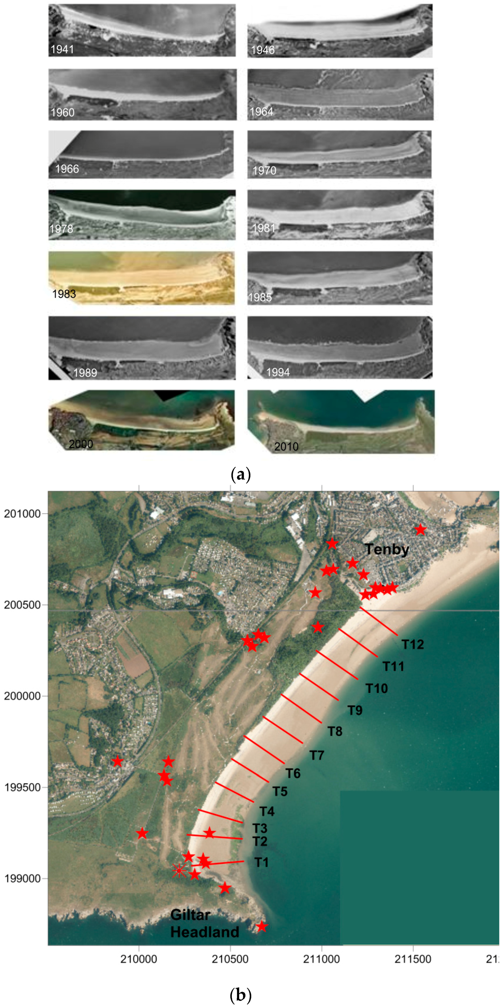
The following qualitative and quantitative assessment of 2 km of shoreline using aerial photographic evidence provides an illustration of shoreline changes from 1941 to 2014.

4.1. Temporal Change (1941–2014)

Once the aerial photographs were geo-referenced, shoreline positions were extracted (Figure 4). The southern shoreline retreated consistently throughout the assessment. Two concrete groynes were constructed in the 1930s to protect a shooting range sited within the southern dune system, but their design caused downdrift erosion and arguably augmented recession rates. The shooting range was eventually relocated landward of the dune system and the groynes were eventually demolished in the early 1990s. All that remains of the original shooting range are partially collapsed butts (Figure 4 beach sector a). The shoreline now evolves naturally taking a typical embayed shape. Crucially, the construction of a gabion wall in the early 1980s has arguably prevented shoreline retreat (Figure 4 beach sector b). However, the structure was also outflanked and its presence caused downdrift erosion that exposed a large blow out to direct wave attack. The gabion wall was destroyed and the blow out collapsed during the 2013/2014 winter storms. Part of the gabion wall was reconstructed and the dune system around the blow out is already showing signs of recovery. The shoreline change trends within this sector changed from erosive to accretive resulting from additional sediment input from the 20 m high blow out. Apart from the 1960 shoreline that appeared to be erroded, the northern sector showed gradual accretion throughout the assessed period (Figure 4 beach sector c).

Table 2. Shoreline position by transect, in relation to the 1941 baseline (Note: negative values depict shoreline retreat, positive values depict shoreline advance and all values are in meters).

Timescale (Years)	Oscillation Point	T1	T2	T3	T4	T5	T6	T7	T8	T9	T10	T11	T12	Average T1-T4	Average T5-T8	Average T9-T12
1941		0	0	0	0	0	0	0	0	0	0	0	0	0	0	0
1946	630.5	−3	−9	−14	−14	2	2	22	24	−1	0	7	4	−10	13	3
1960	780.9	2	−19	−25	−27	−7	0	16	18	−1	4	−3	6	−17	7	1
1964	804.8	−10	−23	−36	−34	−12	3	21	24	4	1	1	14	−26	9	5
1966	796.5	−9	−22	−36	−36	−13	4	24	27	5	2	0	12	−26	11	5
1970	818.6	−19	−19	−36	−36	−16	3	26	26	5	4	2	13	−27	10	6
1978	841.4	−33	−20	−38	−37	−25	0	26	26	5	2	4	14	−32	7	6
1981	874.7	−37	−22	−40	−40	−28	−3	23	26	6	0	1	9	−35	5	4
1983	861.5	−37	−21	−39	−36	−27	−3	26	28	9	2	3	13	−33	6	7
1985	885.8	−36	−26	−40	−37	−25	−5	23	24	5	−2	−2	6	−34	4	2
1989	856.7	−40	−28	−40	−37	−26	−4	28	32	12	7	7	16	−36	7	10
1994	873.2	−45	−32	−42	−39	−26	−15	27	31	13	4	7	16	−39	4	10
2000	911.7	−53	−39	−41	−38	−23	−20	26	27	23	16	9	17	−43	2	16
2006	864	−53	−43	−40	−39	−28	−13	19	35	21	12	17	18	−43	3	17
2010	978.8	−54	−48	−45	−42	31	−25	−1	10	18	10	13	14	−47	4	14
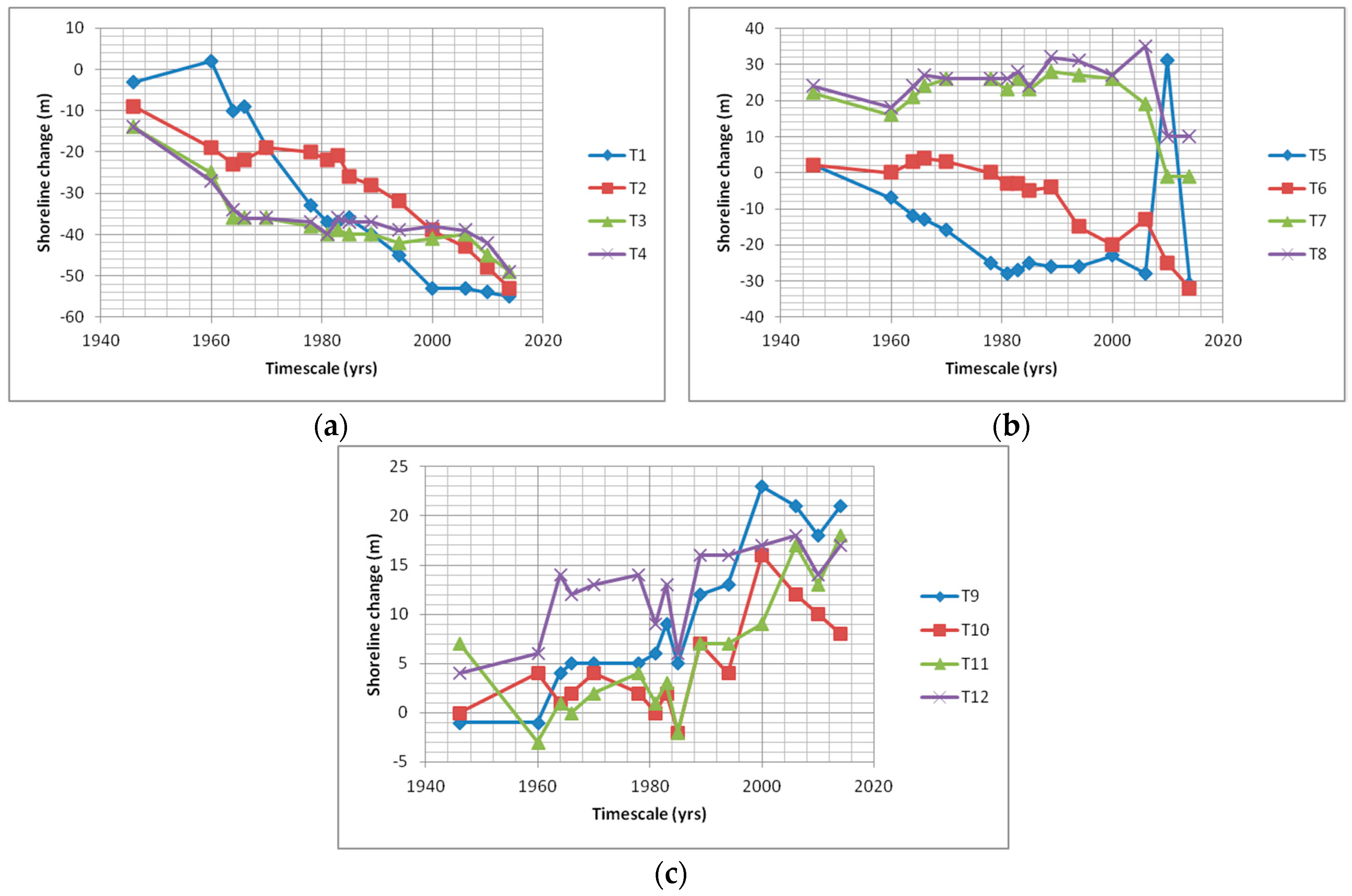
2014	978.8	−55	−53	−49	−49	−31	−32	−1	10	21	8	18	17	−52	−14	16

was constructed by direct measurements of the shoreline position along each transect presented in Figure 2b compared to the 1941 baseline. Timeseries show a landward excursion of the southern shore with an average overall loss of 55 m (T1–T4; Figure 5a), in the central sector, the southernmost transects (T5–T6) eroded by circa 31m and the northernmost accreted by circa 10 m (T8; Figure 5b), the shoreline at T7 remained stable (−1 m). In contrast to the south, northern shores accreted albeit with more variation through time resulting in an average overall gain of 16 m (T9–T12; Figure 5c).

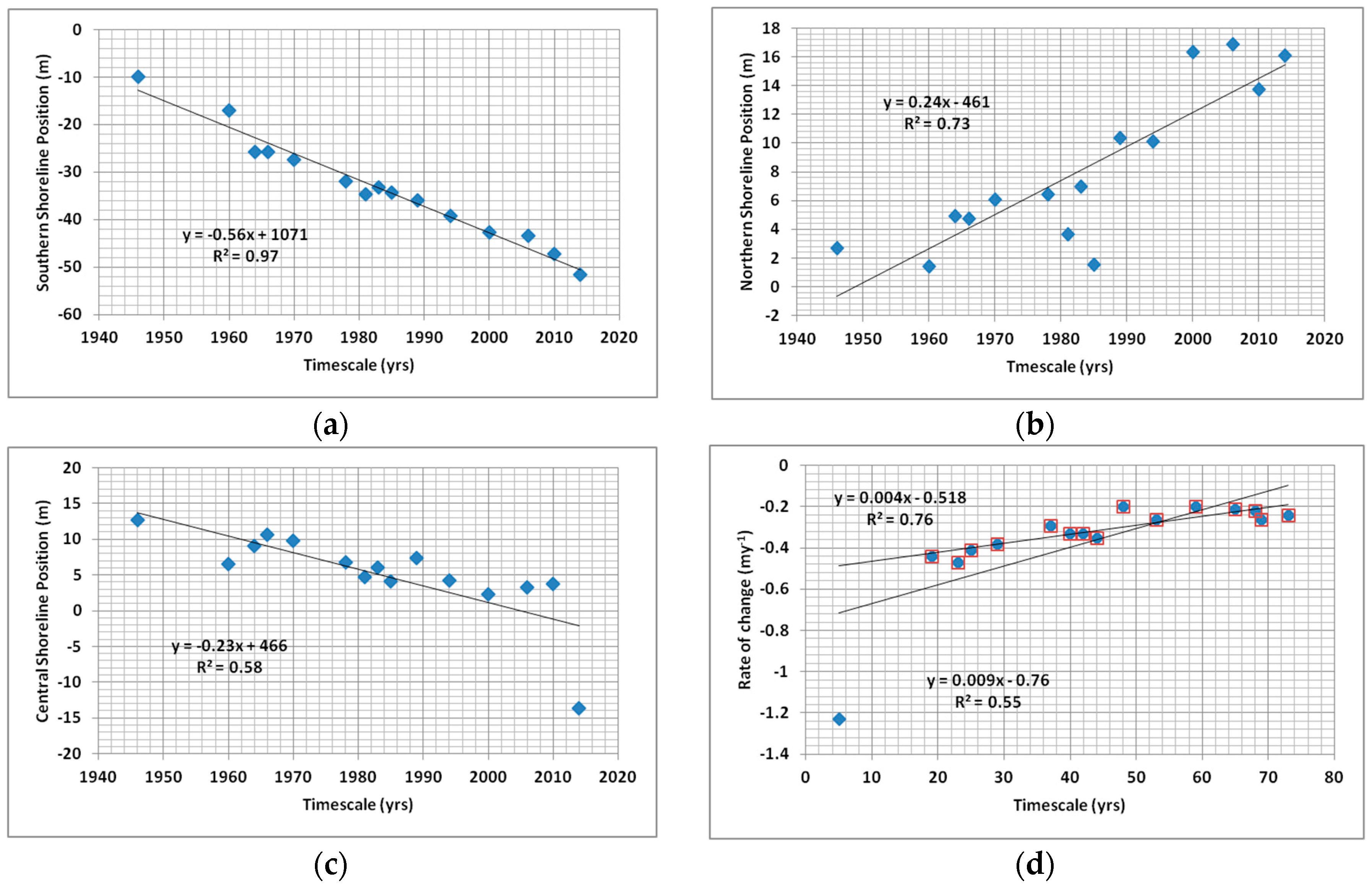
An assessment of temporal changes showed high correlation indicating a consistent trend of southern shoreline erosion given by the regression equation y = −0.56x + 1071, while the regression model coefficient of determination (R² = 97%) showed that a significant percentage of spatial variation was explained by a constant migration rate (p < 0.01; Figure 6a). With lower correlation, northern shores accreted and the regression equation y = 0.24x − 461 (R² = 73%) showed that a high percentage of spatial variation could be explained by a constant migration rate (p < 0.01; Figure 6b). Similar to the southern sector the central sector shoreline also eroded (y = −0.23x + 466) and even though the R² value explained just over half of the spatial variation through time (R² = 58%), results were still statistically significant at the 95% confidence level (Figure 6c).

RMAP was utilized to compute the cumulative change rates shown in

Table 3. The shoreline change rate record. (Note: negative values depict shoreline retreat, positive values depict shoreline advance and all values are in meters).

Timescale		Time Span from 1941 Baseline	Inter-survey Change Rate m·year−1	Cumulative Change Rate m·Year−1
From	To
1941	1946	5	−1.23	−1.23
1946	1960	19	−0.12	−0.44
1960	1964	23	−0.50	−0.47
1964	1966	25	0.04	−0.41
1966	1970	29	−0.16	−0.38
1970	1978	37	0.05	−0.29
1978	1981	40	−0.95	−0.33
1981	1983	42	−0.28	−0.33
1983	1985	44	−0.73	−0.35
1985	1989	48	0.90	−0.2
1989	1994	53	−0.85	−0.26
1994	2000	59	0.32	−0.2
2000	2006	65	−0.22	−0.21
2006	2010	69	−0.50	−0.26
2010	2014	73	0.12	−0.24

. The programme compares respective shoreline positions against a predetermined landward baseline at 10 m intervals along the beach frontage.

A regression model constructed using Table 3 cumulative data showed that a statistically high positive correlation and marked relationship existed (Figure 6d). The regression model demonstrated that between 1941 and 2014, a linear trend explained over half of the overall shoreline rates of change. (R² = 55%; p < 0.01) and suggested that there was a reduction in shoreline retreat through time. Observed rates of change between 1941 and 1946 are substantial in relation to all other values. Therefore, a regression model was constructed with this value removed, once again highlighting with a very high positive correlation that a linear trend could explain a significantly high percentage in overall shoreline rates of change (R² = 76%; p < 0.01). This indicates continued shoreline retreat, decreasing in severity over time. The results were heavily influenced by the initial shoreline response to the construction of the groynes in the southern sector.

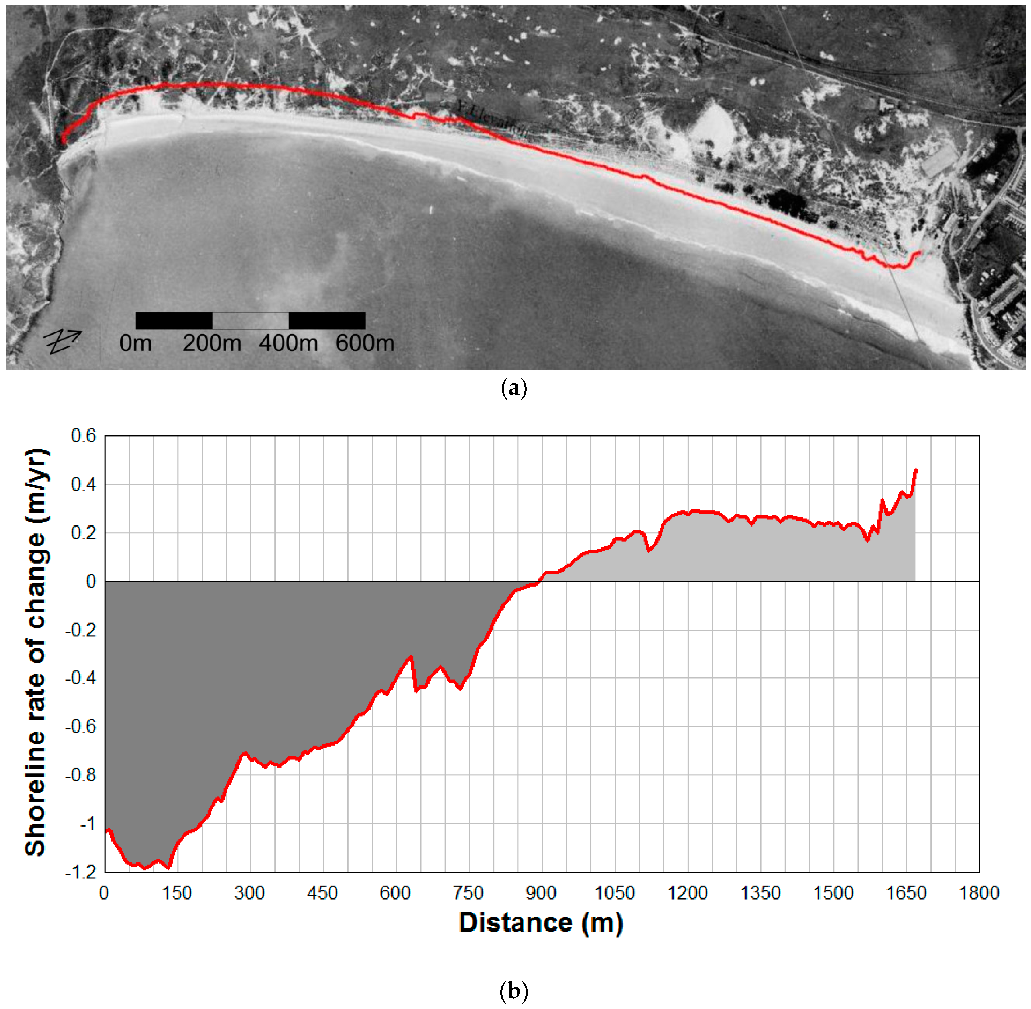
The 2014 vegetation shoreline indicator, delineated by a solid red line, was superimposed upon the 1941 aerial photograph (Figure 7a) and highlights the significant erosive trend in the southern beach sector, central stability and northern advance throughout the assessment period. Overall shoreline rates of change between 1941 and 2014 (Figure 7b) confirmed previous trends showing that southern shores retreated at a maximum rate of 1.18 m/year, contrasting against a maximum northerly advance of 0.4 m/year. The rotation point was observed near the beach centre at circa 850 m alongshore from Giltar Headland. Overall, the frontage of South Beach showed a recession trend (circa 18 m; Table 3) throughout the 73-year period.

4.2. Assessment of Beach Rotation (1941–2014)

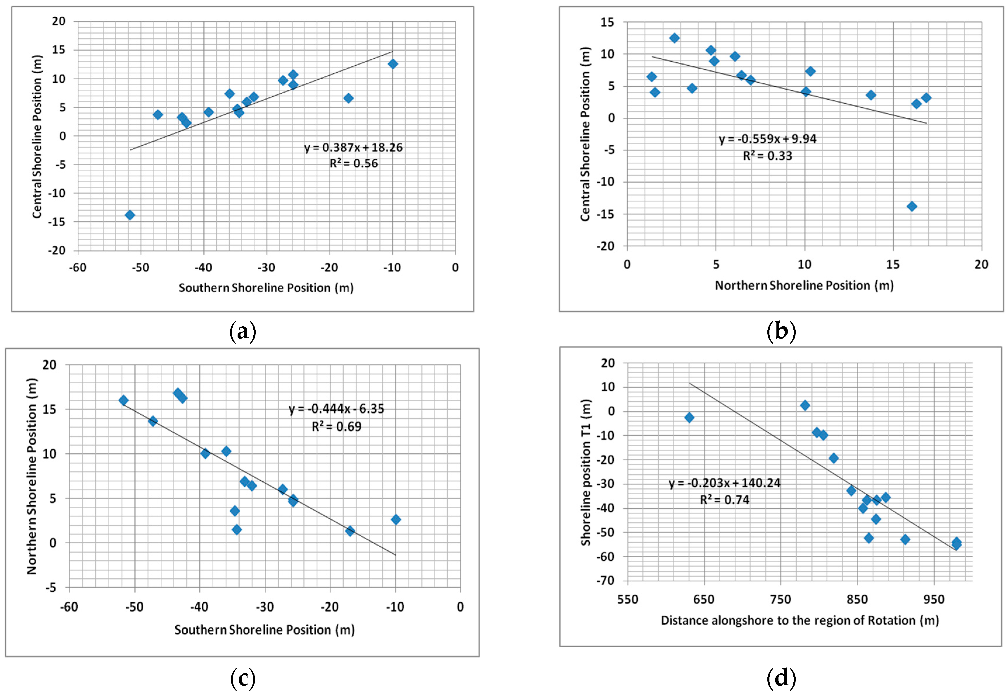
A positive relationship existed between southern and central sectors given by the regression equation y = 0.387x + 18.26 and coefficient of determination (R²) that explained 56% of data variation (p < 0.01; Figure 8a). Results indicated that when changes occur in the southern sector, they also occur in the central sector. In contrast, a negative phase relationship existed between northern and central sector cross-shore positions y = 0.587x + 9.94 (R² = 33%, p < 0.05; Figure 8b), indicating that when changes take place within the northern sector the opposite would be true in the central sector. However, it is the statistically high negative phase relationship that existed between southern and northern beach extremities, given by the regression equation y = 0.444x − 6.35 explaining 69% of data variation (p < 0.01; Figure 8c), that is of most interest, as this indicates that beach rotation exists. A statistically high relationship also existed between the steady migration northward of the observed point of rotation and southern shoreline changes, given by the regression equation y = 0.203x + 140 that explained 74% of data variation (p < 0.01; Figure 8d).

Table 4. Pearson correlation coefficients set at zero timelag compare longshore inter-survey shoreline positions by transect 1941–2014. Note: bold, p < 0.05, bold italic, p < 0.01 and grey area highlights the negative relationships involved in the rotation process.

T2	0.84
T3	0.82	0.77
T4	0.76	0.76	0.98
T5	0.28	0.04	0.32	0.33
T6	0.84	0.94	0.66	0.64	0.02
T7	0.22	0.56	0.26	0.34	−0.49	0.56
T8	−0.11	0.17	0.04	0.12	−0.56	0.25	0.86
T9	−0.90	−0.92	−0.73	−0.68	−0.19	−0.88	−0.27	0.10
T10	−0.66	−0.76	−0.44	−0.41	−0.06	−0.73	−0.13	0.20	0.86
T11	−0.74	−0.82	−0.45	−0.42	−0.07	−0.82	−0.38	0.05	0.85	0.78
T12	−0.70	−0.72	−0.74	−0.70	−0.30	−0.59	−0.07	0.25	0.83	0.71	0.69
	T1	T2	T3	T4	T5	T6	T7	T8	T9	T10	T11

produced from Table 2 (Columns 3–14) shows a Pearson correlation matrix constructed to compare the temporal variation along each profile from the 1941 baseline. Positive high correlations signify that substantial relationships existed between southern profiles (T1–T4), indicating that when changes occur at one profile location they also occur on adjacent profiles (p < 0.01). A similar scenario existed within northern profiles (T8–T12) where positive correlations, varied between moderate and high. With the exception of the correlation between T8, all results were significant at 95% or 99% confidence (p < 0.05–p < 0.01; Table 3). The central profiles (T5–T8) showed statistically insignificant positive/negative correlations that varied from negligible to moderate (p > 0.05).With the exception of positive/negative high correlations between T6 and the southern/northern profiles, insignificant correlation existed between remaining central profiles and both southern and northern profile locations.

However, it is the statistically high and very high negative correlations that are of most interest as they signified marked and very dependable inverse relationships between north and south sectors i.e., beach rotation (T1–T4 and T8–T12) statistically significant at the 95% or 99% confidence (p < 0.05–p < 0.01) confirming earlier regression model results (Figure 6). Negative correlation was also observed between the south and central sector. Coincidently, this also concurs with results shown by both [11] and [19] in studies of long-term rotational trends at Narabeen Beach, Australia. The fulcrum is observed at the change of correlation signs within the central region, and finds agreement with the work of [16] along the Brazilian coastline and [27] in the present region of study.

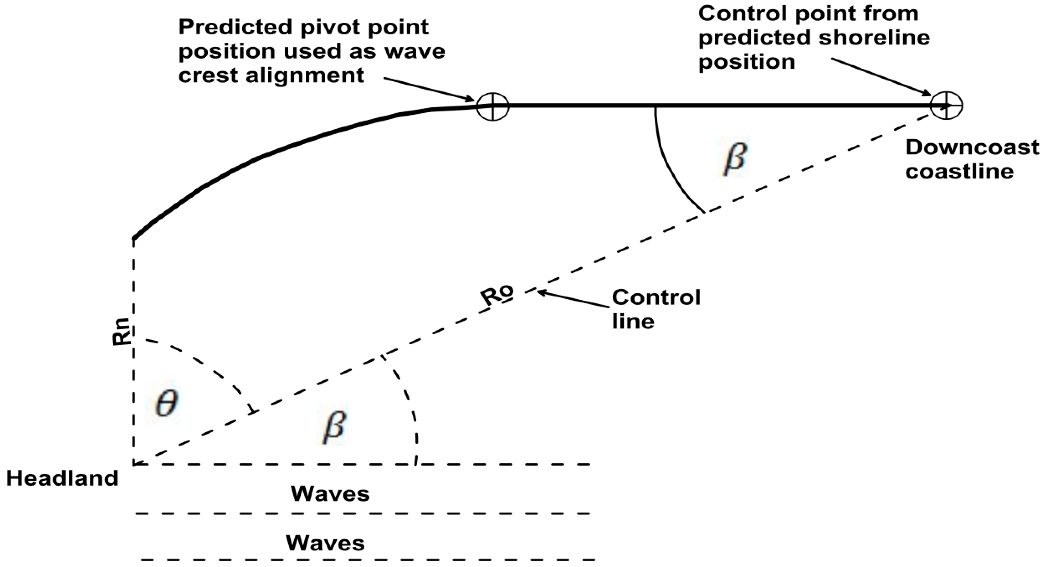
4.3. Shoreline Position Forecast

The equilibrium bay shape equation developed by [46,47] was used to estimate the expected shoreline position corresponding to a zero migration rate. The zero migration date (Z_mr) was extrapolated from the linear trend obtained in Figure 6d and given by Equation (1). The date was then inputted into the linear trends obtained for southern (S_sp) and northern (N_sp) shorelines (Figure 6a,b respectively) and 2061 shoreline positions computed (Equations (2) and (3)). The extrapolated southern shoreline position was inputted into the linear trend obtained for the region of rotation (Figure 8d) and the region of rotation (C_rr) computed (Equation (4)). To estimate the predominant wave direction a perpendicular line was drawn from the predicted northern shoreline position (i.e., downcoast control point) to the predicted point of rotation. Figure 9b shows the southern shoreline sector, highlighting the 2061 shoreline position extrapolated from the linear trend obtained from Figure 6a (black cross within a circle) and the predicted bay shape using the 2nd order parabolic curve (red line) alongside the 2014 shoreline position (blue line). Results show the efficiency of using both linear trends and empircal bay shape equations.

Z_mr = [(0.5086/0.0044) + 1946] = 2061

(1)

S_sp = -0.56 (2061) + 1071 = −83.16 m (from 1946 baseline)

(2)

N_sp = 0.24 (2016) − 461 = 33.64 m ( from 1946 baseline)

(3)

C_rr = [-(−83.16) +140.24)]/−0.203 = 1100.498 m (from T1)

(4)

4.4. Wave Models

In this region, extreme storm waves (>3.4 m) make up 6% of the record and expose the coast to waves and associated periods that can reach 7 m and 9.3 s, respectively. However, these storms are rare with on average of two occurrences a year. The majority of storm waves (circa 90% of the record) range between 4.7 m and 6.5 m with associated periods of 8 s to 8.6 s. Offshore Island location, bathymetry, Bristol Channel fetch limitation and the orientation of the shoreline narrows the range of wave directions experienced at frontage of South Beach. This was shown in the extreme wave results of both [42] and [43] who highlighted similar regional patterns of wave directional change irrespective of wave height and period variation (i.e., 1:1 month, 1:1 year and 1:10 year assimilations). This present paper used extreme storm events from the same assessed directions (southwest, south and southeast); modelled vectors were once again similar irrespective of the event severity. 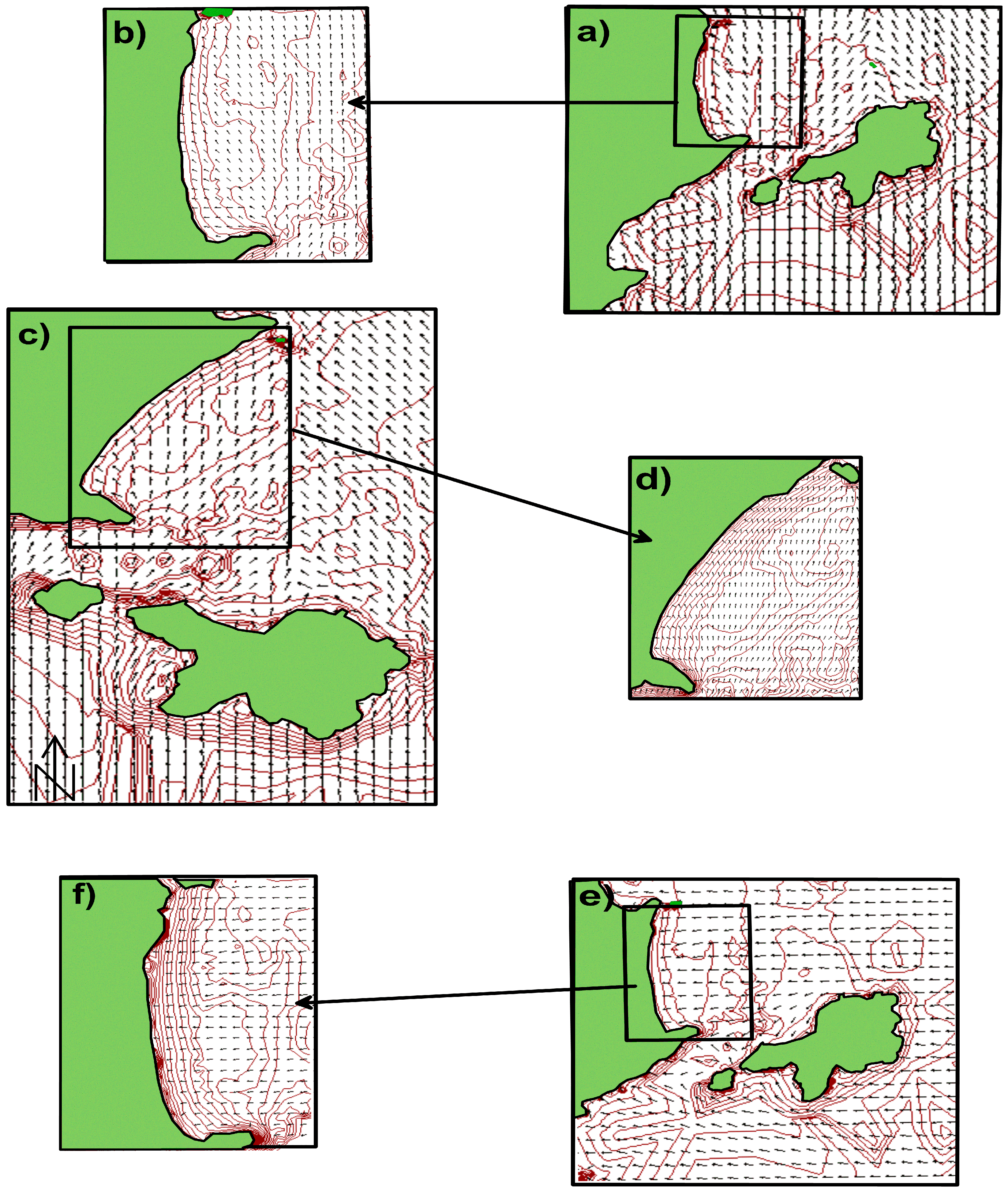Therefore, Figure 10 only shows simulation of the most extreme storm waves encountered in each of the assessed directions. Southwesterly waves are heavily diffracted around St Margaret’s Island before entering Caldey Sound and impact Giltar Headland at an acute angle, where further diffraction takes place as waves enter South Sands littoral (Figure 10a). Wave energy is focused at an obtuse angle to the beach (Figure 10b), suggesting a northward sediment pathway (Tenby). Under southerly conditions generated waves are heavily diffracted around both Caldey and St Margaret’s Islands before entering South Bay. The two wave trains meet and form a shadow zone along the trace of High Cliff spit (Figure 10c). It is reasonable to deduce that through wave energy loss; entrained sediments derived from Caldey Sound would be deposited explaining both continued sand spit growth and sediment loss in Caldey Sound reported by [29]. Further refraction once again refocuses waves at an angle along the frontage of South Beach. Therefore, it is also reasonable to deduce that southerly waves would be the cause of south toward north longshore drift (Figure 10d). In contrast, southeasterly waves diffract around the easternmost point of Caldey and on entering South Bay, become parallel to the island frontage. This has the effect of reducing wave impacts generated within Caldey Sound from St Margaret’s Island (Figure 10e). These waves approach South Beach at a slight southward angle (toward Giltar Headland), and under these conditions, longshore sediment pathways would emanate (albeit weakly) from Tenby towards Giltar Headland (Figure 10f).

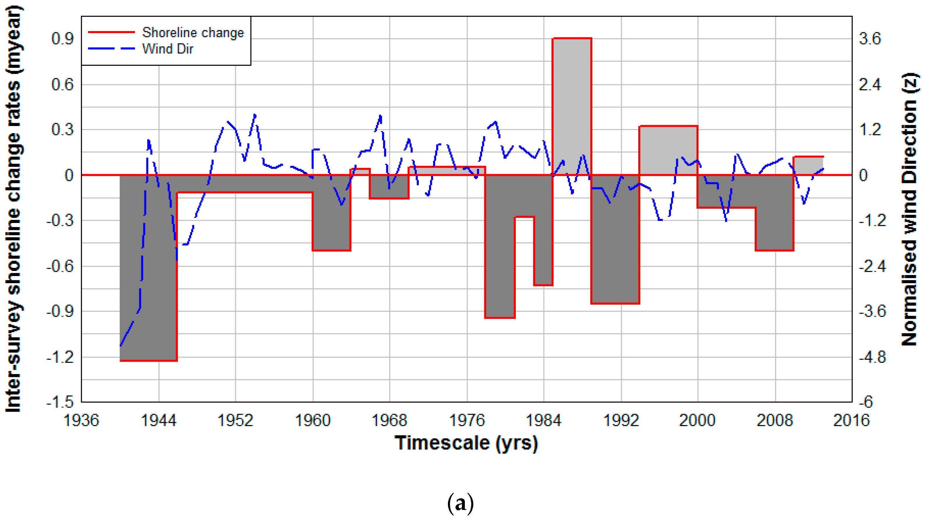
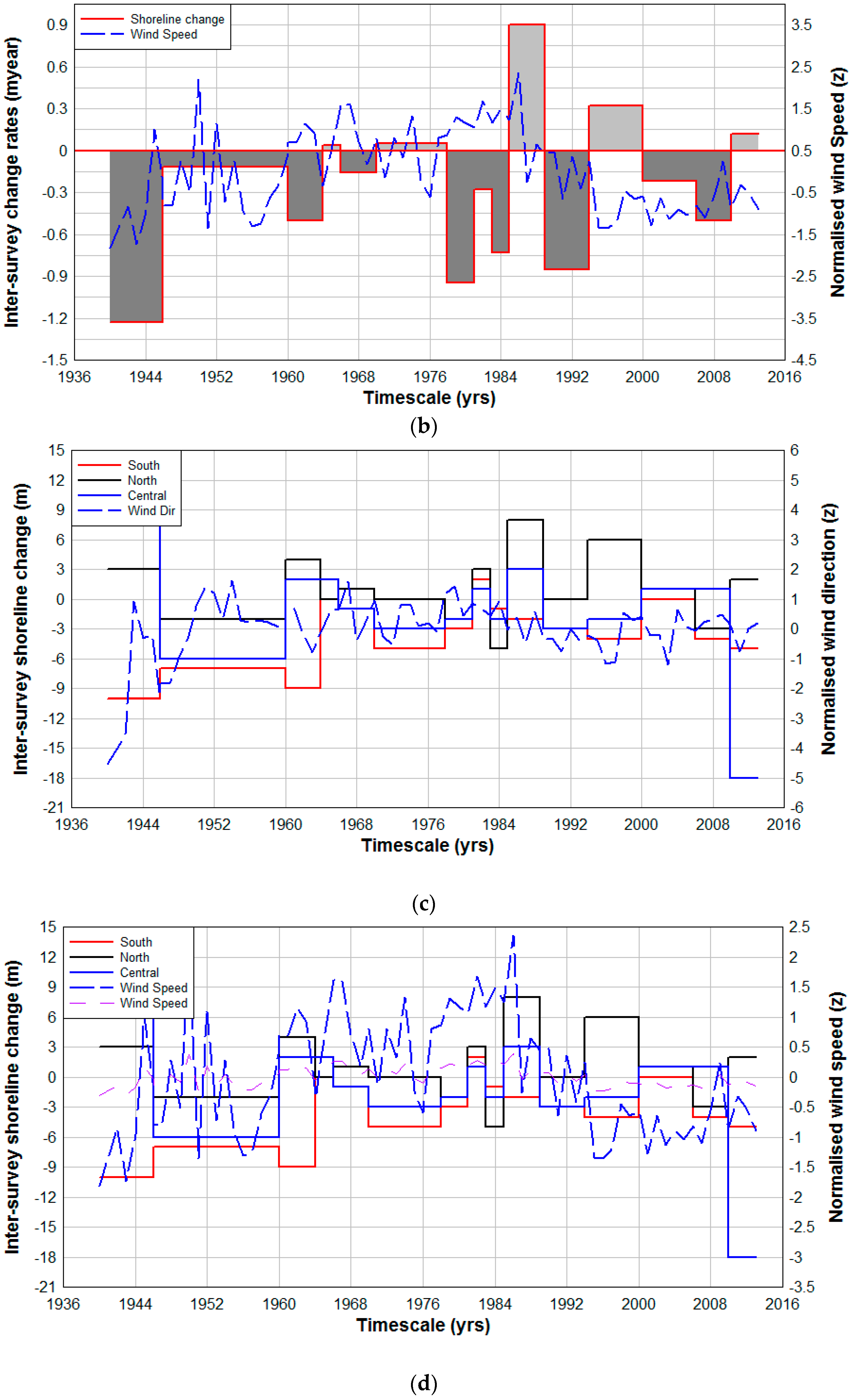
4.5. Shoreline Changes in Relation to Wind Conditions

Within the region of study, synthesized wind and wave timeseries from meteorological numerical models suitable to be used in qualitative and quantitative assessments have only been available since 1986. However, comprehensive sets of wind speed and directional data were available from the early 1940s and used to assess shoreline behavior against these imposed environmental forcing agents over an historic timeframe.

The largest landward excursion of the shoreline (Table 3) took place between 1941 and 1946 (−1.23 m/year) and occurred when both direction (0 = 206 ± 16.9°, Figure 11a) and wind speed (0 = 7 ± 0.97 m/s; Figure 11b) are below average, suggesting that winds predominate from south toward east, with a wind speed reduction as a consequence of the limiting Bristol Channel fetch. A reduction in shoreline retreat rates was observed between 1946 and 1960 (−0.12m/year), as winds predominated from a southeasterly direction (negative) in the early 1950s shifted to a southwesterly one towards the middle of the decade returning to a mean direction of around 210° at the end. The highest winds during this timeframe also occurred during the early 1950s followed by a period of below average wind speeds. Increasing wind speeds, as wind direction fluctuates above and below the average value, corresponded to a landward shoreline excursion (−0.5 m/year) between 1960 and 1964. Observed changes 1964–1966 and 1970–1978 indicated shoreline advances albeit small, which reversed the more general trend (0.04 m/year and 0.05 m/year, respectively); wind speed and direction fluctuated between negative and positive values. Between 1966 and 1970, a shoreline retreat of −0.16 m/year occurred during a period that is dominated by increasing wind speed and winds from a southwesterly direction.

The system returned to the more normal trends of shoreline retreat 1978–1981, 1981–1983 and 1983–1985 (−0.95 m/year, −0.28 m/year and −0.73 m/year, respectively). Once again, southwesterly winds and rising wind speeds dominated this period. Apart from high speed in 1984, wind speed trend is near and below the average value, and the direction was predominantly from the southeast to south during two periods of shoreline advance of 0.9 m/year and 0.32 m year (1985–1989 and 1994–2000, respectively). However, similar trends of wind speed and direction to previous values were observed between 1989 and 1994 that resulted in a shoreline retreat of −0.85 m/year. The shoreline is observed to have retreated between 2000 and 2010 (−0.5 m/year), when winds were lower than average and wind direction fluctuated between southwest and southeast. Extreme storms were recorded between late 2013 and early 2014 that caused erosion along the southern sector, i.e., a landward excursion of the vegetation line. However, overall the frontage showed a slight increase (0.12 m/year) as the northern sector accreted. Regional wave data covering the period up until the end of 2013 showed that relatively weak wind speeds predominated, suggesting that the bulk of the erosion took place during the January/February 2014 storms.

Table 2 data was transformed to characterize inter-survey changes by beach sector (south/central/north) and compared to wind direction (Figure 11c) and wind speed (Figure 11d). The overall erosion trend highlighted in Table 2 between 1941 and 1946 was restricted to the southern sector as both central and northern sectors accreted under south/southeast (below average) and less energetic wind regimes. When southerly wind directions were encountered under a variable wind speed, there was reduction in the erosive trend within the southern sector and losses in both northern and central sectors (1946–1960). Under less energetic wind speed and directions emanating from south toward southwest, there is variable erosive/accretive behavior within all beach sectors (1960–1978). Southwesterly wind directions and variable below average wind speeds result in southern erosion, contrasted against northern accretion with central sectors varying between erosion and accretion throughout (1978–present).

5. Discussion

In times of accelerated sea level rise and increasing demands on beaches to provide defense against flood and coastal erosion, coastal practitioners need robust and “hands on” approaches that simplify beach management. This article describes a simple methodology particularly useful to embayed beach coastal management. Qualitatively, inter-survey change rates varied throughout the assessment period showing a mainly erosive trend. In the southern sector, two concrete groynes and gabion walling exacerbated erosive trends. The groynes were eventually demolished and the southern sector has evolved into a classic embayed beach shape, while the gabion walling was destroyed during the winter storms of 2013/14. Quantitatively, cumulative results showed erosive trends that reduced over time suggesting that the bay is slowly reaching equilibrium. The statistically significant (R² = 76%; p < 0.001) regression models that were constructed to assess temporal trends enabled shoreline equilibrium to be predicted (2061) but the result should be treated with caution as the linear trend used for the prediction was heavily influenced by an accelerated retreat rate between 1941 and 1946. However, this does not diminish the importance of this research that proves the principle that the developed models can be used to predict shoreline position at any given temporal epoch. For example, large-scale assessments of the UK coastline use standardized epoch timescales of 20, 50 and 100 years and these are indoctrinated in all shoreline management plans [5,32]. When the present shoreline was compared with the 1941 aerial photograph, the south shoreline eroded (max = 1.1 m/year) and the northern shore advanced (max = 0.4 m/year), while the central sector remained stable. An assessment of temporal recession/accretion rates at specific locations alongshore, highlighted statistically significant southern and central erosive trends (R² = 79% and R² = 58%; p < 0.01), northern accretive trends (R² = 73%; p < 0.01).

Regression models were once again constructed to assess beach rotation and when the central sector was compared with the south a positive phase relationship existed indicating that when changes take place in the south, similar changes take place in the central region (R² = 56%; p < 0.05). Conversely, when the central sector was compared with the north, a negative phase relationship was found suggesting that when changes occur in the central sector, the opposite would be true for the north (R² = 33%; p < 0.05). What was of most interest was the negative phase relationship that existed between the southern and northern shores suggesting that when changes take place in one sector, the opposite would be true in the other sector (i.e., beach rotation). Rotation phenomena relies upon the beach rotating about a central pivot point and the regression model representing spatial trends in southerly shoreline position, and the point of rotation quantitatively verified a temporal trend of northward migration (R² = 74%; p < 0.01). This rotation point was recognized using correlation coefficients set at zero timelag, a point of rotation was centrally placed, at which a negative phase relationship changed to positive, confirmed by increasing variability in the regression model of the central beach sector (Figure 6c). These temporal models represent shoreline indicator variation (i.e., vegetation line) and were used as a simple tool in the prediction of shoreline position at the expected time of equilibrium (i.e., 2061). Analysis using these equations suggests that southern shorelines will retreat by circa 72 m; northern shorelines will advance by circa 25 m by 2061 (from the 1946 shoreline). The parabolic bay shape equation used to predict the equilibrium shoreline position compared favorably with extrapolated linear trend results.

Paucity of environmental data (wave height, period and direction) and the temporal spacing of the aerial photographic evidence make assessment of shoreline change influences difficult. However, qualitative assessments between inter-survey overall and sectored shoreline changes, wind speed and direction data do highlight that southeasterly regimes tended to be accretive and south/southwest erosive. Storm wave model results were based upon the south, southwest predominant and southeast subdominant directions. Wave models showed similar vector alignment irrespective of wave height. Results suggested that, in addition to erosion caused by south/southwesterly winds, the dominant south/southwesterly waves produce south toward north longshore drift resulting in erosion in the southern sector and accretion in the north. On the contrary, in association with southeasterly winds related to accretive trends, sub-dominant southeasterly waves produce a counter drift, albeit weak, that is reversing the general evolution trends. Additional short term assessments of wind and wave effects on the shoreline evolution are required to confirm the qualitative assessment of the present study.

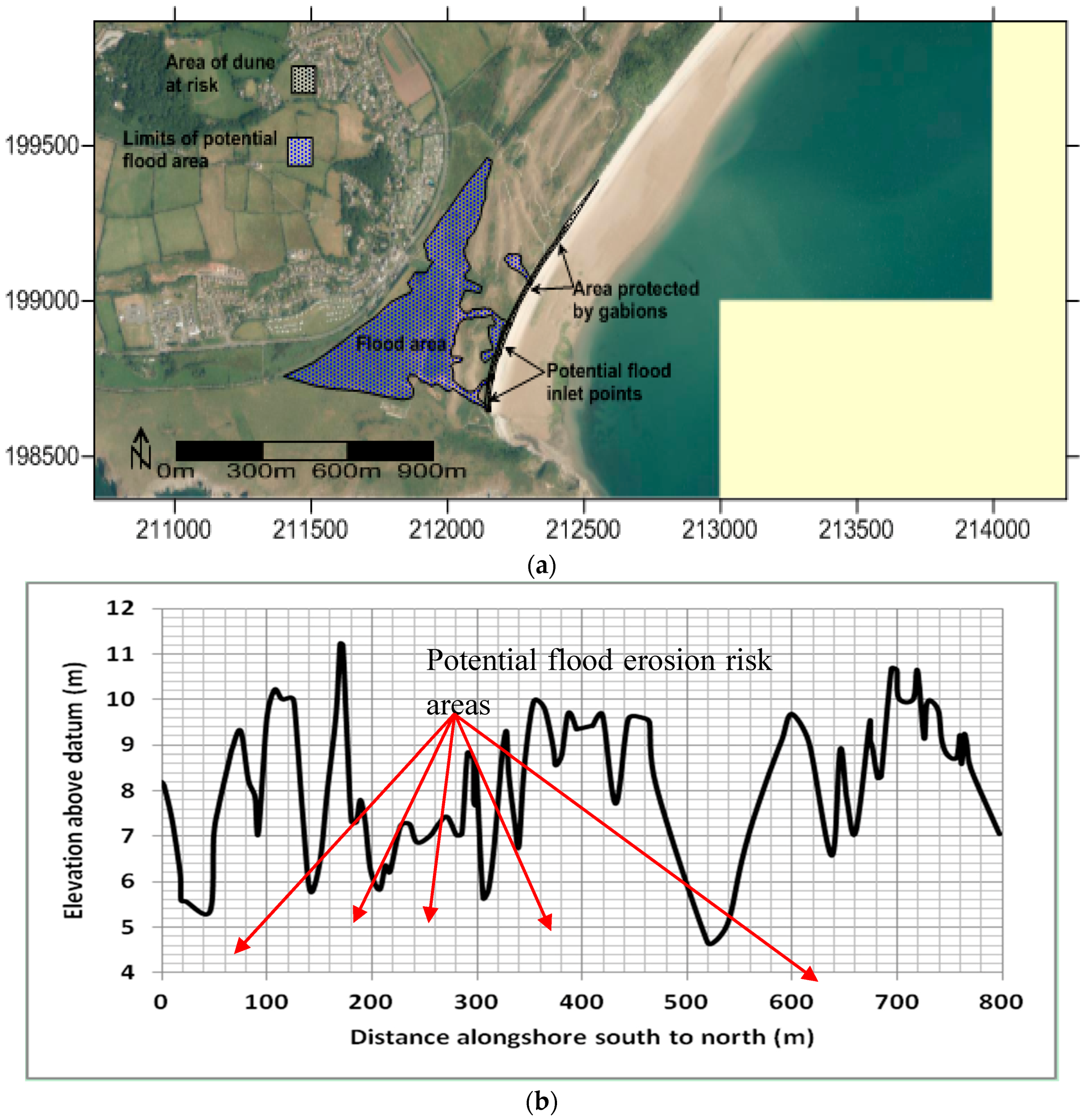
Results were used in conjunction with topographic surveys of the hinterland to produce a flood map (Figure 12a) based upon the predicted southern shoreline position (2061) and the inland 5 m contour line (i.e., the highest spring tide level). The map identified potential flood inlet points confirmed by a topographic survey along the equilibrium shoreline; one near the headland itself would allow water to access the hinterland along a low lying track, two at 100 m and 300 m alongshore along the line of a newly formed footway access to the beach and near an eroding blowout (500 m alongshore) that collapsed on the seaward side and is open to wave attack on most spring tides. The hinterland behind the dune system is already located below MHWST. A length of dune extending from the headland to the northern end of the gabion basket wall would be at risk along its entire length (circa 400 m). The area of flood potential extends from the dune field to the railway line that was constructed in an elevated position in relation to the MHWST level and would act as a barrier to further ingress. It has to be remembered that the area would only flood during the spring tidal range or during storm surge conditions. This could also be mitigated against by dune stabilization and infilling along the two potential flood routes.

The developed regression models, graphical representations and flood maps are relatively simple tools that can be understood by all stakeholders, and, therefore, are an important addition to the management of coastal areas and should be repeated on a wider scale, especially in areas of risk. This work has global implications and can help in the development of embayed beach management strategies designed to improve resilience under various scenarios of sea level rise and climate change.

6. Conclusions

The morphology change of a headland bay beach—Tenby, West Wales, UK—has been analyzed between 1941 and 2014. Geo-referenced aerial photographic evidence was used to extract shoreline positions based upon the vegetation line and subsequently compared with environmental forcing. Shoreline change rates were shown to reduce over time suggesting the bay was reaching equilibrium. Extrapolation of the regression model results predicted that the shoreline would reach this equilibrium state in 2061. Temporal trend analysis also showed that the southern and central sectors were erosive and the northern sector accreted during the assessed timeframe. Further analysis identified long-term plan-form rotation confirmed by negative phase relationships between beach extremities and variations from negative to positive correlation within the more stable central sector. The point of rotation was identified to be migrating northward as southern shores eroded. Constructed models were used in conjunction with an empirical 2nd order polynomial equation to identify the equilibrium shoreline position in 2061 provided current environmental conditions prevail. In line with previous regional research, wave models and important environmental forcing agents indicate that dominant south and southwesterly regimes influence south to north longshore drift and a counter drift engendered by less dominant easterly regimes. Derived predictive linear trends from regression models produced a simple method of assessment of flood risk at Tenby South Sands and should be repeated on a wider scale, especially where coastal areas are deemed to be at risk, so that suitable coastal management policies can be developed.

References

1. Short, A.D.; Masselink, G. Embayed and Structurally Controlled Beaches. In Handbook of Beach and Shoreface Morphodynamics; Short, A.D., Ed.; John Wiley and Sons Ltd: Chichester, UK, 1999; pp. 230–250. [Google Scholar]
2. O’Connor, M.O.; Cooper, J.A.G.; Jackson, D.W.T. Morphological Behaviour of Headland-Embayment and Inlet-Associated Beaches, Northwest Ireland. J. Coast. Res. 2007, 59, 626–630. [Google Scholar]
3. Brown, E.; Colling, A.; Park, D.; Phillips, J.; Rothery, D.; Wright, J. Waves, Tides and Shallow-Water Processes; Butterworth Heinemann: Oxford, UK, 1999; p. 227. [Google Scholar]
4. Woodroffe, C.D. Coasts, Form, Processes and Evolution; Cambridge University Press: Cambridge, UK, 2002; p. 623. [Google Scholar]
5. Rogers, J.; Hamer, B.; Brampton, A.; Challinor, S.; Glennerster, M.; Brenton, P.; Bradbury, A. Beach Management Manual, 2nd ed.; CIRIA: London, UK, 2010; p. 915. [Google Scholar]
6. Benedet, L.; Klein, A.H.F.; Hsu, J.R.C. Practical insights and applicability of empirical bay shape equations. In Proceedings of the 29th International Conference Coastal Engineering, Lisbon, Portugal, 19–24 September 2004; pp. 2181–2193.
7. Carter, R.W.G. Coastal Environments, an Introduction to the Physical, Ecological and Cultural Systems of Coastlines; Academic Press: London, UK, 1988; p. 617. [Google Scholar]
8. Cooper, J.A.G.; Jackson, D.W.T. Geomorphological and dynamic constraints on mesoscale coastal response to storms, Western Ireland. In Proceedings of the 6th International Symposium on Coastal Engineering and Science of Coastal Sediment Processes, New Orleans, LA, USA, 13 May 2007; pp. 3015–3024.
9. Cooper, J.A.G. Temperate Coasts. In Applied Sedimentology; Perry, C.M., Taylor, K., Eds.; Blackwell Publishing: Oxford, UK, 2007; pp. 263–301. [Google Scholar]
10. Archetti, R. Quantifying the evolution of a beach protected by low crested structures using video monitoring. J. Coast. Res. 2009, 25, 884–899. [Google Scholar] [CrossRef]
11. Short, A.D.; Trembanis, A.C. Decadal Scale Patterns of Beach Oscillation and Rotation: Narabeen Beach, Australia. Time Series PCA and Wavelet Analysis. J. Coast. Res. 2004, 20, 523–532. [Google Scholar] [CrossRef]
12. Harley, M.D.; Turner, I.L.; Short, A.D.; Ranasinghe, R. A reevaluation of coastal embayment rotation: The dominance of cross-shore versus alongshore sediment transport processes, Collaroy-Narrabeen Beach southeast Australia. J. Geophys. Res. 2011, 116. [Google Scholar] [CrossRef]
13. Stone, G.W.; Orford, J.D. Storms and their significance in coastal morpho-sedimentary dynamics. Mar. Geol. 2004, 210, 1–5. [Google Scholar] [CrossRef]
14. Maspataud, A.; Ruz, M.H.; Harquette, A. Spatial variability in post-storm beach recovery along a macrotidal barred beach, southern North Sea. J. Coast. Res. 2009, 56, 88–92. [Google Scholar]
15. Loureiro, C.; Ferreira, O.; Cooper, J.A.G. Contrasting Morphological Behaviour at Embayed beaches in Southern Portugal. J. Coast. Res. 2009, 56, 83–87. [Google Scholar]
16. Klein, A.H.F.; Benedet Filho, L.; Schumacher, D.H. Short-term Beach Rotation Processes in Distinct Headland Bay Systems. J. Coast. Res. 2002, 18, 442–458. [Google Scholar]
17. Dolique, F.; Anthony, E.J. Short-Term Profile Changes of Sandy Pocket Beaches Affected by Amazon-Derived Mud, Cayenne, French Guiana. J. Coast. Res. 2005, 21, 1195–1202. [Google Scholar] [CrossRef]
18. Anthony, E.J.; Dolique, F. The influence of Amazon-derived mud banks on the morphology of sandy headland-bound beach in Cayenne, French Guiana: A short to long-term perspective. Mar. Geol. 2004, 208, 249–264. [Google Scholar] [CrossRef]
19. Ranasinghe, R.; McLoughlan, R.; Short, A.; Symonds, G. The Southern Oscillation Index, Wave Climate and Beach Rotation. Mar. Geol. 2004, 204, 273–287. [Google Scholar] [CrossRef]
20. Anthony, E.J.; Dolique, F. The influence of Amazon-derived mud banks on the morphology of sandy headland-bound beach in Cayenne, French Guiana: a short to long-term perspective. Mar. Geol. 2004, 208, 249–264. [Google Scholar] [CrossRef]
21. Sedrati, M.; Anthony, E.J. A Brief Overview of Plan-Shape Disequilibrium in Embayed Beaches: Tangier Bay (Morocco) 2007. Mediterranee. 108. 2007. Available online: http://mediteranee.revues.org/index190.html?file=1 (accessed on 21 September 2009).
22. Dehouck, A.; Dupuis, H.; Senechal, N. Pocket beach hydrodynamics: The example of four macrotidal beaches, Brittany, France. Mar. Geol. 2000, 266, 1–17. [Google Scholar] [CrossRef]
23. Jacob, J.; Gama, C.; Salgado, R.; Lui, J.T.; Silva, A. Shadowing effects on Beach Morphodynamics during Storm Events on Troia-Sines Embayed Coast, Southwest Portugal. J. Coast. Res. 2009, 56, 72–77. [Google Scholar]
24. Ojeda, E.; Guillen, J. Shoreline Dynamics and beach rotation of artificial embayed beaches. Mar. Geol. 2008, 253, 51–62. [Google Scholar] [CrossRef]
25. Norcross, Z.M.; Fletcher, C.H.H.; Merrifield, M. Annual and Iterannual changes on a reef-fringed pocket beach: Kailua Bay, Hawaii. Mar. Geol. 2002, 190, 553–580. [Google Scholar] [CrossRef]
26. Archetti, R.; Romagnoll, C. Analysis of the effects of different storm events on shoreline dynamic on an artificially embayed beach. Earth Surf. Process. Landf. 2011, 36, 1449–1463. [Google Scholar] [CrossRef]
27. Thomas, T.; Phillips, M.R.; Williams, A.T. Mesoscale evolution of a headland bay: Beach rotation Process. Geomorphology 2010, 123, 129–141. [Google Scholar] [CrossRef]
28. Thomas, T.; Phillips, M.R.; Williams, A.T.; Jenkins, R.E. Short-term beach rotation, wave climate and the North Atlantic Oscillation (NAO). Prog. Phys. Geogr. 2011, 35, 333–352. [Google Scholar] [CrossRef]
29. Thomas, T.; Phillips, M.R.; Williams, A.T.; Jenkins, R.E. Medium timescale beach rotation: Gale climate and offshore island influences. Geomorphology 2011, 135, 97–107. [Google Scholar] [CrossRef]
30. Turki, R.; Medina, R.; Gonzalez, M.; Coco, G. Natural variability of shoreline position: Observations at three pocket beaches. Mar. Geol. 2013, 338, 76–89. [Google Scholar] [CrossRef]
31. Short, A.D.; Trembanis, A.C.; Turner, I.L. Beach Oscillation, Rotation and the southern Oscillation. Coastal Engineering. In Proceedings of the 27th International Conference on Coastal Engineering, Sydney, Australia, 16–21 July 2000.
32. Ruiz de Alegria-Arzaburu, A.; Masselink, G. Storm response and beach rotation on a gravel beach, Slapton Sands, UK. Mar. Geol. 2010, 278, 77–99. [Google Scholar] [CrossRef]
33. Morton, R.A. Accurate shoreline mapping; past, present and future. In Proceedings of the Coastal Sediments 91, Seattle, DC, USA, 25–27 June 1991; pp. 997–1010.
34. Halcrow. Lavernock Point to St Ann’s Head SMP2. 2010. Available online: http://www.southwalescoast.org/contents.asp?id=55#SMP2MainDocument (accessed on 20 June 2011).
35. Hillier, R.D.; Williams, B.P.J. The alluvial OLD Red Sandstone: Fluvial Basins. In The Geology of England and Wales; Brenchley, P.J., Rawson, P.F., Eds.; The Geological Society: London, UK, 2006; pp. 155–172. [Google Scholar]
36. Crowell, M.; Leatherman, S.P.; Buckley, M.K. Historical Shoreline Change: Error Analysis and Mapping Accuracy. J. Coast. Res. 1991, 7, 839–852. [Google Scholar]
37. Douglas, B.C.; Crowell, M. Long-term Shoreline position Predictions and Error Propagation. J. Coast. Res. 2000, 16, 145–152. [Google Scholar]
38. Maune, D.F. Digital Elevation Model Technologies and Applications: The DEM Users Manual, 2nd ed.; American Society for Photogrammetry and Remote Sensing: Bethesda, MD, USA, 2007; p. 655. [Google Scholar]
39. Thomas, T.; Phillips, M.R.; Williams, A.T.; Jenkins, R.E. A multi-century record of linked nearshore and coastal change. Earth Surf. Process. Landf. 2011, 36, 995–1006. [Google Scholar] [CrossRef]
40. Thomas, T.; Lynch, S.K.; Phillips, M.R.; Williams, A.T. Long-term evolution of a sand spit, physical forcing and links to coastal flooding. Appl. Geogr. 2014, 53, 187–201. [Google Scholar] [CrossRef]
41. Morang, A.; Batten, B.K.; Connell, K.J.; Tanner, W.; Larson, M.; Kraus, N.C. Regional Morphology Analysis Package (RMAP), Version 3: Users Guide and Tutorial 2009; Coastal and Hydraulics Engineering Technical Note ERDC/CHL CHETN-XIV-9; U.S. Army Research and Development Center: Vicksburg, MS, USA, 2009; Available online: http://acwc.sdp.sirsi.net/client/en_US/search/asset/1011302;jsessionid=F8BAB79430EB26551A26C896F880E523.enterprise-15000 (accessed on 6 June 2010).
42. Gibbard, B. Tenby South Beach Erosion: Review of Wind/Wave Data, Beach Monitoring and Modelling; Royal Haskoning: Peterborough, UK, 2005; p. 39. [Google Scholar]
43. Thomas, T.; Phillips, M.R.; Williams, A.T.; Jenkins, R.E. Links between environmental forcing, offshore islands and a macro-tidal Headland-Bound Bay Beach. Earth Surf. Process. Landf. 2014, 39, 143–155. [Google Scholar] [CrossRef]
44. Ebersole, B.A. Refraction, Diffraction Model for Linear Waves. J. Water Port Coast. Ocean Eng. 1985, 3, 939–953. [Google Scholar] [CrossRef]
45. Ebersole, B.A.; Cialone, M.A.; Prater, M.D. Regional Coastal Processes Numerical Modelling System, Report 1, RCPWAVE-A linear Wave Propagation Model for Engineering Use; Technical Report CERC-86–4; Coastal Engineering Research Centre, US Army Engineer Waterways Experiment Station: Vicksburg, MS, USA, 1986. [Google Scholar]
46. Hsu, J.R.C.; Evans, C. Parabolic Bay Shapes and Applications. Proc. Inst. Civ. Eng. 1989, 87, 557–570. [Google Scholar] [CrossRef]
47. Hsu, J.R.C.; Silvester, R.; Xia, Y.M. Generalities on Static Equilibrium Bays. J. Coast. Eng. 1989, 12, 353–369. [Google Scholar] [CrossRef]
Figure 1. Locality of the study area, (A) United Kingdom; (B) Bristol Channel (C) Carmarthen Bay and (D) The study region.
Jmse 04 00030 g001
Figure 2. (a) aerial photographs depicting South Beach, Tenby prior to the geo-referencing process for the period 1941–2010 and utilized in this research and (b) 2014 aerial photograph showing the study area detailing the position of the permanent control points (red stars) used to aid geo-rectification and check RMSE results and transect locations from which morphological variables were computed.
Jmse 04 00030 g002
Figure 3. Definition sketch of the parabolic model used to assess equilibrium.
Jmse 04 00030 g003
Figure 4. Shoreline positional change 1941–2014 produced from Table 4 represented graphically for (a) southern; (b) central and (c) northern beach sectors.
Jmse 04 00030 g004
Figure 5. Transect change timeseries from the 1941 baseline, for (a) southern; (b) central and (c) northern beach sectors.
Jmse 04 00030 g005
Figure 6. Temporal shoreline positional change between 1941 and 2014, (a) southern beach extremity (average T1–T4); (b) northern beach extremity (average T8–T12); (c) central beach region (average T5–T7) and (d) cumulative shoreline rates of change.
Jmse 04 00030 g006
Figure 7. (a) Shoreline position of 2014 (red line) superimposed upon the 1941 aerial photograph and (b) a graphical representation of shoreline change between 1941 and 2014. Note:—light grey = accretion and dark grey = erosion.
Jmse 04 00030 g007
Figure 8. Spatial change 1941–2014 between, (a) north and south beach extremities; (b) central region and southern beach extremity; (c) central region and northern beach extremity and (d) Transect 1 shoreline position and the region of beach rotation.
Jmse 04 00030 g008
Figure 9. Equilibrium bay shape assessment using, (a) a parabolic curve fitted to the predicted downcoast and pivot point control points and superimposed upon the 2014 aerial photograph and (b) a comparison between the regressed and parabolic prediction of the equilibrium southern shoreline position in 2061.
Jmse 04 00030 g009
Figure 10. Illustrations of modelled wave vectors based upon the highest astronomical tidal range for, (a) southwesterly offshore waves; (b) southwesterly nearshore waves; (c) southerly offshore waves; (d) southerly nearshore waves; (e) southeasterly offshore waves and (f) southeasterly nearshore waves.
Jmse 04 00030 g010
Figure 11. Comparison of Shoreline change rates (Table 2) and normalized (a) wind direction in degrees clockwise from true north; (b) wind speed and comparisons of average inter-survey shoreline changes by beach sector, with normalized (c) wind direction and (d) wind speed for the period 1941–2014. Note: dark grey and negative shoreline change values = erosion and light grey and positive shoreline change values = accretion.
Jmse 04 00030 g011aJmse 04 00030 g011b
Figure 12. (a) 2014 Aerial photograph illustrating flood limits based upon the estimated shoreline position and (b) a graphical representation of the existing ground profile along the predicted shoreline position.
Jmse 04 00030 g012