1. Introduction
This article is about the colour sonar method in concept and principle and a practical implementation based on a prototype three-frequency sidescan sonar system. The utility of the method is demonstrated using data acquired in the Pentland Firth off northern Scotland.
The seabed backscatters incident sonar signal because: there are acoustic impedance contrasts across the seabed interface; and the seabed interface is rough in comparison to the wavelength of the sonar carrier wave. The seabed interface comprises usually a seabed surface where one is well defined and shallow sub-seabed surfaces between contrasting materials. High absorption of ultrasound in sub-seabed materials severely limits the skin depth of the interface. The backscatter response of a seabed to the incident sonar signal, being dependent on seabed interface roughness, is therefore dependent on the wavelength of a sonar’s carrier wave: i.e., the seabed is acoustically colourful.
That the seabed is intrinsically acoustically colourful may be recognised in developing a sonar technology and data at multiple sonar frequencies acquired and mapped to optical primary colour frequencies to generate optical colour images of the seabed for human visualization. The principal advantage of colour imagery over greyscale is that at each pixel, a colour datum occupies a position in a three-dimensional (3D) RGB (red, green, blue) data space. If colour data are reduced to greyscale, the data in three dimensions are projected onto and will then occupy positions on a line (e.g., the diagonal across the RGB data space). If data are colourful, points distributed within the 3D RGB data space are more separate from each other than they are along a line. Therefore, multi-frequency colour images of the seabed enable greater discrimination between different types of seabed than broadband or single-frequency data represented as greyscale images. A secondary advantage of colour sonar images of the seabed is that they can (subject to the eye of the beholder) be very beautiful.
The idea of colour sonar is not new; colour sonar (and concurrently radar) was patented in 1971 (Moore and Kans [
1]). However, the greyscale display of sonar data has persisted and not been ubiquitously replaced by colour as it has in television (TV) technology since the 1960s. Whilst the sonar amplitude backscatter response of the seabed is a function of sonar system frequency, it is also a function of several other things (e.g., Reed and Hussong [
2]; Searle
et al. [
3]; Augustin and Lurton [
4]), which confound the effect of frequency. These lead to a ploughed field effect on mosaicked images in which distracting “plough swaths” are seen to correspond to sonar swaths. Such artefacts are not uncommon on mosaicked sonar images. They detract from the interpretability of greyscale images, and the impact of colour is deleterious, further detracting from, rather than facilitating, image interpretation. In images affected in this way, artefacts are less distracting in a greyscale image than a colour one, and this is quite likely a primary reason for the persistence of greyscale display in sidescan sonar imagery.
For sidescan sonar image amplitude, and in a multi-frequency system, colour, to be a meaningful property of the seabed, the confounding effects need to be corrected. The principal confounding effects are due to: absorption by water; geometrical spreading; the shape of the sonar beam function (the combined transmit-receive sonar beam intensity as a function of inclination angle in the sonar’s frame of reference); sonar vehicle roll; the shape of the seabed backscatter function (the proportion of signal incident on the seabed backscattered to the sonar as a function of the incident angle relative to the seabed); and seabed slope. The effects of absorption and geometrical spreading may be corrected relatively straightforwardly. The effects of sonar beam function and seabed backscatter function are angular rather than time-varied effects and more difficult to account for. It is only relatively recently that adequate corrections have been devised (Hughes Clarke, Danforth and Valentine [
5]; Tamsett and Hogarth [
6]). Further details of these corrections are provided in the section covering the processing of the experimental data presented in this article.
After corrections have been applied, image amplitude and colour constitute an effect of the seabed (normalised to the seabed response at a reference inclination angle), and the additional dimensions of information inherent in acoustic colour images of the seabed compared to greyscale images are then directly analogous to the additional information inherent in optical colour images compared to greyscale images, e.g., in colour TV compared to black and white TV images.
For colour sonar, there is very little existing work. Some colour images generated from multi-frequency multi-beam sonar data are presented in Hughes Clarke and Muggah [
7]. Colour has been used to present multi-frequency infrasound data (<20 Hz) in deep seismic sections (e.g., Partyka
et al. [
8]; Henderson
et al. [
9]; McArdle
et al. [
10]). Uses for colour in medical ultrasound applications have been explored (Holasek
et al. [
11]; Purnnell
et al. [
12]; Holasek
et al. [
13]; Jones
et al. [
14]; Ide and Masuzawa [
15]), but are not in routine use. RADARSAT is an electromagnetic (e-m) analogue of sidescan sonar, and wideband RADARSAT data are displayed as a colour image in Mayer [
16]. Additionally, for a long time, satellite non-optical e-m data have routinely been mapped to optical frequencies for human visualisation (e.g., Chuvieco and Huete [
17]).
In this article, we describe: (i) a prototype multi-frequency colour sidescan sonar system and its deployment in a survey of the seafloor in the Inner Sound of the Pentland Firth, northern Scotland; (ii) the sonar data processing methods applied to render sonar data amplitude as a function of frequency, an unconfounded effect of the seabed normalized to the response of the seabed at a reference inclination angle; (iii) methods for rendering three-frequency sonar data as colour images for human visualisation; we discuss their pros and cons and recommend preferred methods, which in our opinion have colour characteristics that are harmonious with human visualisation facilitating image interpretation; (iv) images of the seabed in the Pentland Firth with particular emphasis on the colours generated for a variety of seabed materials; we note the interesting phenomenon of colour anisotropy (the dependence of the acoustic colour response of the seabed on the direction of ensonification); (v) natural sonar systems, and we compare them to anthropic ones and note that Microchiropteran (echo-locating) bats’ sonar satisfies the information criteria for acoustic colour, suggesting the hypothesis that they perceive a colourful world view informed by sonar.
2. Sonar System and Deployment in the Pentland Firth
A prototype digital colour sidescan sonar system has been built by Kongsberg GeoAcoustics (Underwater Mapping) Ltd. (Great Yarmouth, UK). This transmits simultaneous port and starboard pings at three frequencies: 114, 256 and 410 kilohertz (kHz). The sonar is a basic range-only system. The ping for all frequencies is 16 cycles long corresponding to 128, 64 and 32 µs, respectively. The fore-aft sonar beam widths are 1.0°, 0.75° and 0.5°, respectively. The beams are directed at an inclination of 30° below the horizontal in the sonar’s frame of reference, and the nominal beam widths in the vertical plane perpendicular to the axis of the sonar vehicle are approximately 60°. The sonar incorporates an attitude sensor to measure pitch, roll and heading.
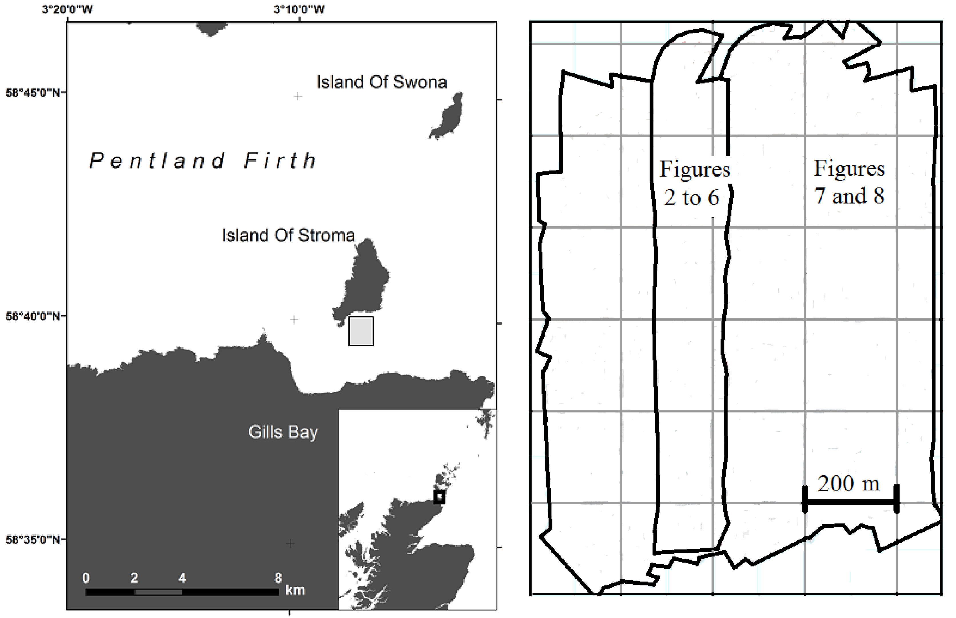
A survey was conducted on 25 June 2015 in the Inner Sound of the Pentland Firth, to the south of Stroma Island off the north coast of Caithness, Scotland, over an area of approximately 900 by 1250 m in an exploration of the seafloor in the tidally-energetic environment (
Figure 1).
The sonar was deployed from a 7 m catamaran; the “ERI Aurora”. The sonar was coupled to the vessel’s hull and suspended beneath it via a pole mounted to the side of the boat. A Hemisphere V110 GPS heading sensor was mounted directly above the sonar to measure position and vessel/sonar heading. The ping rate was approximately 7.7 Hz. The sonar trace length was 120 ms, corresponding to a maximum range and half-swath width of approximately 90 m from the sonar. The survey was conducted along 15 lines spaced at 50 m intervals running north-south approximately at right angles to the general trend of isobaths. The vessel speed relative to the seabed was approximately 4 knots (2 ms−1).
The seabed was at depths varying from approximately 40 m below the sonar vehicle across the south of the survey area shoaling to approximately 10 m at the northern end of the survey area. The bedrock is Devonian flagstone of Middle Red Sandstone age steeply dipping at approximately 50° to the east. This is exposed at the seabed over much of the survey area. It is overlain by a ridge of gravel running across the southern half of the survey area and by a sub-aqueous dune of sand underlain and surrounded by a field of cobbles in the northern half.
3. Sonar Data Processing
Geometrical spreading was compensated for in two stages. First, a time-varied gain (TVG) of +30 log(R) decibels (dB) (where R is one-way travel range in meters) was applied during data acquisition. This accounts for two-way intensity loss for point targets (inversely proportional to the fourth power of range) and for the effect of the area of the seabed ensonified by the sonar pulse (proportional to range as a far-range approximation). Secondly, the effect of the area of seabed ensonified by the sonar pulse was corrected more accurately post-acquisition, accounting for inclination angle, as well as range.
Other processes were applied post-acquisition. Corrections for absorption of +A.2R dB were applied, where A = 0.0335, 0.0600 and 0.1007 dB/m are the respective absorption coefficients for the three frequencies estimated using van Moll, Ainslie and van Vossen [
18].
The locations of the first arrival of the seabed at normal incidence on traces were determined. For a range-only sonar system, this provides the sole estimate for the depth to the seabed from the sonar, and a flat seabed across swath is assumed in subsequent processing.
The process of trace normalisation (TN) was applied. The angular response of the sonar in the vertical plane orthogonal to the sonar vehicle was normalised to the response at a reference angle in the sonar’s frame of reference (30° below the horizontal). The angular response of the seabed as a function of inclination angle estimated with respect to the seabed’s frame of reference (the grazing angle) was normalised to the seabed’s response at the reference inclination angle.
Beam functions and seabed backscatter functions are dependent on sonar carrier wave frequency. Beam functions were estimated by extraction from sonar trace and sonar vehicle roll data using the method of Tamsett and Hogarth [
6] (patent pending WO2014/170213) from just over 600 contiguous traces affected by ±5° of roll from a swath running over a rocky seabed approximately parallel to the dip direction exhibiting an approximately uniform seabed across swath. The method takes advantage of the rotation of the sonar’s frame of reference with respect to the seabed’s frame of reference during sonar vehicle roll. This enables multiple sonar beam sub-functions to be extracted with angular extent equal to the amount of roll. The multiple sub-functions are extracted in such a way that they overlap with respect to angle at their ends and may subsequently be reconciled in constructing single functions for the full range of incident angles encountered in the data. In addition to normalising data to the response at the reference inclination angle, a correction was also applied for sonar vehicle roll.
During processing of swaths, seabed backscatter functions were extracted from the nearest 201 traces centred on the trace being processed. Where swath bathymetry data are available, corrections are also applied for slope, but this cannot be done for data acquired using a range-only sonar system.
The process of slant range correction was applied to display data as a function of horizontal distance from the sonar vehicle.
Finally, the process of rendering tri-frequency acoustic amplitude for colour visualisation is applied. Humans perceive colour optically, and therefore, the acoustic frequencies are mapped to optical ones for human visualisation. This is a natural extension of the presentation of single-frequency sidescan sonar swaths as greyscale images with which we are familiar. It would seem appropriate that seabed responses at the lowest sonar frequency (114 kHz) should appear as the low-frequency optical primary colour red in the electromagnetic spectrum and that the mid-sonar frequency (256 kHz) appear as green, while the high sonar frequency (410 kHz) as blue.
The process of mapping sonar data as a function of frequency to optical primary colours can be achieved by a simple one-to-one mapping. This and other mapping methods are described in detail in a later section. The result of the simple one-to-one mapping is illustrated in
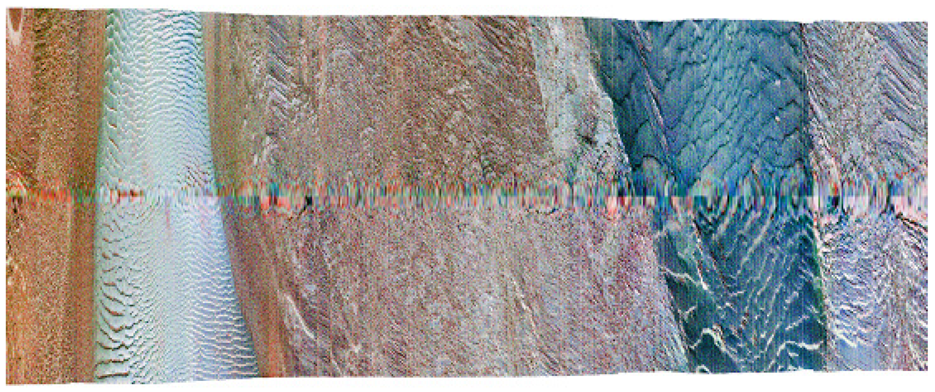
Figure 2.
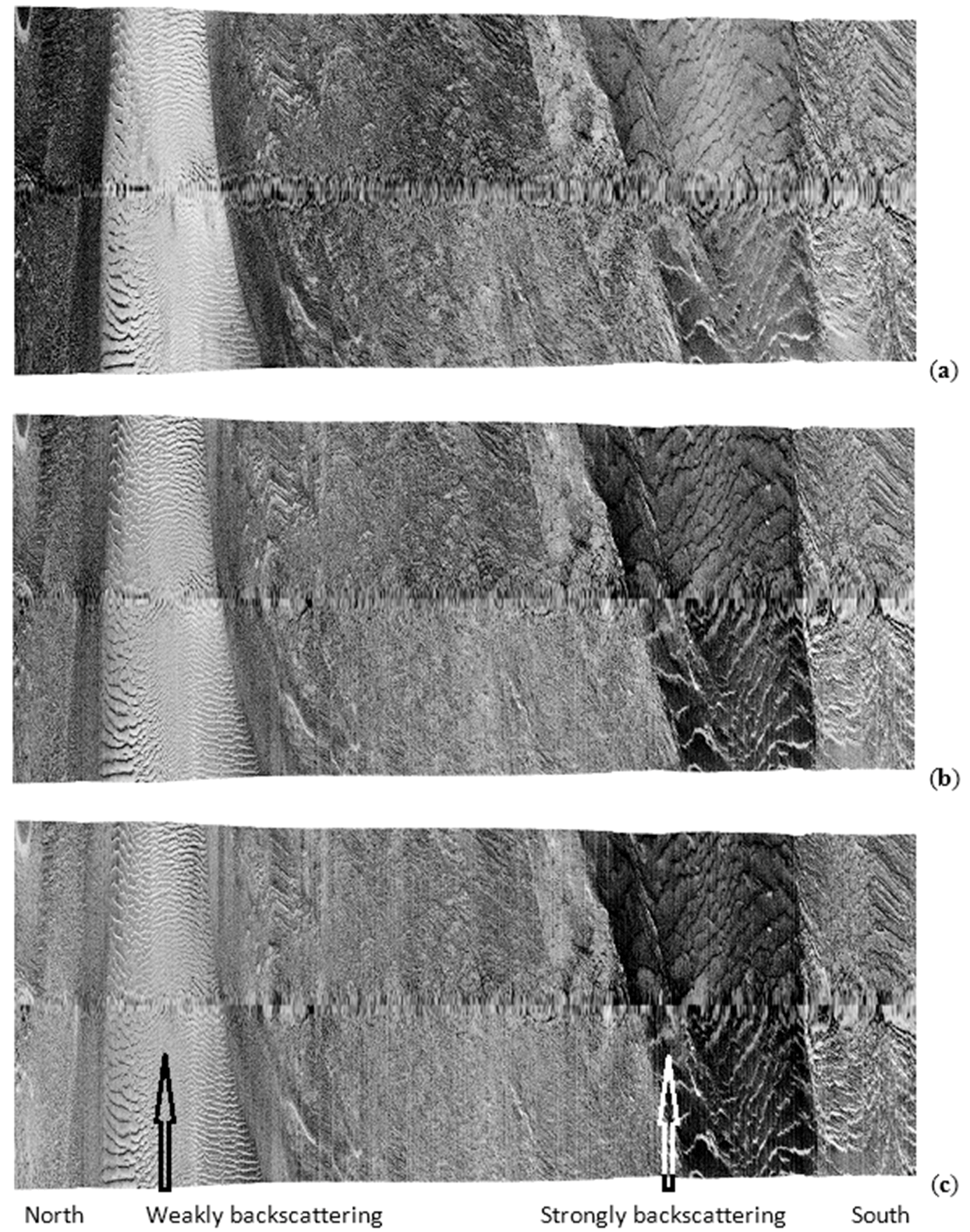
The figure also illustrates the importance of the TN process. A swath is presented as traces placed contiguously across the page from right to left, with starboard traces running up the page and port traces down the page.
Figure 2a shows a processed swath, except that the TN process has not been applied. Colour in this image has a large arbitrary component and compromises image interpretability. Indeed, it would be easier to interpret the image if it were reduced to a display of shades of grey. This illustrates the reason previously suggested for the persistence of greyscale display over the years since colour sonar was mooted in ~1970.
Figure 2b, however, shows the result of including TN. Having corrected the data for the angular shape of the beam function at each frequency by normalising the sonar response to that at the reference inclination angle (30°) and also normalising the amplitude responses of the seabed to the responses at the reference inclination angle, not only amplitude, but also colour, becomes a meaningful effect and property of the seabed. Colour now conveys additional dimensions of information on the nature of the seabed compared to greyscale imagery, thereby enhancing the interpretability of images.
4. The Acoustic Colour of the Seabed
Before considering methods for rendering multi-frequency sonar data as colour images, we look a little more deeply at the concept of the acoustic colour of the seabed.
Where a sonar system is calibrated, the calibrated backscatter amplitude response of the seabed may be computed from:
where:
Scal is the calibrated or natural amplitude response of the seabed, this being the ratio of the acoustic signal amplitude backscattered from a seabed to the signal incident on the seabed along the same line (0 to 1.0);
S is the sonar amplitude response of the seabed (a large integer) corrected for: geometrical spreading incorporating the effect of the area of the seabed ensonified by the sonar pulse, absorption, and the sonar beam function (data along the trace are normalised to the response at the reference inclination angle in the sonar’s frame of reference);
Rcal is the ratio of the amplitude response of the sonar receiver in sonar amplitude units (a large integer) to the pressure amplitude at the receiver in micro-Pascal;
Tcal is the amplitude of the sonar pulse in micro-Pascal one meter from the transmitter in the direction of the reference inclination angle.
The calibrated amplitude response of the seabed
Scal, is a function of sonar carrier wave frequency
ν and angle of incidence with respect to the frame of reference of the seabed (the grazing angle)
θ. The function
Scal(
ν,
θ) is two-dimensional and is the broadband seabed backscatter function encapsulating the acoustic backscatter characteristics of a seabed. The dependence on frequency is what makes the seabed acoustically colourful (by definition). The hyper-colour property inherent in
Scal(
ν,
θ) cannot be directly visualised. The generalised function
Scal(
ν,
θ) must be reduced to values at three discrete frequencies (or averaged over three frequency bands) and the values scaled to 8-bit values (zero to 255) for display in pixels in digital visual technologies:
The values of nDatR(θ), etc., may then be used for computing RGB components of the natural acoustic colour of the seabed for the frequencies νlow, νmed, νhigh as a function of grazing angle θ, i.e., the values may be used to present the seabed backscatter function measured by a colour sonar system as a line of colour.
To display a sonogram montage as a chart, the backscatter values along traces (across sonograms) are normalised to the seabed response at the reference inclination angle
θref, say 30° [
6]. At angles much less than normal incidence, the natural backscatter amplitudes are small and visually not very distinguishable from shadow. To generate mid-range colours more appropriate for practical human visualisation, an amplitude gain might need to be applied.
These values may be directly used as parameters for displaying colour for human visualisation or may be used as input to a process for generating other RGB parameters for colour display. Optical colour derived from these values should be specified as having been generated with respect to: the values of the carrier wave frequencies of the system (or the means of bands); the reference inclination angle; and the amplitude gain applied. The relative RGB values are objectively determined by the sonar’s calibration data.
However, for an uncalibrated system, the relative values are not known; instead, usable subjective values may be estimated by applying a process of frequency equalisation using an image as a standard for this purpose to allow colour image texture in a collection of images to be compared between images.
5. Mapping Data at Sonar Frequencies to Optical Primary Colour Frequencies
Several methods for rendering multi-frequency sonar amplitude data as optical colour for human visualisation are now described. The experimental data presented in this paper were acquired using an uncalibrated sonar system, and the methods for rendering colour are described in terms of sonar amplitude units (large integers), rather than the natural amplitudes of a calibrated system. The methods described are readily adaptable for use with natural amplitudes where data from calibrated systems are available.
5.1. RGB Colour
The simplest approach to mapping acoustic to optical colour is a one-to-one mapping of data at sonar frequencies to data at optical frequencies.
Processed sonar amplitudes are typically represented by large positive integers, which must be reduced to three 8-bit RGB values in the range of zero to 255 to display colour in pixels on digital visual display technologies.
where:
iSonarLow, iSonarMid and iSonarHigh are large integers representing the amplitude response of the seabed at three frequencies measured by the sonar system;
fScaleLow, fScaleMid and fScaleHigh are numbers (of the mathematical type, real) used to reduce the sonar amplitude responses to mid-range 8-bit numbers (zero to 255).
The values of nDatR, nDatG and nDatB are suitable for use as parameters in a computer-programed function that sets the pixel colour at a location on a digital visual display unit.
The relative values of
fScaleLow,
fScaleMid and
fScaleHigh are known if a sonar system is calibrated. For an uncalibrated system, they can be determined subjectively by a process of frequency equalisation applied to an image selected as a standard for the purpose of setting these values. First, the value for one of
fScaleLow,
fScaleMid or
fScaleHigh is explicitly set for displayed image values in the range of zero to 255 to be distributed such that the corresponding grey level image for that frequency is neither too dark nor too light (e.g., as in
Figure 3a–c). The values of the other two are than calculated such that the mean pixel colour in the image used as the standard is a shade of grey. The effect of this is that departure from grey into other colours across the standard image is optimally balanced.
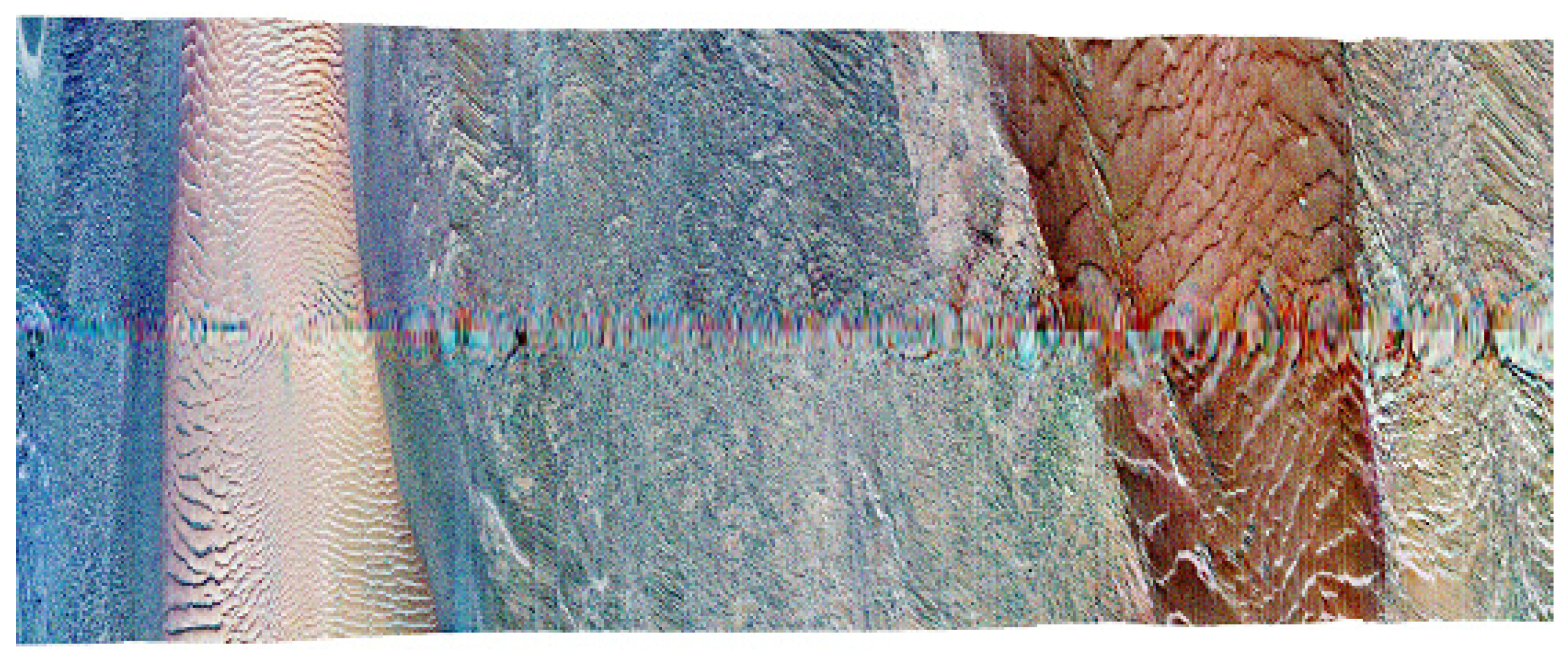
An example of a colour sonogram presented in RGB colour is shown in
Figure 2b. The values for
nDatR,
nDatG and
nDatB are proportional to the sonar amplitudes as a function of frequency. A value of zero represents shadow and appears as black. A value of 255 represents saturation and appears white. A strongly backscattering seabed appears as light shades of colour, e.g., the light shades of blue running up the right side of
Figure 2b are strongly backscattering. Conversely, a weakly backscattering seabed appears as dark shades of colour; the dark shades of blue running up the left side of
Figure 2b are a very weakly backscattering seabed.
This approach to mapping non-optical intrinsic colour data to optical colour components is the usual one, e.g., the multi-spectral multi-beam data in Hughes Clarke and Muggah [
7], the colour blending of seismic attributes in Henderson
et al. [
9] and a broadband RADARSAT image in Mayer [
16] are all displayed this way.
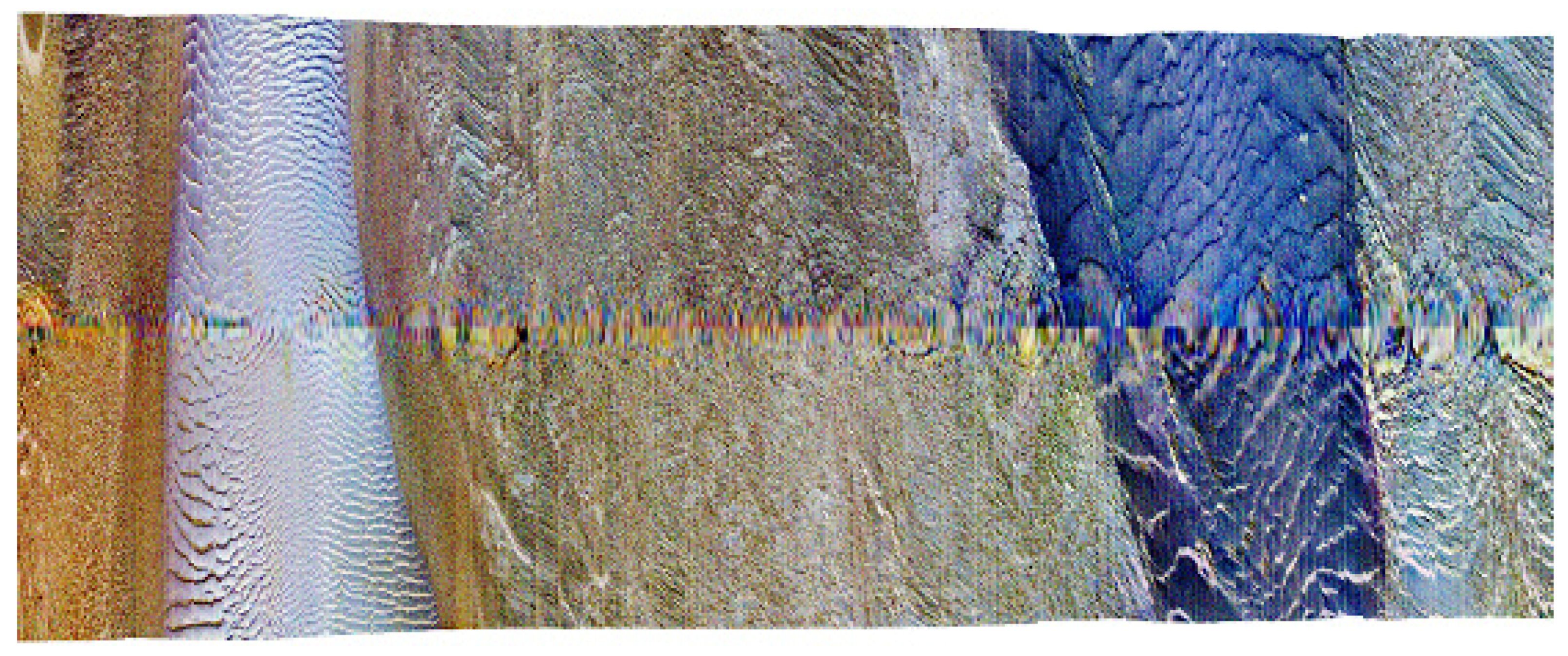
5.2. Negative RGB Colour
An alternate way to reduce sonar amplitude to image amplitude is to represent the primary colours by their negatives,
i.e.:
A value of zero now represents saturation (black), and 255 represents shadow (white). Weakly backscattering seabeds appear as light shades and strongly backscattering seabed targets as dark shades. The greyscale images in
Figure 3a,b,c are for values of
nDatR,
nDatG and
nDatB generated in this way. Negative greyscale images provide a relationship between target strength and shade of grey that most people find more conducive to interpretation than positive greyscale images do, and this is how greyscale images are more commonly displayed. However, when these are added to generate a colour image (
Figure 4), seabeds that more strongly backscatter the high-frequency than the low-frequency signal appear as shades of red instead of blue, and seabeds that more strongly backscatter the low-frequency than the high-frequency signal appear as shades of blue instead of red. This is an undesired outcome.
5.3. Negative BGR Colour
For shades of red, green and blue to be seen in proportion to the relative backscatter amplitudes of the low-, mid- and high-frequency sonar data, respectively, the negative RBG colour scheme can be adapted by switching
nDatR and
nDatB in the computation of the values of
nDatR,
nDatG and
nDatB. We refer to this colour scheme as negative BGR colour:
The result is shown in
Figure 5. Shadow is represented by white; saturation by black; the darkness of a colour is proportional to seabed backscattering amplitude; and shades of red, green and blue are seen in proportion to the relative backscattering amplitudes of the low-, mid- and high-frequency sonar data, respectively.
5.4. Negative CMY Colour (Negative Complementary RGB Colour)
An alternative way to achieve a colour image with properties similar to those for negative BGR colour is to construct the primitive colour components in this way:
The negative 8-bit representation of the low-frequency sonar data feeds into both green and blue. The colours green and blue additively mix to produce cyan. Similarly, the mid-frequency data feed into red and blue, which mix to produce magenta, and the high-frequency data feed into red and green, which mix to produce yellow. We refer to this colour mapping scheme as negative CMY colour. The colours cyan, magenta and yellow (CMY) are the additive complements of red, green and blue, respectively. The colour scheme therefore could alternatively be referred to as negative complementary RGB colour.
The effect of averaging sonar amplitudes when pairs of data are merged is to suppress the contrast in colour in the result,
i.e., the departures from the mean of
nDatR,
nDatG and
nDatB are less than the departures from the mean of the three 8-bit sonar data used to compute them. This however can readily be compensated for by applying a colour contrast gain as a second stage to computing negative CMY colour. At every pixel, the departure of the values for the primary colour data from their mean is multiplied by the
ColourGain factor:
and similarly for
nDatG and
nDatB. Any resulting values that outlie the range of zero to 255 are set to the limiting value.
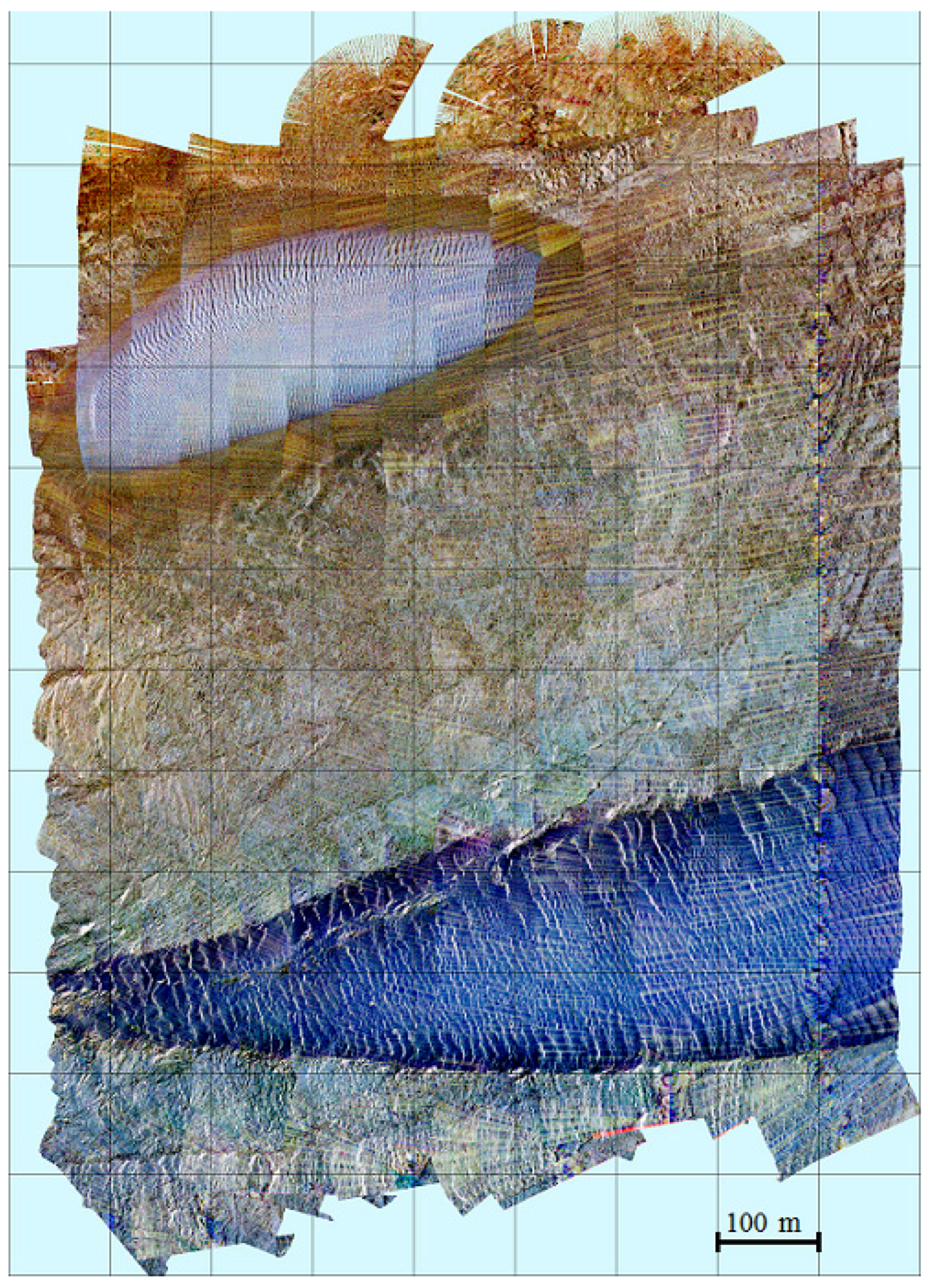
A
ColourGain of two is an appropriate value to apply as a default value. An example of a colour sonogram shown in negative CMY colour is shown in
Figure 6.
Where colour contrasts are subtle and difficult to see, colour gain by a factor greater than two (e.g., three or four) may be applied to amplify subtle colour contrasts to make them more visible (this applies to all of the colour schemes, not just to negative CMY colour).
The result for negative CMY colour (
Figure 6) is similar in its characteristics to those for negative BGR colour (
Figure 5).
5.5. Discussion
Of the colour schemes outlined, in our opinion, the ones that generate colours most harmonious with human visualisation and best enhance images for interpretation are negative BGR and negative CMY colour. However this is a matter of subjective opinion, rather than objective correctness, and other people might form a different opinion.
The negative BGR and negative CMY colour schemes yield shades and hues in response to seabed backscattering strengths in which shadow is represented by white; saturation by black; the darkness of a colour is proportional to seabed backscattering amplitude; and shades of red, green and blue are seen in proportion to the relative backscattering amplitudes of the low-, mid- and high-frequency sonar data, respectively.
To attempt to provide some rationale for the preference expressed for negative BGR and negative CMY, as creatures of the day rather than the night, we are more used to seeing objects against a light background (e.g., this ink is black and the page is white) rather than vice versa. Thus, whilst representing shadow by white and saturation by black sounds contradictory, it is certainly the more common (though not universal) way to represent greyscale sonar and sub-seabed acoustic images.
The colours generated by simple RGB colour tend to have an iridescent quality, most likely a side-effect of brightness increasing with signal strength, which we find strident.
The colours generated by the negative CMY colour scheme in contrast have a particularly pastel quality, which is pleasing to and gentle on the eye. The mathematical symmetry of the parameters in the computation for this scheme conveys the suggestion of something intrinsically attractive.
The colours generated by negative BGR colour are bolder and more simply computed than those for negative CMY colour.
We recommend the negative BGR colour and negative CMY colour schemes and propose that after more experience is gained in their use, that one of these be considered for adoption as a standard for the presentation of multi-frequency sonar data as colour images.
6. Swath Montage Charts
It is seen in the processed images for the single swath featured in
Figure 2,
Figure 3,
Figure 4,
Figure 5 and
Figure 6, that the central suture line of the swath corresponding to normal incidence at the seabed, where the port and starboard halves of the image join, has a compromised scar-like appearance. This is typically difficult to completely eliminate, particularly for data acquired using a range-only sidescan sonar. However, swaths with a 90 m range to port and starboard acquired along lines spaced 50 m apart may be overlain in generating a chart, and any scar associated with normal incidence may be visible along the length of only the last swath added to the chart.
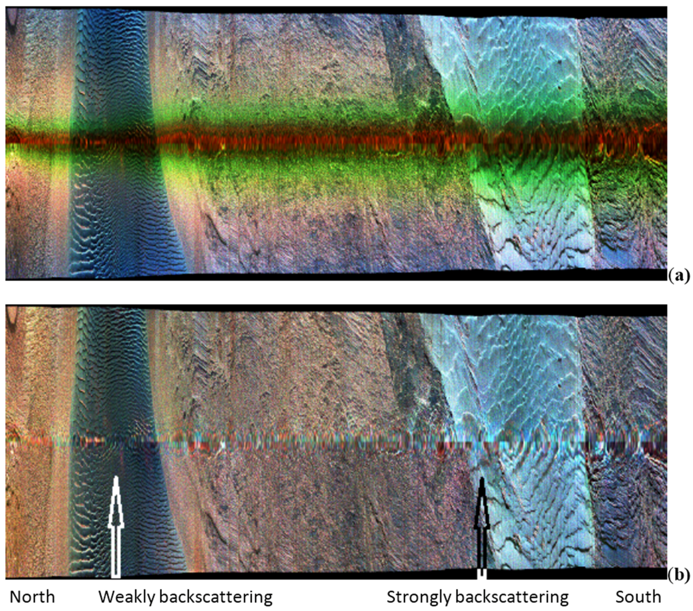
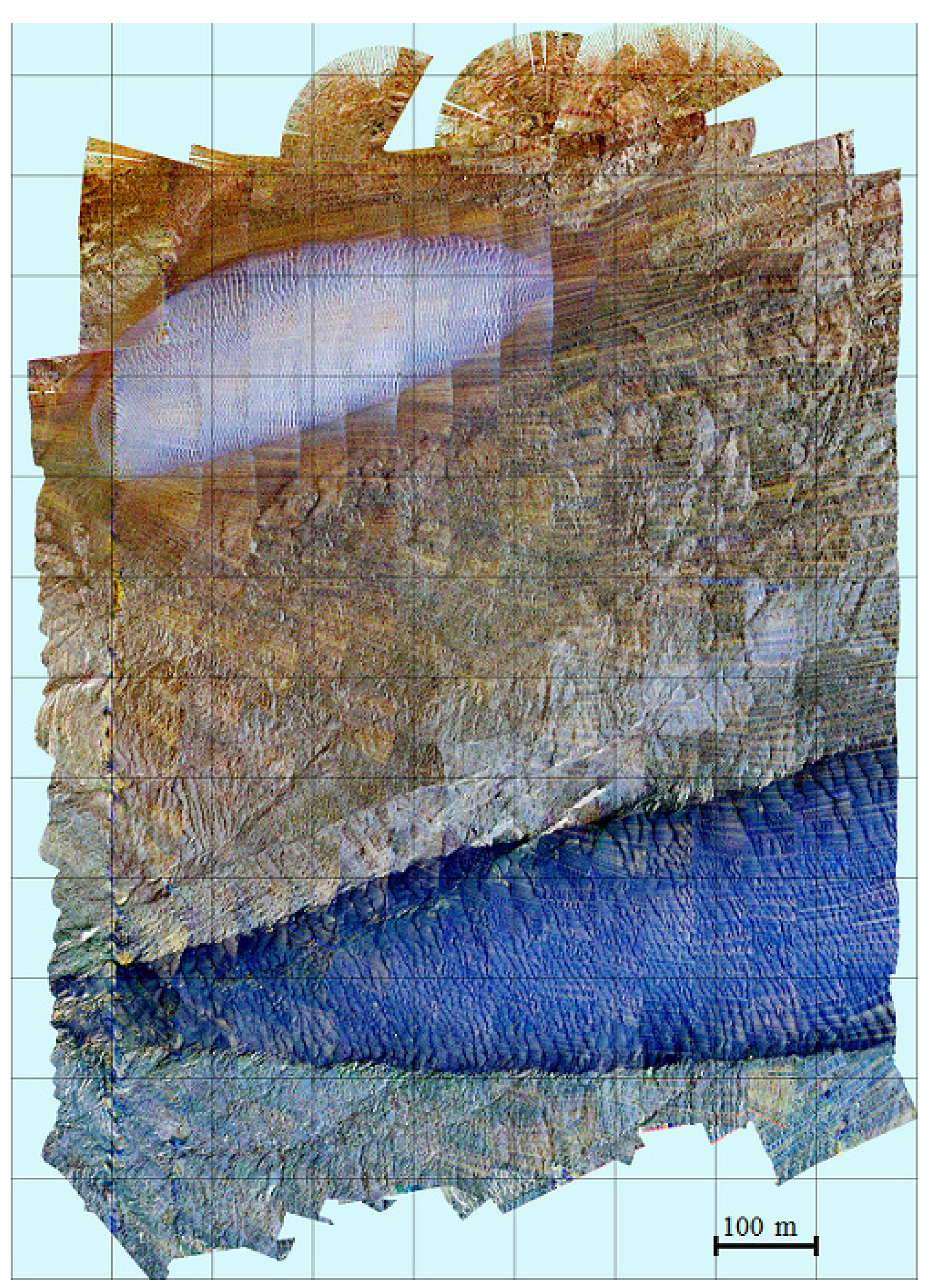
A montage of swath sonograms is shown as a chart in
Figure 7. The swaths are overlain from left to right, and the direction of ensonification is therefore to the left, or to the west; except for the easternmost half-swath down the right-hand side.
Figure 8 shows the chart for swaths overlain from right to left, and the direction of ensonification is to the east/right; except for the westernmost half-swath down the left-hand side. The colour for both figures was generated using the negative BGR colour scheme.
Frequency equalisation was applied to the image in
Figure 7 to achieve an appropriate colour balance over the whole image. This image being equalised with respect to itself means that the relative amplitudes in the RGB components of the colours generated are subjective and lack the degree of objectivity that would be present in colours generated using a calibrated system.
Nevertheless, all colour sonar images equalised using the frequency equalisation parameters extracted from the image in
Figure 7 may be compared to each other and the colour within the collection of images regarded as a property or characteristic of the seabed.
The sidescan sonar data were acquired as part of a multi-disciplinary and integrated investigation of the high energy tidal environment of the Inner Sound of the Pentland Firth (McIlvenny
et al. [
19]), where tidal currents are up to ~6 ms
−1. The sonar data provide information on the seabed characteristics and sedimentary dynamics to inform a potential exploitation of a renewable energy resource. The sonar data have a more restricted use in this paper, which is to illustrate the description of the colour sonar technique and provide a demonstration of its utility. Only brief descriptions and interpretations of some principal seabed features seen in the images are given here.
A wedge-shaped rippled bank of material appearing in shades of royal blue runs across the lower half of the image. This is known from grab samples distributed along the centre of the ridge to be composed of fine gravel-sized broken shell. The changes in colour from very dark blue along the edges of the bank to lighter shades of blue along the centre indicate changes in the size of gravel-sized particles from the edges to the centre. The tidal current at the time of data acquisition was to the west, and the faces of westward facing scarps in the ripples cast shadows (white) in
Figure 7 and are ensonified and strongly backscattered (black) in
Figure 8. The ripples along the edges of the bank have greater amplitude and are more widely spaced than those along the centre of the bank. The direction of the ripple scarps reverses when the direction of the current during the tidal cycle is to the east [
19].
It is instructive to consider the individual responses of the gravel ridge to sonar signal as a function of frequency by inspecting the single-frequency swaths collected in
Figure 3. The gravel ridge runs down the right-hand half of the figure. It can be seen that the response to the low-frequency signal (
Figure 3a) is relatively weak and that the high-frequency response is strong. Gradation in the strength of the response of the seabed across the gravel ridge at all frequencies can also be seen.
There is an oval-shaped subaqueous dune of material appearing in shades of very light blues and purples at the top of
Figure 7 and
Figure 8. This is surrounded by a halo of material appearing as shades of hazel brown. The light blue/purple material is medium sand. The hazel brown material is a bank of small cobble-sized stones 4 to 6 cm across accommodating thinly-distributed growths of kelp seaweed. The sand is rippled with scarps facing west across the top of the dune and east across the bottom (throughout the tidal cycle). The dune is associated with a gyre or eddy, which is driven anti-clockwise during flood tide (currents to the east in the main channel), but which sits in a tidal current shadow during the ebb tide [
19]. The ripples across the top of the dune can be seen to be isolated sub-dunes sufficiently separated in places to see the hazel brown-coloured cobble bank that underlies the sand dune.
It is seen again here that there are indications in the colour sonar data of a change in the grade of sand across the sand dune. The sand at the centre is more weakly backscattering (lighter shades) than it is at the edges, indicating that the sand at the centre where the currents are at their weakest is a finer grade than at the edges.
Consider again the response of the sand dune and its immediate environs as a function of frequency (
Figure 3). The dune runs down the left-hand half of the figure. The response of the sand at all frequencies is weak. A cursory glance might suggest lines of strong response at the low frequency, but this is in fact the strong response at that frequency of the cobbles that form the halo surrounding the dune where the cobbles are present as linear features between isolated sub-dunes across the northern half of the large-scale dune.
Of particular interest is evidence of colour anisotropy (the dependency of colour on the direction of ensonification) in the halo around the dune, particularly south of the dune. In the image in which ensonification is to the west (
Figure 7), the colour is a bolder shade of brown and has a more strongly demarcated boundary with the seabed further to the south compared to the image in which ensonification is to the east (
Figure 8). We will not speculate here on possible causes or explanations of the colour anisotropy observed at this location.
The seabed across the rest of the survey area is essentially exposed rock. Rock often appears as complex image texture in sidescan sonar records. Structures at the interfaces between dipping strata and along fault lines are associated with a plethora of interlocking linear features. What is surprising is the variety of colour in the sonic response of the exposed rock across the seabed, varying from a complex collection of shades of red, brown and green in the northern half of the survey area to a similarly complex collection of shades of blue and grey in the southern half of the survey area. Video footage of the seabed obtained from underwater vehicles suggests this is likely to be largely due to a relative absence of thinly-distributed sedimentary material on the seabed across the southern half of the survey area compared to the northern half [
19]. However, of interest is the anisotropic response of the rocky seabed between the oval dune and gravel ridge. This is rather light grey to ensonification to the west (
Figure 7) and darker shades of brown to ensonification to the east (
Figure 8). This might be a result of fine asymmetrically-disposed structures associated with strata dipping to the east. There is also a band of seabed immediately north of the centre of the gravel ridge that is shades of green and light blue to ensonification to the west (
Figure 7), but shades of light violet to ensonification to the east (
Figure 8).
There are non-seabed effects or artefacts in the images. Patches of light-coloured streaking can be seen in places, in particular at the eastern end of the cobble halo around the oval sand dune resulting from aeration in the water column due to vessel wake from previous lines and the preferential attenuation of the low-frequency signal. Secondly, there is a linear texture across many swaths due to imperfect measurement of roll by the sonar’s attitude sensor and correspondingly imperfect corrections for the effects of roll. This situation would be expected to considerably improve through the use of a higher specification measurement reference unit for measuring attitude.
7. Natural Sonar
Human vision perceives as colour the optical part of the electromagnetic spectrum spanning less than an octave of the spectrum. The three frequencies in the sidescan sonar system described in this article represent a frequency range of almost two octaves. The information on colour inherent in anthropic multi-frequency sonar data is not directly perceived acoustically, but indirectly by mapping data at sonic frequencies to optical ones for human colour visualisation. However, we might ask whether the mental world view (the image of reality) of animals informed by natural sonar incorporates colour perception?
That certain animals have the capacity to construct mental world views from “echo location” was recognised by the late 1950s (Griffin [
20]) in the wake of early developments in anthropic sonar technology (e.g., Chesterman, Clynick and Stride [
21]), and it seems likely that the development of anthropic sonar inspired hypotheses about natural sonar. Two kinds of animal are well known for ultrasound sonar capability: toothed whales (dolphins, porpoises, river dolphins, killer whales, sperm whales); and Microchiropteran bats (Au and Simmons [
22]). Certain species of shrew also possess ultrasound sonar (Siemers
et al. [
23]).
The bottlenose dolphin is typical of toothed whales. It generates short (~70 microsecond) 120 to 130 kHz pulses (Au [
24]). The “ping” is remarkable for being similar to those generated in anthropic single-frequency sonar systems. The narrowness of the frequency range has the attribute of facilitating strong directionality that dolphins appear to exploit for acoustic probing along a line. Being an essentially single-frequency system, dolphins’ sonar does not satisfy the information criteria for colour perception.
Sonar in bats, however, is a different matter. For example, the pulse generated by the “common little brown bat” is a long downward sweeping frequency-modulated one, beginning with a frequency of 100 kHz and ending at 40 kHz over two milliseconds (Davies [
25]). Similarly, the pulse generated by the “big brown bat” begins with a frequency of 100 kHz and ends at ~20 kHz, with a flat spectrum over the range 25 kHz to 90 kHz (central frequency 60 kHz), and incorporates multiple harmonics, over five milliseconds (Simmons
et al. [
26]; Galambos and Simmons [
27]).
A frequency swept “chirp” pulse is an alternative to multiple discrete frequency pings to achieve multi-frequency sonar. The bandwidth in bats’ sonar is approximately two octaves. Whilst a broad bandwidth allows accurate estimates of distance to target ([
26]; Barber
et al. [
28]), another use might be acoustic colour perception (Dawkins [
29]). Neural-ware employed in the evolutionary past for interpreting visual colour stimuli might be redeployed for interpreting aural colour stimuli [
29]. Significantly, a small proportion of humans experience synaesthesia and visualise colour in response to aural stimuli, implying a connection for a multi-frequency aural signal originating in the ear to parts of the brain normally dedicated to processing a visual signal originating in the eye. This is evidence for a disposition for neural-ware usually associated with one sense system to interact with another. Over time, under evolutionary pressure, a change in the principal allegiance might occur.
For sonic colour perception in nature to be real, it must convey an evolutionary advantage (Simmons and Stein [
30]). Colour sonar would be expected to convey similar advantages as colour vision. Finding food and avoiding becoming food are the most fundamental requirements, and it is likely that colour would facilitate these. There is vegetation adapted for pollination by bats bearing flowers that are conspicuous under ultrasound radiation (Simon
et al. [
31]). By analogy to conventional flowers, which are universally colourful to birds and insects, so might flowers adapted to backscattering ultrasound be similarly brightly colourful to bats. It is likely that there would be a role in sexual selection. It is intriguing to imagine how bats might appear to each other. Bats are monotonously uncolourful to visible e-m radiation. If bats are significantly more colourful to ultrasonic radiation, this would constitute evidence for ultrasound colour perception in bats. This could be investigated through the acquisition of multiple frequency ultrasound images of bats.
Anthropic dual-frequency sonar systems commonly employ frequencies of approximately 100 kHz and 500 kHz for investigations to distances of the order of tens of meters. The ~2 octave bandwidth is similar to the range used by bats, though the frequencies in the anthropic systems are about a factor of five greater; but in water, the transmission velocity is greater by the same factor, so in fact, the range in wavelengths is very similar. This would appear to be a remarkable coincidence.
8. Summary Remarks
Multi-frequency sidescan sonar trace amplitudes were corrected for non-seabed effects and the effect of seabed backscatter functions were normalised to the seabed response at a reference grazing angle (30°). Reducing sonar amplitude to an effect of the seabed normalised to the seabed response at the reference grazing angle has the side effect that acoustic colour generated from multi-frequency data becomes a meaningful property or characteristic of the seabed (with respect to the reference grazing angle). The additional information inherent in colour over greyscale data enhances the interpretability of data, allowing greater discrimination between different seabed image textures.
A prototype three-frequency sidescan sonar system (114, 256, 410 kHz) deployed in the Inner Sound of the Pentland Firth, Scotland, has provided data for an area of the seabed of approximately 900 m by 1250 m from 15 swaths. These experimental data are used to illustrate methods for rendering acoustic colour as optical colour images for human visualisation. The negative BGR and negative CMY methods generate colours with these characteristics: shadow appears as white and saturation as black; weakly backscattering seabeds appear as light shades of colour and strongly backscattering seabeds as dark shades; shades of red, green and blue are formed in proportion to the relative backscattering amplitudes of the low-, mid- and high-frequency sonar data, respectively. In our opinion, these characteristics facilitate interpretation; however, we acknowledge this is a subjective judgement that other workers might not share.
The experimental data acquired in the Pentland Firth reveal a seabed having a wide variety of colourful acoustic image textures. Bedrock exposed at the seabed is associated with complex textures in shades of a wide variety of colours. A fine gravel bar of broken shell running across the southern half of the survey area is strongly backscattering at the higher frequencies and appears as a variety of dark shades of royal blue (negative BGR colour). An oval-shaped dune of sand in the northern half of the survey area is weakly backscattering at all frequencies and shows as a variety of shades of very light blue and purple. A halo of small cobbles around the sand dune is strongly backscattering at the lower frequencies and appears as dark shades of hazel brown. Of particular interest is evidence for colour anisotropy, i.e., a dependence of colour on the direction of ensonification. A program of seabed sampling and AUV video capture is required to investigate the causes to understand the phenomenon.
Seabed acoustic colour data could also be acquired using montaged charts from multiple single-frequency surveys for different carrier wave frequencies or by adapting broadband chirp systems to incorporate multiple bandpass filtration. A difficulty with the latter approach is that in current ultrasound sonar technologies, the range in frequency in the chirp pulses is small, falling far short of two octaves, and the seabed may not be sufficiently colourful over such restricted ranges. This restriction, however, does not apply to lower frequency broadband sub-seabed profiler technologies (e.g., 1 to 11 kHz).
Emerging from a synthesis of anthropic sonar with natural sonar is the intriguing hypothesis that Microchiropteran bats (perhaps amongst other animals, such as certain species of shrew) perceive colour in their mental world views informed by natural sonar.


