Article

Geometry of Wave-Formed Orbital Ripples in Coarse Sand

by
Gerben Ruessink
*,
Joost A. Brinkkemper
and
Maarten G. Kleinhans
Department of Physical Geography, Faculty of Geosciences, Utrecht University, P.O. Box 80.115, 3508 TC Utrecht, The Netherlands
*
Author to whom correspondence should be addressed.
J. Mar. Sci. Eng. 2015, 3(4), 1568-1594; https://doi.org/10.3390/jmse3041568
Submission received: 3 November 2015 / Revised: 3 December 2015 / Accepted: 14 December 2015 / Published: 21 December 2015
(This article belongs to the Special Issue Coastal Morphodynamics)

Abstract

:
Using new large-scale wave-flume experiments we examine the cross-section and planform geometry of wave-formed ripples in coarse sand (median grain size D 50 = 430 μm) under high-energy shoaling and plunging random waves. We find that the ripples remain orbital for the full range of encountered conditions, even for wave forcing when in finer sand the ripple length λ r is known to become independent of the near-bed orbital diameter d s (anorbital ripples). The proportionality between λ r and d s is not constant, but decreases from about 0.55 for d s / D 50 1400 to about 0.27 for d s / D 50 11 , 500 . Analogously, ripple height η r increases with d s , but the constant of proportionally decreases from about 0.08 for d s / D 50 1400 to about 0.02 for d s / D 50 > 8000 . In contrast to earlier observations of coarse-grained two-dimensional wave ripples under mild wave conditions, the ripple planform changes with the wave Reynolds number from quasi two-dimensional vortex ripples, through oval mounds with ripples attached from different directions, to strongly subdued hummocky-type features. Finally, we combine our data with existing mild-wave coarse-grain ripple data to develop new equilibrium predictors for ripple length, height and steepness suitable for a wide range of wave conditions and a D 50 larger than about 300 μm.

1. Introduction

Wave-formed ripples are ubiquitous small-scale bed forms in shelf to nearshore water depths with typical spacing (or, wave length) of O (0.1–1) m and height of O (0.01–0.1) m. Hydrodynamic and morphodynamic models often demand predictions of cross-section (i.e., ripple spacing or wavelength, and height) and planform (orientation and along-crest regularity) ripple geometry, e.g., [1,2,3], because of the effect of ripples on waves, currents, and sediment suspension and transport. Accordingly, numerous empirical classification schemes and predictors have been proposed that relate ripple occurrence and equilibrium geometry to non-dimensional wave and sediment properties; for a recent overview, see [4]. While such schemes and predictors are now reaching considerable skill for sand with typical median diameters of 150–250 μm [4,5,6], there is considerable doubt on their applicability to ripples that form in coarser sand, especially for high-energy wave conditions [6,7,8].
One of the most commonly adopted wave-ripple classification schemes for 150–250 μm sand, due to Clifton [9], comprises orbital, suborbital and anorbital ripples and expresses wave forcing and sand characteristics as the ratio between orbital diameter and median grain size, d / D 50 . For mild wave conditions ( d / D 50 2000 ) ripple length λ and height η scale linearly with d, with often-quoted constants of proportionality of about 0.65 and 0.10, e.g., [10,11], respectively. The steepness ϑ = η / λ of orbital ripples is thus near 0.15, implying them to be sufficiently steep to shed sand-laden vortices into the water column during flow reversal (vortex ripples; e.g., [12]). For energetic wave conditions ( d / D 50 5000 ; [11,13]) the ripples are anorbital; that is, λ does not depend on d anymore. Instead, λ now relates to D 50 as 535 D 50 on average, e.g., [11,14], implying that anorbital λ is substantially shorter than d. In addition, anorbital ripples are no longer vortex ripples; with an increase in d / D 50 their steepness reduces rapidly to 0.01 [11], which is essentially flat bed. Suborbital ripples from a transitional type between orbital and anorbital ripples. Predictors that are, at least partly, based on the orbital-suborbital-anorbital scheme include Wiberg and Harris [11], Soulsby et al. [15] and Nelson et al. [4]. Often, anorbital ripples are superimposed on substantially longer, three-dimensional and also strongly subdued ripples, known as large wave ripples, mega-ripples or hummocks, e.g., [16,17,18,19,20], which these predictors do not consider. The combination of anorbital ripples and hummocks has been found in the field for sand with a D 50 up to about 300 μm, e.g., [17,19,20].
Observations of wave ripples in coarser sediment are largely limited to mild wave conditions because of large water depths or low wave heights, e.g., [7,21,22,23,24,25,26]. They mostly show two-dimensional, steep (vortex) orbital or suborbital ripples with similar λ / d ratios as observed in finer sand. Limited laboratory experiments under stronger wave conditions ( d / D 50 5000–7500; [8,27]) do not show a transition to anorbital length scales or to large hummocky ripples. Instead, the ripples remain two-dimensional vortex ripples. Cummings et al. [8] found the ratio for λ / d to be lower (0.4) in 0.8-mm sand than in 0.12-mm sand (0.6) for the same d, while the experiments of Pedocchi and Garcia [27] suggest a negative dependence on the maximum orbital velocity. Whether the steep coarse-grained ripples remain orbital and develop into hummocks under even stronger wave forcing is not known. Interestingly, O’Donoghue et al. [28] postulated that ripples remain two-dimensional when D 50 exceeds 300 μm and are three-dimensional for D 50 is less than 220 μm, except when d is low. Other data [5,29] suggest that even coarse-grain ripples may become three-dimensional under strong wave forcing. This paper documents new coarse-sand, equilibrium ripple data collected for the d / D 50 1000–20,000 range under high-energy shoaling and plunging random waves on a prototype laboratory beach. Our objectives are to investigate cross-section and planform ripple geometry and to derive a new coarse-sand equilibrium ripple predictor for which we combine our data with several existing coarse-grain ripple data sets collected under mild wave conditions.

2. Methods

2.1. Bardex II Experiment

The data analysed here were collected in the large-scale Delta flume facility of Deltares in Vollenhove, The Netherlands as part of the second Barrier Dynamics Experiment (Bardex II; [30]). The barrier, which filled the entire 5-m width of the flume, was constructed from coarse ( D 50 = 430 μm; mean grain size = 510 μm; D 16 = 280 μm; D 84 = 830 μm), moderately sorted ( 0 . 81 ϕ ) and coarse-skewed ( 0 . 24 ϕ ) quartz sand that contained a small amount of gravel (≈1%, >2000 μm) [30]. The median fall velocity w s of this sand amounts to 0.061 m/s [31] and the Reynolds particle number R e p = g R D 50 D 50 / ν [5] to 35.9, where g = 9 . 81 m/s 2 is gravitational acceleration, R = 1 . 65 is the submerged specific density, and ν is the kinematic viscosity of water, here set to 1 × 10 6 m 2 /s. The seaward part of the barrier profile initially comprised a 0.5-m thick sand layer at cross-shore coordinates x = 29–49 m ( x = 0 is at the wave paddle) and a 1:15 seaward-sloping section at x = 49–109 m (Figure 1) that ended at the 4.5-m high barrier crest.
Figure 1. Initial bed elevation z versus cross-shore distance x from the wave paddle (brown line). The blue line is the default still water level h s ; the two dashed blue lines represent the lower and upper h s , see Table 1. The 16 triangles represent the locations of pressure transducers. At the 4 open triangles the pressure transducer was co-located with an electromagnetic or acoustic current meter. The filled circle is the approximate location of the 3D Profiling Sonar.
Jmse 03 01568 g001
The Bardex II test programme consisted of 19 distinct tests with different wave and water level conditions, grouped into 5 series that focused on surf-swash zone processes (series A–C), and barrier overwash and destruction (series D and E, respectively). The wave paddle steering signal in all tests was constructed from a JONSWAP spectrum using a target significant wave height H s 0 and peak wave period T p 0 with a peak-enhancement factor of 3.3. As can be seen in Table 1, H s 0 was either 0.6 or 0.8 m, and T p 0 varied from 4 to 12 s. The still water level h s with respect to the concrete flume floor ranged between 2.25 and 4.2 m, with a default value of 3 m (Table 1). During series C, the barrier was subjected to a rising (C1) and falling tide (C2). The Automated Reflection Compensator was switched on during all tests to avoid seiching in the flume.
Table 1. Experimental conditions during Bardex II. H s = significant wave height; T p = peak wave period; h s = still water level with respect to the concrete flume floor; T test = test duration; and N runs is number of wave runs.
Test H s 0 (m) T p 0 (s) H s 1 (m) T p 1 (s) h s (m) T test (min) N runs
A10.880.928.0332013
A20.880.908.032005
A30.880.907.931971
A40.880.908.032005
A60.6120.7311.8333513
A70.6120.7712.632135
A80.6120.7912.632005
B10.880.918.331655
B20.880.917.82.52556
C10.8, 0.680.90, 0.577.32.25 → 3.6533011
C20.8, 0.680.91, 0.587.53.53 → 2.252709
D10.840.794.03.15 → 4.21608
D20.850.824.63.45 → 4.051005
D30.860.866.03.45 → 3.9804
D40.870.847.03.45 → 3.9804
D50.880.867.73.45 → 3.75603
D60.890.879.33.30 → 3.75804
D70.8100.9310.03.15 → 3.6804
E10.880.947.43.9655
The H s 0 and T p 0 were target values at the wave paddle. The measured values at the most offshore pressure transducer ( H s 1 and T p 1 at x = 36 . 2 m, Figure 1) differed from these target values and varied slightly between runs, see, for example, Figure 5d,j. The H s 1 and T p 1 listed here are values averaged over the runs. The final 17 min of A3 are labeled as A5 in Masselink et al. [30] and involved 8 short (2-min each) sequences of mono- and bi-chromatic wave runs.

2.2. Measurements: Ripple Data
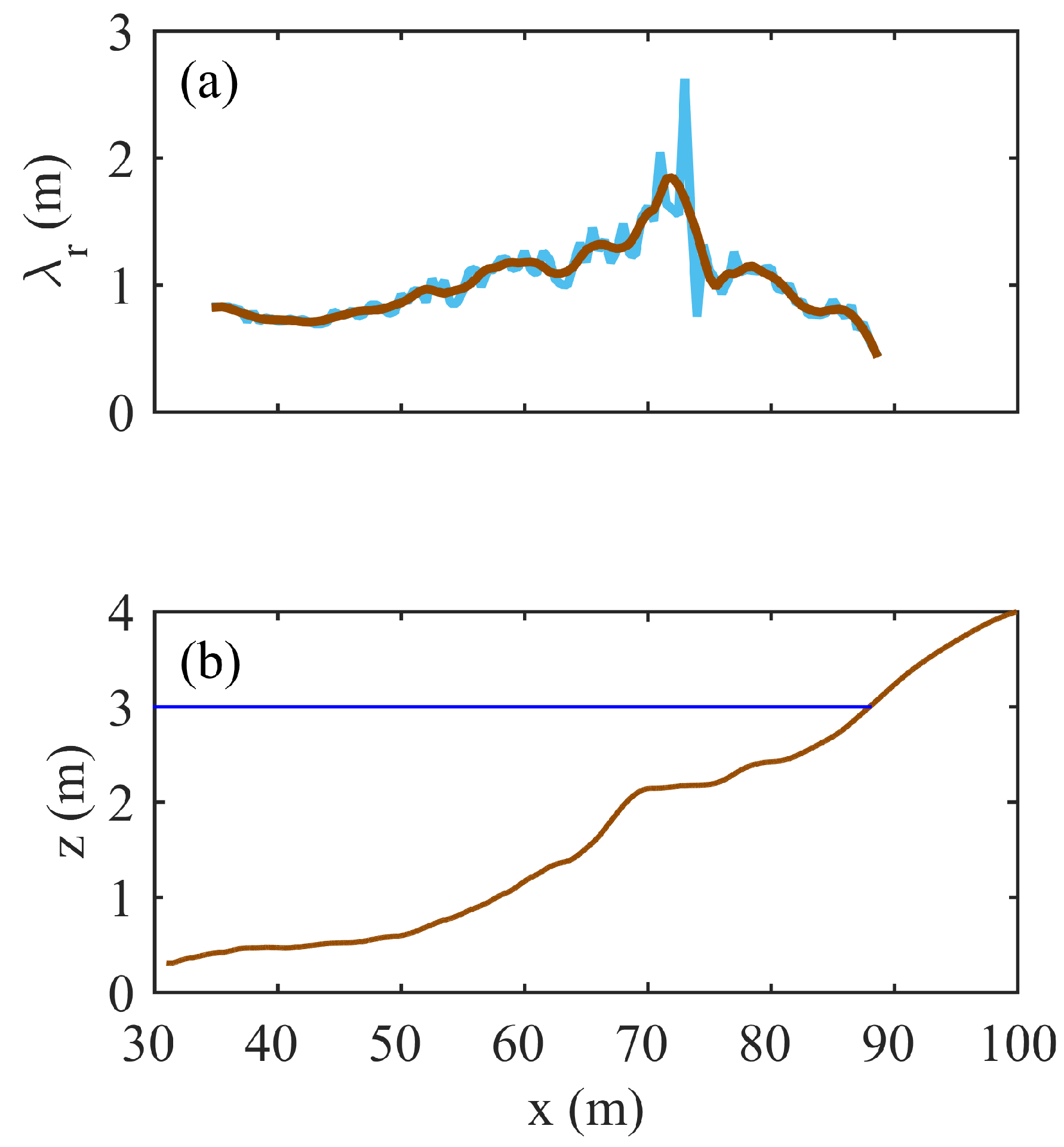
2.2.1. Profile Data

Each test was generally broken up in several wave runs (Table 1) that varied in duration from 10 min to 3 h. The center profile of the flume was surveyed after each wave run using a profiling wheel mounted on an overhead gantry. In total, 115 bed profiles were collected, each with a 0.01-m cross-shore resolution. A first inspection of the data revealed the presence of occasional spikes in most bed profiles, most likely induced by glitches in the profiling system. These spikes were removed by filtering each bed profile using a second-order loess interpolator [32] with a cross-shore scale parameter l x of 0.05 m. This interpolator acts as a low-pass filter and removes variability with length scales less than l x / 0 . 7 (here, ≈0.07 m). Visual inspection of original and despiked bed profiles illustrated that this l x was effective in removing the spikes while leaving the ripples unaffected. The despiked data are henceforth referred to as z ( x , t ) , where z is bed elevation defined positive upward from the concrete floor of the flume and t is time with t = 0 corresponding to the start of the first wave run in test A1.
Analysis of z ( x , t ) [33] revealed that the waves in tests A1–A4 ( H s = 0 . 8 m, T p = 8 s) reshaped the initially planar profile into a sandbar-trough system, with the sandbar crest at x 70 m. The waves in subsequent A6–A8 tests ( H s = 0 . 6 m, T p = 12 s) transported sand onshore, causing the decay of the sandbar and the generation of a pronounced berm in the upper swash zone. During series B and C the berm and the remains of the sandbar hardly changed, while during series D and E morphological change was most pronounced at the berm and the barrier crest [34].
To separate the large-scale sandbar-berm variability from the smaller scale wave ripples, z ( x , t ) was low-pass filtered with l x = 3 . 5 m yielding z b b ( x , t ) , the data set that contains the sandbar-berm variability only. The residual series from this filtering step, i.e., z b b ( x , t ) z ( x , t ) , are zero-mean profiles with bed variability induced by wave ripples, z ˜ w r ( x , t ) . Positive and negative z ˜ w r correspond to ripple crests and troughs, respectively. The cross-shore evolution in ripple length λ r , ripple height η r , and ripple steepness ϑ r = η r / λ r were subsequently calculated every 0.5 m from overlapping (95%) 10-m wide, centered windows (subsets) of z w r ( x ) . In each window the length and height of every individual ripple, defined with a zero-down-crossing technique, were determined. The window ripple length was taken as the mean of the individual lengths, and the window ripple height as the root-mean-square value of the individual heights. The center of the most seaward window was taken at x = 35 m, while the center of the most landward window was chosen at the location where the corresponding z b b profile intersected the still water level h s . This implies that this most landward window essentially encapsulated the swash zone. The use of 10-m windows was a compromise between having sufficient ripples within a window for robust statistics and quantifying cross-shore trends in λ r and η r . A first inspection of the length and height profiles illustrated that the window-to-window variability was considerable in the outer surf zone, where, as examined in detail below, ripple length was typically largest. As an example, this variability is illustrated in Figure 2a with λ r determined after the fifth wave run of test A4. As can be seen, λ r varied reasonably smoothly with x for x < 70 m, but fluctuated between 0.75 and 2.6 m for x = 70–75 m (waves started to break on the sandbar edge near x = 68 m, Figure 2b). To suppress these rapid and unrealistic fluctuations, all λ r ( x ) and η r ( x ) were low-pass filtered with l x = 3 . 5 m (e.g., Figure 2a). In the following λ r and η r refer to these low-pass filtered values. The use of l x = 3 . 5 m implies that λ r and η r vary on the same cross-shore scales as the sandbar-berm morphology. We stress that the main results presented below do not depend on this low-pass filtering step; the filtering primarily acted to suppress noise.
Figure 2. (a) Ripple length λ r versus cross-shore distance x after wave run 5 in test A4. The blue line represents the original values based on the 10-m wide windows; the brown line is the l x = 3 . 5 m smoothed version; (b) shows the bed profile at the end of this wave run for reference. The horizontal blue line is the still water level h s = 3 m.
Jmse 03 01568 g002
Figure 3. Probability f histograms of (a) ripple length λ r , (b) ripple height η r and (c) ripple steepness ϑ r = η r / λ r . For each parameter the full range was divided into 25 bins of equal width. Panel (d) is a scatter plot of ϑ r versus η r . The values shown are estimates from all available 0.5-m spaced, 10-m wide windows. The total number of observations amounts to 12,732.
Jmse 03 01568 g003
Probability histograms of λ r , η r and ϑ r are given in Figure 3a–c to illustrate the ripple characteristics in our data set. The central 99% intervals of λ r and η r range between 0.31 and 2.38 m, and 0.01 and 0.17 m, respectively, with median values of 0.81 and 0.07 m. As a consequence, ϑ r spans the full range between values expected for vortex ripples (≈0.15) and for strongly subdued ripples (≤0.03), Figure 3c. This implies that, combining earlier terminology [8,16,23], all ripples in our data are large coarse-grained wave ripples and that these have substantially larger ranges in η r and ϑ r than their always low ( η r 0 . 05 m) and subdued ( ϑ r 0 . 03 ) fine-grained counterparts [16,18], see Figure 3d. Interestingly, our data set does contain low and subdued ripples (Figure 3d), whereas most previous observations of ripples in coarse sand contained vortex ripples only [8,27,28]. The unimodality in the probability histogram of λ r (Figure 3a) also suggests the absence of smaller-scale anorbital ripples (for D 50 = 430 μm a length of about 0.2 m is expected) that in finer sand are often superimposed on the large wave ripples [16,17,18,19,20]. Visual inspection of all z ˜ w r ( x ) indeed confirmed a single ripple scale (no superimposed ripples), consistent with other coarse-sand ripple observations [8,27,28].

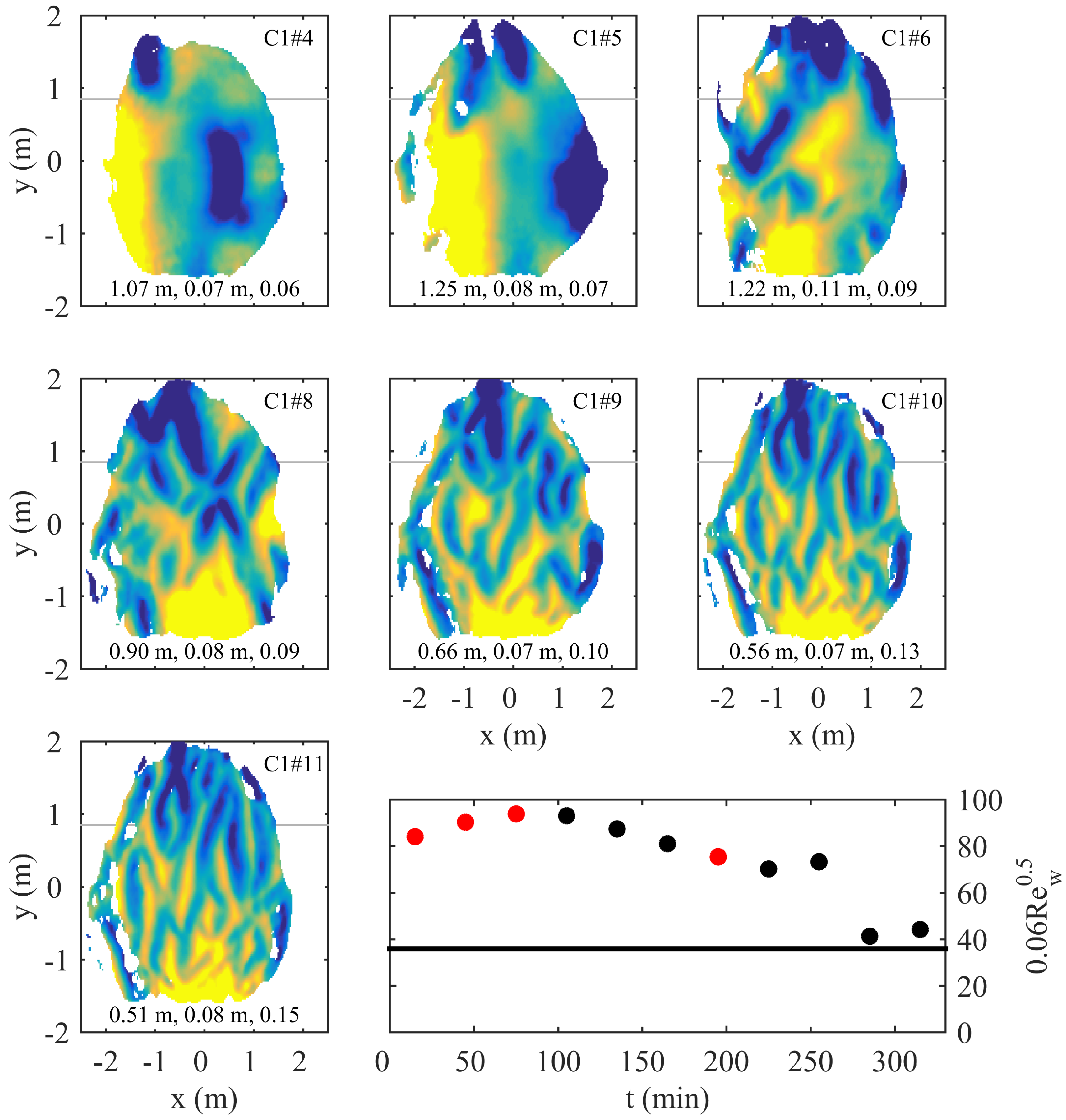
2.2.2. 3D Sonar Data

A 1.1 MHz 3D Profiling Sonar 2001 (Marine Electronics Ltd., Guernsey, UK) was mounted in a downward looking manner at x = 63 . 1 m, 1.65 m from the nearest flume wall. It was operated in two distinct modes to, firstly, obtain high-resolution circular elevation models of wave-ripple induced bed variability and hence planform geometry after a wave run and, secondly, to provide insight into cross-shore ripple migration during a wave run. In its first operation mode, the sonar was triggered manually after wave action had ceased to scan a 120 ° swath with a 0.9 ° resolution and then to rotate by 0.9 ° to capture the next swath until a complete circular area underneath the sonar was surveyed. Because the mounting height was about 1 m above the bed, the diameter of the surveyed circle was approximately 3.5 m. From each swath a bed profile was detected using a threshold algorithm. The detected bed points (typically, about 17,500) were interpolated on a regular horizontal grid with a 0.025 m spacing using l x = l y = 0 . 15 m, where l y is an alongshore scale parameter. For consistency with the processing of the cross-shore profile data, we would have liked to use l x = l y = 0 . 05 m, but this resulted in rather gappy bed elevation models, especially at the edges of the scan. All resulting models of bed elevation were subsequently detrended using the z b b ( x , t ) beneath the sonar to yield zero-mean, approximately circular models of wave-ripple induced bed variability. As in the z ˜ w r ( x ) profiles, positive and negative perturbations correspond to ripple crests and troughs, respectively. The horizontal coordinates are relative to the sonar, with positive x s onshore and negative y s to the nearest flume wall. The ripple planform geometry was classified qualitatively for each circular elevation model as 2D, quasi-2D or 3D using definitions provided in [8]. This classification is not affected by the use of l x = l y = 0 . 15 m rather than l x = l y = 0 . 05 m.
The second mode of operation was applied during a wave run. Because we expected ripple location and/or planform geometry to change during the approximate 11-min duration of a complete circular scan, we essentially applied the sonar as a 2D (cross-shore) line scanner and triggered it manually every 2 to 5 min. All cross-shore swaths were produced into cross-shore profiles of bed variability with the same threshold algorithm as used to process a full no-wave scan and were subsequently demeaned using l x = 3 . 5 m. The cross-shore ripple migration speed C r was estimated using a cross-correlation of the time-separated, zero-mean, wave-ripple induced bed profiles, e.g., [7,19,20]. The cross-shore distance over which the ripples migrated shows up as the lag with the maximum correlation.

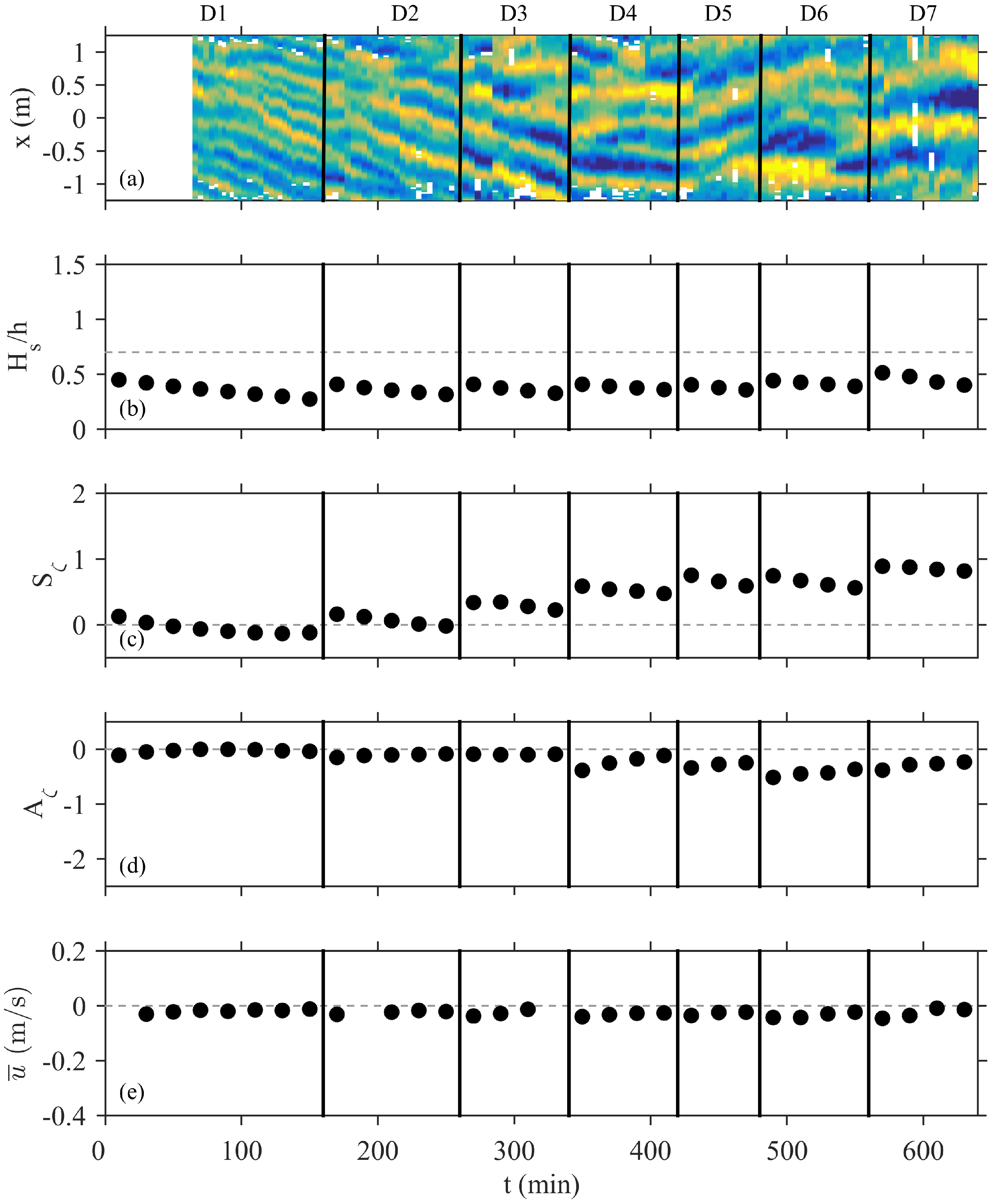
2.3. Measurements: Hydrodynamical Data

Estimates of well-established hydrodynamical parameters related to ripple characteristics and migration are available at up to 16 cross-shore locations (Figure 1). Pressure transducers were wall-mounted at all 16 locations and sampled near-bed pressure with frequencies of 4, 5 or 20 Hz depending on location. All pressure series were converted to water-surface elevation ζ series using linear wave theory, which were processed into the short-wave (0.05–2 Hz) (1) significant wave orbital diameter d s = H s / sinh ( k h ) , where H s is the local significant wave height, and k is the wave number estimated from linear theory using water depth h and the peak period T p 1 at the most seaward pressure transducer ( x = 36 . 2 m in Figure 1); (2) peak semi-orbital velocity u w = π d s / T p 1 ; (3) mobility number ψ = u w 2 / ( R g D 50 ) , (4) Shields parameter θ = 0 . 5 f w ψ , where f w is a friction factor for which we used Equations (60a) and (60b) in [35]; (5) wave Reynolds number R e w = 0 . 5 u w d s / ν ; (6) wave skewness S ζ = ζ 3 ¯ / σ ζ 3 , where the overbar represent a run average and σ ζ is the standard deviation of ζ; and, (7) wave asymmetry A ζ = H ζ 3 ¯ / σ ζ 3 , where H ζ represents the Hilbert transform of ζ. Because the paddle motion was not repeated exactly in each run, the resulting wave height and period varied slightly from run to run [36]. We therefore preferred the use of the measured peak period at the most seaward sensor T p 1 (see Table 1) over the target value T p 0 in the computation of d s and u w . Both S ζ and A ζ are measures of wave non-linearity [37]. S ζ is positive when waves have high, narrow crests and broad, shallow troughs and A ζ is negative when waves are forward-leaning. At four locations the pressure transducer was co-located with a near-bed (typically, 0.11 m above the bed) electromagnetic or acoustic current meter (Figure 1), which sampled at 4 or 10 Hz, respectively. All instantaneous time-series of cross-shore velocity were processed into the run-average cross-shore velocity u ¯ , with positive u ¯ directed landward.
Figure 4 visualizes the encountered forcing conditions. To put our ripple data in a broader perspective, the conditions of a number of other data sets are shown too. These include the field-laboratory data compiled by Goldstein et al. [6], the Sennen Beach data of Masselink et al. [7] ( D 50 = 600 μm), and the Georgia Shelf data of Nelson and Voulgaris [38] ( D 50 = 388 μm). The Bardex II data extends these earlier data sets with strong hydrodynamic conditions (large d s and u w ) for given T p and D 50 (Figure 4a–e). The wave Reynolds number ranged between 1 . 1 × 10 5 and 6 . 4 × 10 6 . When compared to the R e w conditions for the coarse-sand ripple data compiled by Pedocchi and Garcia [5] (e.g., their Figure 11a indicates 1 × 10 3 to 1 × 10 6 for R e p 40 ), this range also reflects the strong hydrodynamic conditions in our data set. Our data were collected beneath shoaling waves, breaking (plunging) waves and bores. This is also reflected by the wide range in relative wave height H s / h (≈0.3–1.5), where, based on visual observations [39], H s / h 0 . 7 delineated the shoaling from the surf zone. The Shields parameter θ increased with H s / h from 0 . 2 to 2 (Figure 4f). The orbital motion was mostly non-linear: S u ranged from 0 to about 1.5, and was typically largest where waves started to break (Figure 4g), while A ζ generally became non-zero in the wave shoaling zone and was largest (≈−2) just seaward of the swash zone (Figure 4h). The mean current u ¯ also was mostly offshore directed and ranged from 0 m/s under non-breaking waves to about 0 . 2 m/s in the surf zone (Figure 4i).
Figure 4. Visualization of the range in local forcing conditions, expressed as two-dimensional scatter plots involving the peak period T p 1 , significant wave orbital diameter d s , peak semi-orbital velocity u w , median grain size D 50 , relative wave height H s / h , Shields parameter θ, skewness S ζ , asymmetry A ζ and the mean cross-shore flow u ¯ . Brown dots: Bardex II data; grey dots: Goldstein et al. [6]; light-red dots: Masselink et al. [7]; green dots: Nelson and Voulgaris [38]. The vertical dashed line in (f)–(i) delineates the shoaling zone ( H s / h < 0 . 7 ) from the surf zone ( H s / h 0 . 7 ).
Jmse 03 01568 g004
Exploring a relationship between ripple geometry and hydrodynamical parameters demands the ripples to be in equilibrium with the hydrodynamical forcing. Based on full-scale flow tunnel experiments [40] established that the number of wave cycles to equilibrium, n e , decreases exponentially with ψ as n e = exp 0 . 036 ψ + 7 . 44 and depends little on the initial bed configuration. Most of our ψ (≈35–350) are well above the largest ψ in [40]’s data (≈55), suggesting that for our data n e is O ( 10 2 ) or less. Given the wave periods deployed during the Bardex II tests, this implies that wave runs were mostly of sufficient duration for the ripples to reach equilibrium along the entire bed profile. To avoid any non-equilibrium conditions, the ripple data collected after the first three runs of A1 and of D1 were discarded.

3. Results

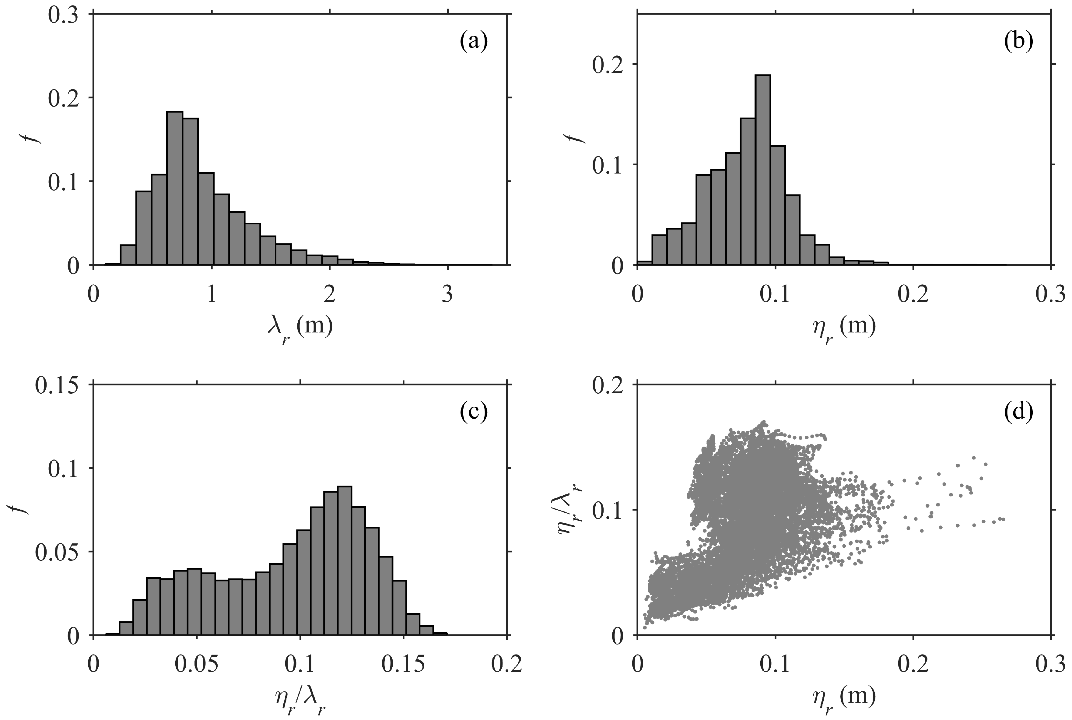
3.1. Cross-section Geometry

Examples of the cross-shore evolution of λ r , η r and ϑ r are shown in Figure 5a–c and g–i for two tests (A4 and A7) with different H s 0 and especially T p 1 and hence d s . During A4 waves started to break as plungers on the seaward edge of the sandbar ( x = 68 m; Figure 5d), while during A7 plunging commenced slightly further landward ( x = 70 75 m, Figure 5j). In both tests, λ r and d s / D 50 were approximately constant for x < 60 m, increased simultaneously to peak in the outer part of the surf zone, and then both decreased further onshore towards the beach face (compare Figure 5a,e to Figure 5g,k, respectively). Thus, the ripples were clearly orbital ripples, despite the fact that in both cases the d s / D 50 were well above the previously defined transition ( d s / D 50 = 2000 ) from orbital into suborbital ripples and even above the lower limit ( d s / D 50 = 5000 ) for anorbital ripples [11,13]. During both A4 and A7 η r was approximately constant at 0.1 m seaward of the surf zone, but decreased rapidly to a few centimetres under the plunging breakers, especially in test A7. During all wave runs ϑ r was approximately 0.15 over the deeper horizontal part of the flume, indicating the presence of vortex ripples, and slightly decreased to ≈0.1 at the landward edge of the shoaling zone. Inside the surf zone the ripples became much more subdued, with ϑ r = 0.02–0.03 in the most landward windows for which ripple geometry could be computed. Finally, we note that η r and ϑ r for a given d s / D 50 inside the surf zone were lower than for the same d s / D 50 outside the surf zone. For example, during A4 η r and ϑ r amounted to about 0.06 m and 0.05, respectively, at x = 82 m ( d s / D 50 6 , 500 ), while the ripples were higher ( η r 0 . 09 m) and steeper ( ϑ r 0 . 10 ) at x = 62 . 5 m despite similar d s / D 50 . This difference seems to be substantially less for λ r .
The temporal evolution of λ r , η r and ϑ r is shown in Figure 6a–c for two example locations ( x = 55 and 80 m), together with the local values of H s / h , d s / D 50 and θ (Figure 6d–f, respectively). The seaward ( x = 55 m) location was near the seaward end of the steep sloping profile (Figure 1) and always experienced non-breaking wave conditions (Figure 6d, H s / h < 0 . 7 ), while waves at the shallower landward location ( x = 80 m) waves could either be shoaling or breaking depending on H s 0 , T p 1 , h s and the sandbar morphology. Temporal variability in H s / h , d s / D 50 and θ mostly reflected changes in H s 0 , T p 1 or h s . For example, d s / D 50 and θ increased step-wise between tests in series D because of an increase in peak period T p 1 and reduced slightly within a test because of an increase in the still water level h s (Table 1). Also note the “tidal” signal in the wave conditions during tests C1 and C2. The gradual reduction in H s / h , d s / D 50 and θ during A6 at x = 80 m was induced by the increase in local water depth associated with onshore sandbar migration. The wider range in wave conditions at x = 80 m is also reflected in a wider range in the cross-section ripple characteristics. Especially series C and D showed a clear positive dependence of λ r on d s / D 50 (compare Figure 6a and Figure 6e). This is consistent with the suggestion based on Figure 5 that the ripples were orbital, even though again d s / D 50 extended well into the previously defined d s / D 50 -space of anorbital ripples. Under non-breaking conditions η r also increased with d s / D 50 , resulting in an approximately constant ϑ r of 0.1–0.15 (vortex ripples; Figure 6c). Clearly, the ripples were substantially less pronounced under breaking waves, with a clear reduction in ϑ r with θ (compare Figure 6c and Figure 6f).
Figure 5. Cross-shore profiles of (a) ripple length λ r ; (b) ripple height η r ; (c) ripple steepness ϑ r ; (d) significant wave height H s and (e) normalized orbital diameter d s / D 50 for all five runs in test A4. Panel (f) shows the corresponding bed profiles. Panels (g)–(l) are the same as (a)–(f) but for test A7. The two horizontal lines in (e) and (k) are previously defined values ( d s / D 50 = 2000 and 5000; [11,13]) to delineate the orbital, suborbital and anorbital ripple regimes. The horizontal blue line in (f) and (l) is the still water level h s = 3 m. The colors in all panels represent the different runs.
Jmse 03 01568 g005
Figure 6. Temporal evolution of (a) ripple length λ r ; (b) ripple height η r ; (c) ripple steepness ϑ r ; (d) relative wave height H s / h ; (e) normalized orbital diameter d s / D 50 and (f) Shields parameter at x = 55 (black dots) and 80 m (red dots). The cross-section ripple data in (a)–(c) are based on a 10-m wide window centered at each x. The vertical grey lines in each panel mark the transition between tests. Note that the horizontal axis corresponds to the cumulative number of wave runs. Because runs were of different duration, the horizontal axis is not equidistant with time. The horizontal line in (d) marks the approximate transition between non-breaking and breaking conditions ( H s / h = 0 . 7 ). The two horizontal lines in (e) are previously defined values ( d s / D 50 = 2000 and 5000; [11,13]) to delineate the orbital, suborbital and anorbital ripple regimes. No values at x = 80 m are shown in (d)–(f) for B2 and for several C1 and C2 wave runs because the instrument was not submerged continuously during these low h s runs.
Jmse 03 01568 g006
Figure 7a illustrates that λ r normalized by D 50 did indeed not follow the orbital-suborbital-anorbital trend with d s / D 50 found in fine-grained sand, where here this trend is indicated by the empirical predictor of Nelson et al. [4]. Instead, the trend is a growth in λ / D 50 with d s / D 50 over the entire d s / D 50 range in the data, implying all our large coarse-grained wave ripples to be orbital ripples. It is, however, also obvious from Figure 7a that the ratio of λ r to d s was less than 0.65, a typical value quoted for orbital ripples. What is more, λ r / d s reduced with d s from about 0.55 for d s / D 50 1400 to about 0.27 for d s / D 50 11 , 500 , in contrast to earlier laboratory observations [8] that indicated λ r / d s to be constant for given D 50 . The λ r / d s values quoted here were obtained by averaging λ / D 50 in 0.1 wide log 10 d s / D 50 bins. Unsurprisingly, η r / D 50 did not follow the anorbital trend with d s / D 50 for d s / D 50 > 5000 (Figure 7b). As for λ r , the proportionality between η r and d s decreased with d s , from about 0.08 for d s / D 50 1400 to about 0.02 for d s / D 50 > 8000 . The scatter in the observations near d s / D 50 6000–8000 is substantial. This is caused by the occurrence of these d s / D 50 values both inside and outside the surf zone with, as illustrated with Figure 5, substantially different η r . Figure 7c demonstrates the expected change from vortex ripples ( ϑ r 0 . 1 0 . 15 ) for low d s / D 50 (here, d s / D 50 5000 ) to more subdued ripples at high d s / D 50 , although the scatter is again appreciable. We compare measured λ r , η r and ϑ r to empirical predictors of ripple geometry designed for orbital ripples over the full d s / D 50 range in Section 4.
Figure 7. Measured (a) ripple length λ r and (b) ripple height η r , normalized by the median grain size D 50 , and (c) ripple steepness ϑ r versus normalized orbital diameter d s / D 50 , based on all observations at the 16 instrumented locations (1687 observations in total). The two vertical lines in all three panels are previously defined values ( d s / D 50 = 2000 and 5000; [11,13]) to delineate the orbital, suborbital and anorbital ripple regimes. The curved black line in each plot represents the empirical predictor of Nelson et al. [4] to illustrate expected orbital-suborbital-anorbital trends in λ r / D 50 , η r / D 50 and ϑ r , respectively. The red sloping lines in (a)–(c) are λ r / D 50 = 0 . 65 , η r / D 50 = 0 . 10 and ϑ r = 0 . 15 , values often quoted for orbital vortex ripples. The brown dots in each panel are average values computed from the measurements for 0.1-wide log 10 d s / D 50 bins.
Jmse 03 01568 g007

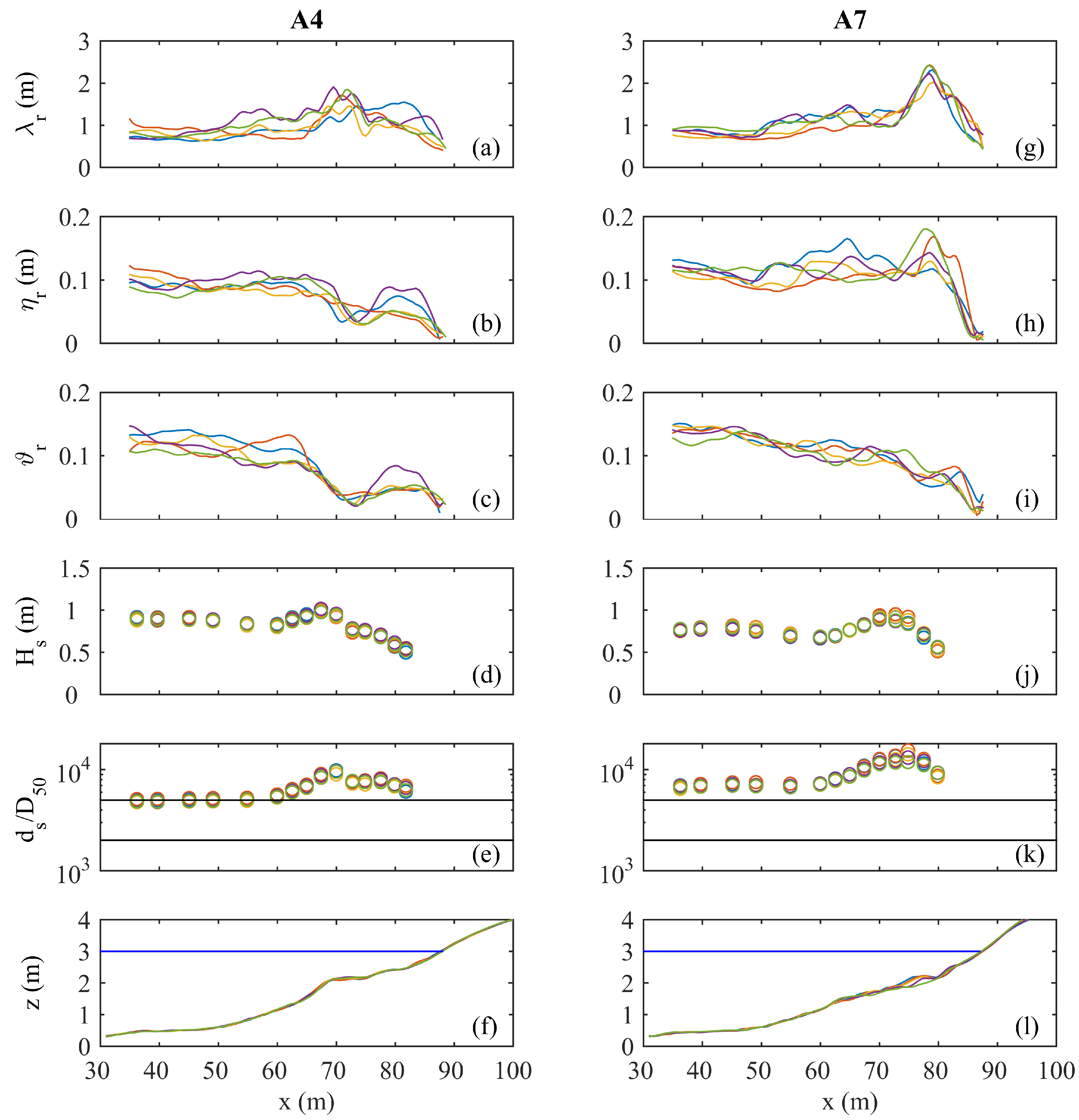
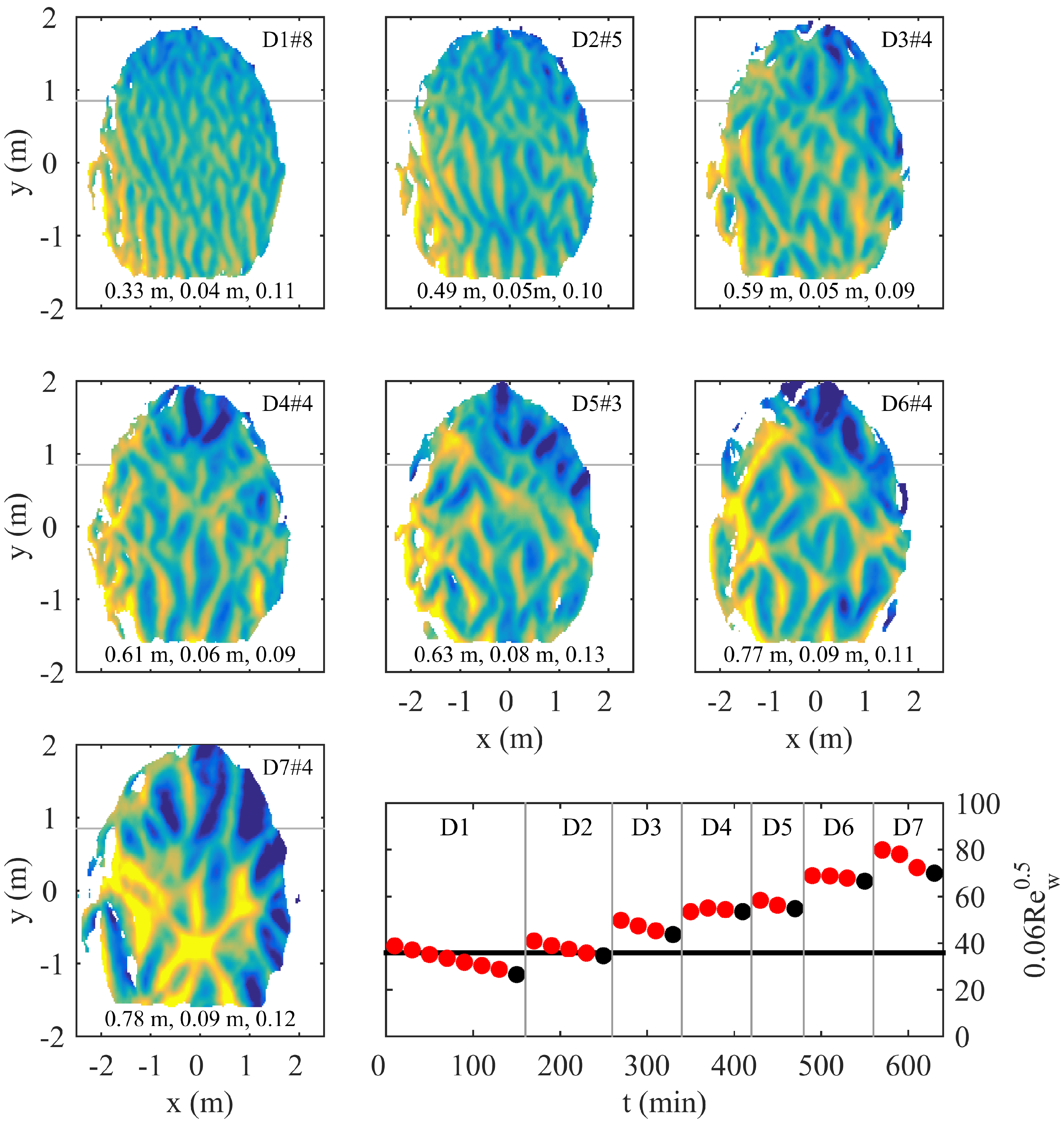
3.2. Planform Geometry

None of the bed elevation models collected at x = 63 . 1 m revealed two-dimensional ripples with straight, uniform crests perpendicular to the wave direction that are characteristic of the coarse-grained wave ripples in existing field, e.g., [21,22,23,26], and several laboratory settings [8,28]. Instead, all models showed quasi two-dimensional to highly three-dimensional planform geometries. We illustrate this for series D and test C1 in Figure 8 and Figure 9, respectively. In both figures the flow conditions are expressed as 0 . 06 R e w 0 . 5 , because [5] illustrated that ripples become two-dimensional for R e p > 0 . 06 R e w 0 . 5 and are three-dimensional otherwise. At the end of test D1, when 0 . 06 R e w 0 . 5 was below R e p and at its lowest at x = 63 . 1 m for the entire Bardex II experiment, the ripples were quasi two-dimensional: ripple crests were reasonably continuous (sometimes up to several metres) and the crest-to-crest distance along two adjacent ripples was, at least visually, fairly constant, but the crests varied in orientation and some had notably variations in height. Also, some ripples bifurcated and several defects can be seen. With an increase in 0 . 06 R e w 0 . 5 to about 65 (i.e., well above R e p ), this planform changed gradually into oval mounds to which ripples with remarkably different orientations were attached (D6 and D7). This planform geometry was also observed during test C1 when 0 . 06 R e w 0 . 5 was about 75 (i.e., runs 8 and 9 in Figure 9). For 0 . 06 R e w 0 . 5 > 80 in test C1 (runs 4, 5 and 6 in Figure 9; the highest values observed at x = 63 . 1 m), the bed contained large, three-dimensional and gentle ( ϑ r 0 . 07 ) highs and lows only, closely resembling hummocky bed forms in fine-sand laboratory experiments [8,41,42,43] and field conditions [44]. For smaller 0 . 06 R e w 0 . 5 in test C1 (runs 10 and 11 in Figure 9), the ripples became quasi two-dimensional, similar in appearance to that observed in tests D1 and D2 (Figure 8). The hydrodynamic forcing never became sufficiently energetic at x = 63 . 1 m to reach flat bed conditions. Cross-shore profiles of ϑ r suggest that such conditions were reached only in the swash zone on the beach face (Figure 5c,i). Although we do not have bed elevation models for 0 . 06 R e w 0 . 5 well below R e p , our data confirm Pedocchi and Garcia [5]’s findings that ripple planform geometry is related to the wave Reynolds number and that 0 . 06 R e w 0 . 5 = R e p is a reasonable threshold above which ripples are three-dimensional.
The succession of equilibrium planform geometry for coarse sand that thus follows from Figure 8 and Figure 9 for 0 . 06 R e w 0 . 5 > 25 is a transition from quasi two-dimensional ripples, through oval mounds with ripples attached from different directions, to three-dimensional hummocky bed forms. This change in planform is also associated with an increase in λ r and hence, as deduced from Figure 7a, a reduction in λ r / d s . In other words, the strongly three-dimensional ripples in our data set generally had lower λ r / d s than the more moderately three-dimensional or quasi two-dimensional ripples. As an illustration, λ r / d s was near 0.3 for the strongly three-dimensional ripples in D7 and D8, and about 0.5 for the quasi two-dimensional ripples in D1. The dependence of λ r / d s on ripple planform observed here is qualitatively consistent with previous field [24] and laboratory [28] observations.
Figure 8. Bed elevation models for selected tests and runs during series D. Warm (yellow) colours are ripple crests, cold (blue) colours are ripple troughs. The colors range from 0 . 08 to 0 . 08 m. DX#Y stands for run Y in test DX. The local x and y coordinates are relative to the sonar, with ( x , y ) = ( 0 , 0 ) vertically below the sonar, and with x positive onshore. The local x = 0 m corresponds to x = 63 . 1 m in Figure 1. The nearest flume wall is at y = 1 . 65 m. The 3 numbers at the bottom of each panel are the ripple wavelength λ r , height η r and steepness ϑ r based on the profile data. The center line of the flume is indicated by the gray line. The forcing conditions are expressed as a time series of 0 . 06 R e w 0 . 5 ; time t = 0 is the start of series D. The horizontal black line is the particle Reynolds number R e p . The black dots represent the times of the shown bed elevation models.
Jmse 03 01568 g008
Figure 9. Bed elevation models for selected runs in test C1. For additional explanation, see the caption of Figure 8. Here, time t = 0 is the start of test C1. During test C1 0 . 06 R e w 0 . 5 reduced by a decrease in the still water level h s and in the last two runs by a decrease in the significant wave height H s 0 (Table 1).
Jmse 03 01568 g009
The five consecutive bed elevation models in test A4 (Figure 10) clearly document that the three-dimensional ripples shifted and changed perpetually under approximately constant hydrodynamical forcing (Figure 5d,e). Yet, their average size ( λ r and η r ) remained fairly constant, see also Figure 5a–c. Ripple migration, separation and amalgamation seem to have taken place continuously, although it is difficult to tell how individual bed forms actually evolved within a run. Comparable dynamics were also observed during all other tests in series A and B (not shown). Similar to fine-grained three-dimensional ripples, e.g., [27,42,45], the coarse-grained three-dimensional ripples in our data thus exhibited dynamic-equilibrium behaviour.
Figure 10. Bed elevation models for all five runs in test A4. For additional explanation, see the caption of Figure 8. Here, time t = 0 is the start of test A4.
Jmse 03 01568 g010

3.3. Ripple Migration

Spatially and temporally coherent ripple migration was discernable at the sonar location only when the planform geometry was classified as quasi two-dimensional. This was, as illustrated in Figure 11a, the case for tests D1–D3. Ripple migration was found to be offshore directed and to amount to about 0.01 m/min. During these tests S ζ and A ζ were both close to 0 (Figure 11c,d) and u ¯ was weak ( 0 . 03 m/s or less, see Figure 11e), representative of conditions well seaward of the surf zone (Figure 4 and Figure 11b). This would indicate that neither wave non-linearity nor the current are driving the ripple migration. Instead, the offshore ripple migration presumably reflects downslope gravity-induced bedload transport. This would corroborate numerical sand transport computations [33,46] that demonstrate downslope gravity-induced transport to be a significant contributor to the total sand transport on the present steep profile under non-breaking wave conditions.
For the more energetic D4–D7 tests the individual ripples could simultaneously migrate landward or seaward, or not migrate at all (Figure 11a). In a few cases a ripple changed migration direction (e.g., D7, the ripple between x 0 . 5 and 1 . 0 m) or split into two parts (e.g., near the end of D6 at x 0 . 75 m) during a test. In addition, two ripples could merge (e.g., near the end of D6 at x 0 . 25 m). Similar observations were made during all tests in which the ripple planform resembled oval mounds with ripples attached from different directions (not shown). The now rather large (and positive) S ζ (Figure 11c) is obviously not associated with coherent onshore bedform migration as found previously for two-dimensional orbital wave ripples [24,25] and for anorbital [47] and subdued large wave ripples [19] in finer sand. The present spatially and temporally incoherent pattern expresses the dynamic-equilibrium behaviour of the ripples, including ripple separation and amalgamation.
Figure 11. (a) Time-space diagram of wave-ripple induced bed variability beneath the sonar during series D. Warm (yellow) colours are ripple crests, cold (blue) colours are ripple troughs. The colors range from 0 . 05 to 0 . 05 m. The cross-shore coordinate is relative to the sonar, with x = 0 vertically below the sonar, and with positive x onshore. The local x = 0 m corresponds to x = 63 . 1 m in Figure 1. Time series of (b) the relative wave height H s / h , (c) skewness S ζ , (d) asymmetry A ζ and (e) the mean cross-shore flow u ¯ . In (b)–(e) the limits of the vertical axis were set to equal to the range in the entire data set, see Figure 4. H s / h , S ζ and A ζ were measured at x = 62 . 5 m, u ¯ at x = 65 m. The dashed line in (b) marks the approximate H s / h transition between non-breaking and breaking waves.
Jmse 03 01568 g011

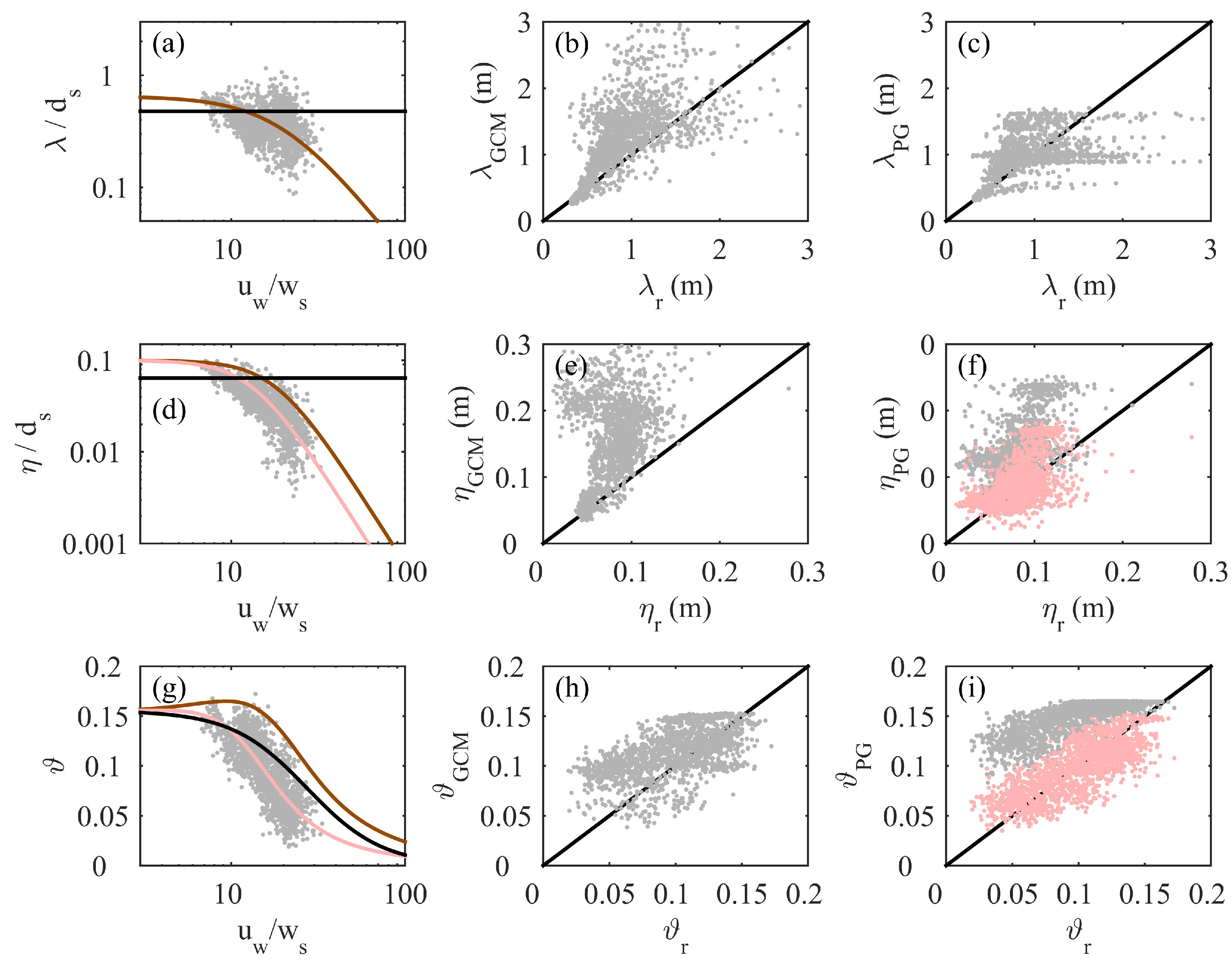
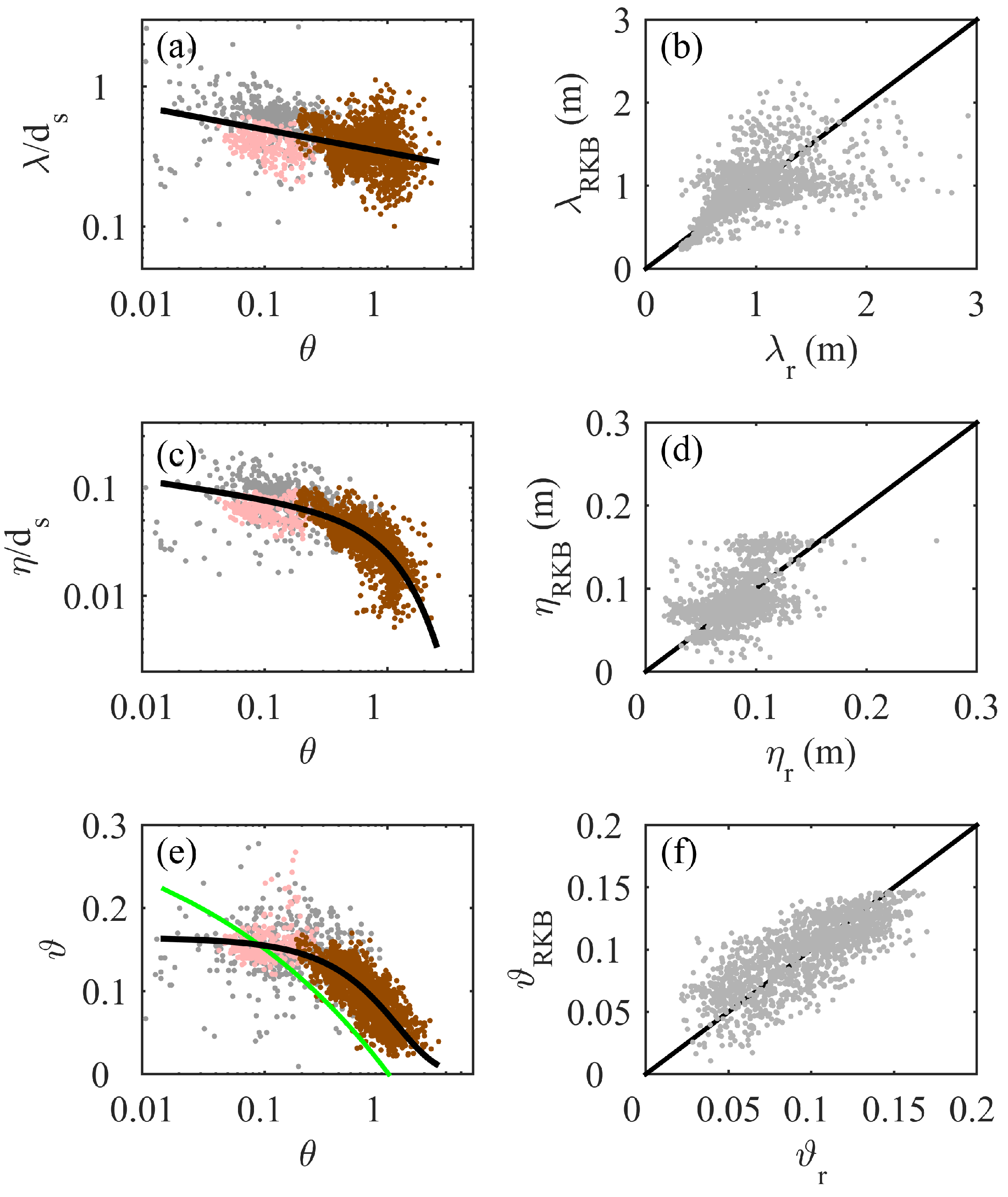
4. Empirical Prediction

The persistent orbital-nature of coarse-sand wave ripples precludes the use of empirical predictors that produce orbital-suborbital-anorbital trends in λ r and η r , e.g., [4,11]. Therefore, we now test the orbital Goldstein et al. [6] (henceforth GCM) and the coarse-sand Pedocchi and Garcia [5] (henceforth PG) predictors against our data (Figure 12). The GCM predictors are based on a compilation of laboratory and field data sets from which suborbital and anorbital ripples were discarded when they were superimposed on large wave ripples, and retained anorbital ripples were additionally removed for u w / w s 25 . Using genetic programming Goldstein et al. [6] obtained the following predictors
λ GCM / d s = 1 1 . 12 + 2 . 18 D 50
η GCM / d s = 0 . 313 D 50 1 . 12 + 2 . 18 D 50
ϑ GCM = 3 . 42 22 + λ GCM / D 50 2
Figure 12. Measured (a) normalized ripple length λ r / d s , (d) normalized ripple height η r / d s and (g) ripple steepness ϑ r versus the ratio of the peak semi-orbital velocity u w over the sediment fall velocity w s (gray dots). The black and brown lines in (a), (e) and (g) are the GCM and PG predictors, respectively; in (g), T p = 8 s was used to relate u w to d s in the GCM predictor. Other panels are scatter plots of predicted against measured ripple parameters together with the 1:1 line. The light-red lines in (d) and (g), and the light-red dots in (f) and (i) correspond to the modified PG η / d s predictor, see text for further explanation.
Jmse 03 01568 g012
For a given D 50 λ GCM and η GCM thus scale linearly with d s (i.e., orbital ripples). The present D 50 = 430 μm results in λ GCM / d s = 0 . 49 and η GCM / d s = 0 . 065 (Figure 12a,d, respectively). The PG predictors are also based on laboratory and field data sets, from which PG discarded the characteristics of the large wave ripples when they were overlain by suborbital or anorbital ripples. PG related ripple dimensions to the ratio u w / w s as
λ PG / d s = 0 . 65 0 . 050 u w / w s 2 + 1 1
η PG / d s = 0 . 1 0 . 055 u w / w s 3 + 1 1
and ϑ PG = η PG / λ PG . In contrast to the GCM predictors, the ratios λ PG / d s and η PG / d s are not constant for a given D 50 , but decrease with u w (Figure 12a,d). For u w / w s < 10 , ϑ PG is about constant near 0.16 and then decreases to < 0 . 05 for u w / w s > 50 (Figure 12g). Three error measures were computed to quantify the performance of the two predictors for λ r , η r and ϑ r : the bias b, the root-mean-square error ϵ rms , and the correlation-coefficient squared r 2 of the best-fit linear line between a predicted and measured ripple parameter. Both b and ϵ rms were normalized by the range of the observed values for each parameter predicted:
b = 1 N X p X m max X m min X m
and
ϵ rms = 1 N X p X m 2 max X m min X m
where X is the evaluated parameter, the subscripts p and m denote predicted and measured values, respectively, and N is the total number of observations. All error statistics are listed in Table 2.
Table 2. Equilibrium predictor error statistics.
GCM PG RBK
λ r η r ϑ r λ r η r ϑ r λ r η r ϑ r
b0.110.340.100.020.230.320.000.020.01
ϵ rms 0.170.430.200.120.270.350.130.110.13
r 2 0.360.070.320.210.300.580.330.290.61
The constant values for the ratios λ GCM / d s and η GCM / d s are inconsistent with our data (Figure 7a,b, and Figure 12a,d), and the GCM predictors overestimate λ r , η r , and ϑ r substantially (Figure 12b,e,h), with bias values of 0.11, 0.33 and 0.10, respectively. While the PG predictor produces λ / d s values that are roughly accurate, Figure 12a casts substantial doubt on the suitability of u w / w s to predict the trend in λ / d s . For u w / w s < 20 , most λ r / d s are lower than predicted, while the opposite is true for larger u w / w s . As a consequence, the overall agreement between λ PG and λ r is low (Figure 12c), with r 2 = 0 . 21 only. The η r / d s does decrease with u w / w s , but predicted values are substantially larger (Figure 12d). As a consequence, the bias values for η PG and ϑ PG are large (0.23 and 0.32, respectively). This systematic difference can be removed largely by modifying Equation (5) into
η PG / d s = 0 . 1 0 . 075 u w / w s 3 + 1 1
This modified predictor is shown with the light-red lines in Figure 12d,g, and corresponding dots in Figure 12f,i. Although this change results in near-zero bias, the r 2 for η PG remains low (0.27); for ϑ PG the r 2 is substantially higher (0.61).
The overall poor performance of the GCM and PG predictors motivated us to design alternative predictors for the equilibrium length, height and steepness of coarse-grained wave ripples. To this end, we combined our Bardex II data with all equilibrium ripple data from the Goldstein et al. [6] database with D 50 300 μm and the Sennen Beach data of Masselink et al. [7]. A scatter plot of observed λ / d s versus the Shields parameter θ (Figure 13a) suggest that log 10 λ / d s = a 0 + a 1 log 10 θ , where a 0 and a 1 are fit parameters, is a meaningful predictor. A least-squares fit resulted in a 0 = 0 . 471 ± 0 . 008 and a 1 = 0 . 163 ± 0 . 014 , where the ±value provides the 95% confidence range. This fit can be rewritten into
λ RBK / d s = 0 . 338 θ 0 . 163
Our fit, indicated by the subscript RBK, thus results in a reduction of λ / d s from 0.55 at θ = 0 . 05 to 0.3 at θ = 2 . The dependence of ϑ on θ (Figure 13e) suggests a predictor of the form ϑ = a 2 a 2 tanh a 3 θ a 4 , where a 2 to a 4 are fit parameters. A least-squares fit resulted in a 2 = 0 . 164 ± 0 . 004 , a 3 = 0 . 630 ± 0 . 020 and a 4 = 1 . 038 ± 0 . 080 . Thus,
ϑ RBK = 0 . 164 0 . 164 tanh 0 . 630 θ
considering that the 95% confidence band of a 4 encompasses 1. This fit produces ϑ 0 . 15 for θ < 0 . 2 and a subsequent reduction in ϑ to 0.02 for θ = 2 . We note that an earlier θ-based predictor for ripple steepness was proposed in Nielsen [48], ϑ = 0 . 342 0 . 34 θ 4 . It is obvious from Figure 13e that this fit is not a good approximation of the present combined data set. Finally, the normalized ripple height, η RBK / d s , can be computed for a given θ as the product of λ RBK θ and ϑ RBK θ (Figure 13c). This results in η R B K / d s 0 . 1 for low θ and a reduction in η R B K / d s with θ to η R B K / d s < 0 . 01 for θ > 1 . 5 .
The application of our fits to the Bardex II ripple data only (Figure 13b,d,f) results in improved error statistics compared to the GCM and PG predictors (Table 2), with near-zero bias and reduced root-mean-square error, the latter in particular for η r and ϑ r . Figure 13b illustrates that the differences between λ R B K and λ r are most pronounced for large λ r and can amount to 1 m or more. A closer inspection of these differences revealed that they are largest for the H s / h = 0 . 6 1 . 0 range, that is, in the outer surf zone where the waves broke as plungers. Vortices in plunging breakers are known to penetrate into the water column, e.g., [49,50] and, upon impact with the bed, to forcefully lift sand into suspension, e.g., [51,52,53]. It is feasible that this modifies ripple geometry and explains, at least partly, the generally poor agreement between predicted and observed ripple lengths. It would also explain why non-filtered ripple length estimates scatter most on the sandbar (Figure 2). For lower H s / h the waves are non-breaking, while for larger H s / h the plunging waves have evolved into bores in which breaking-induced turbulence near the bed is less intense and wave ripples are presumably again determined largely by the near-bed orbital flow.
Figure 13. Measured (a) normalized ripple length λ / d s , (c) normalized ripple height η / d s and (e) ripple steepness ϑ versus the Shields parameter θ. Brown dots: Bardex II data; grey dots: Goldstein et al. [6]; light-red dots: Masselink et al. [7]. The black lines are our least-squares fits based on all data. The green line in (e) is based on Nielsen [48]. Panels (b), (d) and (f) are scatter plots of predicted versus measured ripple parameters (Bardex II data only) together with the 1:1 line.
Jmse 03 01568 g013

5. Discussion

In this paper we have extended earlier work on coarse-grain wave ripples by exploring their characteristics under full-scale, irregular waves with large orbital motion (Figure 4). The data illustrated that the ripples are orbital for the entire range of d s / D 50 encountered (≈1000–20,000), with a reduction in the ratios λ r / d s and η r / d s with increasing d s / D 50 (Figure 7a,b). Simultaneously, the ripple steepness reduced from 0.1–0.15 (vortex ripples) to <0.05 (Figure 7c), and the planform geometry changed from quasi two-dimensional ripples to strongly three-dimensional hummocky bed forms under the most energetic conditions (Figure 8 and Figure 9). In other words, coarse-grain ripples can become three-dimensional when the wave forcing is sufficiently strong and wave-formed hummocks are not restricted to fine sands.
We realize that by deriving Equations (9) and (10) we have added yet another predictor to the existing plethora of equilibrium ripple predictors. For mild wave conditions ( d s / D 50 < 2000 ) most predictors, including ours, produce orbital vortex ripples with λ r / d s 0 . 65 , η r / d s 0 . 1 and ϑ r 0 . 15 . For more energetic conditions our predictor produces cross-section ripple characteristics that deviate considerably from suborbital-anorbital trends. Field data sets, e.g., [17,19,20], have shown suborbital or anorbital ripples up to about D 50 = 300 μm. Accordingly, we propose that our predictor should be used only when D 50 exceeds 300 μm. This is larger than Pedocchi and Garcia [5]’s definition of coarse sand; their R e p 13 corresponds to ≥220 μm (quartz sand) at 20 o C. For finer sand we recommend the use of the Nelson et al. [4] predictor as it is based on a vast amount of data and outperforms many other predictors. This implies that, as [5], we advocate the use of grain size dependent predictors. This has the disadvantage of potential spatial discontinuities in predictions of cross-section ripple geometry when spatially explicit grain size maps are used as input in hydrodynamic and morphodynamic models. We do not know whether there is a need to include a third, intermediate grain size predictor to, for example, minimize the discontinuities. This will depend on the width of the grain size range into which ripple type changes with increasing orbital flow from orbital-suborbital-anorbital into orbital only. New laboratory experiments, for instance in a large oscillating water tunnel, using sands with D 50 ranging from ≈250 μm to ≈350 μm under mild, intermediate and high orbital flow may shed further light on this issue and will aid in providing a physical explanation for the change in ripple behaviour with flow conditions near 300 μm.

6. Conclusions

Wave-formed ripples with equilibrium length λ r = 0 . 31 2 . 38 m, height η r = 0 . 01 0 . 17 m and steepness ϑ = 0 . 01 0 . 16 were observed in the shoaling and surf zone of a coarse sand, prototype laboratory beach under a range of wave conditions and water depths. Our data confirm findings from earlier limited laboratory data that coarse-grained wave ripples remain orbital, even when the ratio of orbital diameter to median grain size d s / D 50 is in the part of parameter space where in fine sand anorbital ripples form. The ratio of λ r to d s is not constant, but decreases from about 0.55 for d s / D 50 1400 to about 0.27 for d s / D 50 11 , 500 . Analogously, ripple height η r increases with d s , but the proportionally decreases from about 0.08 for d s / D 50 1400 to about 0.02 for d s / D 50 > 8000 . Ripple planform geometry changes with increasing wave Reynolds number from vortex ripples with wavy crests, through oval mounds with ripples attached from different directions, to strongly subdued hummocky features. Our data thus indicate that coarse-grained wave ripples can be three-dimensional if the orbital flow is sufficiently strong and that wave-formed hummocks are not restricted to fine sands. The three-dimensional ripples show dynamic-equilibrium behaviour with ripple amalgamation and separation, but without clear onshore migration even though the orbital motion is positively (onshore) skewed and mean currents are weak. Finally, we propose new empirical equilibrium ripple predictors for D 50 > 300 μm, in which λ r / d s , η r / d s and ϑ r are a function of the Shields parameter θ. For finer sand we recommend a predictor that follows the orbital-suborbital-anorbital trend in cross-section geometry, such as that of Nelson et al. [4].

Acknowledgments

Bardex II was supported by the European Community’s 7th Framework Programme through the grant to the budget of the Integrating Activity HYDRALAB IV, contract No. 261520. The academic lead of the project was Gerd Masselink and the Deltares coordinator was Guido Wolters. Winnie de Winter, Daan Wesselman and Florent Grasso contributed significantly to the data collection, and Marcel van Maarseveen, Henk Markies and all Deltares Delta flume staff provided excellent technical support. Gerd Masselink and Evan Goldstein provided the additional ripple data sets. G.R. and J.A.B. were funded by the Dutch Technology Foundation STW, which is part of the Netherlands Organisation for Scientific Research (NWO), and which is partly funded by the Ministry of Economic Affairs (project number 12397). All data are available from the first author upon request.

Author Contributions

The authors contributed in the following proportions to design and data collection, data processing, analysis and conclusions, and manuscript preparation, respectively: G.R. (100%, 50%, 60%, 60%), J.A.B. (0%, 50%, 30%, 20%) and M.G.K. (0%, 0%, 10%, 20%).

Conflicts of Interest

The authors declare no conflict of interest.

References

  1. Van Rijn, L.C.; Walstra, D.J.R.; Grasmeijer, B.; Sutherland, J.; Pan, S.; Sierra, J.P. The predictability of cross-shore bed evolution of sandy beaches at the time scale of storms and seasons using process-based profile models. Coast. Eng. 2003, 47, 295–327. [Google Scholar] [CrossRef]
  2. Van Rijn, L.C.; Walstra, D.J.R.; van Ormondt, M. Unified view of sediment transport by currents and waves. IV: Application of morphodynamic model. J. Hydraul. Eng. 2007, 133, 776–793. [Google Scholar] [CrossRef]
  3. Ganju, N.K.; Sherwoord, C.R. Effect of roughness formulation on the performance of a coupled wave, hydrodynamic, and sediment transport model. Ocean Model. 2010, 33, 299–313. [Google Scholar] [CrossRef]
  4. Nelson, T.R.; Voulgaris, G.; Traykovski, P. Predicting wave-induced ripple equilibrium geometry. J. Geophys. Res. 2013, 118, 3202–3220. [Google Scholar] [CrossRef]
  5. Pedocchi, F.; Garcia, M.H. Ripple morphology under oscillatory flow: 1. Prediction. J. Geophys. Res. 2009, 114, C12014. [Google Scholar] [CrossRef]
  6. Goldstein, E.B.; Coco, G.; Murray, A.B. Prediction of wave ripple characteristics using genetic programming. Cont. Shelf Res. 2013, 71. [Google Scholar] [CrossRef]
  7. Masselink, G.; Austin, M.J.; O’Hare, T.J.; Russell, P.E. Geometry and dynamics of wave ripples in the nearshore zone of a coarse sandy beach. J. Geophys. Res. 2007, 112, C10022. [Google Scholar] [CrossRef]
  8. Cummings, D.I.; Dumas, S.; Dalrymple, R.W. Fine-grained versus coarse-grained wave ripples generated experimentally under large-scale oscillatory flow. J. Sediment. Res. 2009, 79, 83–93. [Google Scholar] [CrossRef]
  9. Clifton, H.E. Wave-formed sedimentary structures: A conceptual model. In Beach and Nearshore Sedimentation, Special Publication 24; Society for Sedimentary Geology: Tulsa, OK, USA, 1976; pp. 126–148. [Google Scholar]
  10. Miller, M.C.; Komar, P.D. Oscillation sand ripples generated by laboratory apparatus. J. Sediment. Res. 1980, 50, 173–182. [Google Scholar]
  11. Wiberg, P.L.; Harris, C.K. Ripple geometry in wave-dominated environments. J. Geophys. Res. 1994, 99, 775–789. [Google Scholar] [CrossRef]
  12. Van der Werf, J.J.; Doucette, J.S.; O’Donoghue, T.; Ribberink, J.S. Detailed measurements of velocities and suspended sand concentrations over full-scale ripples in regular oscillatory flow. J. Geophys. Res. 2007, 112, F02012. [Google Scholar] [CrossRef]
  13. Clifton, H.E.; Dingler, J.R. Wave-formed structures and paleoenvironmental reconstruction. Mar. Geol. 1984, 60, 165–198. [Google Scholar] [CrossRef]
  14. Maier, I.; Hay, A.E. Occurrence and orientation of anorbital ripples in near-shore sands. J. Geophys. Res. 2009, 114. [Google Scholar] [CrossRef]
  15. Soulsby, R.L.; Whitehouse, R.J.S.; Marten, K.V. Prediction of time-evolving sand ripples in shelf seas. Cont. Shelf Res. 2012, 38, 47–62. [Google Scholar] [CrossRef]
  16. Hanes, D.M.; Alymov, V.; Chang, Y.S.; Jette, C. Wave-formed sand ripples at Duck, North Carolina. J. Geophys. Res. 2001, 106, 22575–22592. [Google Scholar] [CrossRef]
  17. Grasmeijer, B.T.; Kleinhans, M.G. Observed and predicted bed forms and their effect on suspended sand concentrations. Coast. Eng. 2004, 51, 351–371. [Google Scholar] [CrossRef]
  18. Williams, J.J.; Bell, P.S.; Thorne, P.D. Unifying large and small wave-generated ripples. J. Geophys. Res. 2005, 110, C02008. [Google Scholar] [CrossRef]
  19. Miles, J.R.; Thorpe, A.; Russell, P.; Masselink, G. Observations of bedforms on a dissipative macrotidal beach. Ocean Dyn. 2014, 64, 225–239. [Google Scholar] [CrossRef]
  20. Larsen, S.M.; Greenwood, B.; Aagaard, T. Obervations of megaripples in the surf zone. Mar. Geol. 2015, 364. [Google Scholar] [CrossRef]
  21. Forbes, D.L.; Boyd, R. Gravel ripples on the inner Scotian shelf. J. Sediment. Petrol. 1987, 57, 46–54. [Google Scholar]
  22. Hunter, R.E.; Dingler, J.R.; Anima, R.J.; Richmond, B.M. Coarse-sediment bands on the inner shelf of Southern Monterey Bay, California. Mar. Geol. 1988, 80, 81–98. [Google Scholar] [CrossRef]
  23. Leckie, D. Wave-formed, coarse-grained ripples and their relationship to hummocky cross-stratification. J. Sediment. Petrol. 1988, 58, 607–622. [Google Scholar] [CrossRef]
  24. Traykovski, P.; Hay, A.E.; Irish, J.D.; Lynch, J.F. Geometry, migration, and evolution of wave orbital ripples at LEO-15. J. Geophys. Res. 1999, 104, 1505–1524. [Google Scholar] [CrossRef]
  25. Doucette, J.S. Bedform migration and sediment dynamics in the nearshore of a low-energy sandy beach in southwestern Australia. J. Coast. Res. 2002, 18, 576–591. [Google Scholar]
  26. Yoshikawa, S.; Nemoto, K. The role of summer monsoon-typhoons in the formation of nearshore coarse-grained ripples, depression, and sand-ridge systems along the Shimizu coast, Suruga Bay facing the Pacific Ocean, Japan. Mar. Geol. 2014, 353, 84–98. [Google Scholar] [CrossRef]
  27. Pedocchi, F.; Garcia, M.H. Ripple morphology under oscillatory flow: 2. Experiments. J. Geophys. Res. 2009, 114, C12015. [Google Scholar] [CrossRef]
  28. O’Donoghue, T.; Doucette, J.S.; Van der Werf, J.J.; Ribberink, J.S. The dimensions of sand ripples in full-scale oscillatory flows. Coast. Eng. 2006, 53, 997–1012. [Google Scholar] [CrossRef]
  29. Kleinhans, M.G. Large bedforms on the shoreface and upper shelf, Noordwijk, The Netherlands. In SANDPIT: Sand Transport and Morphology of Offshore Sand Mining Pits; van Rijn, L.C., Soulsby, R.L., Hoekstra, P., Davies, A.G., Eds.; Aqua Publications: Amsterdam, The Netherlands, 2005. [Google Scholar]
  30. Masselink, G.; Ruju, A.; Conley, D.; Turner, I.; Ruessink, G.; Matias, A.; Thompson, C.; Castelle, B.; Puleo, J.; Citerone, V.; et al. Large-scale Barrier Dynamics Experiment II (BARDEX II): Experimental design, instrumentation, test programme, and data set. Coast. Eng. 2015, in press. [Google Scholar] [CrossRef]
  31. Ferguson, R.I.; Church, M. A simple universal equation for grain settling velocity. J. Sediment. Res. 2004, 74, 933–937. [Google Scholar] [CrossRef]
  32. Plant, N.G.; Holland, K.T.; Puleo, J.A. Analysis of the scale of errors in nearshore bathymetric data. Mar. Geol. 2002, 191, 71–86. [Google Scholar] [CrossRef]
  33. Ruessink, B.G.; Blenkinsopp, C.; Brinkkemper, J.A.; Castelle, B.; Dubarbier, B.; Grasso, F.; Puleo, J.A.; Lanckriet, T. Sandbar and beachface evolution on a prototype coarse-grained sandy barrier. Coast. Eng. 2016, in press. [Google Scholar]
  34. Matias, A.; Masselink, G.; Castelle, B.; Blenkinsopp, C.; Kroon, A. Measurements of morphodynamic and hydrodynamic overwash processes in a large-scale wave flume. Coast. Eng. 2015. [Google Scholar] [CrossRef]
  35. Soulsby, R.L. Dynamics of Marine Sands; Thomas Telford: London, UK, 1997. [Google Scholar]
  36. De Winter, W.; Wesselman, D.; Grasso, F.; Ruessink, G. Large-scale laboratory observations of beach morphodynamics and turbulence beneath shoaling and breaking waves. J. Coast. Res. 2013, 65, 1515–1520. [Google Scholar]
  37. Elgar, S. Relationships involving third moments and bispectra of a harmonic process. IEEE Trans. Acoust. Speech Signal Proc. 1987, 35, 1725–1726. [Google Scholar] [CrossRef]
  38. Nelson, T.R.; Voulgaris, G. Temporal and spatial evolution of wave-induced ripple geometry: Regular versus irregular ripples. J. Geophys. Res. Oceans 2014, 119, 664–688. [Google Scholar] [CrossRef]
  39. Brinkkemper, J.A.; Lanckriet, T.; Grasso, F.; Puleo, J.A.; Ruessink, B.G. Observations of turbulence within the surf and swash zones of a field-scale sandy laboratory beach. Coast. Eng. 2015, in press. [Google Scholar] [CrossRef]
  40. Doucette, J.S.; O’Donoghue, T. Response of sand ripples to change in oscillatory flow. Sedimentology 2006, 53, 581–596. [Google Scholar] [CrossRef]
  41. Arnott, R.W.C.; Southard, J.B. Exploratory flow-duct experiments on combined-flow bed configurations, and some implications for interpreting storm-event stratification. J. Sediment. Petrol. 1990, 60, 211–219. [Google Scholar]
  42. Southard, J.B.; Lambie, J.M.; Frederico, D.C.; Pile, H.T.; Weidman, C.R. Experiments on bed configurations in fine sands under bidirectional purely oscillatory flow, and the origin of hummocky cross-stratification. J. Sediment. Petrol. 1990, 60, 1–17. [Google Scholar]
  43. Dumas, S.; Arnott, R.W.C. Origin of hummocky and swaley cross-stratification—The controlling influence of unidirectional current strength and aggradation rate. Geology 2006, 34, 1073–1076. [Google Scholar] [CrossRef]
  44. Osborne, P.D.; Vincent, C.E. Dynamics of large and small scale bedforms on a macrotidal shoreface under shoaling and breaking waves. Mar. Geol. 1993, 1993, 207–226. [Google Scholar] [CrossRef]
  45. Perillo, M.M.; Best, J.L.; Yokokawa, M.; Sekiguchi, T.; Takagawa, T.; Garcia, M.H. A unified model for bedform developement and equilibrium under unidirectional, oscillatory and combined-flows. Sedimentology 2014, 61, 2063–2085. [Google Scholar] [CrossRef]
  46. Dubarbier, B.; Castelle, B.; Marieu, V.; Ruessink, B.G. On the modeling of sandbar formation over a steep beach profile during the large-scale wave flume experiment BARDEX II. In Proceedings of the Coastal Sediments Conference 2015, San Diego, CA, USA, 11–15 May 2015.
  47. Crawford, A.M.; Hay, A.E. Linear transition ripple migration and wave orbital velocity skewness: Observations. J. Geophys. Res. 2001, 106, 14113–14128. [Google Scholar] [CrossRef]
  48. Nielsen, P. Dynamics and geometry of wave-generated ripples. J. Geophys. Res. 1981, 86, 6467–6472. [Google Scholar] [CrossRef]
  49. Nadaoka, K.; Hino, M.; Koyano, Y. Structure of the turbulent flow field under breaking waves in the surf zone. J. Fluid Mech. 1989, 204, 359–387. [Google Scholar] [CrossRef]
  50. Kimmoun, O.; Branger, H. A particle image velocimetry investigation on laboratory surf-zone breaking waves over a sloping beach. J. Fluid Mech. 2007, 588, 353–397. [Google Scholar] [CrossRef]
  51. Miller, R.L. Role of vortices in surf zone prediction: Sedimentation and wave forces. In Beach and Nearshore Sedimentation; Davis, R.A., Ethington, R.L., Eds.; SEPM: Tulsa, OK, USA, 1976; pp. 92–114. [Google Scholar]
  52. Nadaoka, K.; Ueno, S.; Igarashi, T. Sediment suspension due to large scale eddies in the surf zone. In Proceedings of the 21st International Conference on Coastal Engineering, Torremolinos, Spain, 20–25 June 1988; ASCE: Reston, VA, USA, 1988; pp. 1646–1660. [Google Scholar]
  53. Sato, S.; Homma, K.; Shibayama, T. Laboratory study on sand suspension due to breaking waves. Coast. Eng. Japan 1990, 33, 219–231. [Google Scholar]

