
Effect of Vegetation on the Late Miocene Ocean Circulation

Abstract
:1. Introduction
2. Methods
2.1. Atmospheric Circulation Model

| CTRL | TGEO | TVEG | |
|---|---|---|---|
| Atmosphere: ECHAM4 | |||
| SST | modern | Steppuhn et al., (2006), [33] | Steppuhn et al., (2006), [33] |
| ocean heat transport | modern | Steppuhn et al., (2006), [33] | Steppuhn et al., (2006), [33] |
| CO2 | 353 ppmv | 353 ppmv | 353 ppmv |
| land | modern | Greenland/Tibet | Greenland/Tibet |
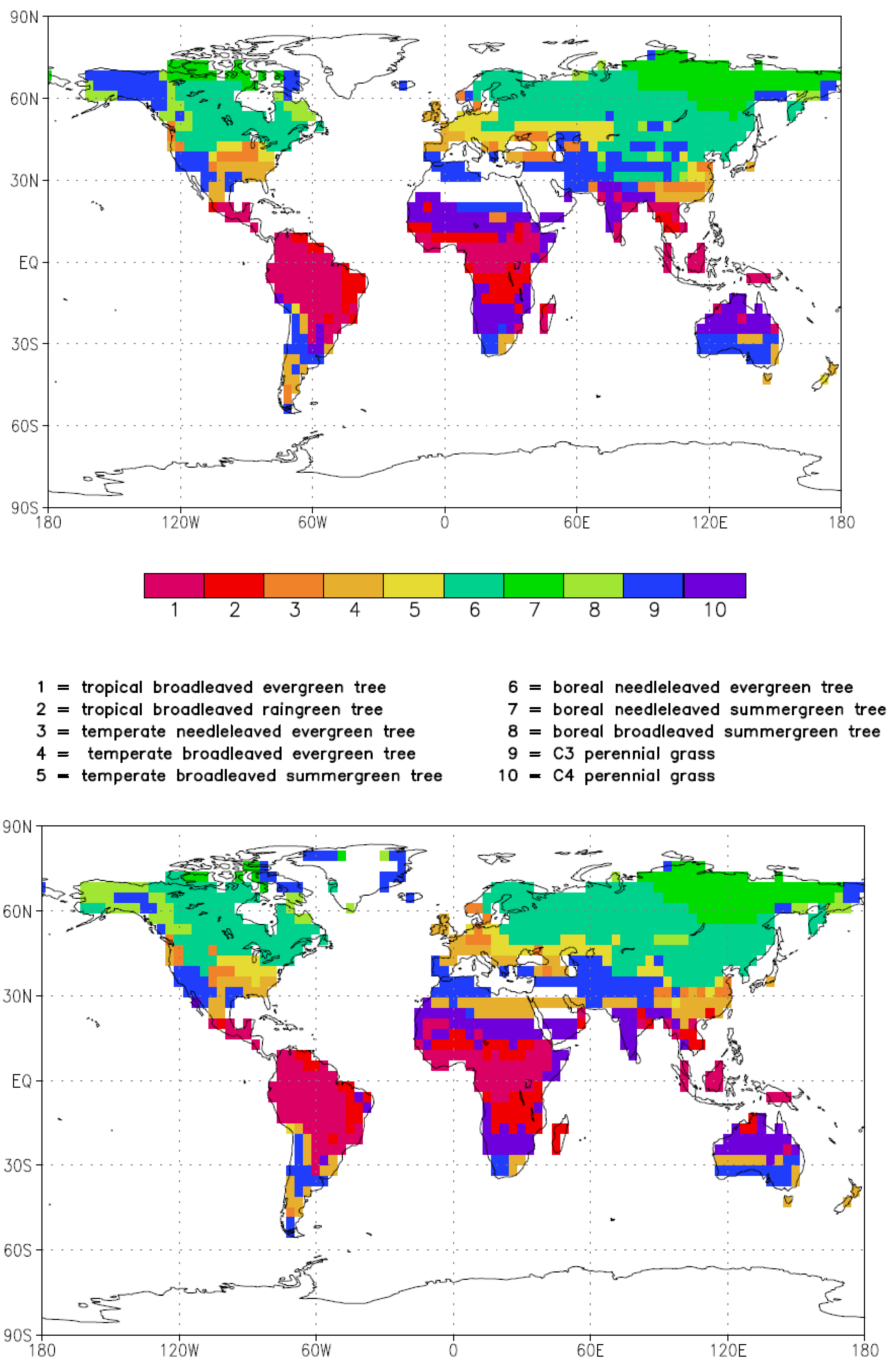
| vegetation | modern | modern | Micheels et al., (2007), [36] |
| Ocean: LSG | |||
| ocean gateways | modern | CAS 500 m | CAS 500 m |
| wind and hydrological cycle | from CTRL | from TGEO | from TVEG |
| salinity and temperature | calculated | calculated | calculated |
| Vegetation: LPJ | |||
| vegetation | calculated | - | calculated |
2.2. Dynamical Vegetation Model
2.3. Ocean Circulation Model
3. Results
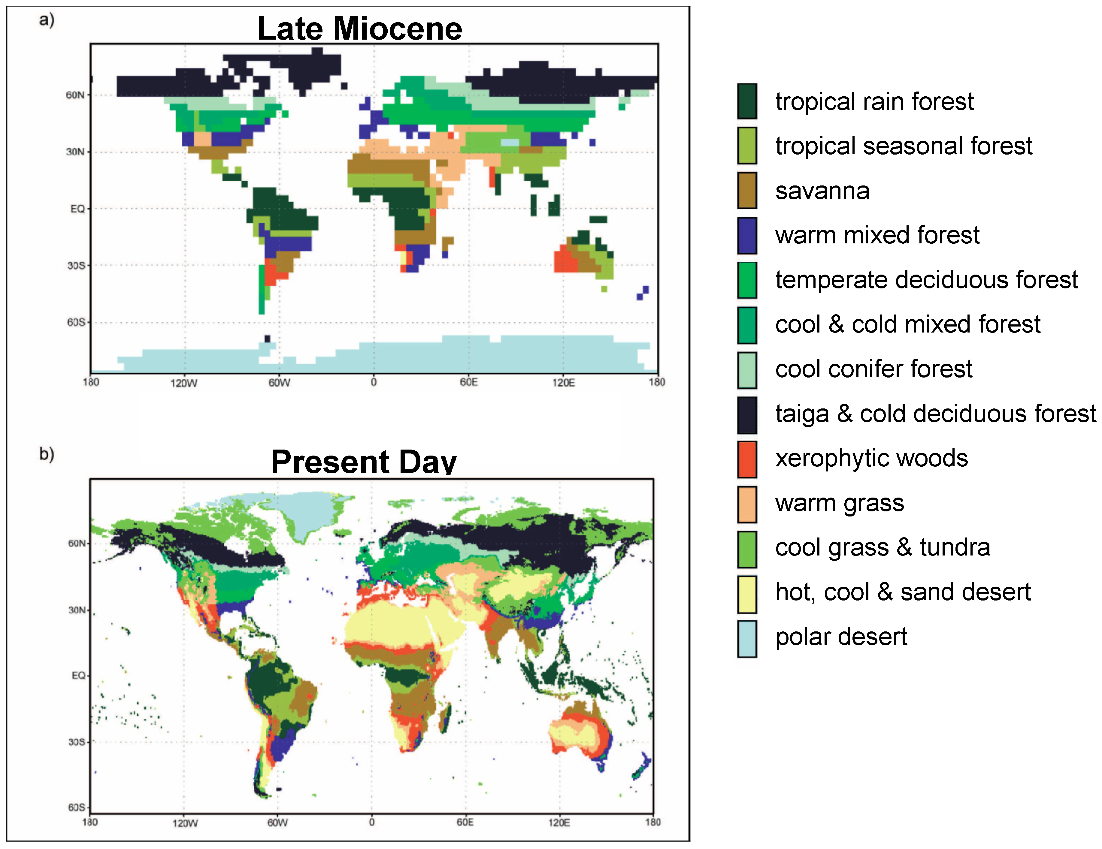
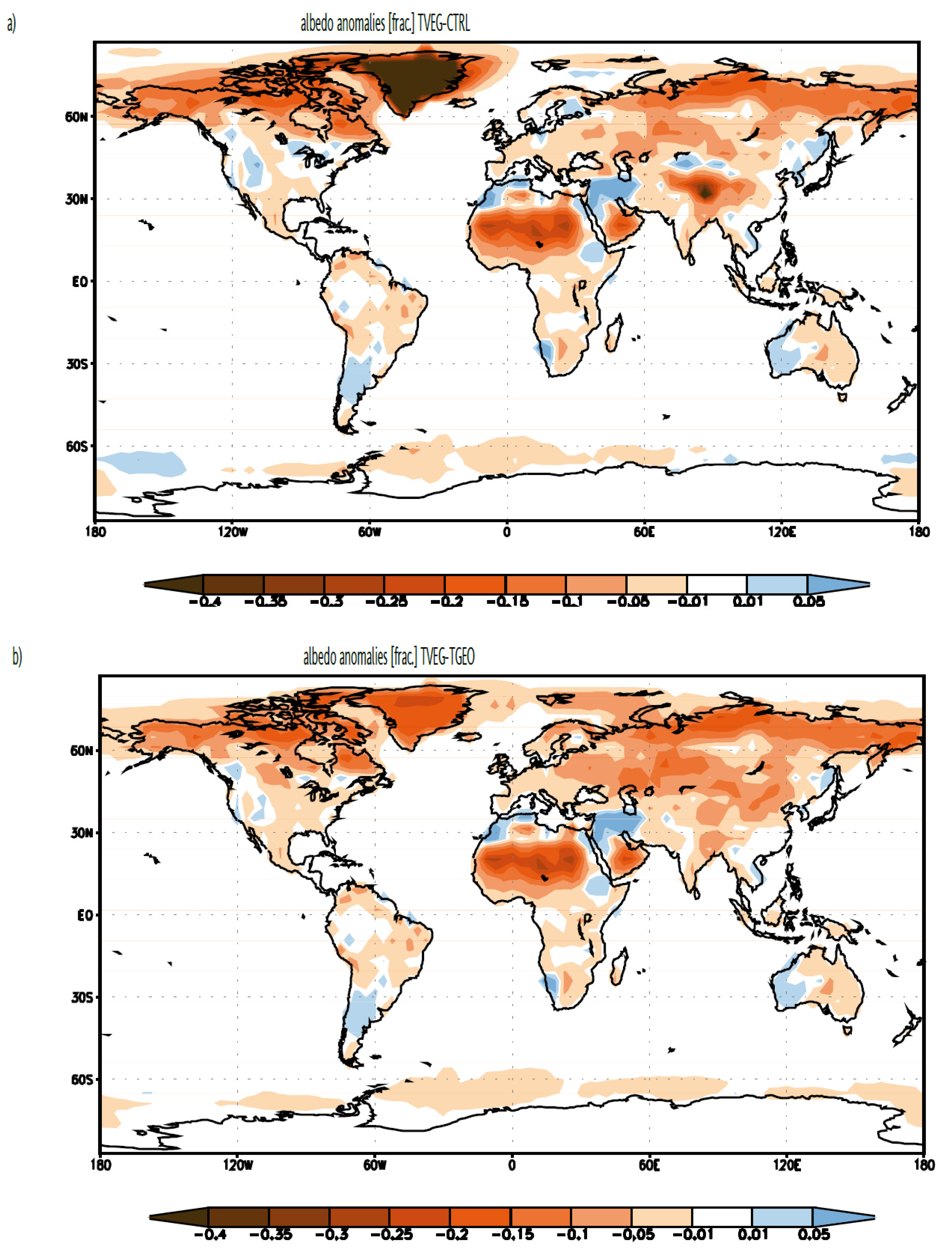
3.1. Albedo, Hydrological Cycle and Vegetation Cover


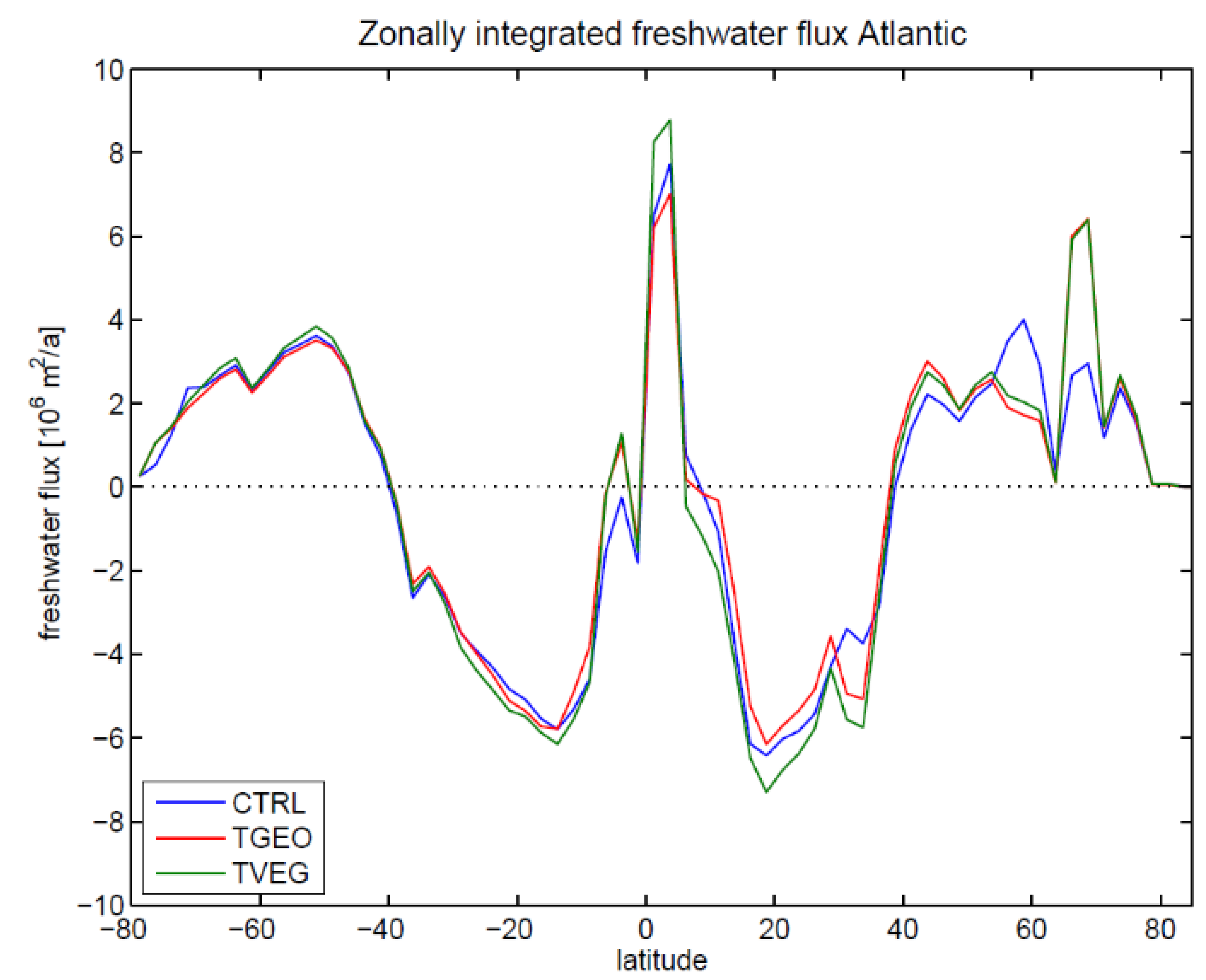


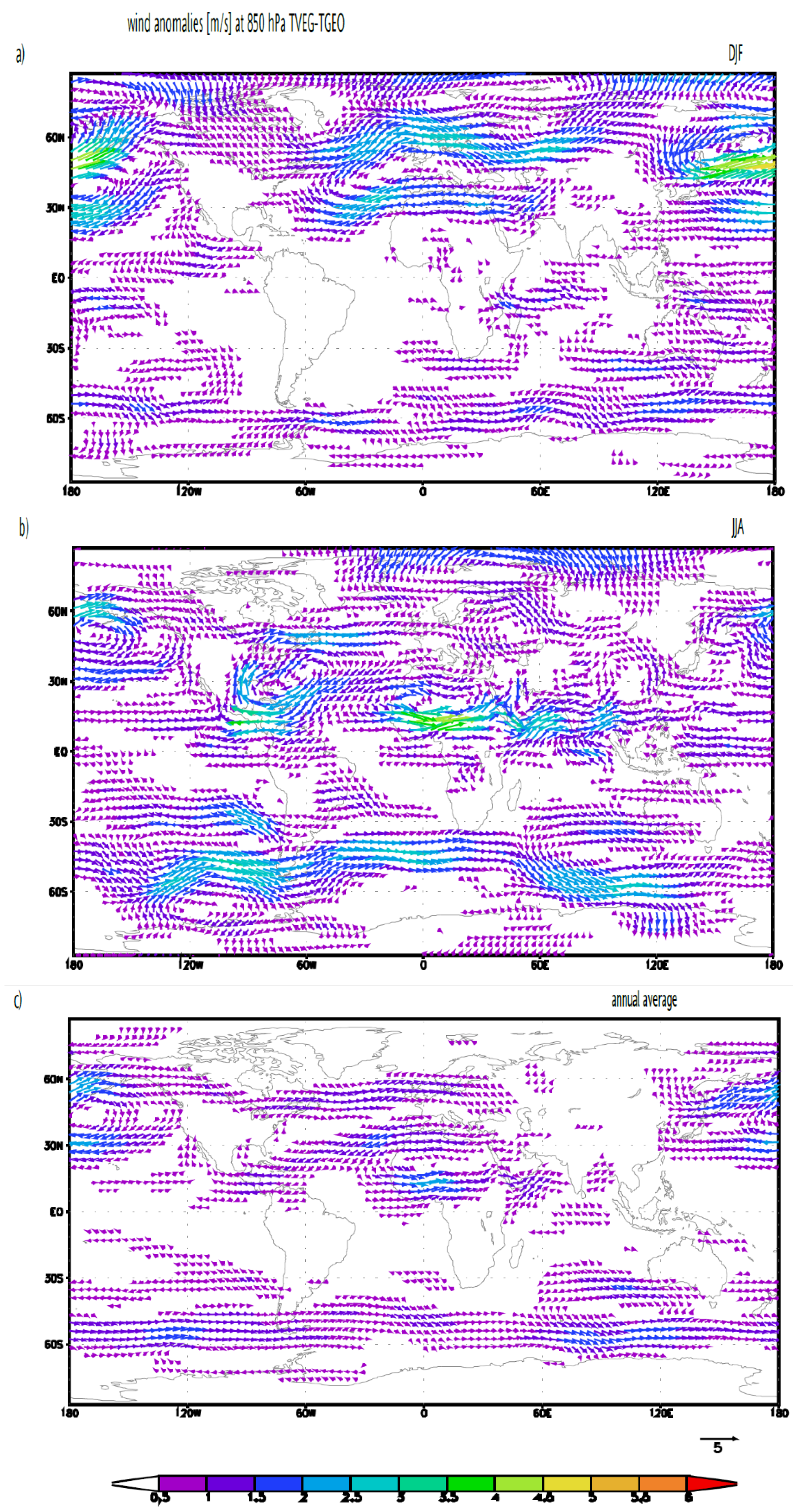
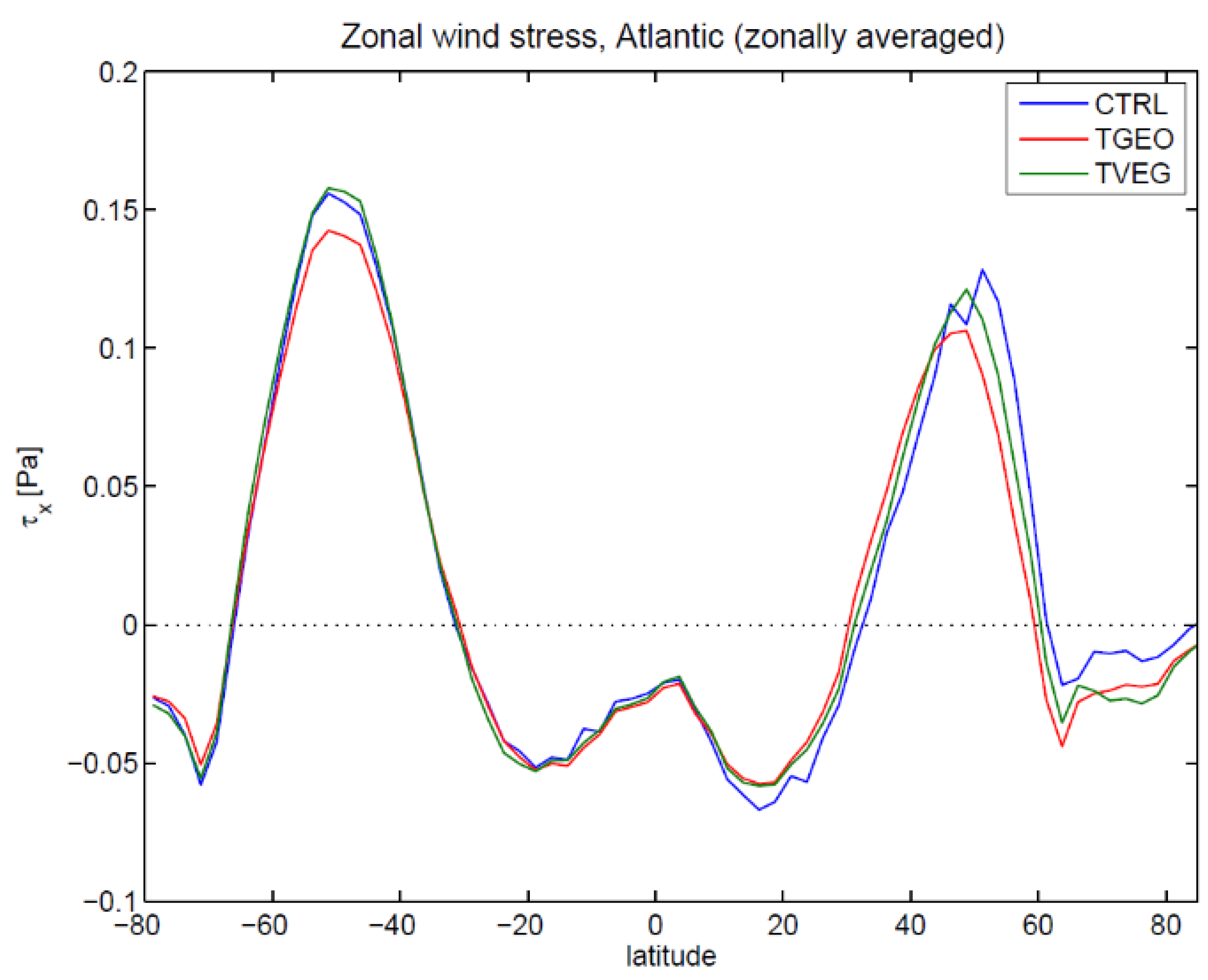
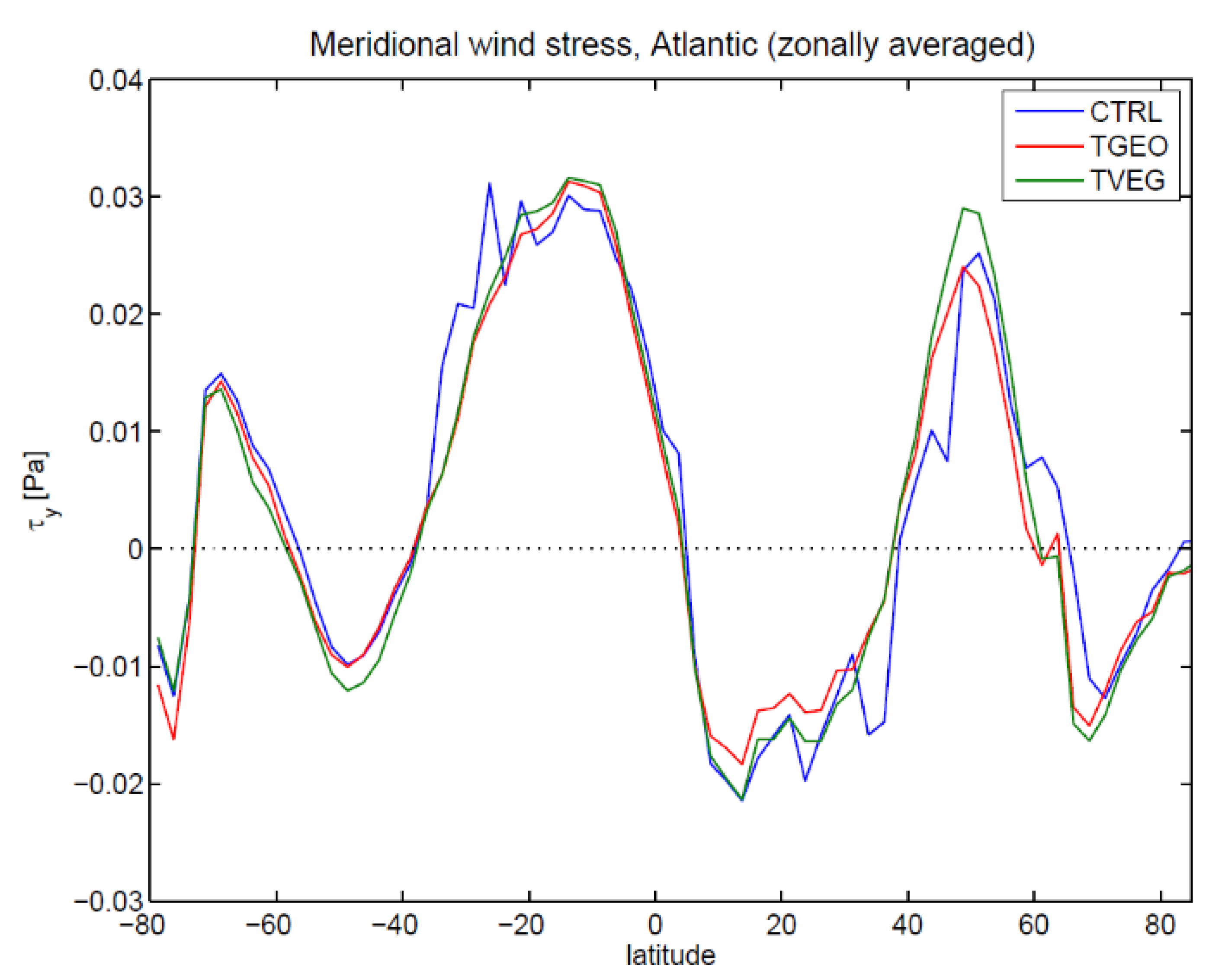
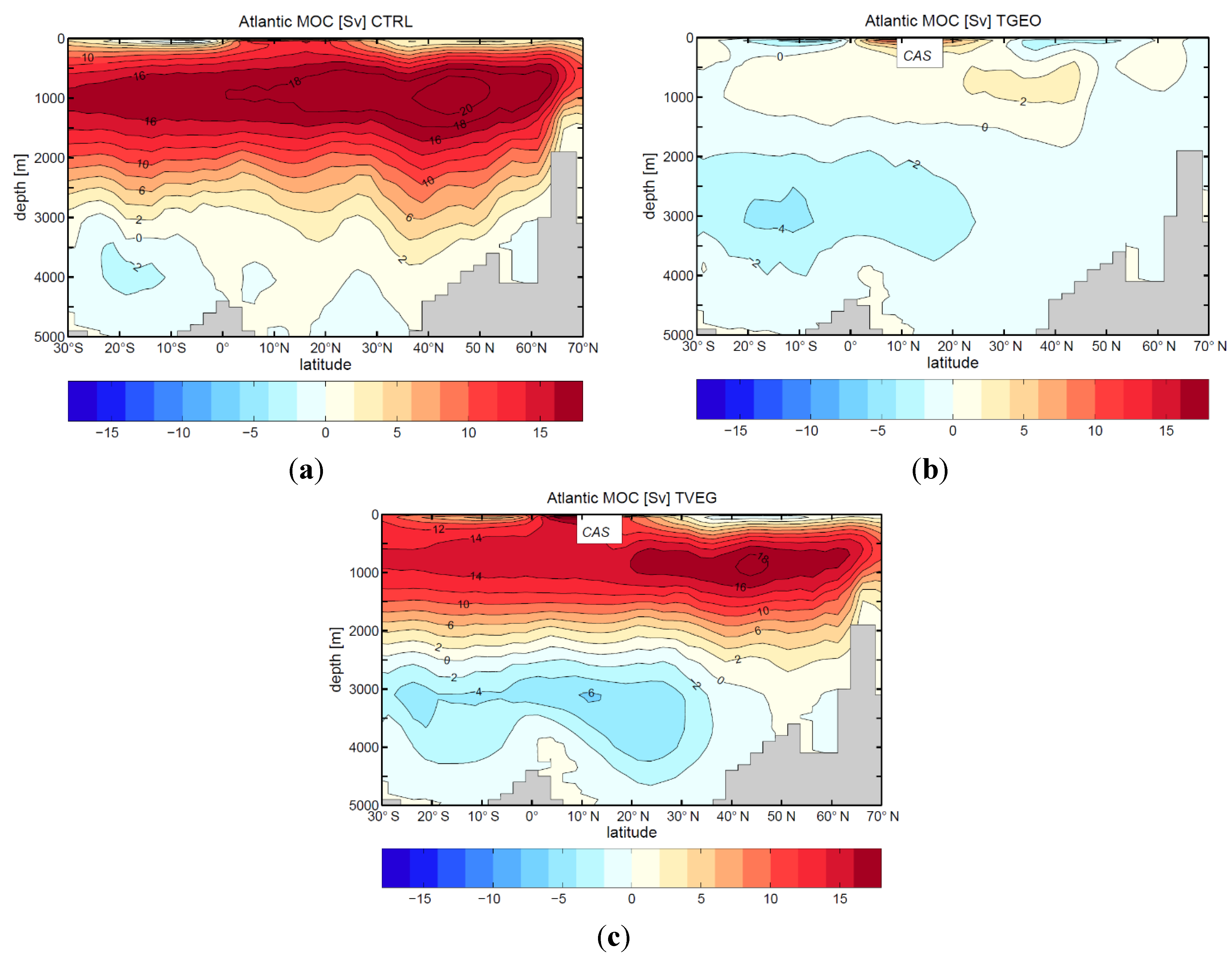
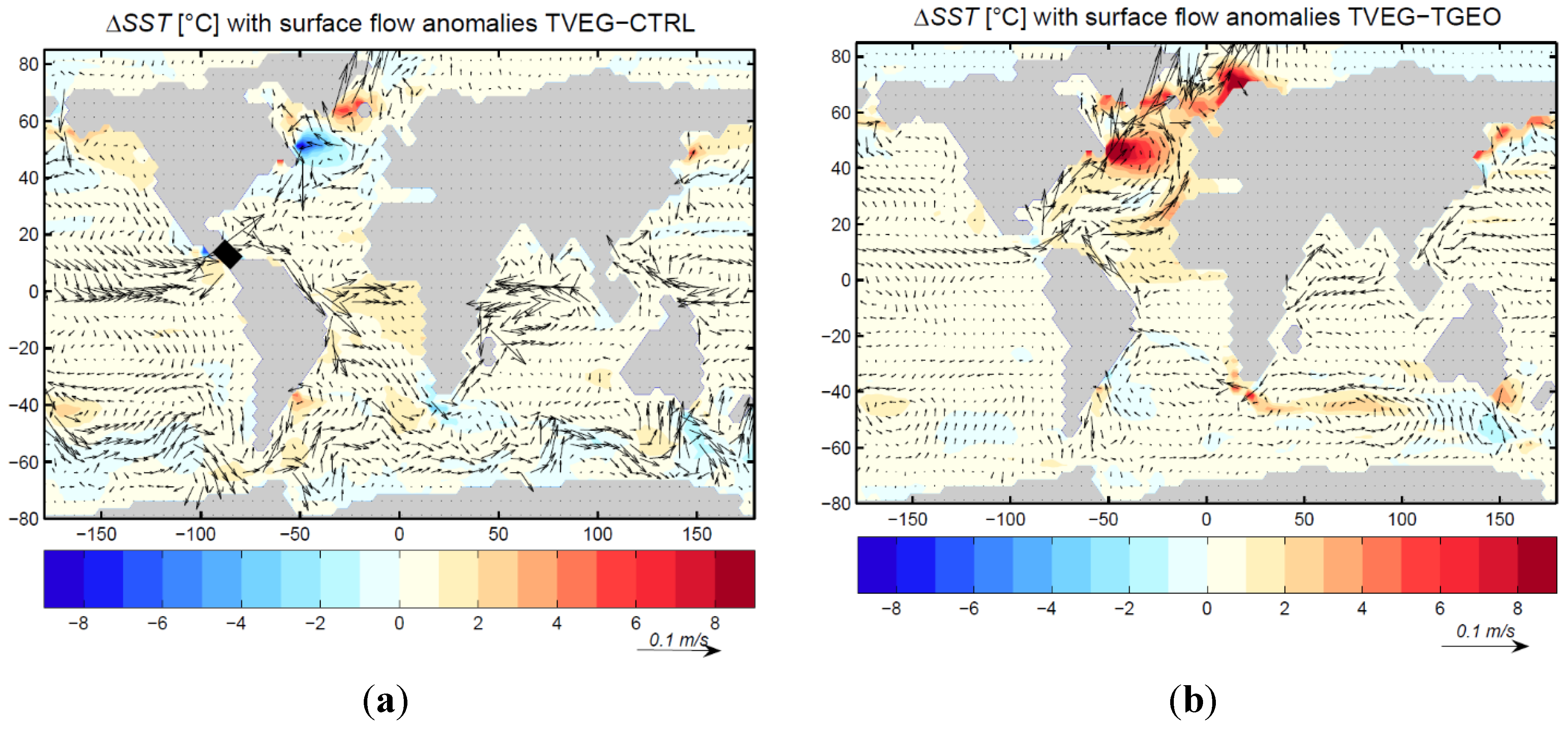
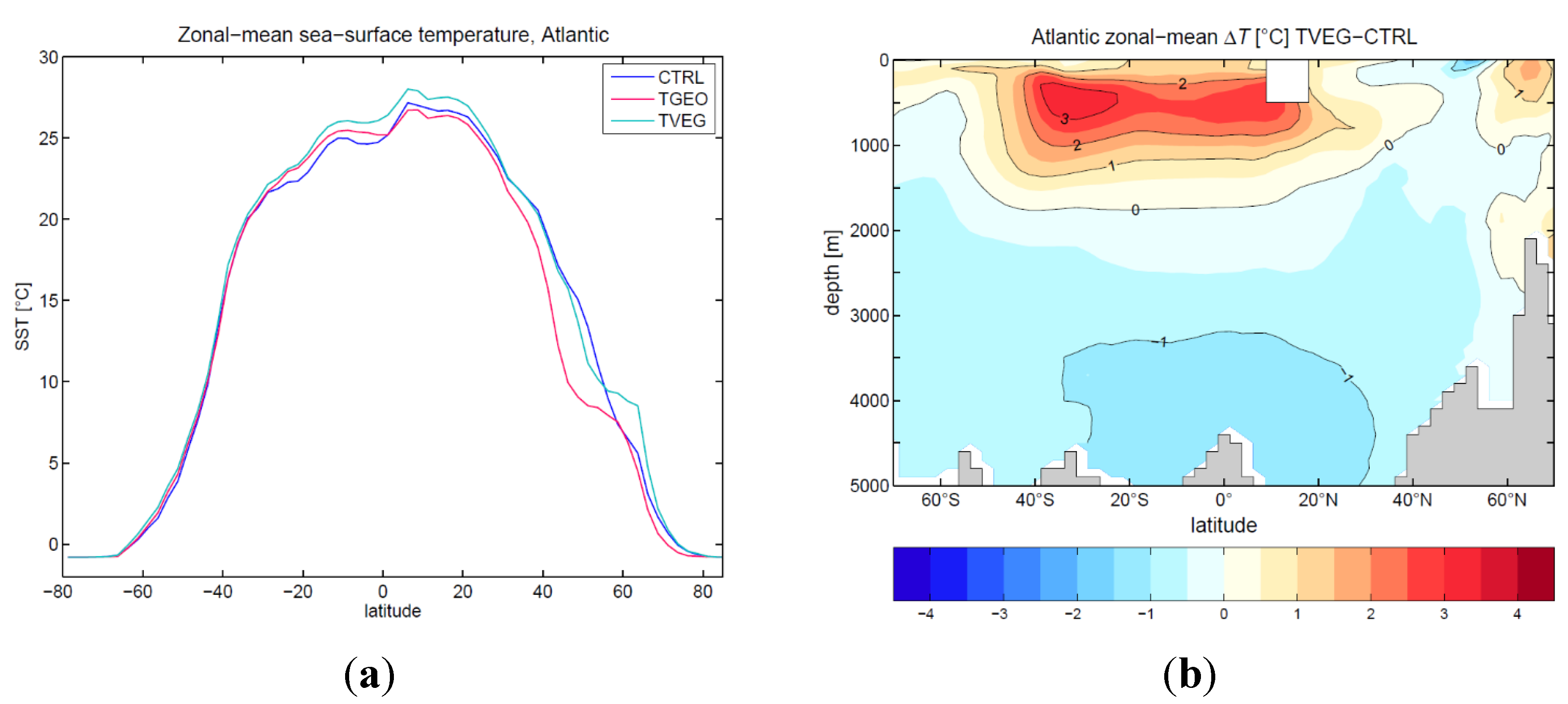
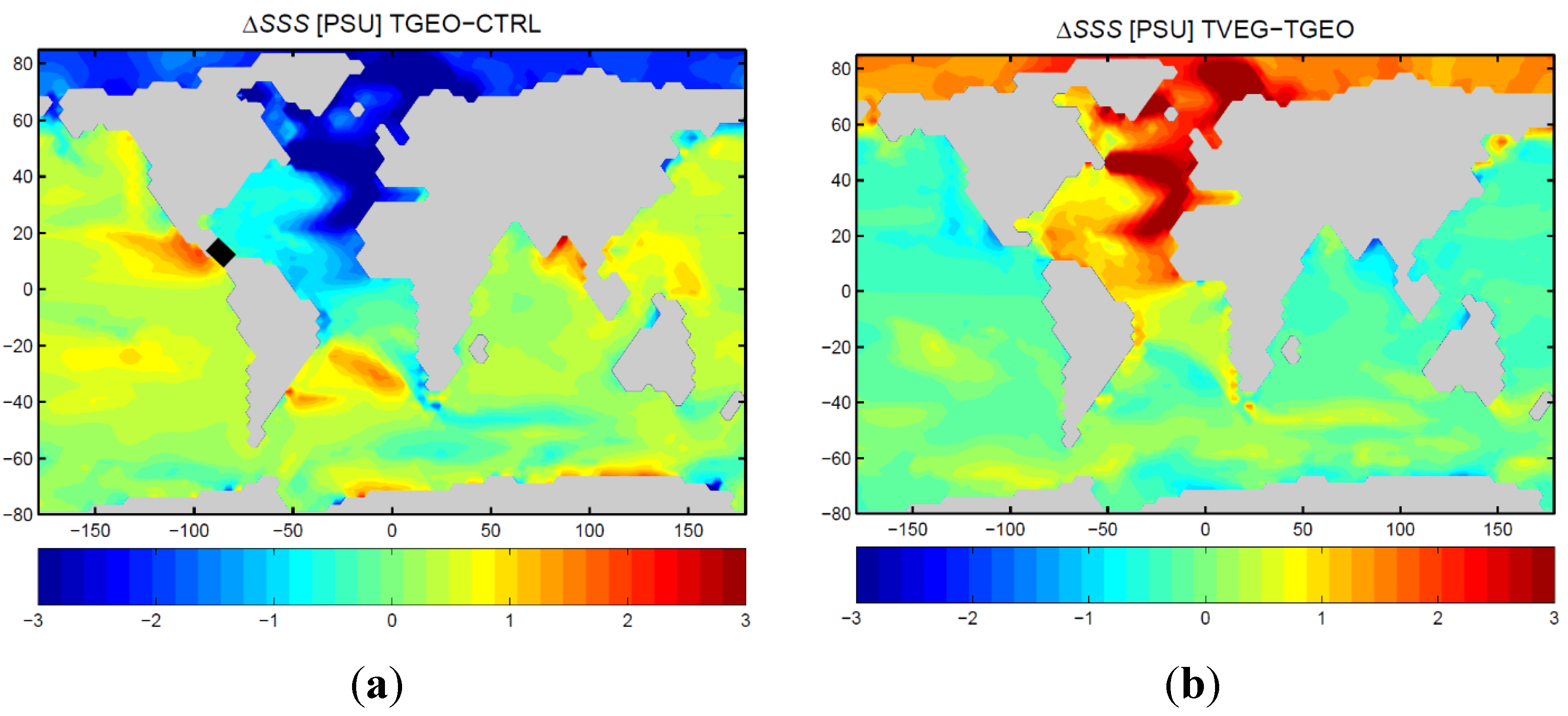
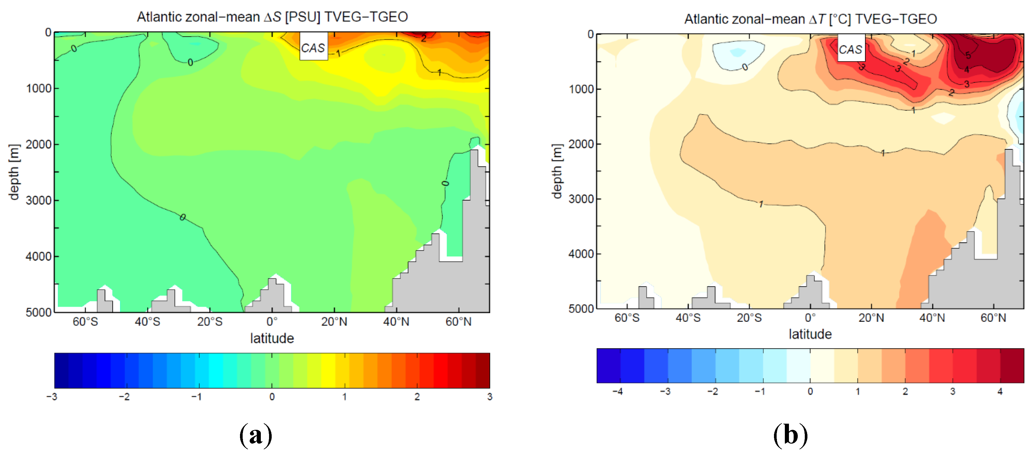
3.2. Ocean Circulation


4. Discussion
5. Conclusions
Acknowledgments
Author Contributions
Conflicts of Interest
References
- Zachos, J.; Pagani, M.; Sloan, L.; Thomas, E.; Billups, K. Trends, rhythms, and aberations in global climate 65 Ma to Present. Science 2001, 29, 686–693. [Google Scholar] [CrossRef] [PubMed]
- DeConto, R.M.; Pollard, D. Rapid Cenozoic glaciation of Antarctica induced by declining atmospheric CO2. Nature 2003, 421, 245–249. [Google Scholar] [CrossRef] [PubMed]
- Kennett, J.P. Cenozoic evolution of Antarctic glaciation, the Circum Antarctic Ocean, and their impact on global paleoceanography. J. Geophys. Res. 1977, 82, 3843–3860. [Google Scholar] [CrossRef]
- Wright, J.D.; Miller, K.G. Control of North Atlantic Deep Water circulation by the Greenland-Scotland Ridge. Paleoceanography 1996, 11, 157–169. [Google Scholar] [CrossRef]
- Billups, K. Late Miocene through early Pliocene deep water circulation and climate change viewed from the sub-Antarctic South Atlantic. Palaeogeogr. Palaeoclimatol. Palaeoecol. 2002, 185, 287–307. [Google Scholar] [CrossRef]
- Cane, M.A.; Molnar, P. Closing of the Indonesian seaway as a precursor to east African aridification around 3–4 million years ago. Nature 2001, 411, 157–161. [Google Scholar] [CrossRef] [PubMed]
- Lawver, L.A.; Gahagan, L.M. Evolution of Cenozoic seaways in the circum-Antarctic region. Palaeogeogr. Palaeoclimatol. Palaeoecol. 2003, 198, 11–37. [Google Scholar] [CrossRef]
- Flower, B.P.; Kennett, J.P. The middle Miocene climatic transition: East Antarctic ice sheet development, deep ocean circulation and global carbon cycling. Palaeogeogr. Palaeoclimatol. Palaeoecol. 1994, 108, 537–555. [Google Scholar] [CrossRef]
- Haug, G.; Tiedemann, R. Effect of the formation of the Isthmus of Panama on Atlantic Ocean thermohaline circulation. Nature 1998, 393, 673–676. [Google Scholar] [CrossRef]
- Mudelsee, M.; Bickert, T.; Lear, C.H.; Lohmann, G. Cenozoic climate changes: A review based on time series analysis of marine benthic δ18O records. Rev. Geophys. 2014, 52, 1–42. [Google Scholar] [CrossRef]
- Greenwood, D.R.; Wing, S.L. Eocene continental climates and latitudinal temperature gradients. Geology 1995, 23, 1044–1048. [Google Scholar] [CrossRef]
- Crowley, T.J.; Zachos, J.C. Comparison of zonal temperature profiles for past warm periods. In Warm Climates in Earth History; Huber, B., MacLeod, K.G., Wing, S.C., Eds.; Cambridge University Press: New York, NY, USA, 2000; pp. 50–76. [Google Scholar]
- Pound, M.; Haywood, A.M.; Salzman, U.; Riding, J.B. Global vegetation dynamics and latitudinal temperature gradients during the Mid to LateMiocene (15.97–5.33 Ma). Earth Sci. Rev. 2012, 112, 1–22. [Google Scholar] [CrossRef] [Green Version]
- Barron, E.J. Eocene equator-to-pole surface ocean temperature: A significant climate problem? Paleoceanography 1987, 2, 729–739. [Google Scholar] [CrossRef]
- Huber, M.; Sloan, L. Heat transport, deep waters and thermal gradients: Coupled climate simulation of an Eocene greenhouse climate. Geophys. Res. Lett. 2001, 28, 3481–3484. [Google Scholar] [CrossRef]
- Micheels, A.; Bruch, A.A.; Eronen, J.; Fortelius, M.; Harzhauser, M.; Utescher, T.; Mosbrugger, V. Analysis of heat transport mechanisms from a late Miocene model experiment with a fully-coupled atmosphere-ocean general circulation model. Palaeogeogr. Palaeoclimatol. Palaeoecol. 2011, 304, 337–350. [Google Scholar] [CrossRef]
- Schmidt, G.A.; Mysak, L.A. Can increased poleward oceanic heat flux explain the warm Cretaceous climate? Paleoceanography 1996, 11, 579–593. [Google Scholar] [CrossRef]
- Hay, W.W.; DeConto, R.M.; Wold, C.N. Climate: Is the past key to the future? Geol. Rundsch. 1997, 86, 471–491. [Google Scholar] [CrossRef]
- Caballero, R.; Langen, P. The dynamic range of poleward energy transport in an atmospheric general circulation model. Geophys. Res. Lett. 2005, 32. [Google Scholar] [CrossRef]
- Wright, J.D.; Miller, K.G.; Fairbanks, R.G. Miocene stable isotopes: Implications for deepwater circulation and climate. Paleoceanography 1992, 7, 357–389. [Google Scholar] [CrossRef]
- Montes, C.; Cardona, A.; Jaramillo, C.; Pardo, A.; Silva, J.C.; Valencia, V.; Pérez-Angel, L.C.; Ayala, C.; Rodriguez-Parra, L.A.; Ramirez, V.; et al. Middle Miocene closure of the Central American Seaway. Science 2015, 348, 226–229. [Google Scholar] [CrossRef] [PubMed]
- Mikolajewicz, U.; Maier-Reimer, E.; Crowley, T.J.; Kim, K.J. Effect of Drake and Panamanian gateways on the circulation of an ocean model. Paleoceanography 1993, 8, 409–426. [Google Scholar] [CrossRef]
- Bice, K.L.; Scotese, C.R.; Seidov, D.; Barron, E.J. Quantifying the role of geographic change in Cenozoic ocean heat transport using uncoupled atmosphere and ocean models. Palaeogeogr. Palaeoclimatol. Palaeoecol. 2000, 161, 295–310. [Google Scholar] [CrossRef]
- Retallack, G. Cenozoic expansion of grasslands and climatic cooling. J. Geol. 2001, 109, 407–426. [Google Scholar] [CrossRef]
- Willis, K.J.; McElwain, J.C. The Evolution of Plants; Oxford University Press: Oxford, UK, 2002; p. 378. [Google Scholar]
- Morley, R.J. Origin and Evolution of Tropical Rain Forests; Wiley: Chichester, UK, 2000; p. 362. [Google Scholar]
- Bredenkamp, G.J.; Spada, F.; Kazmieczak, E. On the origin of northern and southern hemisphere grasslands. Plant Ecol. 2002, 163, 209–229. [Google Scholar] [CrossRef]
- Cerling, T.E.; Harris, J.M.; MacFadden, B.J.; Leakey, M.G.; Quade, J.; Eisenmann, V.; Ehleringer, J.R. Global vegetation change through the Miocene/Pliocene boundary. Nature 1997, 389, 153–159. [Google Scholar] [CrossRef]
- Freeman, K.H.; Colarusso, L.A. Molecular and isotopic records of C4 grassland expansion in the late Miocene. Geochim. Cosmochim. Acta 2001, 65, 1439–1454. [Google Scholar] [CrossRef]
- Dutton, J.F.; Barron, E.J. Miocene to present vegetation changes: A possible piece of the Cenozoic puzzle. Geology 1997, 25, 39–41. [Google Scholar] [CrossRef]
- Otto-Bliesner, B.; Upchurch, G.R. Vegetation-induced warming of high-latitude regions during the Late Cretaceous period. Nature 1997, 385, 804–807. [Google Scholar] [CrossRef]
- Roeckner, E.; Arpe, K.; Bengtsson, L.; Christoph, M.; Claussen, M.; Dümenil, L.; Esch, M.; Giorgetta, M.; Schlese, U.; Schulzweida, U. The Atmospheric General Circulation Model ECHAM-4: Model Description and Simulation of Present-Day Climate, Max-Planck-Institut für Meteorologie; MPI Report No. 218; Max-Planck-Institute: Hamburg, Germany, 1996. [Google Scholar]
- Steppuhn, A.; Micheels, A.; Geiger, G.; Mosbrugger, V. Reconstructing the Late Miocene Climate and oceanic heat flux using the AGCM ECHAM4 coupled to a mixed-layer ocean model with adjusted flux correction. Palaeogeogr. Palaeoclimatol. Palaeoecol. 2006, 238, 399–423. [Google Scholar] [CrossRef]
- Freeman, H.H.; Hayes, J.M. Fractionation of carbon isotopes by phytoplankton and estimates of ancient CO2 levels. Global Biogeochem. Cycles 1992, 6, 185–198. [Google Scholar] [CrossRef] [PubMed]
- Pagani, M.; Arthur, M.A.; Freeman, K.H. Miocene evolution of atmospheric carbon dioxide. Paleoceanography 1999, 14, 273–292. [Google Scholar] [CrossRef]
- Pearson, P.N.; Palmer, M.R. Atmospheric carbon dioxide concentrations over the past 600 million years. Nature 2000, 406, 695–699. [Google Scholar] [CrossRef] [PubMed]
- Demicco, R.V.; Lowenstein, T.K.; Hardie, L.A. Atmospheric pCO2 since 60 Ma from records of seawater pH, calcium and primary carbonate mineralogy. Geology 2003, 31, 793–796. [Google Scholar] [CrossRef]
- Pagani, M.; Zachos, J.C.; Freeman, K.H.; Tipple, B.; Bohaty, S. Marked decline in atmospheric carbon dioxide concentrations during the Paleogene. Science 2005, 309, 600–603. [Google Scholar] [CrossRef] [PubMed]
- Kürschner, W.M.; Kvaček, Z.; Dilcher, D.L. The impact of Miocene atmospheric carbon dioxide fluctuations on climate and the evolution of terrestrial ecosystems. PNAS 2008, 105, 449–453. [Google Scholar] [CrossRef] [PubMed]
- Zhang, Y.G.; Pagani, M.; Liu, Z.; Bohaty, S.M.; Deconto, R. A 40-million-year history of atmospheric CO2. Philos. Trans. A Math. Phys. Eng. Sci. 2013, 371. [Google Scholar] [CrossRef] [PubMed]
- Knorr, G.; Butzin, M.; Micheels, A.; Lohmann, G. A Warm Miocene Climate at Low Atmospheric CO2 levels. Geophys. Res. Lett. 2011. [Google Scholar] [CrossRef]
- New, M.; Hulme, M.; Jones, P. Representing Twentieth-Century Space–Time Climate Variability. Part I: Development of a 1961–90 Mean Monthly Terrestrial Climatology. J. Climate 1999, 12, 829–856. [Google Scholar] [CrossRef]
- Micheels, A. Late Miocene climate modelling with ECHAM4/ML—The effects of the palaeovegetation on the Tortonian climate. Ph.D. Thesis, University of Tübingen, Tübingen, Germany, 2003; p. 110. [Google Scholar]
- Micheels, A.; Bruch, A.A.; Uhl, D.; Utescher, T.; Mosbrugger, V. A Late Miocene climate model simulation with ECHAM4/ML and its quantitative validation with terrestrial proxy data. Palaeogeogr. Palaeoclimatol. Palaeoecol. 2007, 253, 251–270. [Google Scholar] [CrossRef]
- Pickford, M. Crocodiles from the Beglia Formation, Middle/Late Miocene Boundary, Tunisia, and their significance for Saharan palaeoclimatology. Ann. Paleontol. 2000, 86, 59–67. [Google Scholar] [CrossRef]
- Micheels, A.; Eronen, J.; Mosbrugger, V. The Late Miocene climate response to a modern Sahara desert. Global Planet. Chang. 2009, 67, 193–204. [Google Scholar] [CrossRef]
- Vignaud, P.; Duringer, P.; Mackaye, H.T.; Likius, A.; Blondel, C.; Boisserie, J.-R.; de Bonis, L.; Eisenmann, V.; Etienne, M.E.; Geraads, D.; et al. Geology and paleontology of the Upper Miocene Toros-Menalla hominidlocality, Chad. Nature 2002, 418, 152–155. [Google Scholar] [CrossRef] [PubMed]
- Wolfe, J.A. Distribution of major vegetational types during the Tertiary. In The Carbon Cycle and Atmospheric CO2 Natural Variations Archean to Present; Sundquist, E.T., Broecker, W.S., Eds.; American Geophysical Union: Washington, DC, USA, 1985; pp. 357–375. [Google Scholar]
- Sitch, S.; Smith, B.; Prentice, I.C.; Arneth, A.; Bondeau, A.; Cramer, W.; Kaplan, J.O.; Levis, S.; Lucht, W.; Sykes, M.T.; et al. Evaluation of ecosystem dynamics, plant geography and terrestrial carbon cycling in the LPJ dynamic global vegetation model. Global Chang. Biol. 2003, 9, 161–185. [Google Scholar] [CrossRef]
- Kaplan, J.O.; Prentice, I.C.; Knorr, W.; Valdes, P.J. Modelling the dynamics of terrestrial carbon storage since the Last Glacial Maximum. Geophys. Res. Lett. 2002, 29, 2074–2078. [Google Scholar] [CrossRef]
- Scholze, M.; Knorr, W.; Heimann, M. Modelling terrestrial vegetation dynamics and carbon cycling for an abrupt climate change event. Holocene 2003, 13, 327–333. [Google Scholar] [CrossRef]
- Maier-Reimer, E.; Mikolajewicz, U.; Hasselmann, K. Mean circulation of the Hamburg LSG OGCM and its sensitivity to the thermohaline surface forcing. J. Phys. Oceanogr. 1993, 23, 731–757. [Google Scholar] [CrossRef]
- Schäfer-Neth, C.; Paul, A. Circulation of the glacial Atlantic: A synthesis of global and regional modeling. In The northern North Atlantic: A changing environment; Schäfer, P., Ritzrau, W., Schlüter, M., Thiede, J., Eds.; Springer: Berlin, Germany, 2001; pp. 446–462. [Google Scholar]
- Prange, M.; Romanova, V.; Lohmann, G. The glacial thermohaline circulation: Stable or unstable? Geophys. Res. Lett. 2002, 29. [Google Scholar] [CrossRef] [Green Version]
- Prange, M.; Lohmann, G.; Paul, A. Influence of vertical mixing on the thermohaline hysteresis: Analyses of an OGCM. J. Phys. Oceanogr. 2003, 33, 1707–1721. [Google Scholar] [CrossRef]
- Lohmann, G. The influence of a near-bottom transport parameterization on the sensitivity of the thermohaline circulation. J. Phys. Oceanogr. 1998, 28, 2095–2103. [Google Scholar] [CrossRef]
- Lohmann, G.; Schulz, M. Reconciling Bølling warmth with peak deglacial meltwater discharge. Paleoceanography 2000, 15, 537–540. [Google Scholar] [CrossRef]
- Butzin, M.; Prange, M.; Lohmann, G. Radiocarbon simulations for the glacial ocean: The effects of wind stress, Southern Ocean sea ice and Heinrich events. Earth Planet. Sci. Lett. 2005, 235, 45–61. [Google Scholar] [CrossRef]
- Lohmann, G.; Gerdes, R. Sea ice effects on the sensitivity of the thermohaline circulation in simplified atmosphere-ocean-sea ice models. J. Clim. 1998, 11, 2789–2803. [Google Scholar] [CrossRef]
- Knorr, G.; Lohmann, G. Southern Ocean origin for resumption of Atlantic thermohaline circulation during deglaciation. Nature 2003, 424, 532–536. [Google Scholar] [CrossRef] [PubMed]
- Boulter, M.C.; Manum, S.B. A lost continent in temperate Arctic. Endevour 1997, 21, 105–108. [Google Scholar] [CrossRef]
- Schuster, M.; Duringer, P.; Ghienne, J.-F.; Vignaud, P.; Mackaye, H.T.; Likius, A.; Brunet, M. The Age of the Sahara Desert. Science 2006, 311. [Google Scholar] [CrossRef] [PubMed]
- Lohmann, G. Atmospheric and oceanic freshwater transport during weak Atlantic overturning circulation. Tellus A 2003, 55, 438–449. [Google Scholar] [CrossRef]
- Schmitz, W.J. On the interbasin scale thermohaline circulation. Rev. Geophys. 1995, 33, 151–173. [Google Scholar] [CrossRef]
- Macdonald, A.M.; Wunsch, C. An estimate of global ocean circulation and heat fluxes. Nature 1996, 382, 436–439. [Google Scholar] [CrossRef]
- Wolfe, J.A. An analysis of Neogene climates in Beringia. Palaeogeogr. Palaeoclimatol. Palaeoecol. 1994, 108, 207–216. [Google Scholar] [CrossRef]
- Bradshaw, C.D.; Lunt, D.J.; Flecker, R.; Davies-Barnard, T. Disentangling the roles of late Miocene palaeogeography and vegetation—Implications for climate sensitivity. Palaeogeogr. Palaeoclimatol. Palaeoecol. 2015, 417, 17–34. [Google Scholar] [CrossRef]
- Herold, N.; Huber, M.; Müller, R.D.; Seton, M. Modeling the Miocene climatic optimum: Ocean circulation. Paleoceanography 2012, 27. [Google Scholar] [CrossRef]
- Wolf, T.C.W.; Thiede, J. History of terrigenous sedimentation during the past 10 m.y. in the North Atlantic (ODP Legs 104 and 105 and DSDP Leg 81). Mar. Geol. 1991, 101, 83–102. [Google Scholar] [CrossRef]
- Lohmann, G.; Lorenz, S. On the hydrological cycle under paleoclimatic conditions as derived from AGCM simulations. J. Geophys. Res. 2000, 105, 417–436. [Google Scholar] [CrossRef]
- Broecker, W.S. The salinity contrast between the Atlantic and Pacific during glacial time. Paleoceanography 1992, 4, 207–212. [Google Scholar] [CrossRef]
- Zaucker, F.; Broecker, W.S. The influence of atmospheric moisture transport on fresh water balance of the Atlantic drainage basin: General circulation model simulations and observations. J. Geophys. Res. 1992, 97, 2765–2773. [Google Scholar] [CrossRef]
- Zaucker, F.; Stocker, T.F.; Broecker, W.S. Atmospheric freshwater fluxes and their effect on the global thermohaline circulation. J. Geophys. Res. 1994, 99, 12443–12457. [Google Scholar] [CrossRef]
- Schmittner, A.; Appenzeller, C.; Stocker, T.F. Enhanced Atlantic freshwater export during El Niño. Geophys. Res. Lett. 2000, 27, 1163–1166. [Google Scholar] [CrossRef]
- Soden, B.J. The sensitivity of the tropical hydrological cycle to ENSO. J. Clim. 2000, 13, 538–549. [Google Scholar] [CrossRef]
- Latif, M.; Roeckner, E.; Mikolajewicz, U.; Voss, R. Tropical stabilization of the thermohaline circulation in a greenhouse warming simulation. J. Clim. 2000, 13, 1809–1813. [Google Scholar] [CrossRef]
- Fedorov, V.; Dekens, P.S.; McCarthy, M.; Ravelo, A.C.; deMenocal, P.B.; Barreiro, M.; Pacanowski, R.C.; Philander, S.G. The Pliocene paradox (Mechanisms for a permanent El Niño). Science 2006, 312, 1485–1489. [Google Scholar] [CrossRef] [PubMed]
- LaRiviere, J.P.; Ravelo, A.C.; Crimmins, A.; Dekens, P.S.; Ford, H.L.; Lyle, M.; Wara, M.W. Late Miocene decoupling of oceanic warmth and atmospheric carbon dioxide forcing. Nature 2012, 486, 97–100. [Google Scholar] [CrossRef] [PubMed]
- Goldner, A.; Herold, N.; Huber, M. The challenge of simulating the warmth of the mid-Miocene climatic optimum in CESM1. Clim. Past 2014, 10, 523–536. [Google Scholar] [CrossRef]
- Sloan, L.C.; Pollard, D. Polar stratospheric clouds: A high latitude warming mechanism in an ancient greenhouse world. Geophys. Res. Lett. 1998, 25, 3517–3520. [Google Scholar] [CrossRef]
- Emanuel, K. A simple model for multiple climate regimes. J. Geophys. Res. 2002, 107. [Google Scholar] [CrossRef]
- Lear, C.H.; Rosenthal, Y.; Wright, J.D. The closing of a seaway: Ocean water masses and global climate change. Earth Planet. Sci. Lett. 2003, 210, 425–436. [Google Scholar] [CrossRef]
- Billups, K.; Channell, J.E.T.; Zachos, J. Late Oligocene to early Miocene geochronology and paleoceanography. Paleoceanography 2002, 17. [Google Scholar] [CrossRef]
- Sluijs, A.; Schouten, S.; Pagani, M.; Woltering, M.; Brinkhuis, H.; Sinninghe Damste, J.S.; Dickens, G.R.; Huber, M.; Reichart, G.-J.; Stein, R.; et al. Subtropical Arctic Ocean temperatures during the Palaeocene/Eocene thermal maximum. Science 2006, 441, 610–613. [Google Scholar] [CrossRef]
- Lohmann, G.; Pfeiffer, M.; Laepple, T.; Leduc, G.; Kim, J.-H. A model-data comparison of the Holocene global sea surface temperature evolution. Clim. Past 2013, 9, 1807–1839. [Google Scholar] [CrossRef] [Green Version]
- Bradshaw, C.D.; Lunt, D.J.; Flecker, R.; Salzmann, U.; Pound, M.J.; Haywood, A.M.; Eronen, J.T. The relative roles of CO2 and palaeogeography in determining late Miocene climate: Results from a terrestrial model-data comparison. Clim. Past 2012, 8, 1257–1285. [Google Scholar] [CrossRef]
- Frank, M.; O’Nions, R.K.; Hein, J.R.; Banakar, V.K. 60 Ma records of major elements and Pb-Nd isotopes from hydrogenous ferromanganese crusts: Reconstruction of seawater paleochemistry. Geochim. Cosmochim. Acta 1999, 63, 1689–1708. [Google Scholar] [CrossRef]
- Frank, M.; Whiteley, N.; Kasten, S.; Hein, J.R.; O’Nions, R.K. North Atlantic Deep Water export to the Southern Ocean over the past 14 Myr: Evidence from Nd and Pb isotopes in ferromanganese crusts. Paleoceanography 2002, 17. [Google Scholar] [CrossRef]
- Delaney, M.; Boyle, E.A. Cd/Ca in Late Miocene benthic foraminifera and changes in the global organic carbon budget. Nature 1987, 330, 156–159. [Google Scholar] [CrossRef]
- Butzin, M.; Lohmann, G.; Bickert, T. Miocene ocean circulation inferred from marine carbon cycle modeling combined with benthic isotope records. Paleoceanography 2011, 26. [Google Scholar] [CrossRef]
- Zhang, Z.-S.; Nisancioglu, K.H.; Chandler, M.A.; Haywood, A.M.; Otto-Bliesner, B.L.; Ramstein, G.; Stepanek, C.; Abe-Ouchi, A.; Chan, W.-L.; Bragg, F.J.; et al. Mid-Pliocene Atlantic Meridional Overturning Circulation not unlike modern? Clim. Past 2013, 9, 1495–1504. [Google Scholar] [CrossRef]
- Stepanek, C.; Lohmann, G. Modelling mid-Pliocene climate with COSMOS. Geosci. Model Dev. 2012, 5, 1221–1243. [Google Scholar] [CrossRef] [Green Version]
- Lyle, M.; Barron, J.; Bralower, J.; Huber, M.; Lyle, A.O.; Ravelo, A.C.; Rea, R.K.; Wilson, P. Pacific Ocean and cenozoic evolution of climate. Rev. Geophys. 2008, 46. [Google Scholar] [CrossRef]
- Knorr, G.; Lohmann, G. A warming climate during the Antarctic ice sheet growth at the Middle Miocene transition. Nat. Geosci. 2014, 7, 376–381. [Google Scholar] [CrossRef]
© 2015 by the authors; licensee MDPI, Basel, Switzerland. This article is an open access article distributed under the terms and conditions of the Creative Commons Attribution license ( http://creativecommons.org/licenses/by/4.0/).
Share and Cite
Lohmann, G.; Butzin, M.; Bickert, T. Effect of Vegetation on the Late Miocene Ocean Circulation. J. Mar. Sci. Eng. 2015, 3, 1311-1333. https://doi.org/10.3390/jmse3041311
Lohmann G, Butzin M, Bickert T. Effect of Vegetation on the Late Miocene Ocean Circulation. Journal of Marine Science and Engineering. 2015; 3(4):1311-1333. https://doi.org/10.3390/jmse3041311
Chicago/Turabian StyleLohmann, Gerrit, Martin Butzin, and Torsten Bickert. 2015. "Effect of Vegetation on the Late Miocene Ocean Circulation" Journal of Marine Science and Engineering 3, no. 4: 1311-1333. https://doi.org/10.3390/jmse3041311