Wind Turbine Blade Life-Time Assessment Model for Preventive Planning of Operation and Maintenance

Abstract

Out of the total wind turbine failure events, blade damage accounts for a substantial part, with some studies estimating it at around 23%. Current operation and maintenance (O&M) practices typically make use of corrective type maintenance as the basic approach, implying high costs for repair and replacement activities as well as large revenue losses, mainly in the case of offshore wind farms. The recent development and evolution of condition monitoring techniques, as well as the fact that an increasing number of installed turbines are equipped with online monitoring systems, offers a large amount of information on the blades structural health to the decision maker. Further, inspections of the blades are often performed in connection with service. In light of the obtained information, a preventive type of maintenance becomes feasible, with the potential of predicting the blades remaining life to support O&M decisions for avoiding major failure events. The present paper presents a fracture mechanics based model for estimating the remaining life of a wind turbine blade, focusing on the crack propagation in the blades adhesive joints. A generic crack propagation model is built in Matlab based on a Paris law approach. The model is used within a risk-based maintenance decision framework to optimize maintenance planning for the blades lifetime.

1. Introduction

Operation and maintenance (O&M) activities have been shown to contribute to around 25%–30% of the total energy cost from offshore wind power [1], leading to an increased effort for optimizing maintenance plans. This however is not a trivial task, due to the multitude of elements present in a turbine system, along with the limited understanding of their behavior, interactions and degradation and failure mechanisms. As a result, current practice within the industry is mainly based on a corrective maintenance approach, resulting in considerable costs from repairs and revenue losses.

At the same time, modern wind farms are installed with condition monitoring (CM) systems that offer a continuous influx of information on various behavioral and environmental parameters. Information from CM can potentially be used to assess the current health state of the turbine, thus offering large potential for preventive based maintenance planning.

This paper presents a lifetime analysis of an offshore wind turbine using a physical degradation model based on wind measurements for preventive maintenance, and focuses on analyzing the effect of different decision parameters on the total expected O&M cost.

For simplicity, the model is built for analyzing a single component, namely the rotor blade, as it was noted that this element has a relatively large failure frequency compared to other elements, covering around 25% of the total number of turbine breakdowns [2].

2. Optimal Maintenance and Inspection Planning

A framework for optimal inspection planning for wind turbines, using pre-posterior decision theory, was presented in [3] and serves as a basis for the maintenance model presented in this paper. Another application of this particular framework can be found in [4]. The optimization problem is briefly summarized in this section.

The maintenance decisions and different possible outcomes during the turbines life can be represented by a decision tree, as shown in Figure 1.

Figure 1. Decision tree for optimal operation and maintenance (O&M) planning.

Figure 1. Decision tree for optimal operation and maintenance (O&M) planning.

The vector z contains the initial design parameters of the component. These parameters model the physical behavior of the component and have a great influence on the damage model. Ideally, an optimization between fatigue life and initial cost is made in the design stage to reduce expected O&M costs.

The maintenance activities are represented in the outlined box. First, a decision is made with regards to the inspection/monitoring plan, represented by vector e. This decisions focuses on the time and type of inspection. It is important to note that a damage model is required in order to assess a probable outcome of the inspection. The outcome is modeled as a stochastic variable and its variance is dependent on the accuracy of the damage model and the reliability of the chosen inspection method. Once an outcome is generated, it is stored in S. Finally, a decision is made on what action should be taken for each of the possible inspection outcomes. These decision rules are noted d(S) and are mainly focused on whether or not an intervention should be made, based on the component’s health state.

The vector X accounts for the uncertainties present in the model and contains realizations of the stochastic variables, aiming at uncertainties governing wind/wave climate, strengths and degradation parameters, and also model uncertainties.

W represents the utility, expressed in monetary terms, resulting from each branch. The cost benefit B is expressed by the price of power generated during the turbines life, while deducting expenses needed to set up and maintain the turbine, represented by initial cost C_I, the cost of inspections C_IN, the cost of preventive interventions C_REP and the cost of corrective interventions C_F. The general optimization problem is shown in Equation (1), taken from [3].

$$max W\left(\mathit{z},\mathit{e},d\right)=B\left(\mathit{z},\mathit{e},d\right)- C_I\left(\mathit{z},\mathit{e},d\right)-C_{IN}\left(\mathit{z},\mathit{e},d\right)- C_{REP}\left(\mathit{z},\mathit{e},d\right)-C_F\left(\mathit{z},\mathit{e},d\right)$$

(1)

The present paper focuses on minimizing expected O&M cost without considering benefits and initial costs. Therefore, the optimization problem is rewritten as seen in Equation (2).

$$minC\left(\mathit{z},\mathit{e},d\right)= C_{IN}\left(\mathit{z},\mathit{e},d\right) + C_{REP}\left(\mathit{z},\mathit{e},d\right)+ C_F\left(\mathit{z},\mathit{e},d\right)+C_L\left(\mathit{z},\mathit{e},d\right)$$

(2)

The last parameter of the expression models the expected revenue losses depending on the turbine downtime and wind speed u.

3. Model Description

The present section presents a description of the life-cycle model used for the analysis. As stated above, the focus is on a single blade of an offshore wind turbine, subjected to uncertain variable loading over a 20-year span of time. The model considers preventive maintenance, thus accounting for online and offline condition monitoring, as well as corrective maintenance in the event of a collapse. The NREL 5MW turbine defined in [5] with a rated wind speed of 11.4 m/s is chosen as a reference turbine for the model.

The following sections present the modeling of each individual aspect, considering the weather conditions, the structural properties of the turbine, modeling of the degrading health state, the quality of inspections, and the type of repair and transportation used for both inspections and repair.

3.1. Weather Conditions

The wind and wave data is based on two years of measurements from a typical North Sea location, situated approximately 80 km off the coast of Denmark. The data contains 10 min wind speeds and significant wave heights for the measurement period. A 20-year data set is obtained by bootstrapping on a yearly basis, using a 10-year wind/wave dataset from the FINO I research platform, located in the North Sea, north of Borkum, Germany. Details on the research platform is given in Forschungsplattformen in Nord- und Ostsee Nr.1 website (http://www.fino1.de/en/). Both wind and wave conditions are used to assess the periods in which the turbine is accessible for O&M, while the wind measurements are also used as an indirect indicator of the loading state of the blade.

3.2. Power Production

The lost energy production is estimated for the downtime periods, when O&M activities are performed. It is calculated for 10 min intervals and is dependent on the wind speed at hub height and the power curve of the turbine as shown in Figure 2, where the plot was made based on [5].

Figure 2. Power curve.

Figure 2. Power curve.

3.3. Transport

Transport to the turbine is done only by ship for both inspection and repair activities. The weather conditions allowable for transportation and the time needed to reach the turbine are chosen as shown in Table 1. These limitations are dependent on the transportation method in use, however, no specific vessel is considered here.

In order for an activity to take place, the weather conditions need to be below the limits outlined in the table for the entire duration of the mission, considering both the transport and the activity. If this is not satisfied at the scheduled time of the activity, the action is postponed until the nearest acceptable weather window.

Table 1. Transport parameters.

Symbol	Description	Value	Unit
Ulim	Wind limit	12	m/s
Hs,lim	Wave limit	1.5	m
Ttr	Transport	8	h

Table 1. Transport parameters.

Symbol	Description	Value	Unit
Ulim	Wind limit	12	m/s
Hs,lim	Wave limit	1.5	m
Ttr	Transport	8	h

3.4. Inspections

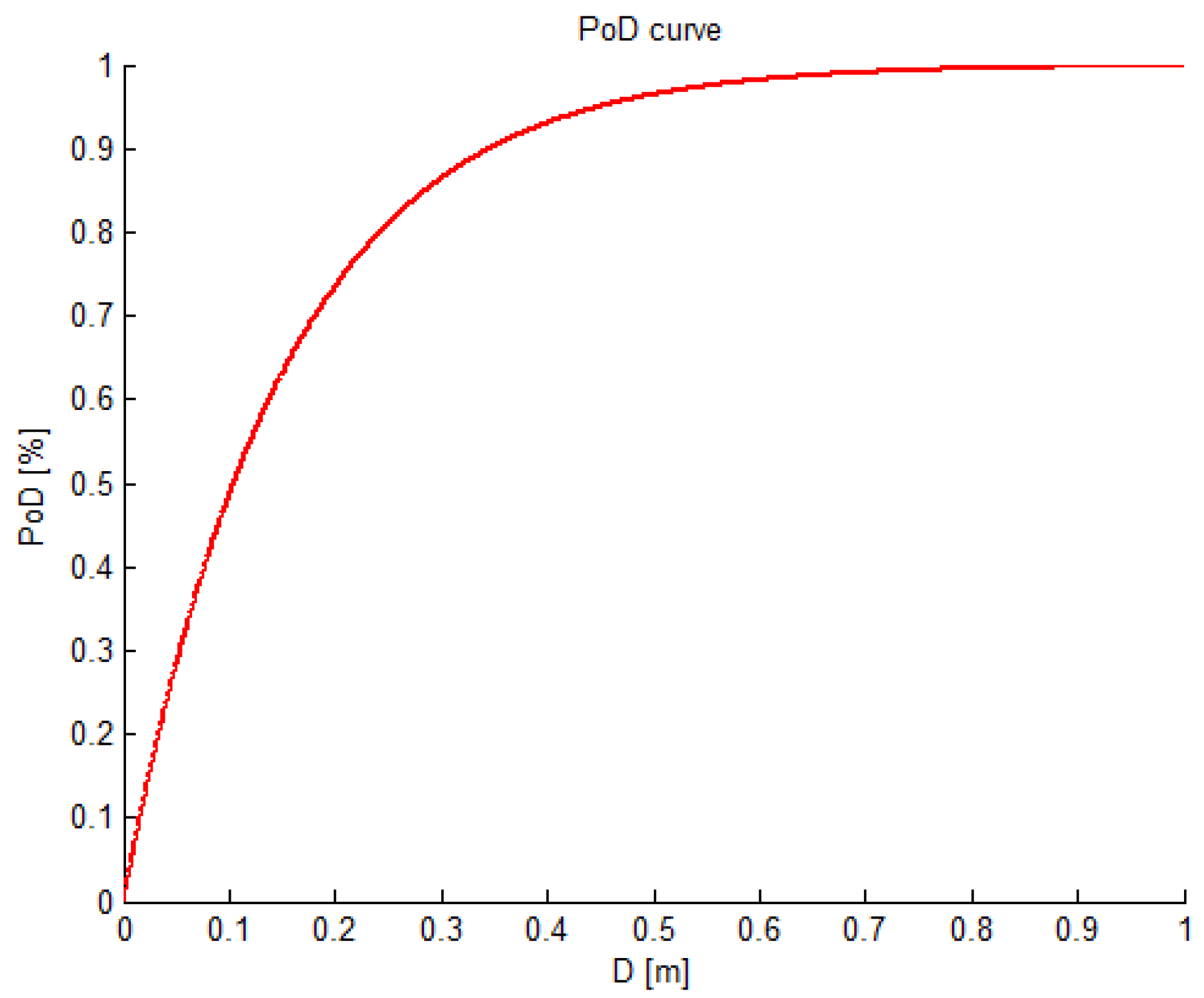
The inspection model considers the scheduled inspection time, the duration for an inspection and the probability that an inspection is successful. This is modeled using the probability of detection (PoD) curve as a function of the damage size D, modeled in this case by a crack length noted a. The PoD curve is obtained Equation (3), taken from [4].

$$PoD\left(D\right)=P_0\left(1-exp\left(\frac{-D}{\text{λ}}\right)\right)$$

(3)

The maximum probability of detection, P₀ (for very large amounts of damage) and the expected value of the smallest detectable damage, λ are set to 1 and 0.2, respectively. These parameters are dependent on the inspection method that is being considered. For this study, the values are chosen for illustrative purposes and do not reflect a particular inspection procedure. Figure 3 shows the probability of detection (PoD) curve corresponding to these values.

Figure 3. Probability of detection curve.

Figure 3. Probability of detection curve.

In reality, a probability of false indication also exists. While this is not taken into consideration in this model, it is noted that false indications can lead to unnecessary maintenance interventions. Further, it is assumed for illustration that an inspection of the entire blade has a duration T_in of eight hours and, during this period, the turbine is stopped. This implies that, in addition to the cost of inspection, revenue losses are also present.

Inspections are assumed to take place at regular time intervals. The influence of this interval is studied in Section 4. Alternatively, inspection times can be optimized following the general model in Section 2.

3.5. Damage Model

In order to build a reliable damage model, a failure mechanism must first be considered so that its progression can be traced throughout the lifetime of the blade. However, identifying the failure mechanism of a turbine blade is not a trivial task, due to the complexity of the physical phenomenon itself and the limited amount of information available on blade fatigue behavior. [6] makes an attempt of identifying the initial causes that eventually lead to failure, by performing both numerical experiments and a full-scale static test on a 40-m turbine blade. It is concluded in the paper that “the aerodynamic shells debonding from the adhesive joints is the initial failure mechanism followed by its instable propagation which can lead to collapse” [6]. Therefore, although a detailed mechanism cannot be expressed, the damage model used in the present paper is based on the assumption that failure is achieved when cracks in the adhesive joints reach a certain length a_fail.

The model is contains three stages that are described in the following subsections:

• crack initiation at the start of the blade’s life
• damage propagation during the blade’s lifetime
• failure is achieved when a crack length reaches a_fail

The size and positions of the cracks at the beginning of the blades lifetime are unknown. This being the case, a random damage state is generated. The distances l1, l2 …. ln are generated from a Poisson process, with the intensity λ_p(l) and the size a of each crack being randomly generated using a lognormal distribution. The input example values for the crack size model are shown in Section 3.8.

The average number of cracks is set at 0.3 per meter length of the blade. It is noted that this model assumes cracks to be evenly distributed along the length of the whole blade. This may not be realistic, but other models with cracks concentrated in certain areas of the blade can easily be implemented.

Once the cracks are generated, their growth is modeled using a fracture mechanics approach, under the assumption of having one-dimensional cracks along the length of the blade.

The crack growth in the bondline is determined by the load cycles applied to the blade and the crack length at a given time. The crack growth is assessed for 10 min intervals following Paris law, as shown in Equation (4), taken from [7]:

$$\frac{da}{dt}= \frac{A{\left(\Delta K\right)}^m}{{\left(1-R\right)}^{m\left(1-{\text{λ}}_w\right)}}$$

(4)

da

  Increase in crack length

ΔK

  Stress intensity factor

Δt

  Time period

A,m,λ^w

  Material parameters

R

  Stress ratio

The stress intensity factor ΔK for a time interval Δt is determined as a function of the wind speed, the crack size and the load cycle distribution corresponding to Δt. The model is shown in Equation (5), taken from [8]:

$$\Delta K\left(u,I\right)=\underset{0}{\overset{\infty }{{\displaystyle \int }}}\Delta s f(\Delta s|u,I) \sqrt{\text{π} a} d\Delta s$$

(5)

Δs

  Load range

a

  Crack length

f(Δs|u,I)

  Density function of load cycles

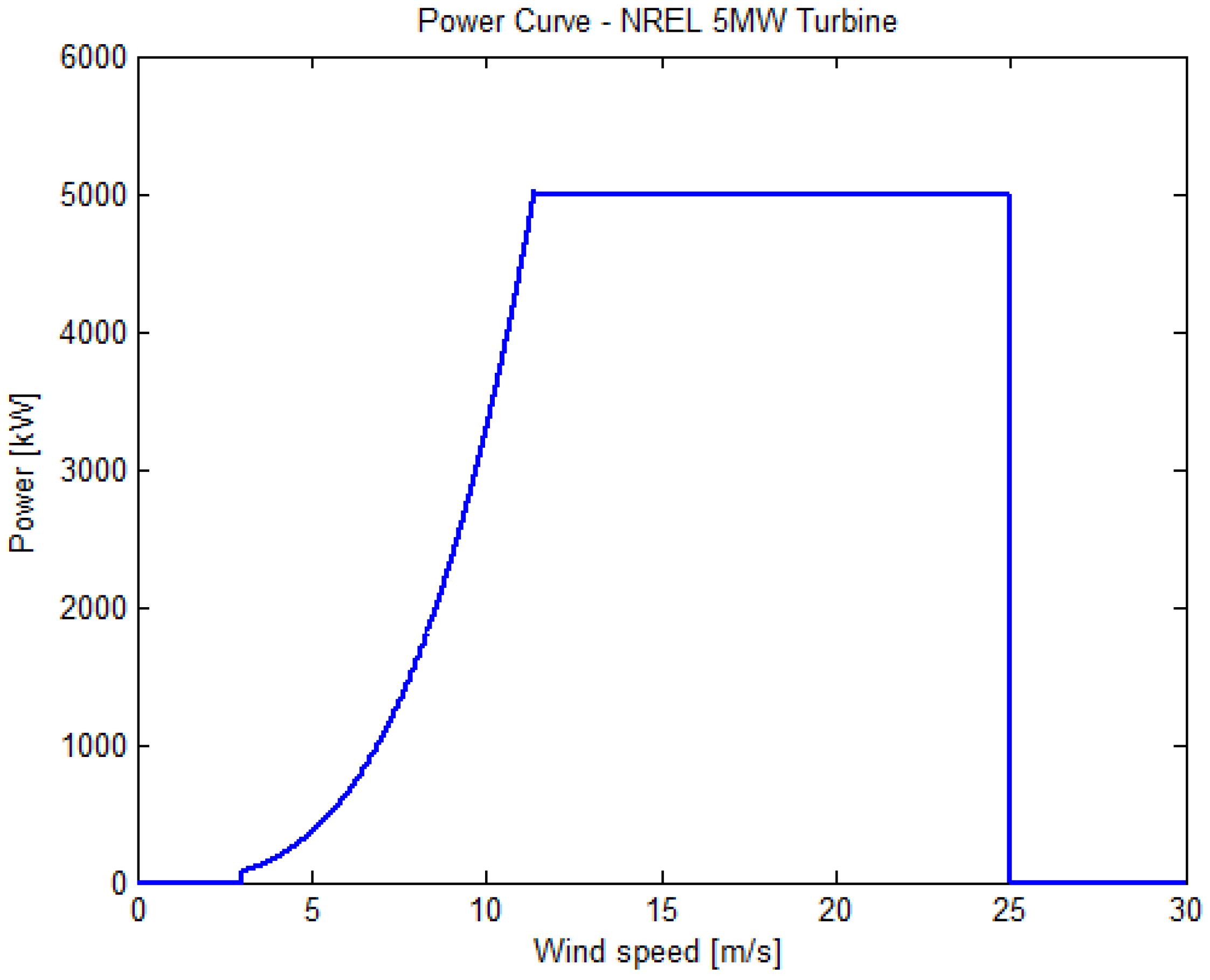
The statistical distribution function of the cycle ranges is dependent on the turbulence intensity for a given site and the mean wind speed. To determine the distribution of the load cycles as function of the environment, a series of 10-min simulations is made using the aero-elastic simulator FAST defined in [5], covering all operational wind bins of the turbine. Data is collected for the flap-wise blade bending moment for 1 m/s wind bins from cut-in to cut-out wind speed, using a reference turbulence intensity of 0.08, as determined for the weather data used from the platform location. It is noted that other loads, i.e., edge-wise bending, also contributes to the development of cracking, however, the model uses only flap-wise loading as it is considered to be the dominant load and sufficient for the study. To avoid large statistical uncertainties, 15 seeds are used for each wind bin.

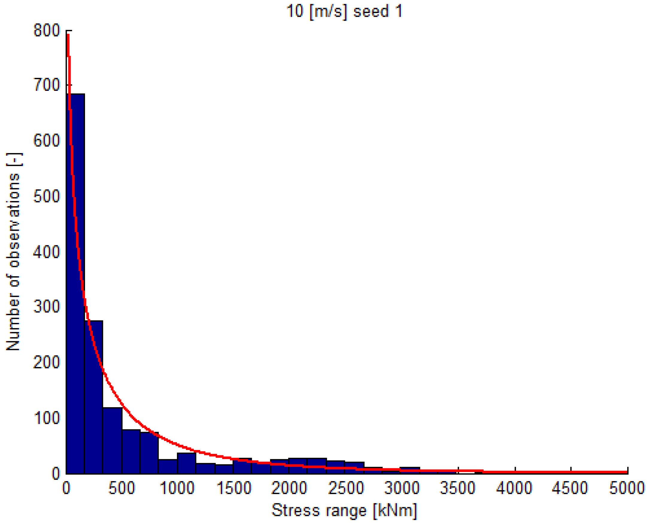
The following step is to determine the load range distribution for each wind bin as a function of the wind speed. This is done by using a rainflow count, after which the results are fitted to a two-parameter Weibull distribution. The cycle count for a 10 m/s wind bin, along with the fit is shown in Figure 4. Along with the stress ranges, the mean value of the cycle midpoints is determined in order to estimate the cycle ratio R.

Figure 4. Distribution of stress ranges in a 10 min simulation.

Figure 4. Distribution of stress ranges in a 10 min simulation.

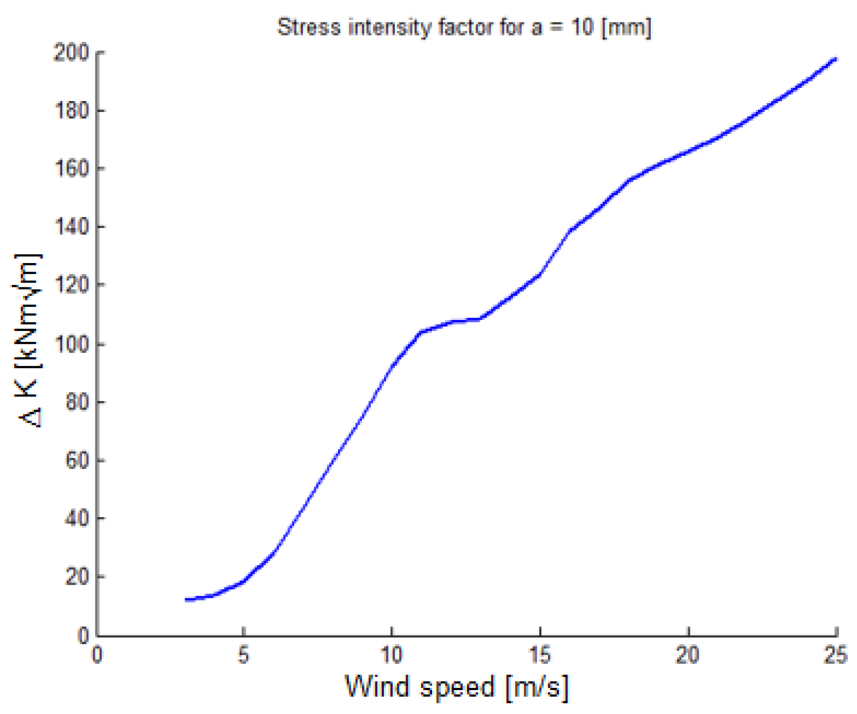
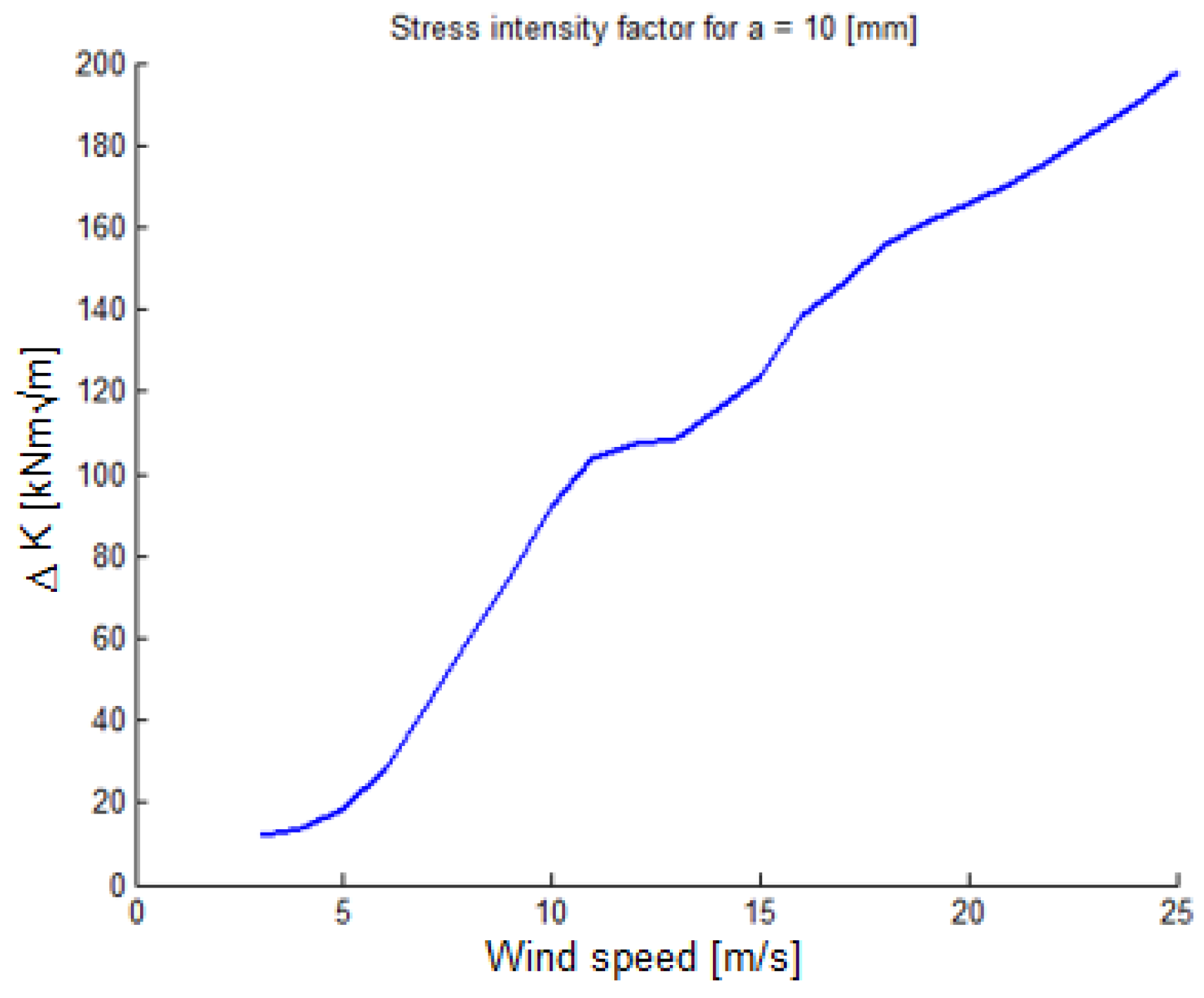
By integrating according to Equation (4), the stress intensity factor for a 10-min interval, given the wind speed, the turbulence intensity, and the crack size at the beginning of the time interval, is determined. This is shown in Figure 5, for a crack size of 10 mm.

Figure 5 illustrates the influence of the blade’s pitching mechanism, reducing the loads after a rated wind speed. Because the stress intensity factor is highly dependent on the crack size, its value is updated after every 10-min interval, according to Equation (5), considering the new crack size, determined with Equation (4).

Figure 5. Distribution of stress intensity factor.

Figure 5. Distribution of stress intensity factor.

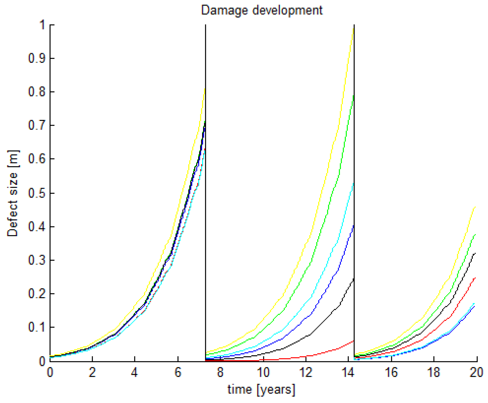
As stated previously, failure is assumed to occur when the cracks reach a certain value a_fail.

Figure 6 and Figure 7 show an example run of the damage model, illustrating all stages, for a_fail of 1 m. The randomly generated initial damage state is seen in Figure 6, while Figure 7 shows how the cracks develop during the lifetime of the blade.

Figure 6. Initial damage state.

Figure 6. Initial damage state.

Figure 7. Damage development and failure.

Figure 7. Damage development and failure.

Figure 7 shows the evolution of a number of cracks with different starting sizes, each shown with a different color. It is seen that when one of the cracks reaches the failure limit of 1 m, the blade is considered to be collapsed. This position is marked by the vertical line in figure 7. At this point, the development of all cracks is stopped and the blade is replaced with a new one, after which the process is repeated.

3.6. Repair Model

As stated above, the model considers both preventive/condition based and corrective type maintenance. A preventive repair is scheduled when a crack with a length greater than a certain value a_rep is successfully detected. The value of the repair limit is an important decision parameter and its influence will be analyzed in Section 4. In the event of a collapse, a corrective repair is performed. Both types of intervention are dependent on the transport vessels and if the weather conditions do not permit for an immediate intervention, the activity is postponed until an appropriate weather window appears.

The power loss is also estimated during the downtime of the turbine, considering both the duration of the repair itself and the downtime caused by inappropriate weather. The duration for each type of action is shown in Table 2.

Table 2. Repair duration.

Preventive	24 h
Corrective	72 h

Table 2. Repair duration.

Preventive	24 h
Corrective	72 h

In the case of a corrective repair, it is considered that the blade is replaced.

3.7. Cost Model

The cost model needs to cover cost of inspections, maintenance interventions and revenue losses as a result of downtime from each activity and eventual failure. Although it should be noted that cost models have a large influence on what an optimum maintenance plan will be, the following values (Table 3) are chosen for illustrative purposes.

Table 3. Cost.

Activity	Symbol	Value	Unit
Energy cost	CL	0.04	€/kWh
Inspection	CIN	2,500	€
Preventive repair	CREP	10,000	€
Corrective repair	CF	100,000	€

Table 3. Cost.

Activity	Symbol	Value	Unit
Energy cost	CL	0.04	€/kWh
Inspection	CIN	2,500	€
Preventive repair	CREP	10,000	€
Corrective repair	CF	100,000	€

3.8. Stochastic Model

The resulting total cost for a certain maintenance plan is highly susceptible to uncertainties in the input parameters. To account for this, a stochastic model is considered, as shown in Table 4, where the values were chosen so that the failure frequency of the blade is around 11 years, as observed in the industry [9].

Table 4. Stochastic model parameters.

Parmeter	Dist	Mean	COV
ain	LN	10	0.15	mm
A	LN	1.2−9	0.05	$\frac{1}{{\text{kN s m}}^{1/2}}$
m	N	1.8	-	-
λw	N	0.8	0.05	-

Table 4. Stochastic model parameters.

Parmeter	Dist	Mean	COV
ain	LN	10	0.15	mm
A	LN	1.2−9	0.05	$\frac{1}{{\text{kN s m}}^{1/2}}$
m	N	1.8	-	-
λw	N	0.8	0.05	-

4. Results and Discussion

With the model setup described in the previous section, a study of the main maintenance decision parameters can be performed with the goal of optimizing the expected total cost of O&M.

Two different sets of simulations are performed, considering perfect and imperfect repairs.

4.1. Inspection Interval

Inspection activities are the main tool in determining whether or not a blade needs to undergo a repair, potentially saving considerable expenses by avoiding future corrective repair. However, if the interval between two consecutive inspections is too small, it can lead to unnecessary high maintenance costs.

The optimum time between inspections is found as the time interval where the total expected preventive and corrective maintenance cost is minimized. The optimum interval is also dependent on the reliability of the inspection, as described in Section 3.4. The cost functions, for the example described in this paper, are shown in Figure 8a,b, considering a repair limit of 10% of the failure limit. Imperfect repairs imply that a repaired crack is not completely eliminated, but is reduced to a random value in the initial crack distribution, described in Table 4. This is meant to account for ongoing development of new cracks during the life of the blade, which is not modeled otherwise, while perfect repairs imply a complete removal of any repaired crack.

Figure 8. Inspection interval, (a) perfect repairs; (b) imperfect repairs.

Figure 8. Inspection interval, (a) perfect repairs; (b) imperfect repairs.

A clear minimum point is seen at a time interval of two years for both assumptions. Below this point, the amount of preventive maintenance and the associated cost is unnecessarily high, due to the low risk of failure, as illustrated by the corrective cost function. On the other hand, choosing a larger time interval increases the chances of collapse, greatly raising the expected corrective cost, as well as the revenue loss.

Although the trend of the total cost is similar in both analyses, indicating an optimal interval of around two years, the difference in magnitude is evident. This is especially noticeable when looking at the preventive maintenance component.

The reason for this is that, when perfect repairs are assumed together with a small inspection interval, all existing cracks are fixed within the beginning of the blade’s lifetime, leaving it in a perfect health state. Because the model analyzes existing cracks and does not account for development of new cracks, no further repairs will be required during the rest of the blade’s life, resulting in a relatively low maintenance cost.

In contrast, when imperfect repairs are considered together with a small inspection interval, crack growth will be present during the entire life of the blade, due to the fact that they are not entirely removed. This implies a larger number of preventive repairs, as is seen in the cost function shown in figure 8b. The corrective cost for small inspection intervals is similar with the case of perfect repairs, due to the low probability of collapse.

When changing to high values for the inspection interval, the situation is reversed. The increased probability of failure is evident in the corrective cost function, while the preventive cost converges to around the same value as in the case for perfect repairs.

4.2. Repair Limit

The decision on the repair limit has a strong influence on both the amount of preventive maintenance and the risk of corrective repair. By choosing a high limit, the degradation state is allowed to approach the failure limit, raising the risk of a collapse event. On the other hand, repairing damage on sight (i.e., low repair limit) raises the amount and cost of preventive maintenance by wasting significant portions of the blade’s remaining life.

The cost functions as a function of repair limit are shown in Figure 9a,b. for an inspection time interval of two years.

The cost functions are dependent on the cost of repair, transportation, and energy, as well as on the reliability and frequency of inspections. In both cases, the results indicate that a repair limit less than 40% is optimal.

The same difference in the magnitude of the cost components that was described in the previous section is observed.

A low intervention limit implies a larger number of repairs, given that cracks are continuously present during the entire lifetime of the blade. This is seen in the difference between the preventive cost functions in the figure 9a,b at intervention limit values between 10% and 40%. At values over 50%, the probability of requiring more than one preventive repair is low, leading to a similar expected cost for both assumptions.

Figure 9. Repair limit, (a) perfect repairs; (b) imperfect repairs.

Figure 9. Repair limit, (a) perfect repairs; (b) imperfect repairs.

The opposite can be said about the corrective cost component. Low intervention levels greatly reduce the probability of requiring more than one blade replacement, resulting in a relatively close expected cost for corrective repair for both assumptions. The difference increases along with the failure probability, i.e., the intervention limit.

In addition to the evident difference in magnitude, the trends for both models are similar, indicating an optimal intervention limit of under 30%.

The risk-based maintenance model, as described in [3], is used in this paper together with a physical degradation model for wind turbine blades to assess the impact of different maintenance decisions.

The focus of the model is on identifying a failure mechanism for the blade and modeling the degradation based on weather measurements.

The model can be improved and adapted to various types of blades used in the industry by coupling it with information from destructive/non-destructive tests. Knowledge of initial imperfections in the bonding material, crack propagation, and limit of failure can greatly reduce epistemic uncertainties in the model. Statistical knowledge, such as failure rates, can also help perfect the calibration.

A complex naval logistics and cost model were not in the scope of this paper, therefore they are reduced to fixed values for both preventive and corrective maintenance activities, and do not account for the rate of interest. Ideally, various transport possibilities should be taken into account, each with its own limitations and costs. An example using the same risk-based framework can be found in [4].

5. Conclusions

In this paper, the degradation of an offshore turbine blade’s adhesive joint was modeled using fracture mechanics and used together with a risk-based maintenance decision framework to optimize lifetime cost, with respect to inspection frequency and repair limit.

A clear influence of the two decision parameters, interval between inspections, and intervention limit, has been found for each cost component, thus, highlighting the optimal value for the setup described in the paper. Predominant cost components have been identified, showing large expenses from corrective maintenance and revenue losses for a reduced frequency of preventive maintenance.

The model can potentially be improved to quantify cost sensitivity to various other parameters, such as logistics planning and different inspection methods. Furthermore, Bayesian statistical methods could be employed to update the damage propagation models using information on the observed damage indicators from condition monitoring.

References

1. Wouter, E.; Obdam, T.; Savenije, F. Current Developments in Wind—2009; Technical Report for Energy Research Centre of The Netherlands: Petten, The Netherlands, 2009. [Google Scholar]
2. Chou, J.-S.; Tu, W-T. Failure analysis and risk management of a collapsed large wind turbine tower. Eng. Fail. Anal. 2011, 18, 295–313. [Google Scholar]
3. Sørensen, J.D. Framework for risk-based planning of operation and maintenance for offshore wind turbines. Wind Energy 2009, 12, 493–506. [Google Scholar]
4. Nielsen, J.J.; Sørensen, J.D. On risk-based operation and maintenance of offshore wind turbine components. Reliab. Eng. Syst. Saf. 2011, 96, 218–229. [Google Scholar]
5. Jonkman, J.M.; Buhl, M.L., Jr. FAST User’s Guide; Technical Report for National Renewable Energy Laboratory: Golden, CO, USA, 2005. [Google Scholar]
6. Yang, J.; Peng, C.; Xiao, J.; Zeng, J.; Xing, S.; Jin, J.; Deng, H. Structural investigation of composite wind turbine blade considering structural collapse in full-scale static tests. Compos. Struct. 2013, 97, 15–29. [Google Scholar] [CrossRef]
7. Stephens, R.I.; Fatemi, A.; Stephens, R.R.; Fuchs, H.O. Metal Fatigue in Engineering; John Wiley & Sons: Hoboken, NJ, USA, 2001. [Google Scholar]
8. Sørensen, J.D.; Frandsen, S.; Tarp-Johansen, N.J. Effective turbulence models and fatigue reliability in wind farms. Probab. Eng. Mech. 2008, 23, 531–538. [Google Scholar]
9. Faulstich, S.; Hahn, P.; Tavner, P. Wind turbine downtime and its importance importance for offshore deployment. Wind Energy 2011, 14, 327–337. [Google Scholar] [CrossRef]