The Use of a Statistical Model of Storm Surge as a Bias Correction for Dynamical Surge Models and its Applicability along the U.S. East Coast

Abstract

The present study extends the applicability of a statistical model for prediction of storm surge originally developed for The Battery, NY in two ways: I. the statistical model is used as a biascorrection for operationally produced dynamical surge forecasts, and II. the statistical model is applied to the region of the east coast of the U.S. susceptible to winter extratropical storms. The statistical prediction is based on a regression relation between the “storm maximum” storm surge and the storm composite significant wave height predicted ata nearby location. The use of the statistical surge prediction as an alternative bias correction for the National Oceanic and Atmospheric Administration (NOAA) operational storm surge forecasts is shownhere to be statistically equivalent to the existing bias correctiontechnique and potentially applicable for much longer forecast lead times as well as for storm surge climate prediction. Applying the statistical model to locations along the east coast shows that the regression relation can be “trained” with data from tide gauge measurements and near-shore buoys along the coast from North Carolina to Maine, and that it provides accurate estimates of storm surge.

1. Introduction

Storm surge is a potentially devastating rise in the coastal water levels caused by tropical cyclones such as hurricanes and typhoons and by extratropical storms. Approximately 50% of the world’s population lives within 150 kilometers of the ocean, particularly in low-lying coastal areas susceptible to the consequences of storm surge. Although tropical cyclones, with their lower low-pressure centers and higher wind speeds, typically produce significantly higher surge than extratropical cyclones do (Hurricane Katrina in the U.S. in 2005, for example), extratropical cyclones are frequent occurrences during much of the year over large populated coastal regions such as the east coast of the United States, and therefore require similar research efforts and accurate prediction. These extratropical storms occur on average 10–12 times per year and the strongest and most destructive storms appear on average 2 to 3 times per year [1,2]. Storm surge can lead to large loss of human life, destruction of homes and civil infrastructure, and disruption of commerce. The Fifth Assessment Report of the Intergovernmental Panel on Climate Change (IPCC) [3] estimates that over the next century global sea level is likely to rise from between 26 and 63 cm, and, depending on emissions, as much as 90 cm. This sea level rise will extend the zone of impact from storms, storm surge, and storm waves farther inland. Examples of extratropical storms and their associated damage along the east coast abound. The extratropical storm of 11–12 December 1992 [4] produced near-record flooding along the entire Atlantic Coast. Storm surge levels of over 1 meter persisted for a few days at Sandy Hook, NJ, with a maximum storm surge value of 2.13 m [4]. The storm surge for that storm recorded at The Battery, NY, was 1.75 m [5]. Flooding resulted in the closing of major highways and railroads, in millions of dollars of losses due to property damage, and in two storm-related deaths. For reference, a storm surge threshold value of 0.6 m (above Mean High Water Level) can cause minor flooding during a high tide at The Battery, NY, and is often used as a criterion to issue an advisory of coastal flood conditions for the New York Metropolitan region by the National Weather Service [6]. More recently, on 15–16 April 2007, an extratropical system resulted in storm surge at The Battery, NY, of 1 m [7]. In addition to flooding, power outages, property damage, evacuations and traffic disruption, there were several deaths reported for this storm.

The factors that contribute to the challenge of modeling and predicting storm surge include storm intensity and storm track, coastal bathymetry, pre-storm average water height, astronomical tides and ocean wave field and associated wave transport. The National Oceanic and Atmospheric Administration (NOAA) produces 96-hour operational surge forecasts with the extratropical storm-surge model called ET-SURGE (ETSS) developed by Kim et al. [8]. A detailed description of the ETSS model output fields is available online at [9]. The operational storm surge forecast guidance consists of the ETSS output augmented by a bias correction. This error correction is computed as the five-day average of the difference between the observed and the predicted water levels, computed over the 5 days previous to the forecast start time and referred to as the “anomaly” [9]. This constant is added to the entire forecast produced by the dynamical model. NOAA now also provides surge forecast guidance from 96-hour surge forecasts using the Extratropical Surge and Tide Operational Forecast System (ESTOFS) [10], which demonstrates error characteristics that are comparable to the bias-corrected ETSS [11], but has been operational for a short period of time and will not be discussed here. Despite recent advances in the development of dynamical models such as ETSS and ESTOFS and advances in computational capability, however, forecast errors remain quite large and improvements in performance are needed [6].

A time series of the NOAA bias correction (not shown) depicts significant temporal variability. This suggests that the existing method of bias correction is limited to near-future events and times (probably out to a few days), and could not be used, for example, to correct surge forecasts out to two weeks using the 14 day forecasts regularly released by many numerical weather prediction centers (see for example [12]), or to correct surge forecasts based on future climate projections. Both of these goals are desirable and feasible, and have motivated studies of hurricane-related storm surge [13,14]. Similar studies for extratropical storm surge have not been reported despite the indications from many Coupled Model Intercomparison Project—5 (CMIP5) climate forecasts that the frequency and intensity of extratropical storms may increase in a warmer climate [15].

There are other existing methods to correct errors in dynamical surge forecasts using observed water level data. For example the German Federal Marine and Hydrographic agency uses a Model Output Statistics (MOS) approach [16]. This approach produces a modified water level and surge time series based on a regression model. The regression includes over a dozen predictors, the most important of which are the dynamical model output itself and recent error in surge forecast. The evaluation of this technique shows substantial reduction in forecast error for lead times up 24 h. There was little to no benefit from the MOS approach after 33 h lead time. Based on these results we infer that, like NOAA’ surge correction, this approach would also not be beneficial for long lead time surge forecasts.

Part I of the present study describes an improved bias correction method for use in operational storm surge forecasts that may not have the issue of degrading skill for long lead time forecasts. The new bias correction makes use of the statistical model developed by Salmun et al. [2] to predict the maximum value of storm surge during a storm event which is referred to as the “storm maximum storm surge” (SSMAX). The model was validated for surge forecasts by Salmun et al. [17]. SSMAX is an event based metric for each storm event. A storm event is defined by the period over which the sea level pressure (as measured at a nearby location) remains below two standard deviations from its seasonal mean. The authors presented a regression equation relating the value of SSMAX at The Battery, NY, to the average of the top one-third of significant wave heights during the storm event measured at the National Data Buoy Center (NDBC, [18]) station off Fire Island, NY (NDBC Sta. 44025). The regression relation was developed based on storm surge computed from water level available for The Battery, NY [5], for the extratropical storm season during the period 1991–2008. The statistical model based on the storm composite significant wave height was chosen for its simplicity since the model with this single predictor was shown to perform as well as models with up to seven different predictors. The regression relation they obtained was:

$$SSMA{X}_{44025}= 0.2055H_{44025}- 0.0851$$

(1)

with RMS error of 0.167 m. $H_{44025}$ denotes the significant wave height at NDBC Sta. 44025. The capability for predictions of the maximum value of the storm surge due to a storm event by the statistical method was verified for The Battery, NY, based on a series of retrospective forecasts using predicted wave heights from NOAA’s WAVEWATCH III™ (WWIII) wave model [19] for storm events determined from surface pressure from NOAA’s North American Mesoscale (NAM-WRF) [20] weather forecast model [8]. Salmun et al. [17] showed that the prediction capability of the statistical model is comparable to that of NOAA’s operational forecast of the storm maximum storm surge.

The relationship between the height of waves and the magnitude of the storm surge that is reflected in the regression relation can be conceptualized in terms of basic physical processes. The wave field in the ocean is the result of energy transfer from the wind field to the surface. The transfer depends strongly on wind velocity, wind duration and the distance affected by sustained winds or fetch. Significant wave heights are determined largely by the energy imparted to the water over the fetch, hence they are a good indication of the intensity of the winds (storm) that produced them. SSMAX represents a single value, the maximum, of storm surge that is experienced at a location during the entire period of a storm and as such SSMAX does not give information about timing of the potentially most damaging storm surge. Its usefulness derives from its simplicity, from being easy to compute and from its ability to capture local information about a storm from a near-shore single location. Although the prediction of an event-based storm maximum storm surge does not entirely satisfy the public’s need for surge forecasting, an accurate prediction of SSMAX can provide valuable information, and can be used in conjunction with NOAA’s dynamical forecast to provide better operational forecasts. In addition, because SSMAX makes use of statistical relationship between the state of the ocean and the surge there should be fewer restrictions in the use of SSMAX as a bias correction related to forecast lead time.

In Part II of the present work we examine the applicability of the statistical model to the other areas along the U.S. east coast. In this way we examine the extent to which the local geography and geomorphology affect the specifics of the relationship between the significant wave height measured at a local buoy and SSMAX. Following this introduction, the statistical storm surge model and its validation are briefly described. In Section 3 we describe, discuss and evaluate the use of SSMAX as a bias correction to current NOAA storm surge forecast. The extension of the statistical method for storm maximum storm surge estimated along the North Atlantic east coast affected by extratropical systems is presented in Section 4 and Section 5 summarizes the major results of the study and Section 6 discusses the present findings and future extensions of the study.

2. Description of the Statistical Method

A brief summary of the relevant details of the statistical method of Salmun et al. [2,17] and the choice of storms used for its evaluation is presented here. Salmun et al. [2] established a statistical relation between the maximum value of the surge (SSMAX) reached during any particular storm event and the storm composite near-shore significant wave height. Values of SSMAX were computed using water level data at The Battery, NY, obtained from NOAA’s Center for Operational Oceanographic Products and Services (CO-OPS) [5], and nearby significant wave heights were determined from data measured at the National Data Buoy Center (NDBC, [18]) Sta. 44025 for extratropical storm events during the storm season (September–April) of the period 1991–2008. The storm composite significant wave height is defined as the average of the “top third” largest significant wave heights during the storm period. Extratropical storm events were determined using a threshold of two standard deviations below the climatological mean of the sea level pressure time series, also using data from the NDBC station. A single event that satisfied this sea level pressure criterion, lasted longer than four hours and was separated from all other continuous groups of measurements by at least 24 hours defined a storm event. Extensive examination of surface weather maps was used to validate the list of storms.

Salmun et al. [17] tested the statistical method by performing a series of retrospective forecasts of the events identified by the earlier study that occurred during the period from February 2005 to December 2008. They used existing operational forecasts of surface pressure from NOAA’s North American Mesoscale (NAM-WRF) [20] weather forecast model, operational forecasts of wave height from NOAA’s WAVEWATCH III™ (WWIII) model [19] and the regression relation obtained by Salmun et al. [2]. The list of storms identified at NDBC station 44025 as described above for the test period was the starting list of candidate events for the testing process. Retrospective forecasts of sea level pressure, available at three-hour time intervals, were then used to verify the existence of candidate events in the forecast record. Any storm not forecasted was eliminated from the final list of test storms (which resulted in the elimination of one storm from the original record), and 41 storms comprised the testing sample. Starting and ending times for each storm event were determined from the forecasted sea level pressure. Storm composite significant wave heights at the NDBC station were computed based on retrospective forecasts from [19] for each storm event, and used as the predictor for SSMAX at The Battery, NY, USA.

The statistical predictions of SSMAX thus obtained were compared to values of “storm maximum” storm surge obtained from the NOAA ETSS model output, from the NOAA operational (bias corrected) forecasts, and from the observations at that location for each storm event. The results of this evaluation showed that the mean error of the statistical method for 12-, 24- and 48-h lead time forecasts is smaller than the mean error of the ETSS model forecasts with 95% confidence and that the predictions made with the statistical method are statistically indistinguishable from the NOAA bias-corrected operational forecast, which is the ETSS output with an anomaly correction.

3. Part I—The Statistical Approach as a Bias Correction

The statistical event-based forecast of SSMAX is used here to perform a bias correction for the duration of a forecasted storm event, and applied at each time during the storm event in a manner similar to the ETSS anomaly correction. This type of correction could be used during any storm event for which forecasts of sea level pressure and wave heights are available. We applied this approach to the ETSS forecasts of all storm events considered by Salmun et al. [17] in their study of storm surge at The Battery, NY. The use of the statistical model as a bias correction is evaluated here for the NOAA ETSS forecast, but could be used in a similar manner as part of a multi-model ensemble surge forecast, such as the one advocated by Di Liberto et al. [21].

The SSMAX predicted by the statistical model was used to correct ETSS model forecast by adding a constant value computed as the difference between the statistical prediction of SSMAX ($SSMA{X}_{stat}$) and the ETSS prediction of SSMAX ($SSMA{X}_{model}$). For each time during a particular storm event, we denote the corrected time series by $E{T}_{stat}$ and we write:

$$E{T}_{stat}\left(i,j\right)= ETS{S}_{model}\left(i,j\right)+ \left(SSMA{X}_{stat}\left(j\right)-SSMA{X}_{model}\left(j\right)\right)$$

(2)

where i refers to time during a particular event and j refers to the storm event number. The test cases used for evaluation here are the 41 storm events identified between 2005 and 2008 as described in Section 2. The simplest implementation of the bias correction is to apply the correction uniformly over the duration of the storm event as was done here. More complex weighting functions were attempted but found to underperform relative to the constant weighting and so are not justified. The corrected event time series, $E{T}_{stat}$, and the event time series corrected with NOAA anomaly, denoted by $E{T}_{anom}$, were compared to observations (OBS) at The Battery, NY, for each storm event. 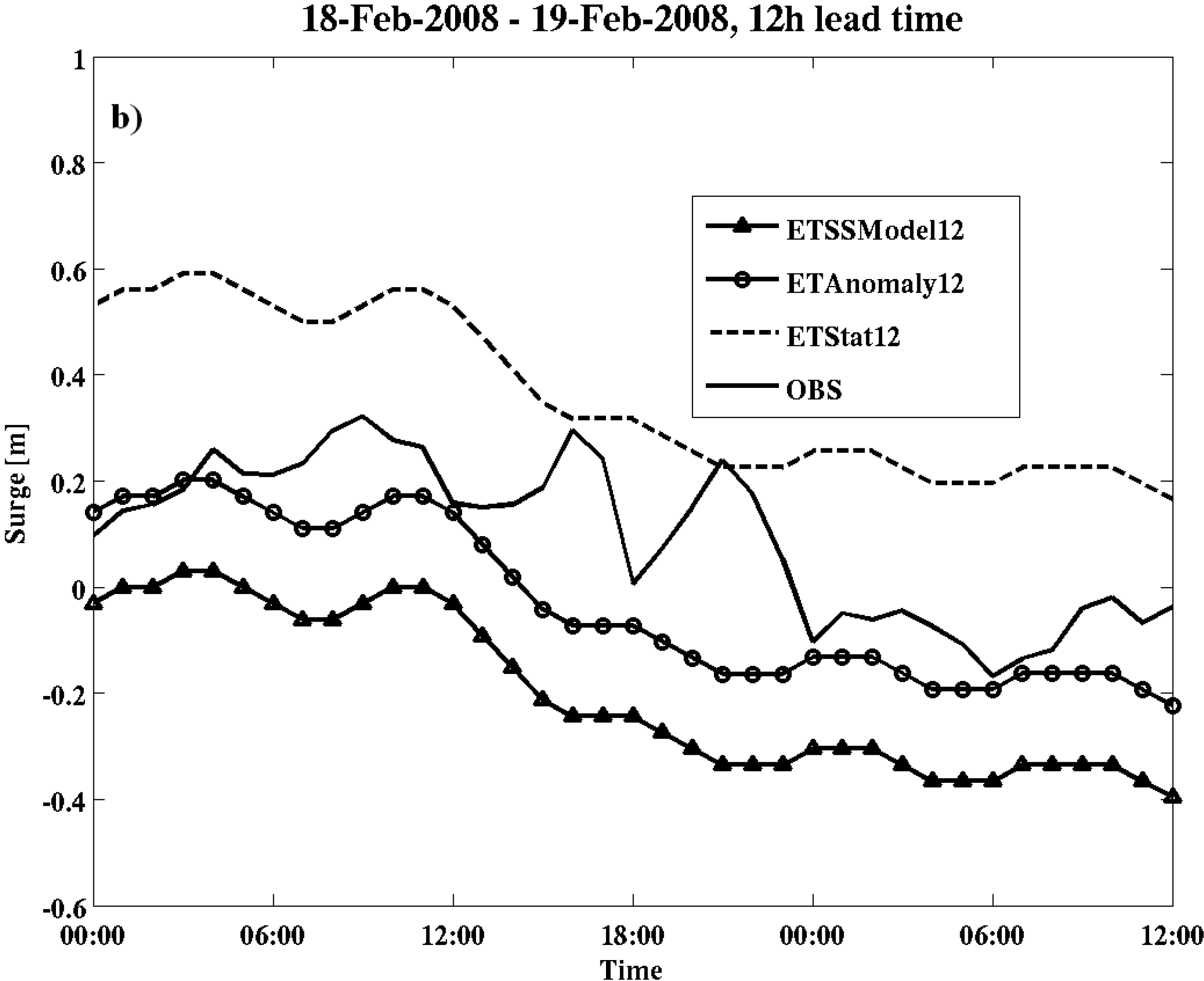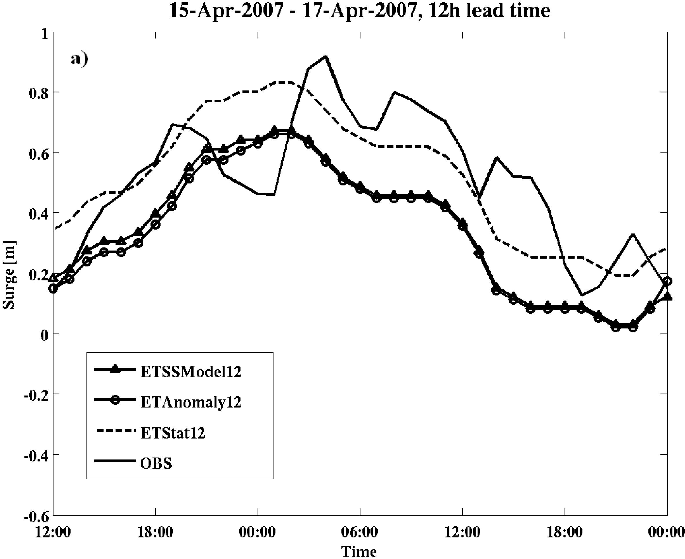Figure 1 shows the comparison among the different surge predictions for two typical storm events. Figure 1a shows the time series of a storm for which $E{T}_{stat}$ is higher than $E{T}_{anom}$, and closer to the observed surge. This occurred in approximately one third of the storm events, and is consistent with the determination made in Salmun et al. [17] that NOAA’s ETSS generally underpredicts surge. Figure 1b shows the time series of a storm for which $E{T}_{stat}$ is higher than $E{T}_{anom}$ and further away from the observed surge. This also occurred in approximately one third of storm events. Many of these storms were those for which Salmun et al. [17] determined that the error in the SSMAX forecasts was attributable to errors in the predicted wave heights rather than to a failure of the regression.

Means and standard deviations of the differences between each of the estimates and observations were computed for 12 h, 24 h and 48 h lead-time forecasts for each storm event. Lead-time was measured as the time elapsed between the forecast initial condition and the onset of the storm event, and the average storm event duration was 22.5 h, with a standard deviation of 19.1 h. Results for the means are summarized in Table 1. The variance of ($E{T}_{stat}-OBS$) is the same as the variance of $(ETS{S}_{model}-OBS$) by definition, and almost identical to the variance of ($E{T}_{anom}-OBS$). For the 12 h and 24 h lead-time forecasts, the mean difference between $E{T}_{stat}$ and OBS and the mean difference between $E{T}_{anom}$ and OBS are statistically indistinguishable as determined by a Student’s t-test, while at the 48 h lead-time the forecast using $E{T}_{stat}$ yields statistically more accurate results.

Figure 1. Hourly time series of storm surge from tide gauge observations and different model estimates. Solid black line is the gauge observations, dashed line is NOAA extratropical storm-surge model (ETSS) 12 h forecast with our statistical correction, the line with circles is NOAA ETSS 12 h forecast with NOAA’s anomaly correction, and the line with triangles is NOAA ETSS 12 h forecast. (a) Time series from storm 26 of Salmun et al. [17] beginning on 15 April 2007 12Z; (b) Time series from storm 30, beginning on 18 February 2007 0Z.

Figure 1. Hourly time series of storm surge from tide gauge observations and different model estimates. Solid black line is the gauge observations, dashed line is NOAA extratropical storm-surge model (ETSS) 12 h forecast with our statistical correction, the line with circles is NOAA ETSS 12 h forecast with NOAA’s anomaly correction, and the line with triangles is NOAA ETSS 12 h forecast. (a) Time series from storm 26 of Salmun et al. [17] beginning on 15 April 2007 12Z; (b) Time series from storm 30, beginning on 18 February 2007 0Z.

Table 1. Means of the differences between National Oceanic and Atmospheric Administration (NOAA)’s storm surge predictions, $ETS{S}_{model}$, corrected with the statistical estimate, $E{T}_{stat}$, and with NOAA’s anomaly, $E{T}_{anom}$, respectively, and observations at The Battery, NY, USA, and for 12 h, 24 h and 48 h lead-time forecasts.

Lead Time	$E{T}_{stat}-OBS$	$E{T}_{anom}-OBS$	$ETS{S}_{model}-OBS$
12 h	0.1976 m	0.1499 m	0.2459 m
24 h	0.1622 m	0.1274 m	0.2020 m
48 h	0.1682 m	0.1826 m	0.2854 m

Table 1. Means of the differences between National Oceanic and Atmospheric Administration (NOAA)’s storm surge predictions, $ETS{S}_{model}$, corrected with the statistical estimate, $E{T}_{stat}$, and with NOAA’s anomaly, $E{T}_{anom}$, respectively, and observations at The Battery, NY, USA, and for 12 h, 24 h and 48 h lead-time forecasts.

Lead Time	$E{T}_{stat}-OBS$	$E{T}_{anom}-OBS$	$ETS{S}_{model}-OBS$
12 h	0.1976 m	0.1499 m	0.2459 m
24 h	0.1622 m	0.1274 m	0.2020 m
48 h	0.1682 m	0.1826 m	0.2854 m

4. Part II—Statistical Technique Applied along the East Coast of the U.S

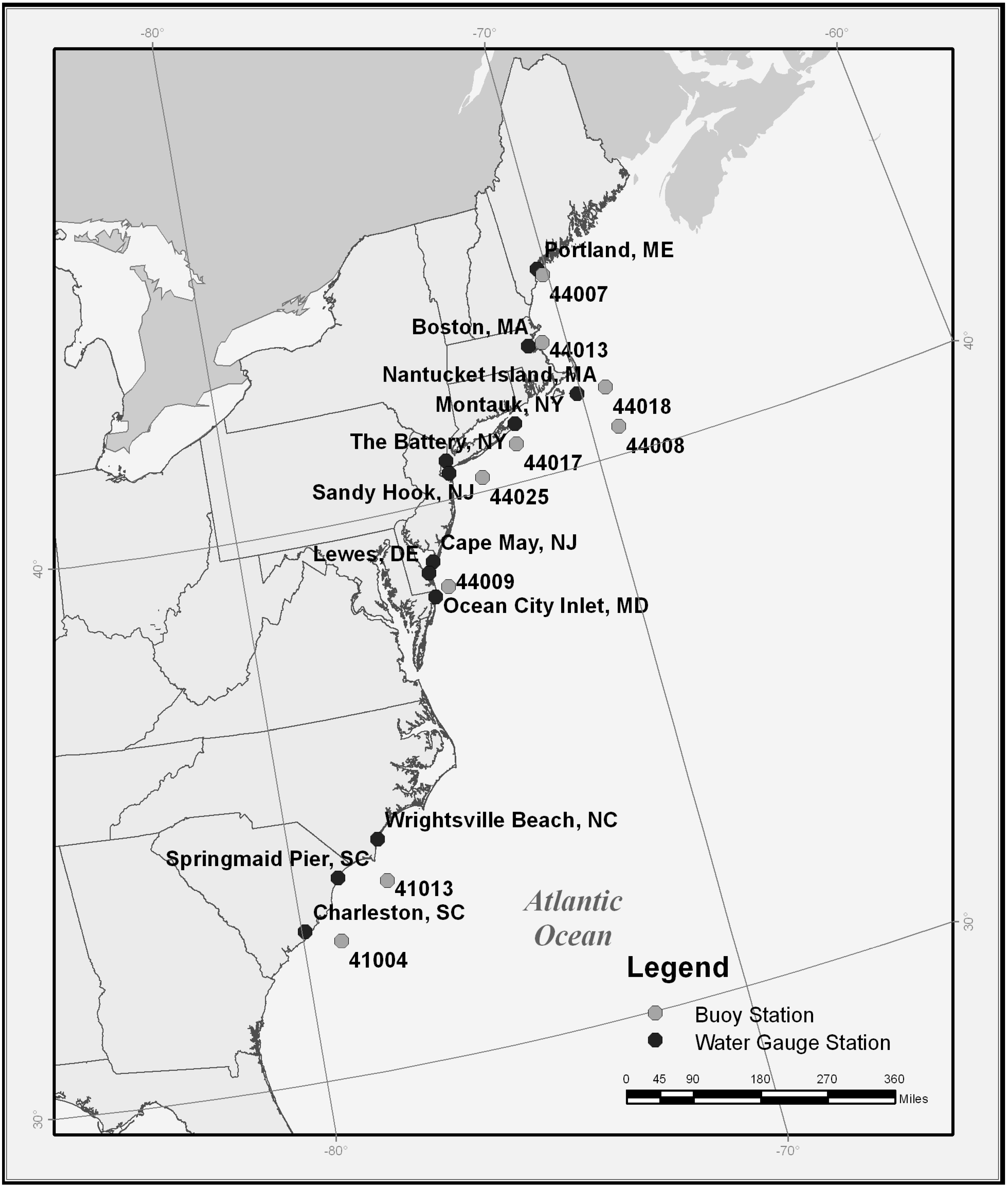
Extratropical storms affect a large portion of the U.S. east coast and the validity of any statistical method must be evaluated throughout. The region affected by East Coast Winter Storms chosen here was similar to the region defined in Hirsh et al. [1] and extends from Portland, ME, to Charleston, SC. Data from thirteen NOAA tide gauge stations and nine NDBC [20] buoys were selected for analysis and are indicated on the map in Figure 2 and listed and described in Table 2 and Table 3. The observed storm surge data were calculated using water level data from NOAA CO-OPS [5], and details of the computation can be found in Colle et al. [6]. Data from NDBC buoys were examined if the historical record ending in 2010 included at least five years of consecutive meteorological and oceanic data measurements. Data availability for the buoys ranges from 8 to 30 years, as seen in column 4 of Table 3. The buoys in this study are located on the continental shelf at 23.5 to 65.8 m water depth.

Table 2. List of tide gauge stations along the east coast of the U.S., their reference number, their location and a brief description of the specifics of their location.

Tide Gauge Station	Station #	Location	Description of Location
Portland, ME	8418150	43.66 N 70.25 W	South corner on the off shore end of the Maine State Pier
Boston, MA	8443970	42.35 N 71.05 W	Deep within the Boston Harbor near Logan International Airport
Nantucket Island, MA	8449130	41.28 N 70.10 W	Lee side of the island, inside a small harbor
Montauk, NY	8510560	41.05 N 71.96 W	Fort Pond Bay on the northern side of the Montauk peninsula at the entrance to the Long Island Sound
The Battery, NY	8518750	40.7 N 74.02 W	Deep within the Upper Bay of the New York/New Jersey Harbor
Sandy Hook, NJ	8531680	40.47 N 74.01 W	Just inside the Lower Bay (southern side of its entrance to the Lower Harbor), on the inside of the spit
Atlantic City, NJ	8534720	39.36 N 74.42 W	On a pier extending out from the barrier island
Cape May, NJ	8536110	38.97 N 74.96 W	Two tide gauges about 25 km apart, across the entrance to the Delaware Bay just behind the northern and southern points that form the entrance to the bay.
Lewes, DE	8557380	38.78 N 75.12 W
Ocean City Inlet, MD	8570283	38.33 N 75.09 W	55 km south of the Delaware Bay just inside a small inlet between two barrier islands
Wrightsville Beach, NC	8658163	34.21 N 77.79 W	Two tide gauges on piers extending out from barrier islands
Springmaid Pier, SC	8661070	33.65 N 78.92 W
Charleston, SC	8665530	32.78 N 79.93 W	On the Cooper River near the Port of Charleston

Table 2. List of tide gauge stations along the east coast of the U.S., their reference number, their location and a brief description of the specifics of their location.

Tide Gauge Station	Station #	Location	Description of Location
Portland, ME	8418150	43.66 N 70.25 W	South corner on the off shore end of the Maine State Pier
Boston, MA	8443970	42.35 N 71.05 W	Deep within the Boston Harbor near Logan International Airport
Nantucket Island, MA	8449130	41.28 N 70.10 W	Lee side of the island, inside a small harbor
Montauk, NY	8510560	41.05 N 71.96 W	Fort Pond Bay on the northern side of the Montauk peninsula at the entrance to the Long Island Sound
The Battery, NY	8518750	40.7 N 74.02 W	Deep within the Upper Bay of the New York/New Jersey Harbor
Sandy Hook, NJ	8531680	40.47 N 74.01 W	Just inside the Lower Bay (southern side of its entrance to the Lower Harbor), on the inside of the spit
Atlantic City, NJ	8534720	39.36 N 74.42 W	On a pier extending out from the barrier island
Cape May, NJ	8536110	38.97 N 74.96 W	Two tide gauges about 25 km apart, across the entrance to the Delaware Bay just behind the northern and southern points that form the entrance to the bay.
Lewes, DE	8557380	38.78 N 75.12 W
Ocean City Inlet, MD	8570283	38.33 N 75.09 W	55 km south of the Delaware Bay just inside a small inlet between two barrier islands
Wrightsville Beach, NC	8658163	34.21 N 77.79 W	Two tide gauges on piers extending out from barrier islands
Springmaid Pier, SC	8661070	33.65 N 78.92 W
Charleston, SC	8665530	32.78 N 79.93 W	On the Cooper River near the Port of Charleston

Table 3. List of the NDBC stations along the east coast of the U.S., their reference numbers, positions, water depths, length of the available data and number of storms identified at each station.

NDBC Station #	Location	Water Depth (m)	Length of Record (year)	Number of Storms
44007	43.531 N 70.144 W	23.7	30	366
44013	42.346 N 70.651 W	61	26	366
44018	41.255 N 69.305 W	63.7	10	132
44017	40.692 N 72.048 W	45	10	104
44025	40.250 N 73.166 W	36.3	21	254
44009	38.464 N 74.702 W	28	28	351
41013	33.436 N 77.743 W	23.5	8	89
41004	32.501 N 79.099 W	38.4	18	241

Table 3. List of the NDBC stations along the east coast of the U.S., their reference numbers, positions, water depths, length of the available data and number of storms identified at each station.

NDBC Station #	Location	Water Depth (m)	Length of Record (year)	Number of Storms
44007	43.531 N 70.144 W	23.7	30	366
44013	42.346 N 70.651 W	61	26	366
44018	41.255 N 69.305 W	63.7	10	132
44017	40.692 N 72.048 W	45	10	104
44025	40.250 N 73.166 W	36.3	21	254
44009	38.464 N 74.702 W	28	28	351
41013	33.436 N 77.743 W	23.5	8	89
41004	32.501 N 79.099 W	38.4	18	241

Figure 2. A reference map of the study area showing the locations of all tide gauges and National Data Buoy Center (NDBC) stations used in the analysis.

Figure 2. A reference map of the study area showing the locations of all tide gauges and National Data Buoy Center (NDBC) stations used in the analysis.

A regression analysis similar to that described in Salmun et al. [2] was performed for thirteen selected pairings of tide gauges and nearby buoys. The only new aspect of the regression analysis reported here is the use of non-dimensional wave heights as predictors (rather than actual wave heights, as was done in Salmun et al. [2]), designed to help assess the relative importance of the different terms in the regression. The values of wave heights were non-dimensionalized by the mean significant wave height computed over all events considered at a single location.

The choice of tide gauge—buoy pairs to use for the remainder of the regression analysis was informed by the “best performing” regression based on the magnitude of the root mean square error of the regression. Consideration for the selection of pairings was given to quality of data at the buoy, length of data record at the buoy, data record continuity, and proximity of the buoy to the location and setting (e.g., bay, barrier island) of the tide gauge. Based on these considerations, some tide gauges were initially paired with several different buoys, and the buoy that resulted in the smallest regression error was chosen for examination here. A list of the selected pairings appears in Table 4. The buoys selected are generally within 100 km of the tide gauge stations. For most pairings, the bearing (the angle between a line connecting buoy and tide gauge and a North-South line, measured from the North direction) from the buoy to the tide gauge is between 270° (buoy to the East of tide gauge) and 360° (buoy to the South of tide gauge). A notable exception is the bearing of 10.6° from NDBC Station 44017 to the tide gauge at Montauk, NY, USA.

Table 4. List of the tide gauge-NDBC station pairings selected in the study, the bearing from NDBC stations to tide gauges, distance separating them and the general orientation of the buoys with respect to the tide gauges, indicated in the fifth column as “dir to NDBC Sta”. Also shown in the table are the parameters of the regression equation for each pairing.

					Regression Equation
Pair	Tide Gauge	NDBC Station	Bearing—from NDBC Sta to WG (deg from N)	Distance to (Great Circle, km) &dir to NDBC Sta.	Slope	Intercept	RMS Error
1	Portland, ME	44007	328.54	16.95 SE	0.2236	0.1180	0.1255
2	Boston, MA	44013	270.14	32.87 E	0.2599	0.0975	0.1309
3	Nantucket Island, MA	44018	273.12	66.95 E	0.3620	0.0377	0.1272
4	Montauk, NY	44017	10.68	40.74 SSW	0.3558	0.0080	0.1816
5	The Battery, NY	44025	305.11	87.59 SE	0.5308	0.1338	0.2031
6	Sandy Hook, NJ	44025	289.24	75.26 SE	0.5122	0.0994	0.1988
7	Atlantic City, NJ	44025	227.57	145.6 NE	0.4477	0.1191	0.1952
8	Cape May, NJ	44009	338.39	61.3 SSE	0.3915	0.0552	0.1608
9	Lewes, DE	44009	314.41	50.97 SE	0.4506	0.1125	0.1856
10	Ocean City Inlet, MD	44009	247.08	36.93 ENE	0.2891	0.0588	0.1420
11	Wrightsville Beach, NC	41013	356.93	85.74 S	0.1016	0.0565	0.1767
12	Springmaid Pier, SC	41013	282.37	111.8 ESE	0.1798	0.0404	0.1911
13	Charleston, SC	41004	292.06	83.72 SE	0.1804	0.0193	0.1929

Table 4. List of the tide gauge-NDBC station pairings selected in the study, the bearing from NDBC stations to tide gauges, distance separating them and the general orientation of the buoys with respect to the tide gauges, indicated in the fifth column as “dir to NDBC Sta”. Also shown in the table are the parameters of the regression equation for each pairing.

					Regression Equation
Pair	Tide Gauge	NDBC Station	Bearing—from NDBC Sta to WG (deg from N)	Distance to (Great Circle, km) &dir to NDBC Sta.	Slope	Intercept	RMS Error
1	Portland, ME	44007	328.54	16.95 SE	0.2236	0.1180	0.1255
2	Boston, MA	44013	270.14	32.87 E	0.2599	0.0975	0.1309
3	Nantucket Island, MA	44018	273.12	66.95 E	0.3620	0.0377	0.1272
4	Montauk, NY	44017	10.68	40.74 SSW	0.3558	0.0080	0.1816
5	The Battery, NY	44025	305.11	87.59 SE	0.5308	0.1338	0.2031
6	Sandy Hook, NJ	44025	289.24	75.26 SE	0.5122	0.0994	0.1988
7	Atlantic City, NJ	44025	227.57	145.6 NE	0.4477	0.1191	0.1952
8	Cape May, NJ	44009	338.39	61.3 SSE	0.3915	0.0552	0.1608
9	Lewes, DE	44009	314.41	50.97 SE	0.4506	0.1125	0.1856
10	Ocean City Inlet, MD	44009	247.08	36.93 ENE	0.2891	0.0588	0.1420
11	Wrightsville Beach, NC	41013	356.93	85.74 S	0.1016	0.0565	0.1767
12	Springmaid Pier, SC	41013	282.37	111.8 ESE	0.1798	0.0404	0.1911
13	Charleston, SC	41004	292.06	83.72 SE	0.1804	0.0193	0.1929

The results of the regression are shown in Table 4, alongside the list of pairings. Based on the large variation in length of data at the NDBC stations shown in Table 2 and Table 3, there is also a large variation in the length of data records used to develop the regression equations shown here. To insure the stability of the regression coefficients, two of the regressions were repeated (pairs 1 and 2) using only a subset of years and found to be statistically equivalent to regressions based on the full time records. Root mean square regression errors, indicative of the uncertainly in the estimated surge, are all comparable to or lower than the value for The Battery, suggesting that the statistical model based on significant wave height can be adequately “trained” at locations throughout the region affected by winter extratropical storms.

We also investigated the validity of a single set of regression coefficients that could be used across different locations, either universally or regionally. The statistical regression with coefficients obtained for the pair The Battery—NDBC Sta. 44025 (pair 5 from Table 4) was used as the test regression for the “universal” case. For the “regional” regression canonical coefficients, we used coefficients obtained from the three pairings (pair 2) Boston—NDBC Sta. 44013, (pair 5) The Battery—NDBC Sta. 44025 and (pair 12) Springmaid Pier—NDBC Sta. 41013. Statistical regressions were evaluated using the significant wave height as the best predictor for storm surge and also using all other predictors as measured at the nearby buoy. In all cases the universal model was statistically inferior to the model determined locally. Regionally, the regression obtained from pairing 5 with all predictors was statistically equivalent to the local model estimate of storm maximum storm surge at three other geographical locations: Nantucket Island, MA Sandy Hook, NJ and Lewes, DE The other regional models were statistically inferior to the local models. On the basis of these sparse positive results, we concluded that regional models were also generally statistically inferior to the model determined locally.

5. Summary

In Part I of the present study the applicability of the statistical storm surge prediction of Salmun et al. [17] as a bias correction for NOAA’s dynamical surge prediction was demonstrated. The new bias correction was evaluated using data at The Battery, NY, and was found to be statistically equivalent to the existing bias-corrected NOAA operational surge forecast at 12 and 24-h lead time and statistically improved at 48-h lead time.

In Part II the applicability of the statistical approach at a series of locations along the east coast of the U. S. that are susceptible to winter extratropical storms was investigated. The original methodology consisted of two essential elements, the first is the prediction of storm maximum storm surge using the storm composite significant wave height as a single predictor, and the second element is the training of the regression using tide gauge measurements and wave heights measured at a near-shore NDBC buoy. Although a set of universal or regional regression coefficients were statistically inferior to locally developed regression models, we showed here that the methodology using information from a local buoy to train a regression model is applicable to the other locations. The root mean square error from the local regressions were all found to be comparable to the root mean square error of the regression trained at The Battery, but the conclusive validation for the other locations based on retrospective forecasts still remains.

6. Discussion and Future Work

The new statistical bias correction presented in this article is a simple regression relation using the wave height information from a nearby offshore location as the single predictor. Despite its simplicity, it does reflect information about the basic underlying physical processes. The statistical method presented here does not depend on knowledge of either the forecast initial conditions or knowledge of previous errors. This lends support to the use of this method for longer forecast lead times. The only limiting factor is the accuracy of the wave field forecast. The use of this method for longer forecast lead times is further supported by the fact that the forecast error does not decrease with forecast lead time, as was shown in Section 3 (Table 1). In addition, because the method captures basic underlying physical relationships, it is plausible to investigate its use for prediction of storm surge in a changing climate.

The advent of ensemble mean surge forecasting, which would be expected to result in a lower overall forecast bias, could possibly diminish the positive impact of any simple bias correction, including the NOAA operational bias correction and the one advocated here based on the statistical model. The usefulness of the new bias correction method with ESTOFS and other more sophisticated models of surge forecast as well as with ensemble simulations will have to be evaluated in detail for each case separately.

With respect to the geographical extension of the statistical model, the reason for the statistical inferiority of the regional and universal regression models relative to the local model may be related to the complexity of the factors that determine the storm surge. As mentioned earlier, storm surge is determined by, among other factors, storm characteristics (surface winds and pressure fields) and coastal geomorphology and dynamics. Thus, the magnitude of the surge may not be inferred from knowledge about meteorological and water surface variables alone and it may be necessary to include explicit information about the geometry and bathymetry of the coast. The region covered in the present study, although characterized generally by wide continental shelves, presents many regional differences such as shelf widths that range from 250 km in the eastern Nova Scotia Shelf to about 30 km at Cape Hatteras. The bathymetry of Gulf of Maine, for example, is extremely irregular and complex in the regions near Portland and Boston, MA. The South Atlantic Bight, extending from Southern North Carolina to Florida, has a series of cuspate embayments within an overall concave shelf. The area in between, from South New England to the Mid-Atlantic Bight where tide gauges from Nantucket Island to Ocean City Inlet are located, includes the New York Bight where the coastline changes direction and the Hudson Canyon significantly changes the bathymetry of the region. The statistical model of Salmun et al. [2] was developed using the meteorological data provided by the local NDBC stations and the state of the ocean surface, as described by the surface wave field, at a single location. To extend the applicability of a locally determined regression model to other regions of the coast it may be necessary to investigate the inclusion of predictor variables that explicitly describe the coastal geomorphology.

A remaining drawback of the statistical method used in all the parts of the present study is that it is an event-based approach: storm events are identified (from data or forecasts) and the pertinent variables are analyzed over the storm duration. An advantage of event-based approach is that it is easier statistically to predict the maximum storm surge during a storm event than to predict a time series of storm surge. The disadvantages of the event-based approach relates to the limited information that it can provide. In order to provide accurate information about flooding it is very important to determine the timing of the surge relative to the tidal cycle. In addition, improved water level predictions in the absence of storms are also needed. Therefore, the extension of the statistical methodology to a non-event-based approach needs to be investigated.