Tolerable Time-Varying Overflow on Grass-Covered Slopes

Abstract

Engineers require estimates of tolerable overtopping limits for grass-covered levees, dikes, and embankments that might experience steady overflow. Realistic tolerance estimates can be used for both resilient design and risk assessment. A simple framework is developed for estimating tolerable overtopping on grass-covered slopes caused by slowly-varying (in time) overtopping discharge (e.g., events like storm surges or river flood waves). The framework adapts the well-known Hewlett curves of tolerable limiting velocity as a function of overflow duration. It has been hypothesized that the form of the Hewlett curves suggests that the grass erosion process is governed by the flow work on the slope above a critical threshold velocity (referred to as excess work), and the tolerable erosional limit is reached when the cumulative excess work exceeds a given value determined from the time-dependent Hewlett curves. The cumulative excess work is expressed in terms of overflow discharge above a critical discharge that slowly varies in time, similar to a discharge hydrograph. The methodology is easily applied using forecast storm surge hydrographs at specific locations where wave action is minimal. For preliminary planning purposes, when storm surge hydrographs are unavailable, hypothetical equations for the water level and overflow discharge hydrographs are proposed in terms of the values at maximum overflow and the total duration of overflow. An example application is given to illustrate use of the methodology.

1. Introduction

Earthen levees and embankments are used extensively as protective barriers between water and land areas intended for residential, commercial, or agricultural purposes. Ideally, the crest elevations of these man-made structures would extend beyond the imaginable highest water levels under the most extreme flood conditions. However, this ideal design is seldom realized because of the uncertainty in predicting flood levels, and the expense of constructing structures with crest elevations beyond the flood levels associated with extremely rare events.

Numerous studies have been conducted that discuss and describe breaching of earthen dams and embankments by steady overflowing water, and an extensive summary of earthen embankment breaching knowledge was published in 2011 by the ASCE/EWRI Task Committee on Dam/Levee Breaching [1]. In addition, numerical models [2,3,4,5,6,7] have been developed to predict the progression of breaching, starting with erosion of the grass. These models incorporate varying degrees of the physical processes based on observation from full-scale tests, such as those described by Hanson and Temple [8], Hunt et al. [9], and Hanson et al. [10].

Resiliency against overtopping for earthen structure landward-side slopes is provided by grass or stronger alternatives, such as turf-enforcement mats, articulated concrete blocks, rip-rap, or roll-compacted concrete. Grass-covered slopes provide a surprising amount of erosion resistance to overflow provided the grass is well maintained and has developed a healthy, dense root system. If the grass is eventually eroded in spots by overflow, head-cut erosion may develop quickly; and this could eventually result in breach formation, particularly where the bare soil is highly erodible. The situation of imminent breaching should be avoided at all costs.

“Tolerable (or limiting) steady overflow” is an ill-defined phrase that could refer to any point between initial localized loss of grass on the landward-side slope up to initial loss of crest width due to head-cutting. Hewlett et al. [11] stated that “The condition when soil is directly exposed to flowing water is classified as the onset of failure and is unacceptable.” Consequently, prudent designs require earthen structures to withstand some duration of steady overflow without experiencing significant grass erosion of the landward-side slope. This conservative definition for tolerable steady overflow is adopted for the developments given herein.

This paper develops a simple methodology (spreadsheet-level) for estimating tolerable cumulative overflow on grass-covered slopes caused by slowly-varying (in time) overtopping discharge. Examples of events with time-varying discharge include storm surges in coastal estuaries, passing of flood waves in rivers, or reservoir overfilling caused by rainwater run-off. The methodology adapts well-known curves for tolerable limiting velocity as a function of overflow duration, and expresses the limiting criterion in terms of excess work above the work associated with a critical threshold velocity. Site-specific applications are best performed using forecast storm surge or flood hydrographs. But for preliminary analyses, hydrographs of slowly-varying water level above the structure crest and corresponding discharge can be characterized by somewhat realistic hypothetical water-level hydrographs defined by the maximum water height above the crest and the total duration of overflow. An example application is given to illustrate use of the preliminary analysis methodology.

2. Tolerable Steady Overflow Limit for Grass Slopes

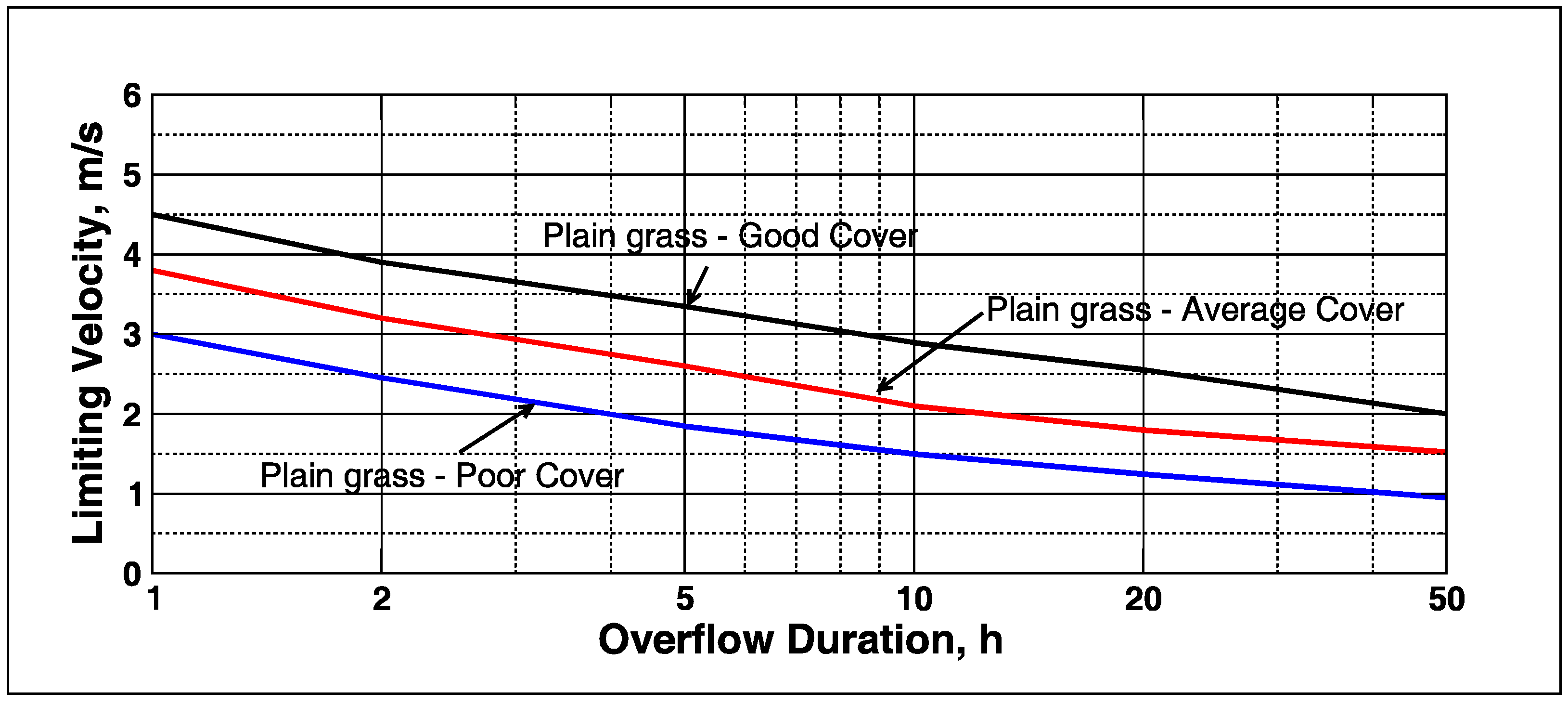
The development in this paper is based on a design nomogram for erosional stability of grass-covered slopes during steady overflow presented by Hewlett et al. [11]. This nomogram used full-scale steady overflow test data to propose stability curves for three different grass qualities and other slope protection surfaces (turf reinforcement mats and concrete block systems). Each curve presents the limiting steady overflow velocity as a function of overflow duration that results in an acceptable level of erosion without putting the grass cover at risk of failure (as defined earlier). 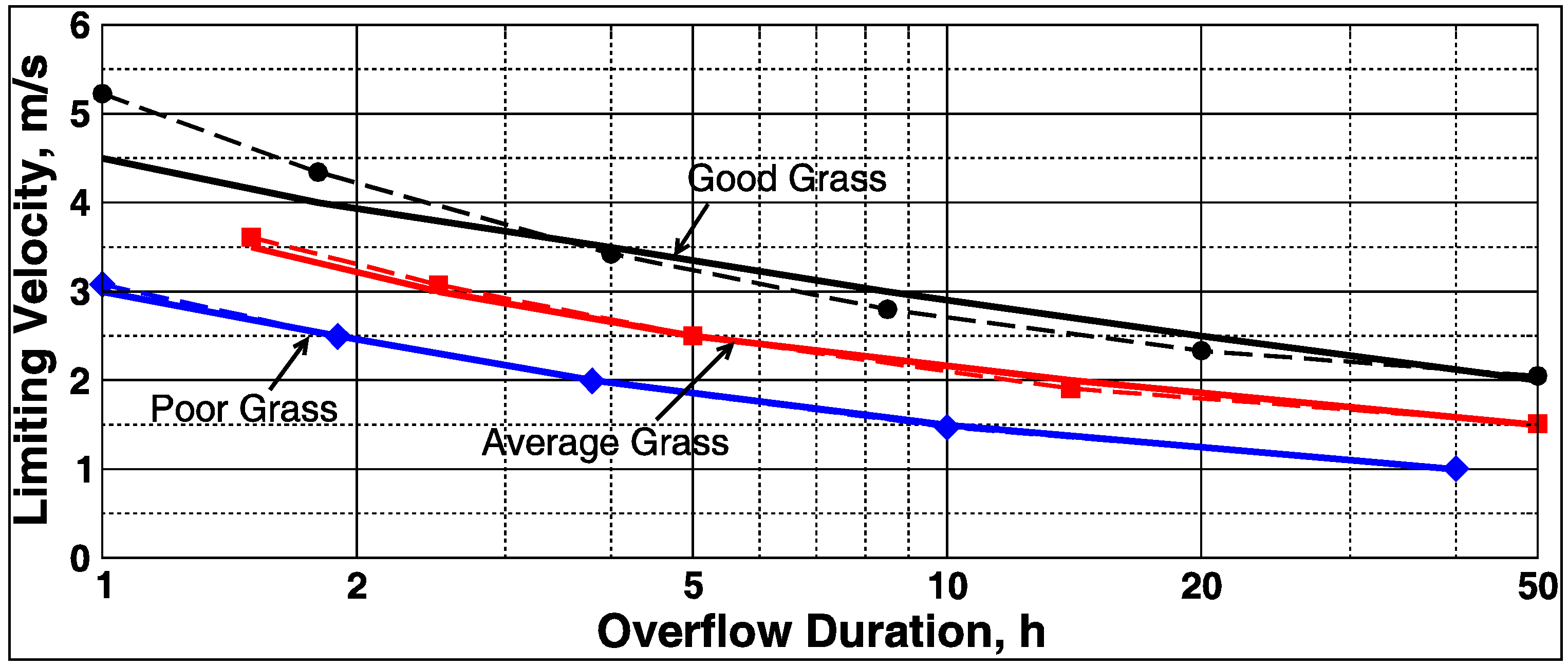Figure 1 shows a reproduction of the limiting velocity curves for grass as given in Hewlett et al. [11].

Figure 1. Limiting velocity versus overflow duration for grass (after Hewlett et al. [11]).

Figure 1. Limiting velocity versus overflow duration for grass (after Hewlett et al. [11]).

Hewlett et al. [11] had curves for good-, average-, and poor-cover plain grass as shown on Figure 1. As might be expected, the grass tolerates faster steady overflow velocities for only short durations, whereas slower velocities can be tolerated for longer durations. Hewlett et al. described the grass qualities as follows:

“Good grass cover is assumed to be a dense, tightly-knit turf established for at least two growing seasons. Poor grass cover consists of uneven tussocky grass growth with bare ground exposed or a significant proportion of non-grass weed species. Newly sown grass is likely to have poor cover for much of the first season”.

(Hewlett et al. [11])

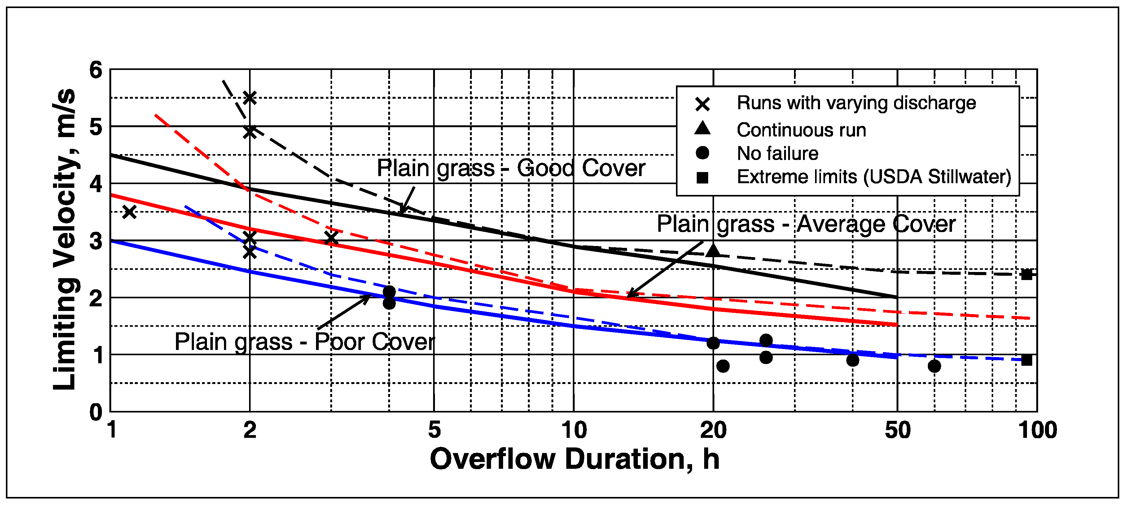
Presumably, average grass cover is something in between good and poor cover. The Hewlett et al. curves are based on earlier work by Whitehead et al. [12]. Figure 2, based on the figure in the Whitehead et al. report, includes the sparse data points on which the curves in the Whitehead et al. and the Hewlett et al. reports are based. The three design curves proposed by Whitehead et al. are shown as dashed lines, whereas the three grass curves presented by Hewlett et al. are shown by heavy solid lines. It is interesting to note that the Hewlett et al. curves for grass were adjusted downward on the low-duration side of the plots in comparison to the curves and data given by Whitehead et al. There was no explanation for this adjustment, but the result is that the Hewlett et al. curves become more conservative on the low-duration end when compared to the guidance given by Whitehead et al.

Figure 2. Erosion resistance of grass-lined spillways (after Whitehead et al. [12]).

Figure 2. Erosion resistance of grass-lined spillways (after Whitehead et al. [12]).

For unchanging steady overflow the Hewlett et al. curves can be interpreted as duration limits for tolerable overflow velocities resulting from discharge flowing over a slope having some flow resistance due to grass. Every point on a curve represents an equivalent cumulative flow condition, i.e.,

$$[u_1,T_1] \text{is} \text{erosionally} \text{equivalent} \text{to} [u_2,T_2]$$

(1)

where u is the limiting velocity and T is the flow duration at the point where the limiting velocity intersects the curve for a specific quality of grass. Erosional equivalence means that any combination of u,T that intersects a curve will result in the same erosional damage (defined as the tolerable limit for that grass quality) as any other combination of u, T that intersects the same curve at a different location. If a combination of u,T goes above the designated curve, grass failure will occur. Likewise, if a combination of u, T is below the curve, the grass will withstand the overflow. Note: the expression given in Equation (1) is not a mathematical equation; but instead it is a statement of erosional equivalence. As an example for good grass, a limiting velocity of u₁ = 3 m/s lasting for a duration of T₁ = 8 h is considered equivalent to a limiting velocity of u₂ = 2 m/s lasting for a duration of about T₂ = 50 h as seen in Figure 1 or Figure 2 because both of these combinations fall on the good grass curve.

Dean et al. [13] used numerical values manually extracted from the Hewlett et al. grass-cover curves (Figure 1) to examine the underlying physical mechanism that might be responsible for the form of the tolerable velocity limit curves. They assumed that cumulative tolerable erosion, E, took the form:

$$E_m=K_m\left(u^m-u_c^m\right)t\hspace{1em}\hspace{1em}\hspace{1em}foru>u_c$$

(2)

where K_m is a proportionality constant, u_c is a critical threshold erosion velocity, and t is time. Three possibilities were investigated: (a) flow velocity above a certain threshold velocity given when the exponent m = 1; (b) shear stress [τ_o proportional to u²] above a certain threshold shear stress when m = 2; and (c) stream power [P_s = (τ_o u) proportional to u³] above a certain threshold stream power when m = 3. (Note that Hanson and Temple [8] assumed an erosion rate based on excess shear stress.)

Dean et al. [13] performed least-squares best-fits of Equation (2) to the Hewlett et al. curves for grass covers using the three values of exponent m. Appropriate best-fit values were determined for the threshold velocities (u_c) and erosion limits (E_m/K_m) so that the error of the curve-fit was minimized. The analysis showed that the assumption of excess stream power (m = 3) had the smallest standard error by a significant margin when the three equations were fitted to all three grass quality curves. This yielded the following equation for the tolerable grass design curves:

$$\left(u^3-u_c^3\right)t=\frac{E_3}{K_3}=G_F\text{\hspace{1em}\hspace{1em}for\hspace{0.17em}\hspace{0.17em}}u>u_c$$

(3)

with the best-fit values shown in Table 1.

Table 1. Results for the best-fit of Equation (3) to the Hewlett et al. [12] grass curves.

Grass Quality	Threshold Velocity uc (m/s)	Erosion Limit E3/K3 = GF (m3/s2)	Std. Error in Velocity (m/s)
Good Cover	1.80	0.492 × 106	0.38
Average Cover	1.30	0.229 × 106	0.12
Poor Cover	0.76	0.103 × 106	0.04

Table 1. Results for the best-fit of Equation (3) to the Hewlett et al. [12] grass curves.

Grass Quality	Threshold Velocity uc (m/s)	Erosion Limit E3/K3 = GF (m3/s2)	Std. Error in Velocity (m/s)
Good Cover	1.80	0.492 × 106	0.38
Average Cover	1.30	0.229 × 106	0.12
Poor Cover	0.76	0.103 × 106	0.04

Stream power is the time rate of flow work per unit surface area, and the best-fit analysis of Equation (2) led Dean et al. to conclude that cumulative work (W = P_s·t) done on the slope by the flowing water, in excess of some critical value of work, was the physical mechanism responsible for the trends given in the Hewlett et al. [12] limiting velocity versus duration curves. Figure 3 shows the best-fit obtained by Dean et al. compared to the original Hewlett et al. curves for three types of grass. The heavy solid lines are the Hewlett et al. curves, and the symbols connected by lighter dashed lines are the best-fit values. Note the very good fits for average and poor grass (also indicated by the standard deviations in Table 1).

Figure 3. Dean et al. (2010) [13] best fit of Equation (3) to Hewlett et al. (1987) [11] curves.

Figure 3. Dean et al. (2010) [13] best fit of Equation (3) to Hewlett et al. (1987) [11] curves.

The most deviation between velocities predicted using the best fit of Equation (3) and the original Hewlett velocities occurred at the short durations, and this is seen in Figure 3 for good grass at short durations. Given that the Hewlett curves have lower velocities at short-durations when compared to the Whitehead et al. curves (see Figure 2), this over-prediction by the best-fit procedure for good grass at short durations should not be too much of a concern. Note there could be additional “almost” best-fits of the two-parameter equation that might result in different values for the threshold velocity and the erosion limit.

The formulation based on cumulative excess work might imply that the grass surface is fairly homogeneous in structure and strength. If this were the case, then we should expect erosion to be somewhat uniform, and grass damage would occur nearly simultaneously over the entire region subjected to the same flow conditions. Of course, this is not realistic, and erosion will occur sporadically at isolated “hot spots” or weaknesses in the grass cover. The implicit assumption of Dean et al. cumulative excess work model is that the model gives an indication when the isolated grass cover damage begins to become locally problematic as determined by analysis of the original full-scale test data that resulted in the Hewlett et al. curves.

3. Slowly-Varying Overflow on Grass Slopes

Many overflow situations are characterized by relatively slow variations in the overflow water depth that occur over durations of hours or days. For example, river levels can rise to a peak level and then fall again with passage of the flood wave downstream, and this causes a corresponding variation of the overflow velocity on the grass-covered slope. Likewise, storm surges propagating into estuarine systems can cause overflow variations at protective levees lasting for many hours. Rainwater run-off can cause reservoirs to overflow with similar overtopping hydrographs. 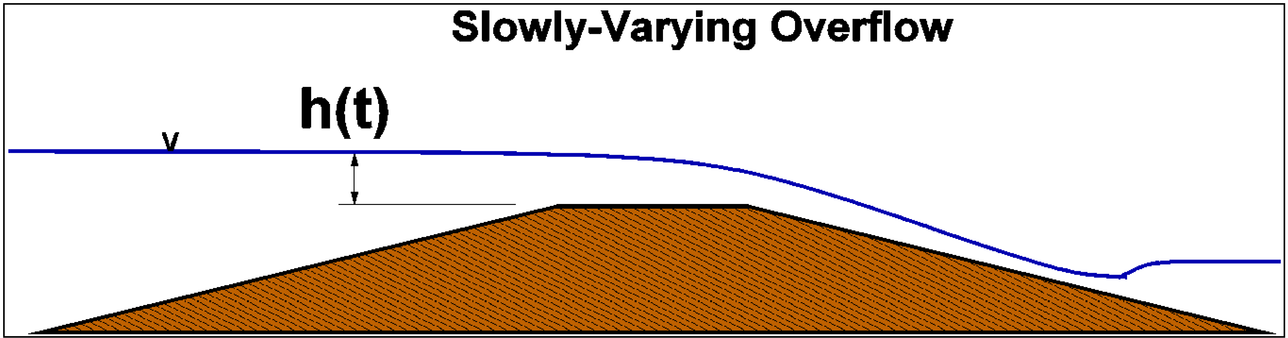Figure 4 illustrates a water level above the structure crest that slowly varies in time.

Figure 4. Slowly-varying overflow of a levee.

Figure 4. Slowly-varying overflow of a levee.

The following developments discount any influence of wave action that might accompany the coastal storm surge. Therefore, wave overtopping combined with storm surge overflow occurring at sea dikes situated at the coastline would not be a valid application of the methodology developed below because storm surge is typically accompanied by large waves. However, as storm surges propagate into estuaries, embankment or levee overtopping can occur where wave action may be limited by narrow fetches or the wave-generating wind may have abated by the time storm surge affects upper portions of the estuary. These situations would be a more appropriate application of the methodology. Future work will include the cases of tolerable time-varying overtopping due to waves only and to combined wave and surge overtopping by using erosional equivalence concepts with individual overtopping waves.

The tolerable erosion limit criterion given by Equation (3) is based on a constant limiting velocity over a given duration; but if cumulative excess flow work is responsible for eventual instability of grass slopes, there is no reason that velocity cannot vary slowly in time as the water level above the crest changes. Therefore, the criterion for tolerable cumulative excess work below the erosional limit for grass (G_F) can be given as the integral between t = 0 and t = T as

$${\displaystyle \underset{0}{\overset{T}{\int }}\left(\hspace{0.17em}{[u(t)]}^3-u_c^3\right)}\hspace{0.17em}dt\le G_F\text{\hspace{1em}\hspace{1em}for\hspace{0.17em}\hspace{0.17em}}u>u_c$$

(4)

where T is the duration of the overflow event. Dean et al. [13] noted that the limiting velocity, u, can be expressed in terms of overflow discharge under the conservative assumption that the flow velocity on the grass slope had reached terminal velocity, and the force balance described by the steady-flow resistance equation was piece-wise applicable to slowly-varying overflow. They used the Darcy-Weisbach steady-flow resistance equation at terminal velocity that is essentially the same as the Chezy equation with the Chezy coefficient represented by a friction factor, i.e.,

$$u^3=\left(\frac{8g}{f_D}\text{sin}\theta \right)\hspace{0.17em}q\hspace{0.17em}=\hspace{0.17em}\left(\frac{2g}{f_F}\text{sin}\theta \right)\hspace{0.17em}q$$

(5)

where q is volumetric discharge per unit length of levee or embankment, θ is the landward-side levee or embankment slope angle, g is gravitational acceleration, f_D is the Darcy-Weisbach friction factor, and f_F is the Fanning friction factor. The two friction factors are related by the expression f_D = 4 f_F. The Fanning friction factor is more commonly used by chemical engineers, and it routinely appears in the European wave overtopping literature. Care must be taken not to confuse the two friction factors because often the identifying subscripts are omitted.

Substituting Equation (5) into Equation (4) and rearranging yields the integral cumulative discharge criterion for slowly-varying steady overflow:

$$V_{ET}(t)={\displaystyle \underset{0}{\overset{T}{\int }}\left[q(t)-q_c\right]}\hspace{0.17em}dt\le G_F\hspace{0.17em}\left(\frac{f_F}{2g\hspace{0.17em}\text{sin}\theta }\right)\text{\hspace{1em}\hspace{1em}for\hspace{0.17em}\hspace{0.17em}}q>q_c$$

(6)

where the critical discharge is given by:

$$q_c=\left(\frac{f_F}{2g\hspace{0.17em}\text{sin}\theta }\hspace{0.17em}\right)\hspace{0.17em}{u}_c^3$$

(7)

and the parameter V_ET(t) is used to designate the integration in Equation (6). A discrete version of the integral Equation (6) can be written as:

$$V_{ET}(t)={\displaystyle \sum _{n=1}^N\left(q_n-q_c\right)}\hspace{0.17em}\mathrm{\Delta }{t}_n\le G_F\hspace{0.17em}\left(\frac{f_F}{2g\hspace{0.17em}\text{sin}\theta }\right)\text{\hspace{1em}\hspace{1em}\hspace{1em}for\hspace{0.17em}\hspace{0.17em}}{q}_n>q_c$$

(8)

In Equation (8), the subscript n refers to a discrete value of overflow discharge, N is the total number of discrete discharges, and ∆t_n is the uniform duration associated with each discrete discharge. The total duration of overflow is T = N·∆t_n. It is interesting to note that both sides of the inequality in Equation (8) have units of m³/m, so the summation of terms on the left side of the inequality in Equation (8) represents all the overflow water volume (per unit levee or embankment length) as a function of time greater than a critical discharge volume that is given by q_c·∆t_n. The right-hand side of the inequality in Equation (8) represents the tolerable upper limit of cumulative overflow water above the critical discharge volume. Therefore, the parameter V_ET means “cumulative (or total) excess water volume” which is directly proportional to the cumulative excess work (CEW).

Application of Equation (8) to estimate tolerable cumulative overflow for grass slopes requires a discrete time-history of slowly-varying overflow discharge (q_n), estimates of the critical velocity (u_c) and the grass erosional limit (G_F), the levee or embankment slope angle (θ), and a value for the Fanning friction factor (f_F). Values of critical velocity (u_c) and grass erosional limit (G_F) associated with the Hewlett et al. [11] curves are given in Table 1. However, alternate values for more robust levee grasses can be used if such values have been determined from full-scale overflow tests.

One difficulty is specifying a suitable value for the Fanning friction factor (f_F). Friction factors appropriate for grass are implicitly included in the Hewlett et al. velocity curves, but they are not known outright. Furthermore, the friction factor can be shown to be a function of flow depth; thus, the friction factor will vary in magnitude during slowly-varying overflow. Hughes [14] analyzed likely variations of the Fanning friction factor as reported in the literature, and he concluded that the range f_F = 0.01–0.02 was a reasonable representative average for overtopped grass-covered levee slopes for overflow water levels ranging between 0.15 m and 0.6 m above the levee crest. This range is expected to encompass many overflow conditions. For practical applications a constant value of f_F = 0.015 seems appropriate for typical grass-covered slopes, but some situations may require different values for the friction factor.

4. Idealized Representation of Slowly-Varying Overwash Discharge

In the absence of measured or predicted overflow water depth hydrographs (i.e., storm surge or flood hydrographs), an approximation can be made that mimics the time-varying overflow process. An idealized representation of slowly-varying overflow discharge should start with zero discharge when the water level reaches the levee or embankment crest elevation, increase monotonically over time to a maximum discharge when the water elevation is at its greatest elevation above the crest, and then decrease monotonically back to zero discharge. Whereas, a simple straight-line approximation for the increase and decrease of overflow water level could be used as a first approximation, it is better to have a more realistic continuous function without any singularities or discontinuities.

Several mathematical formulas are available that could be adapted for approximating time-varying overflow discharge. Cialone et al. [15] developed a synthetic symmetrical storm surge hydrograph in which the rising and falling portions of the hydrograph were represented by an exponential decay. Their synthetic hydrograph was given as the following:

$$S(t)=S_p\left(1-e^{-\left|D/\left(t-t_0\right)\right|}\right)\hspace{0.17em}$$

(9)

where S(t) is the time-dependent surge, S_p is the peak surge, D = half the storm surge duration, t = time, and t₀ is the time of peak surge.

Measurements indicated that the falling limbs of storm surges are steeper than the rising limbs, and this led Zevenbergen et al. [16] to represent the falling limb of the storm surge by adding a dimensionally nonhomogeneous term to the equation of Cialone et al. This resulted in the synthetic hydrograph being described by two equations:

$$\begin{array}{l}S(t)=S_p\left(1-e^{-\left|D/\left(t-t_0\right)\right|}\right)\text{ for }t<t_o\\ S(t)=S_p\left(1-e^{-\left|D/\left(t-t_0\right)\right|}\right)-0.14\hspace{0.17em}\left(t-t_o\right)\hspace{0.17em}{\text{e}}^{\text{-0.18}\left({\text{t-t}}_{\mathrm{o}}\right)}\text{ for }t>t_o\end{array}$$

(10)

More recently, Xu and Huang [17] proposed equations that successfully represented Gulf of Mexico storm surges when the empirical coefficients were determined from data. There equations were given as:

$$\begin{array}{l}S(t)=S_p\left(1-a\cdot e^{-\left|b/\left(t-t_0\right)\right|}\right)\text{ for }t<t_o\\ S(t)=S_p\left(1-c\cdot e^{-\left|d/\left(t-t_0\right)\right|}\right)\text{ for }t>t_o\end{array}$$

(11)

where a, b, c, and d are dimensionless empirical coefficients. Fitting of Equation (11) to measured Gulf of Mexico category 4 and 5 hurricane storm surge hydrographs resulted in values for the four coefficients shown in Table 2.

Table 2. Empirical coefficients for Xu and Huang [17] synthetic storm surge hydrograph.

Hurricane	a	b	c	d
Category 3	1	3	0.9	4
Category 4	1	4	1.2	5

Table 2. Empirical coefficients for Xu and Huang [17] synthetic storm surge hydrograph.

Hurricane	a	b	c	d
Category 3	1	3	0.9	4
Category 4	1	4	1.2	5

Of course, storm surges may not be good representations of the time-varying water elevations associated with flooding events that cause steady overflow (without wave action).

In this paper we propose an alternative hypothetical hydrograph to represent time-varying overflow of a levee or embankment. For convenience, we selected the well-known symmetric formula for the normal (or Gaussian) probability density function. However, in this application we are not using the formula for estimating probability; instead we are just applying a mathematical form that provides properties that are similar to an actual overflow hydrograph.

The equation for a normal probability distribution is:

$$p(x)=\frac{1}{\sigma \sqrt{2\pi }}\hspace{0.17em}\text{exp}\hspace{0.17em}\left[-\frac{{\left(x-\mu \right)}^2}{2{\sigma }^2}\right]$$

(12)

where p is the probability associated with x, μ is the mean value of x, and σ is the standard derivation of the probability density function. The probability density function is symmetric about the mean, the maximum of the density function occurs at the mean, and the area beneath the curve given by Equation (12) is equal to unity.

Adopting Equation (12) for use in describing the time-varying overwash water level is accomplished by the following substitutions:

• Let x equal time, t_s, in seconds. This means that standard deviation, σ, will also have units of seconds.
• Let probability p(x) equal instantaneous overwash water level, h(t_s) as a function of time, as illustrated in Figure 4.
• One feature of Equation (12) is that 99.6% of the area under the curve is contained by three standard deviations on each side of the peak that occurs at x = μ. Therefore, let 6σ ≈ T_s = total duration of overflow in seconds, and substitute σ = T_s/6. Also, let the mean value μ = T_s/2. This results in overflow beginning very close to t_s = 0, and ending very close to t_s = T_s. Maximum overflow water depth and discharge occur at time t_s = T_s/2.
• Add a scaling factor, C_A, to Equation (12) that represents the total area under the curve.

Making these substitutions into Equation (12) gives the following equation for the time-varying distribution of overwash elevation.

$$h(t_s)=\frac{6\hspace{0.17em}{C}_A}{\sqrt{2\pi }\hspace{0.17em}{T}_s}\hspace{0.17em}\text{exp}\hspace{0.17em}\left[\frac{-18\hspace{0.17em}{\left(t_s-\frac{T_s}{2}\right)}^2}{T_s^2}\right]$$

(13)

The peak overflow water depth (h_p) occurs at t_s = T_s/2, and from Equation (13) the scaling factor equals:

$$C_A=\frac{\sqrt{2\pi }\hspace{0.17em}{T}_s\hspace{0.17em}{h}_p\hspace{0.17em}}{6}\hspace{0.17em}$$

(14)

Substituting Equation (14) into Equation (13) gives the idealized hydrograph of overflow water depth in terms of the overflow duration and the peak water depth above the structure crest, i.e.,

$$h(t_s)=h_p\hspace{0.17em}\text{exp}\hspace{0.17em}\left[\frac{-18\hspace{0.17em}{\left(t_s-\frac{T_s}{2}\right)}^2}{T_s^2}\right]$$

(15)

The corresponding slowly-varying overflow discharge hydrograph can be approximated by substituting Equation (15) into the broad-crested weir formula (e.g., Henderson [18])

$$q(t_s)={\left(\frac{2}{3}\right)}^{3/2}\sqrt{g}\hspace{0.17em}{\left[h(t_s)\right]}^{\hspace{0.17em}3/2}$$

(16)

where q is overflow discharge per unit crest width, and g is gravitational acceleration. This substitution gives the expression

$$q(t_s)={\left(\frac{2}{3}\right)}^{3/2}\sqrt{g}\hspace{0.17em}{(h_p)}^{3/2}\hspace{0.17em}\text{exp}\hspace{0.17em}\left[\frac{-27\hspace{0.17em}{\left(t_s-\frac{T_s}{2}\right)}^2}{T_s^2}\right]$$

(17)

Equation (17) can also be expressed in terms of the peak discharge (q_p) as:

$$q(t_s)=\hspace{0.17em}{q}_p\hspace{0.17em}\text{exp}\hspace{0.17em}\left[\frac{-27\hspace{0.17em}{\left(t_s-\frac{T_s}{2}\right)}^2}{T_s^2}\right]$$

(18)

where:

$$q_p={\left(\frac{2}{3}\right)}^{3/2}\sqrt{g}{\left(h_p\right)}^{\hspace{0.17em}3/2}$$

(19)

Finally, the cumulative overflow water volume per unit crest width as a function of time is found by integrating Equation (18), i.e.,

$$V_W(t_s)={\displaystyle \underset{-\infty }{\overset{t_s}{\int }}q(t_s)\hspace{0.17em}dt}=\hspace{0.17em}{q}_p\hspace{0.17em}{\displaystyle \underset{-\infty }{\overset{t_s}{\int }}\text{exp}\hspace{0.17em}\left[\frac{-27\hspace{0.17em}{\left(t_s-\frac{T_s}{2}\right)}^2}{T_s^2}\right]\hspace{0.17em}dt}$$

(20)

or

$$V_W(t_s)=\sqrt{\frac{\pi }{3}}\frac{q_p\hspace{0.17em}{t}_s\hspace{0.17em}}{6}\hspace{0.17em}\left\{1+\text{erf\hspace{0.17em}}\left[\frac{3\sqrt{3}}{T_s}\left(t_s-\frac{T_s}{2}\right)\right]\right\}$$

(21)

where erf is the mathematical error function. The total cumulative overflow water volume per unit embankment width is given to a close degree of approximation when t_s = T_s in Equation (21), i.e.,

$$V_W(T_s)={\left(V_W\right)}_{Total}=\sqrt{\frac{\pi }{3}}\frac{q_p\hspace{0.17em}{T}_s\hspace{0.17em}}{3}\hspace{0.17em}$$

(22)

In summary, idealized formulations for slowly-varying water depth above the embankment crest (Equation 15) and overflow discharge (Equation 18) have been proposed in terms of time, the peak water depth expected during the flood event (h_p), and the duration of overflow (T_s). The water depth and discharge hydrographs are symmetric about the peak values, and the equations are dimensionally homogeneous so they can be used with any consistent set of units (i.e., all numerical coefficients are dimensionless).

Figure 5 illustrates three idealized overflow hydrographs having a maximum overflow depth of 0.25 m and overflow durations of 1, 3, and 5 h, respectively. The upper plot shows the variation in time of overflow water depth; the middle plot shows discharge per unit width; and the lower plot gives the corresponding cumulative overflow water volume per unit width as a function of time. Similar theoretical equations could be developed in the same manner, and equations with more variables, such as those proposed by Xu and Huang [17] could be fit to available measured water level hydrographs. However, in the absence of measured hydrographs and more elegant mathematical forms, the suggested hypothetical hydrographs provide a simple and reasonably realistic method for approximating time-varying overflow as part of a preliminary risk analysis.

Figure 5. Idealized overflow hydrographs and cumulative overflow water volume.

Figure 5. Idealized overflow hydrographs and cumulative overflow water volume.

5. Example Estimate of Tolerable Slowly-Varying Overflow

The following is an example that uses the proposed methodology given in this paper to estimate tolerable overflow as a function of duration during an event when the water level exceeds the embankment crest. Assume:

(1)

The variation of water level above the embankment crest occurs according to Equation (15) over a duration of T_s = 5 h = 18,000 s.

(2)

The peak water level above the crest is h_p = 0.25 m.

(3)

The embankment grass is considered “good,” so the parameters for critical threshold velocity and erosional limit in Table 1 for “good grass” are appropriate if no other full-scale test results are available for the particular grass/soil combination.

(4)

The embankment landward-side slope is 1V-on-3H (θ = 18.4°).

(5)

The grass cover Fanning friction factor is approximately f_F = 0.015.

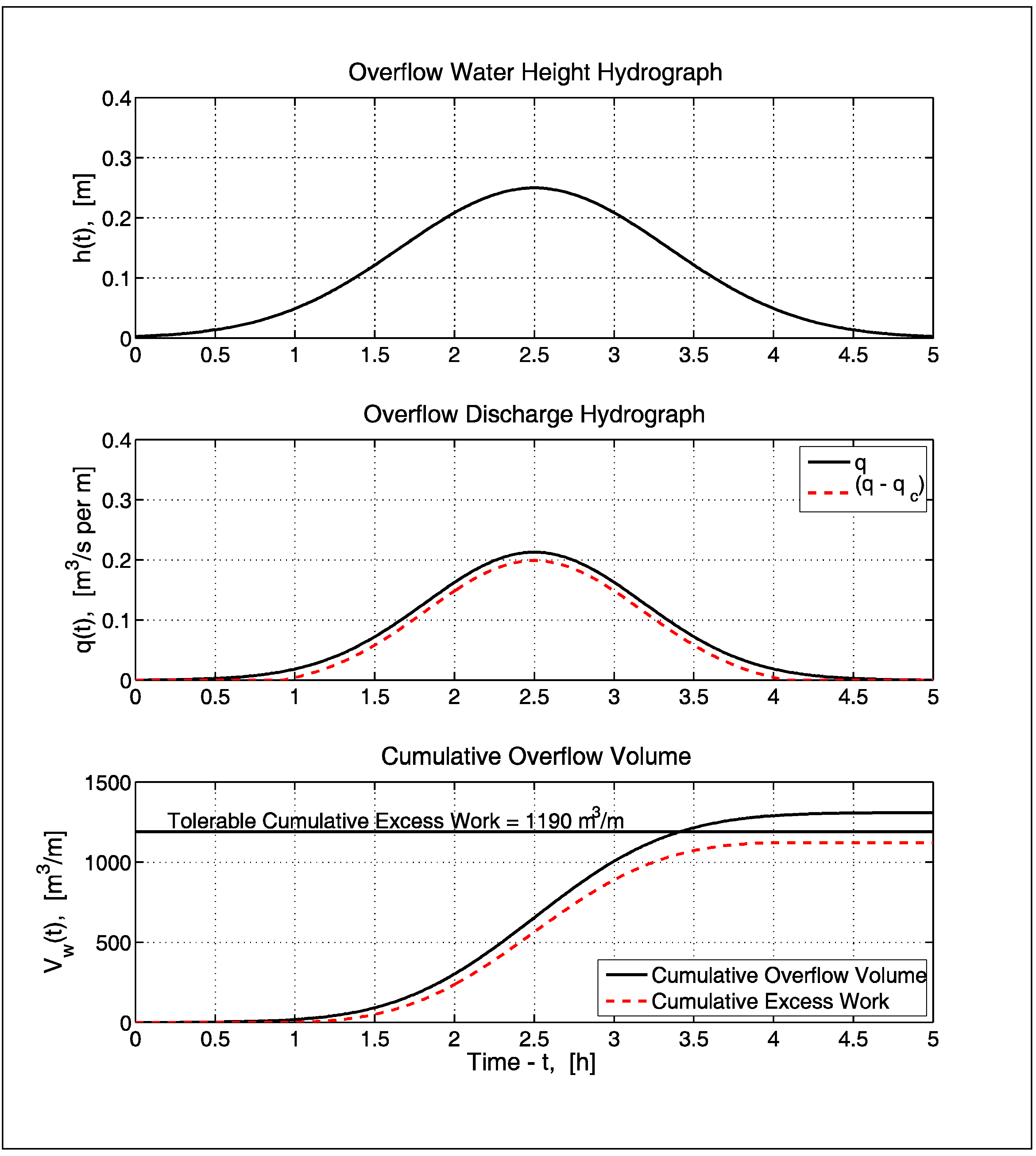
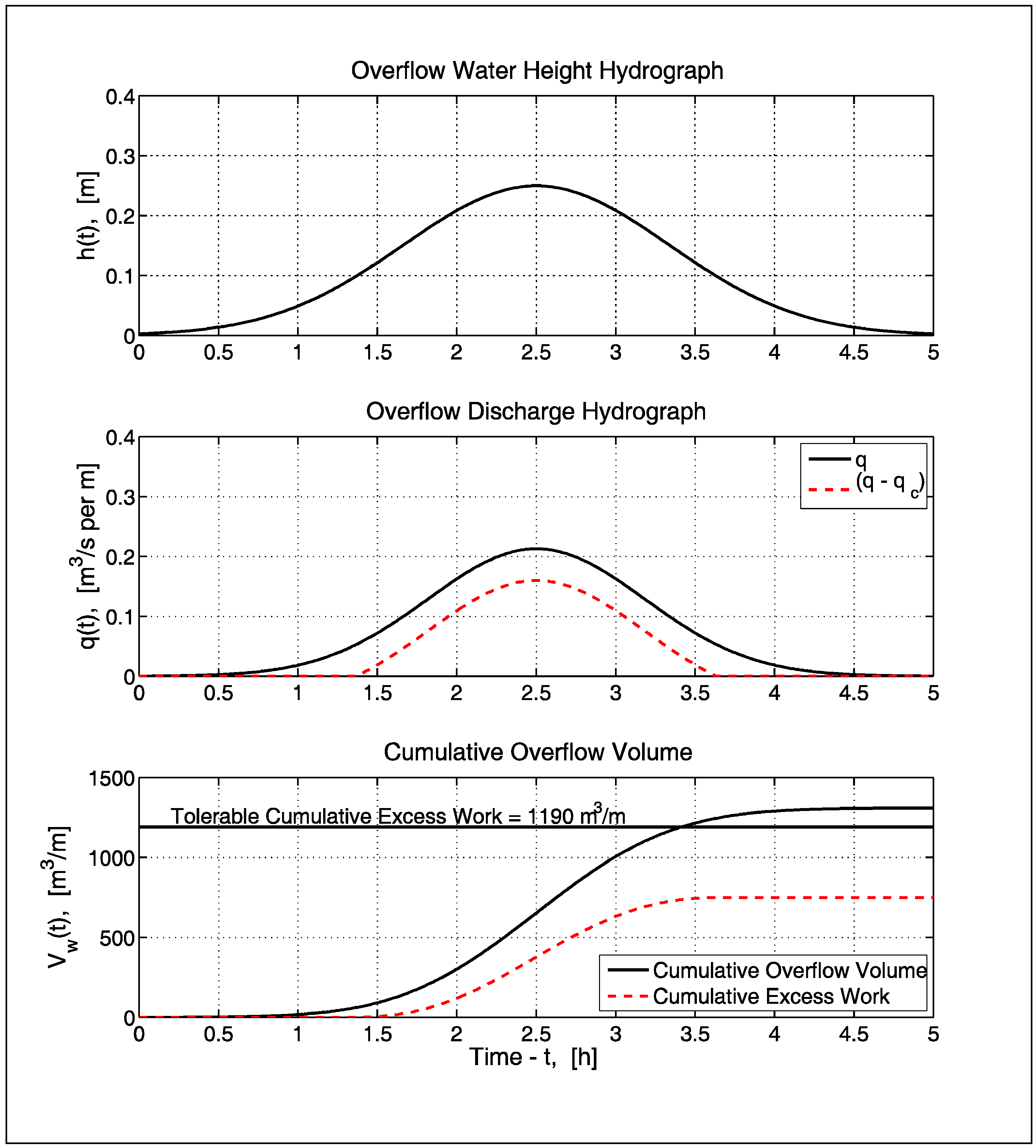
Figure 6. Example of cumulative excess work estimate for “good grass” (u_c = 1.8 m/s).

Figure 6. Example of cumulative excess work estimate for “good grass” (u_c = 1.8 m/s).

The solution is found by using Equation (18) in the discrete version of the cumulative excess work equation given by Equation (8). First, the peak discharge is determined using Equation (19), i.e.,

$$q_p={\left(\frac{2}{3}\right)}^{3/2}\sqrt{g}{\left(h_p\right)}^{\hspace{0.17em}3/2}={\left(\frac{2}{3}\right)}^{3/2}\sqrt{9.814\hspace{0.17em}{\text{m/s}}^{\text{2}}}{\left(0.25\text{\hspace{0.17em}m}\right)}^{\hspace{0.17em}3/2}=0.213\hspace{0.17em}{\text{m}}^{\text{3}}\text{/s per m}$$

(23)

and the time-varying discharge (Equation 18) becomes:

$$q_n(t_s)=\hspace{0.17em}(0.213\hspace{0.17em}{\text{m}}^{\text{3}}\text{/s per m)}\hspace{0.17em}\text{exp}\hspace{0.17em}\left[\frac{-27\hspace{0.17em}{\left(t_s-\frac{18,000\text{\hspace{0.17em}s}}{2}\right)}^2}{{\left(18,000\text{\hspace{0.17em}s}\right)}^2}\right]$$

(24)

Next, find the critical discharge associated with the critical threshold velocity (u_c = 1.8 m/s from Table 1) using Equation (7).

$$q_c=\left(\frac{f_F}{2g\hspace{0.17em}\text{sin}\theta }\hspace{0.17em}\right)\hspace{0.17em}{u}_c^3=\left(\frac{0.015}{2\left(9.814\hspace{0.17em}{\text{m/s}}^{\text{2}}\right)\hspace{0.17em}\text{sin}\left({18.4}^o\right)}\hspace{0.17em}\right)\hspace{0.17em}{\left(1.8\text{\hspace{0.17em}m/s}\right)}^{\hspace{0.17em}3}=0.014\hspace{0.17em}{\text{m}}^{\text{3}}\text{/s per m}$$

(25)

Finally, the cumulative excess work is found from Equation (8) as the summation:

$$\begin{array}{l}{V}_{ET}(t)={\displaystyle \sum _{n=1}^N\left(q_n-q_c\right)}\hspace{0.17em}\mathrm{\Delta }{t}_n\le G_F\hspace{0.17em}\left(\frac{f_F}{2g\hspace{0.17em}\text{sin}\theta }\right)\le 492,000\hspace{0.17em}{\text{m}}^{\text{3}}{\text{/s}}^{\text{2}}\hspace{0.17em}\left(\frac{0.015}{2\left(9.814\hspace{0.17em}{\text{m/s}}^{\text{2}}\right)\hspace{0.17em}\text{sin}\left({18.4}^o\right)}\hspace{0.17em}\right)\\ \text{or}\\ V_{ET}(t)={\displaystyle \sum _{n=1}^N\left(q_n-q_c\right)}\hspace{0.17em}\mathrm{\Delta }{t}_n\le 1,190\hspace{0.17em}{\text{m}}^{\text{3}}\text{/m\hspace{1em}\hspace{1em}\hspace{1em}for\hspace{0.17em}\hspace{0.17em}}{q}_n>q_c\end{array}$$

(26)

where G_F = 492,000 m³/s² was used from Table 1. Equation (26) can be solved in a spreadsheet using Equation (24) for q_n, Equation (25) for q_c, and an appropriate incremental time (say Δt_n = 0.01 h = 36 s).

Figure 7. Example of cumulative excess work estimate for grass with u_c = 2.8 m/s.

Figure 7. Example of cumulative excess work estimate for grass with u_c = 2.8 m/s.

Figure 6 presents the solution for this example plotted as a function of time (hours). The dashed line in the lower plot of Figure 6 shows the cumulative excess work remains just below the erosional limit for “good grass” suggested by Dean et al. [13]. For the peak water depth above the crest of h_p = 0.25 m, shorter overflow duration would increase the safety margin and larger durations would exceed the tolerable erosional limit.

Note in this example with a critical velocity of only 1.8 m/s (Figure 6), there is not much difference between the cumulative excess work volume (dashed line in Figure 6) and the total cumulative overflow volume (solid line). Figure 7 shows the cumulative excess work estimated for a more robust embankment grass cover having a critical velocity of u_c = 2.8 m/s. All other parameters for this example are the same as used for the results shown in Figure 6.

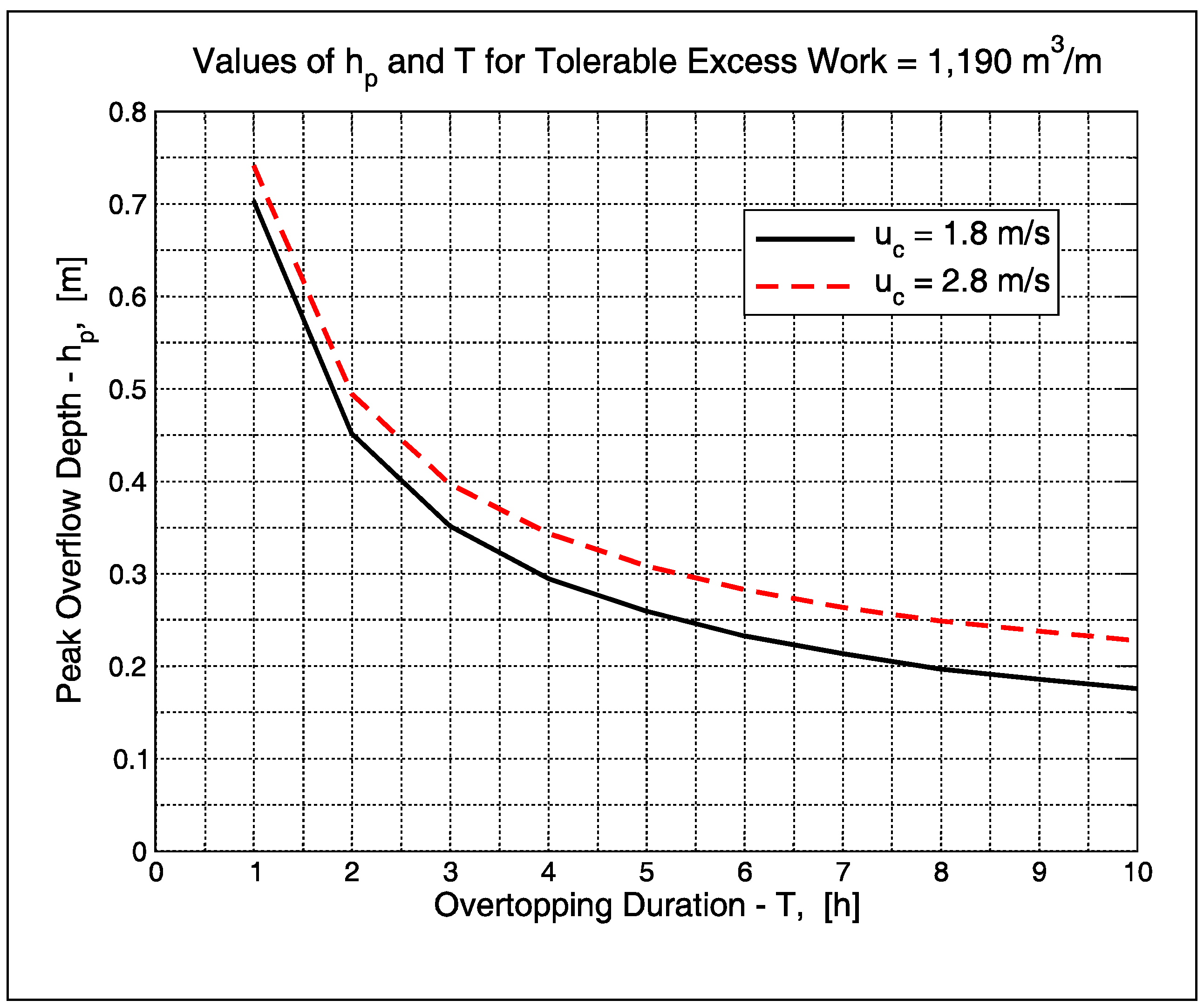
Through trial and error it is possible to determine “equivalence pairs” of peak water depth and overflow duration (h_p, T_s) that just reach the tolerable limit for overflow. However, these equivalence pairs would only apply to grass of the same quality, same critical threshold velocity, same landward-side slope, and same friction factor subjected to an overflow discharge hydrograph similar to that given by Equation (18). The plotted lines in Figure 8 show equivalence pairs that result if the cumulative excess work is equal to the tolerable cumulative excess work of 1190 m³/m. Iterative calculations were performed in which the duration was set to an integer hour, and the peak overflow depth was changed until the target cumulative excess work value was reach. All other parameters remained as given in this example. The two curves represent different values of the critical threshold velocity. Diagrams, such as those shown in Figure 8, can be used in risk analyses to assess the likelihood of grass failure associated with different projected flooding events. The estimated joint probabilities of peak surge and overtopping duration, as obtained from Monte Carlo storm surge simulations, could be used to assess whether or not the tolerable overflow limit has been surpassed. Bear in mind that grass failure is just the first step in dike or embankment failure, but a conservative criterion for tolerable overtopping would be no grass failure.

Figure 8. Equivalence pairs of peak overflow depth and overtopping duration that produce tolerable cumulative excess work of V_ET = 1190 m³/m.

Figure 8. Equivalence pairs of peak overflow depth and overtopping duration that produce tolerable cumulative excess work of V_ET = 1190 m³/m.

6. Summary and Conclusions

Engineers require estimates of tolerable overtopping limits for grass-covered levees, dikes, and embankments that might experience overflow due to storm surges or flooding. Realistic estimates can be used in both resilient design and in risk assessment. Hewlett et al. [12] presented design curves for grass-covered slopes in the form of steady overflow limiting velocity versus overflow duration. The curves were based on earlier full-scale overflow tests. The design curves were provided for three descriptions of grass cover (good, average, and poor), and these curves are used frequently for evaluation of steady overflow conditions on grass slopes. Dean et al. [13] analyzed the Hewlett et al. curves to determine the physical mechanism most likely to explain the curve shape. They concluded that flow work above a threshold velocity cubed (referred to as cumulative excess work) provided the best explanation. In this paper the concept of cumulative excess work for overflow on grass slopes is expressed in terms of slowly-varying overflow discharge (Equation 8) typical of realistic situations where the water level hydrograph above the structure crest increases to a maximum and then recedes similar to storm surges in estuaries and the passing of a flood wave in a river.

Whereas the cumulative excess work concept could be applied for any specified discharge hydrograph, this information may not be available for preliminary analyses. Hypothetical, but somewhat realistic, forms for the water level hydrograph above the embankment crest (Equation (15)) and the corresponding overflow discharge (Equations (17) or (18)) are given in terms of the values at maximum overflow (h_p or q_p) during the event and the total duration of overflow (T_s). An example application is given to illustrate use of the equations.

In the absence of additional grass and soil performance information, the values of critical threshold velocity, u_c, and the erosional limit, G_F, based on the Hewlett et al. [12] curves (given in Table 1) can be used. However, well-maintained grass with dense root systems can withstand greater cumulative overflow than the limits suggested by the Hewlett curves. Design of critical grass-protected structures should consider conducting full-scale overflow tests to establish reliable values for critical threshold velocity and tolerable cumulative excess work. Such testing could result in significant cost savings and decreased risk uncertainty.