Impacts of Agro-Ecological Practices on Soil Losses and Cash Crop Yield


1
Council for Agricultural Research and Economics—Research Centre for Agriculture and Environment, CREA-AA, 70125 Bari, Italy
2
Council for Agricultural Research and Economics—Research Centre for Vegetable and Ornamental Crops, CREA-OF, 63077 Monsampolo del Tronto (AP), Italy
*
Author to whom correspondence should be addressed.
Agriculture 2017, 7(12), 103; https://doi.org/10.3390/agriculture7120103
Submission received: 19 October 2017
/
Revised: 21 November 2017
/
Accepted: 11 December 2017
/
Published: 15 December 2017
(This article belongs to the Special Issue Sustainable Crop Production Intensification)
Abstract
:The aim of this study was to determine the impact of agro-ecological practices on soil losses, by assessing experimental field topography changes and cauliflower crop yield after an artificial extreme rainfall event. Data were collected in an innovative experimental device in which different combined agronomic strategies were tested such as hydraulic arrangement, crop rotations and agro-ecological service crops (ASC) introduction. The collection of elevation data was carried out in kinematic way before rainfall, and in punctual surveys to evaluate the effects of artificial event on this parameter. Non-parametric tests were performed to evaluate differences between samples. High-resolution digital elevation models were generated from independent data using kriging, and elevation difference maps were produced. The results indicated that the data before and after the artificial rainfall were statistically different. The raised strips suffered soil loss showing that the strip with permanent intercropping was higher than that in the absence of ASC. A significant rise of elevation was registered in the furrowed strips after rainfall, and deposition of soil occurred at the lowest areas of the experimental field. Moreover, the study showed a relationship between cash crop yield and elevation: the areas with lower elevation (higher flooding) were characterized by the lowest yield.
1. Introduction
In many agro-environments of the developed countries, due to uniformity in crop monoculture systems along with indiscriminate use of agro-chemicals, negative outcomes and vulnerabilities (e.g., wide-spread degradation of land, water and ecosystems; high GHG emissions; biodiversity losses) are becoming crucial issues [1]. These adverse environmental externalities worsen in the climate change context, particularly in Mediterranean environment. As a result of extreme rainfall events, temporary flooding of the soil, determining poor soil aeration, affects plant growth [2]. These frequent high-intensity rainfall events, which usually occur after a very dry summer, and the climatic fluctuation in short- and long-term (especially in rainfall quantity), have been pointed out as the main climatic characteristics affecting the vulnerability of the Mediterranean basin to erosion [3,4]. In particular, specialized input-intensive farming systems entail high risks of runoff and soil erosion, thus reducing the productivity of agricultural ecosystems [5].
The Food and Agriculture Organization (FAO) highlighted the great potential of diversified agro-ecological systems to reverse soil degradation, restore degraded land and rebuild soil fertility, according to sustainable agriculture principles [6]. Indeed, sustainable agriculture is based on different agronomic practices that meet current and future society needs for food and feed, ecosystem services and human health, maximizing the net benefit for people [7]. Keeping or improving the organic carbon content in the soil and the related soil fertility properties can be achieved with conservation soil tillage systems, which leave more crop residues on the surface because the soils are not turned over, and by using organic fertilizers and amendments [8,9]. Soil organic matter is of greatest importance for agricultural systems adaptation, since it increases water infiltration and surface soil aggregation, thus diminishing soil losses through runoff [10]. In addition, in-field species diversity often plays a key role in delivering resilience, acting as a buffer against environmental and economic risks, and enabling adaptation to changing climate and land use conditions [11]. The diversification of farming systems, based on the rotation and association of cash crops and the introduction of complementary, break crops or living mulches (LM), can fulfill the need of producing food, feed and fiber [12]. In particular, the inclusion of cover crops in a rotation provides soil cover and helps regulate microclimate and local hydrological processes, thus preventing soil erosion by wind and rainwater strength during extreme rainfall events, which reduce organic matter content in the long run. In crop rotations, LM, planted either before or concurrent with a main crop and maintained as a living ground cover throughout the growth cycle, may provide many beneficial ecosystem services (e.g., prevent nitrate leaching, improve soil physical characteristics; contribute to reducing surface water runoff, etc.); thus, cover crops can be defined as “agro-ecological service crops”—ASC [13].
On the other hand, break crop utilization limits nutrient leaching, scavenging the soil residual N and making it available for subsequent cash crops, and leguminous green manures can fix large quantities of atmospheric N2 [10]. However, these crops should be opportunely managed and farmers’ perception should be taken into account [14]. In Mediterranean regions of Europe, the conservation no-till or minimum tillage systems based on the use of a roller crimper to terminate cover crops could have great potential to provide ecosystem services (i.e., soil temperature control, energy and water saving, weed control) in organically managed vegetable cropping systems [15].
All of the above-described agro-ecological techniques can be tested as potential strategies for organic horticulture adaptation to climate change.
Moreover, topography and landform are among the most obvious relevant causes of crops yield variation because of their direct effect on micro-climate and their water-related soil factors [16,17]. Accurate representation of field topography in the form of digital elevation models (DEMs) is required to implement management for more efficient production systems. For example, DEMs can be used to identify runoff-contributing areas and calculate slopes for use in field-runoff and filtration models [18] or for soil erosion [19,20]. Modern mapping technologies such as real-time kinematic differential GPS (DGPS), with higher accuracy of topographic measurements (centimeter level position accuracy), offer a new approach to the monitoring of this dynamic environment and to evaluate the changes in elevation surfaces [21].
As better described in Diacono et al. [22], in the MITIORG long-term experimental device (southern Italy), soil surface shaping as a kind of ridge system was carried out to increase rooting depth layer, allowing crop survival in the event of flooding, and to facilitate the lateral outflow of excess water. This technique was combined with organic fertilizer and amendment application, which can increase the soil’s water retention capacity and infiltration, and farming system diversification.
An approach that integrates conservation agriculture and sustainable crop production intensification can be considered a win-win solution in the case of income reduction due to climate change effects. Therefore, more cash crops have been cultivated in rotation on flat soil strips during each cropping season.
The main goal of this study was to evaluate the influence of different agro-ecological practices on soil erosion by water, by assessing field topographic features with a very high-resolution DEM, before and after an artificial extreme rainfall event, and cash crop yield after the same event. The ultimate goal of the ongoing research is to suggest agro-ecological technique combinations for the potential adaptation of horticultural systems to climate change.
2. Materials and Methods
2.1. Study Site and Experimental Device
The study was carried out in the innovative MITIORG organic long-term field experiment (Long-term climatic change adaptation in organic farming: synergistic combination of hydraulic arrangement, crop rotations, agro-ecological service crops and agronomic techniques), on the research farm ‘Azienda Sperimentale Metaponto’ of the Council for Agricultural Research and Economics, Research Centre for Agriculture and Environment (CREA-AA) (lat. 40°24′ N; long. 16°48′ E).
The soil is classified as a Typic Epiaquert [23] and it is poorly drained, consisting mostly of swelling clays, and the clay (about 60%) and silt (30%) contents increase with depth. An average value of 1.23 (g cm−3) for bulk density was considered in order to have an indicator of soil compaction.
The climate is classified as “accentuated thermomediterranean” according to the UNESCO-FAO soil classification system [24], with mean monthly temperatures of 8.8 °C in the winter and 24.4 °C in the summer. The site is generally characterized by winter temperatures which can fall below 0 °C, and summer temperatures which can rise above 40 °C.
Mean monthly minimum and maximum temperature and total rainfall were recorded at the agro-meteorological station of the experimental farm. Due to the absence of extreme rainfall events (which are not completely predictable) during the field trial, in a previous study it was not possible to verify the effects on climate change adaptation of the combined agro-ecological practices [22]. Therefore, it was decided to artificially produce a heavy rainfall event by flooding the field. This artificial rainfall event was accomplished by flooding the field with about 370 mm ha−1 of water over two days, in December 2016. In particular, a two-day constant irrigation on the entire experimental field was provided by sprinkler irrigation, by applying a uniform amount of water. Due to the peculiar characteristics of the soil (high amount of clay and silt) the water started to remain on the soil surface soon after the first day of irrigation.
The field experiment was designed based on the experience learnt from previous studies on agro-ecological strategies [25]. The experimental device combines a suite of functionally integrated techniques (conceptually identified as “layers”), namely: (i) soil surface shaping; (ii) crop rotations; (iii) ASC introduction; (iv) ASC termination techniques; and (v) organic fertilization.
The base layer is the soil hydraulic arrangement by means of soil surface shaping as a kind of ridge system, in which vegetable crops are cultivated both above the raised bed (ridges 2.5 m wide, indicated as R) and in the 2.5 m flat areas (or strips) between them (indicated as FS—Figure 1).
The system is obtained by ploughing on the left-hand side of a strip and, as the plough turns the soil over, it moves it to the right. On reaching the end of the strip, the plough is taken back down the other side, resulting in build up of the soil in the strip center. The field was characterized by a slight depression along its eastern side, which could influence soil surface runoff and elevation changes in the ridges. The soil hydraulic arrangement was conceived as a semi-permanent system, since it is done every two years to avoid ridge compaction. It is sometimes used for vegetables and fruit shrubs in the study area.
Rotation (the second conceptual layer) is designed avoiding cash crop cultivation during the winter-rainy period of the year in the FS, which can be waterlogged in the case of heavy rain and/or temporary flooding, as it has frequently occurred in the study area over the last 10 years. Moreover, in order to protect the soil from erosion and to provide N to the system via biological fixation, a next conceptual layer based on tailored introduction of ASC is implemented. On top of the R, a leguminous ASC is provided as living mulch (LM) to the winter vegetable crop and maintained as a living ground cover throughout its cycle (controlling the growth by mowing). In the flat strips, the cash crops in rotation are always summer crops, and pure ASC or mixtures of different proportions of legume and non-legume crops are cultivated (being potentially unaffected by temporary water excess) in the winter-rainy period as break crops. These break ASC are terminated by the no-till roller crimper technique or they are green manured before the transplant of cash crops. The last conceptual layer consists of an organic fertilization strategy, by using commercial and/or on-farm fertilizers and amendments allowed in organic farming by Italian legislation (e.g., anaerobic digestates and composted municipal solid organic wastes), to maintain or increase long-term soil organic matter and fertility.
2.2. Experimental Setup, Treatments and Measurements
The research was carried out during the 2016–2017 season in the entire experimental field described in Figure 1, with winter cauliflower crop (Brassica oleracea L. cv. Triunphan) cultivated on the R, with different management of the legume LM, and autumn-winter ASC in the FS. On the top of two ridges, legume ASC were intercropped with the cash crop: (i) burr medic LM (Medicago polymorpha L. var. anglona); (ii) crimson clover LM (Trifolium incarnatum L.), which were compared to (iii) no living mulch control (NMC) in the third R. These three main plots were divided, as a randomized complete block design, into three sub-plots to test the second factor corresponding to the following organic fertilizers (F), allowed in organic farming [26]: (i) local anaerobic digestate fertilizer, based on cattle slurry (AD); (ii) commercial organic-mineral fertilizer (OF), based on dried cattle manure, compared to (iii) an unfertilized control (NFC). Each LM × fertilizer plot (intersection plot) resulted in about a 60 m2 area. Within each intersection plot, three random replications were defined and, therefore, each elementary plot consisted of about a 20 m2 area. The organic materials were applied before cauliflower transplanting, at a 100 kg N ha−1 rate. The cauliflower was manually transplanted on 20 October 2016 (1 × 0.60 m; 17,000 plants ha−1) and it was harvested on 21 March 2017. Following the local practices of the farmers, the crop was rainfed, and no irrigation water was distributed after transplanting, since a sufficient amount of natural rainfall occurred in late October. At harvesting, on the tested area of about 4 m2, five randomly selected cauliflower heads were collected from each elementary plot, which consisted of about 35 plants, allowing the calculation of marketable yield production.
In the flat strips, ASC mixtures were cultivated in the winter period before cash crop transplanting: (i) MIX 1 by vetch (Vicia sativa L.) + oats (Avena byzantina L.) in two strips and (ii) MIX 2 by vetch + broad bean (Vicia faba L.) in one strip, all compared to a no-ASC control (NAC).
2.3. Topographic Surveys
The collection of high-accuracy DGPS measurements was conducted in a kinematic way and connected to geophysical sensors, in order to characterize the spatial pattern of soil properties, and in a punctual way in order to evaluate the effects of the artificial extreme rainfall event on the elevation data. Measurements were carried out in a kinematic way in April, July and October 2016 in the FS and in May and September 2016 in the R with a sampling density of 0.5 m along each soil strip. The punctual measurements were collected on 121 points in February 2017 along the four FS, and 217 points in March 2017 along the three Rs (Figure 2).
All the surveys were carried out using a Topcon HiperPro (Geotop, Tokyo, Japan). This device consists of a base receiver positioned at a location with known coordinates in continuous recording mode and a mobile receiver (rover), which is moved to the unknown positions. The rover, mounted on a pole, was moved with a vehicle for the kinematic survey and carried manually for stop-go surveying. The two receivers must track simultaneously at least four common satellites. The difference between calculated and known coordinates or between observed pseudo ranges and calculated ranges at the base station is used to compute corrections that are transmitted to the rover antenna and applied to obtain positions. These receivers guarantee a horizontal precision of 3 mm + 0.5 ppm (per baseline length) and a vertical precision of 5 mm + 0.5 ppm (per baseline length) if used in static mode.
Since the raw data were in the format of a geographic coordinate system consisting of longitude, latitude, and altitude, they were converted into a projected coordinate system. Projection was required for spatial data analysis using units of length in the horizontal plane. The standard USGS Universal Transverse Mercator (UTM) format was used (UTM grid zone 33N; World Geodetic System, WGS84).
The raw spatial data (Easting, Northing and Elevation measurements) acquired were used to create a Digital Elevation Model (DEM). It is a 3-dimensional model that represents ground surface elevations in meters above sea level (a.s.l.).
2.4. Data Analysis
The analysis was split into three parts: (i) the first one aimed at comparison of data acquired during the different surveys to statistically evaluate the significant differences between the data; (ii) the second part aimed at production of elevation maps for each survey date involving spatial interpolation techniques; (iii) the third was conducted to calculate altitude differences through the subtraction of the maps before and after the extreme rainfall event.
The data acquired in kinematic way were migrated at the sample location for comparison. Since the condition of normality, checked by the Shapiro normality test, was not fulfilled, the data sets were submitted to the non-parametric Mann–Whitney test. This test (U test) is used to test the null hypothesis that two samples come from the same population (i.e., have the same median). If the significance level (p value) is less than 0.05, then the difference between data sets is significant. Statistical analysis of data was performed using the software package XLSTAT (Addinsoft SARL, Paris, France).
For the second part of the analysis, geostatistical procedures were separately applied to each date of the survey by using a univariate approach on a grid with a resolution of 0.5 m. Detailed descriptions of the used procedures can be found in Chilès and Delfiner [27], Wackernagel [28] and Goovaerts [29]. The geostatistical analyses were performed with ISATIS [30].
The map of elevation differences produced by the extreme rainfall event was calculated by the subtraction of the two grids, the first one obtained before the event and second one after it (Elev_September2016–Elev_February2017) and (Elev_October2016–Elev_March2017). A negative value is interpreted as deposition, a positive value as erosion (surface lowering), and a zero value as no change.
3. Results and Discussion
3.1. Weather Conditions
Figure 3 shows the monthly mean temperatures and the cumulative rainfall for the trial period (January 2016–March 2017). It can be observed that, before the first elevation survey (April 2016), the cumulative rainfall was 151 mm, whereas in the subsequent surveys, the rainfall was characterized by less intense events. The 48-h artificial extreme rainfall event represented about 15% of the annual rainfall recorded during 2016. After this water distribution, the cumulative rainfall of January 2017 was about 117 mm, which provided a second (although with less intensity) flooding. However, in the next two months (February and March 2017), the rainfall was low, with the possibility of reducing the effects of waterlogging. The mean temperature after the artificial extreme event was slightly lower than that in the previous winter period.
The effects of weather conditions (particularly the extreme rainfall event) and agronomic practices on soil losses and cash crop yield are reported in the following subsections.
3.2. Topographic Data in the Ridges
The exploratory analysis of the elevation data in the R for each survey date showed a decrease of elevation from the first ridge (R1) to the third one (R3) (Table 1). The data distributions were skewed with deviations from the normal distribution according to the Shapiro-Wilk test (α = 0.05); therefore, non-parametric tests were applied to assess whether the elevation data for the different survey dates were statistically different.
In the period before the extreme rainfall event (between May 2016 and September 2016) the differences were significant only for the R1. The lack of significant differences for the other Rs could indicate that, in the short-term and without particular thermo-pluviometric events (Figure 2), there were no changes in elevation in the experimental field and the differences may be due to instrumental errors [31]. In any case, the slight difference found in the first period in R1 could be due both to the absolute initial level which was the highest in R1 (Table 1) and to normal agronomical practices carried out in the spring-summer period that could influence soil loss.
Conversely, significant differences were found in all ridges, between data measured in September 2016 and February 2017 (Table 1(d)), before and after the rainfall event, respectively, likely indicating that the artificial event influenced the elevation. Overall, the average elevation was the highest in September 2016, with a significant average decrease in the three Rs. The different agronomic practices and, in particular, the presence of permanent intercropping (LM in the R1) seemed to reduce the decrease of soil elevation in this period, although with a slight difference. In particular, as a consequence of the strong rainfall event, average difference recorded in R1 was lower by 2.2 cm as compared to R3, while intermediate results were found for R2. Furthermore, since the mean value of bulk density of the each ridge was not different compared to the initial average value of the field experiment (1.23 g cm−3) and, therefore, the soil compaction did not change, the difference between R1 and R3 was due to the presence of burr medic LM that reduces soil loss [32,33]. As a matter of fact, the LM system not only protects soil from erosive factors, but also preserves soil structure [34]. The protective effect of the cover crop was effective when very erosive rainfall occurred, producing the highest soil losses in the R3 [35]. In order to verify the influence of organic fertilizers, Table 2 shows the average differences for the elevation parameter considering the plots with different treatments for each raised bed and for each survey. No interaction between elevation and fertilizer treatments was observed. In particular, a decrease in the average values independent of treatments was found (data not shown) and the significant reduction of mean elevation values after the extreme event followed the same trend observed in Table 1(d). Therefore, even if soil organic matter can modify the soil physical characteristics, and also the runoff values [10], this important agronomic factor did not affect the reduction of elevation (or loss of soil). This last result is probably due to the violent strength and intensity of the rainfall event that exceeded the possible benefit of the agronomic practices, i.e., the benefit of organic fertilizers for soil conservation [36]. In fact, the physical protection of organic carbon afforded by soil aggregation is removed by water erosion when rain-impacted aggregates are broken down and labile soil organic carbon fractions are released [37].
Figure 4 shows the trend of the elevation, which was the same in the three ridges before and after the event. However, the R1, characterized by the presence of permanent intercropping, was higher than the R3, characterized by no mulch presence (about 11 cm in September and about 13 cm in February), while an intermediate behavior was registered in the ridge with a seasonal cover (R2).
In addition to the differences in altitude among the ridges (from the R1 to R3), a within-ridge difference can be observed, thus identifying three blocks, which match with the plots: the first block, located at the western part of the field, with higher values of elevation than the second block (that shows intermediate values), and the third one characterized by the lowest values (Figure 1). For this reason, the spatial variability within the field was assessed.
3.3. Spatial Variability in the Ridges
The data distributions were skewed with sensible departures from normal distribution (the hypothesis of normality was refused on the basis of Shapiro-Wilk as reported in Table 1); therefore, the data were transformed by Gaussian anamorphosis. Elevation data from each dataset were interpolated with kriging to a common grid with a mesh of 0.5 m to produce thematic maps of elevation.
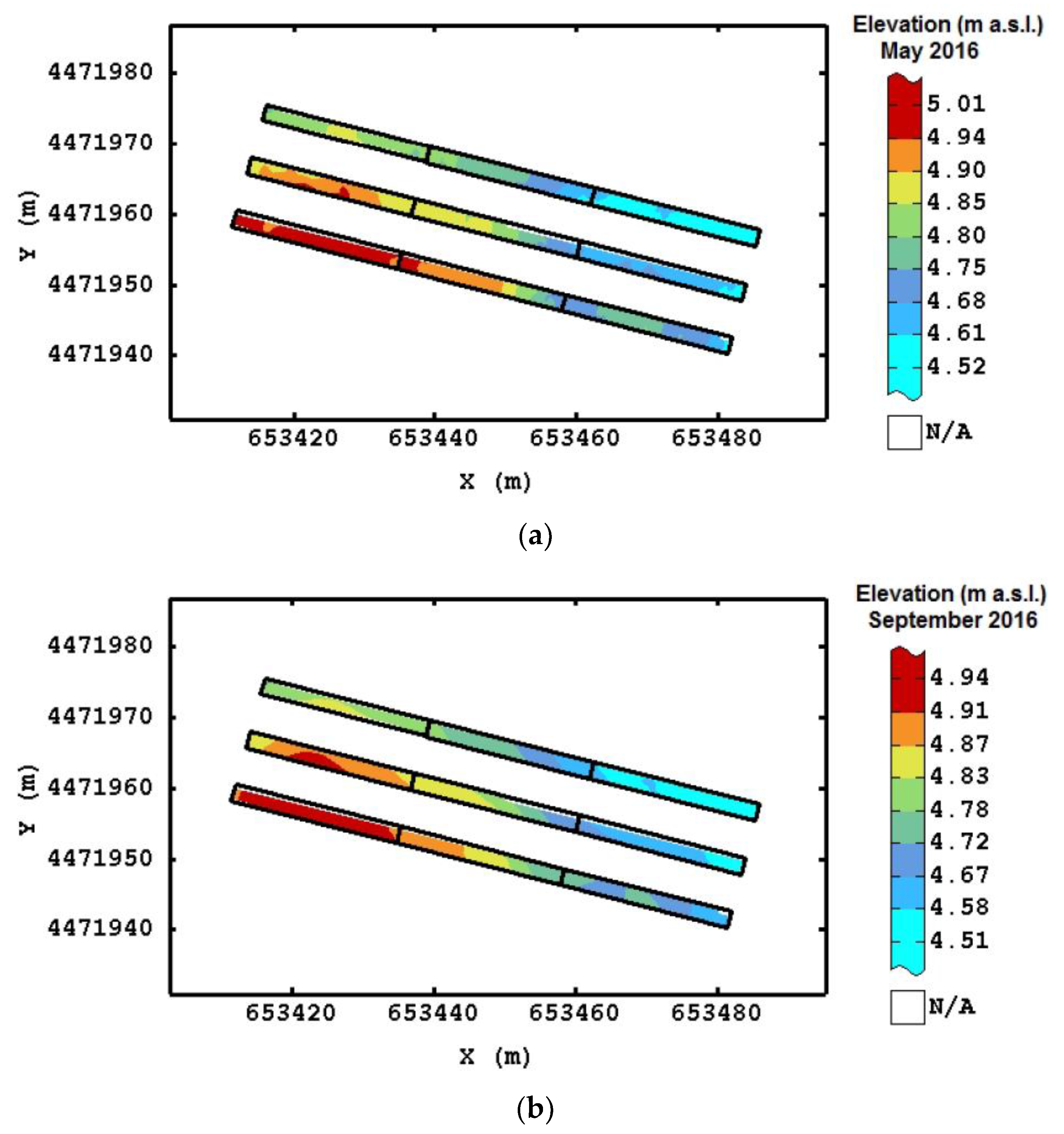
All the obtained maps showed an area with higher values of elevation in the western portion of the field (Figure 5), a central part with intermediate values and the area with lower values located in the eastern side. The map of the estimated elevation for February 2017 (Figure 5c) was more smoothed compared with the ones of the previous surveys because of coarse sampling.
Variation in absolute values was registered and, in particular, a reduction in elevation values was observed. However, spatial structures were not modified following the rainfall event and the depression along the eastern part of the field was maintained, confirming the trend reported in Figure 3.
Combining the statistical and spatial results, a difference in height was observed before the rainfall event, which was also detectable after the event. The lower part of the field (the R3 and in particular the second and third blocks) underwent the major soil loss; therefore, the performed soil hydraulic arrangement did not completely eliminate the risk of water stagnation and did not support the lateral outflow of the excess water [38].
Since the statistical results showed significant difference only for the dates of surveying September 2016 and February 2017, a new grid with the elevation difference (Figure 6) was calculated by subtracting these two DEMs. This map clearly showed that a decrease of elevation (positive difference values) occurred in all ridges. In particular, the eastern part of the field, where a depression was always evident, was subjected to a major decrease, while the R1, characterized by permanent intercropping, showed a more uniform decrease of elevation in comparison with the other soil strips characterized by higher variability. As a consequence, the presence of a permanent cover crop, playing an important role in reducing water and soil losses [39,40], could ensure a greater soil and crop uniformity, which is the base of crop production stability.
3.4. Topographic Data in the Flat Strips
The exploratory analysis of the elevation data in the FS (Table 3), for each survey date, showed an increase of elevation from the first survey in April 2016 to the last one in October 2017. The elevation mean values in the flat strips were lower than those in the raised beds before the artificial event, whereas after it the mean values in the flat strips increased as a result of sediment deposition.
The data distributions were skewed with deviations from the normal distribution, except for the data in the FS1 in October; however, non-parametric tests were applied to assess whether the elevation data for the different survey dates were statistically different.
The differences were not significant in all strips before the extreme rainfall event (between April and October 2016), indicating that there were no changes in elevation in the experimental field and the slight differences may be due both to instrumental errors and/or the normal difference of the field as a results of agronomic practices. Significant differences were found in all FS, after the rainfall event (Table 3e). As a mean value, in March 2017 the FS1 was higher than FS4 by 18.4 cm, suggesting a movement of the deposition towards that part of the field experiment.
As observed in the ridges, the different fertilizer treatments did not affect the elevation in flat strips (data not shown), indicating that also in this case the benefit of organic amendment application did not overcome the limits imposed by the intensity of rainfall [36].
Figure 7 shows that before the event (in October 2016) the elevation values were uniformly distributed within each strip (on almost straight line) and a gradient was present from the first strip to the last one. In March 2017 (after the event), the elevation trend differed from that of October 2016 and it was very similar to the one observed for the ridges (Figure 3), maintaining the differences between the first and the last strip. Considering the absolute values of March 2017, the average height of the FS4, characterized by no-ASC control, underwent an increase of 2.6 cm more than the FS1. From an agronomical point of view, this result suggests that the repeated strong rainfall events could create or increase a soil slope which could influence the level and stability of yield production [17].
3.5. Spatial Variability in the Flat Strips
Also for the FS, the spatial variability within the field was assessed. The data were transformed by Gaussian anamorphosis and the experimental variograms for each date were fit. Finally, the elevation data were interpolated with kriging and thematic maps were produced (Figure 8).
The maps showed a depression along the eastern part of the field and the higher values of elevation in the western corner. Again, the spatial structures were not modified after the rainfall event and significant variation in absolute values was observed in March 2017.
Since the difference was significant only for the surveying dates of October 2016 and March 2017, the elevation changes were calculated from subtraction of these two DEMs (Figure 9). The negative difference values indicated an increase of elevation in all plots; therefore, all FS increased. In particular, the central part of the FS2 and FS3 was characterized by the highest raising (or deposition of sediment), following the outflow line [38]. In the FS4, characterized by no-ASC, there was a more uniform increase of elevation in comparison with the other strips where the variability was higher. These results could also be due to the soil erosion that occurred in the R1 and R2, which were higher than R3; therefore, the rainfall event may be caused a different deposition of sediments. Furthermore, it should be pointed out that the FS4 is close to the R3, which is characterized by the absence of LM that could influence soil water balance and determine loss of sediment [41].
3.6. Soil Losses and Yield
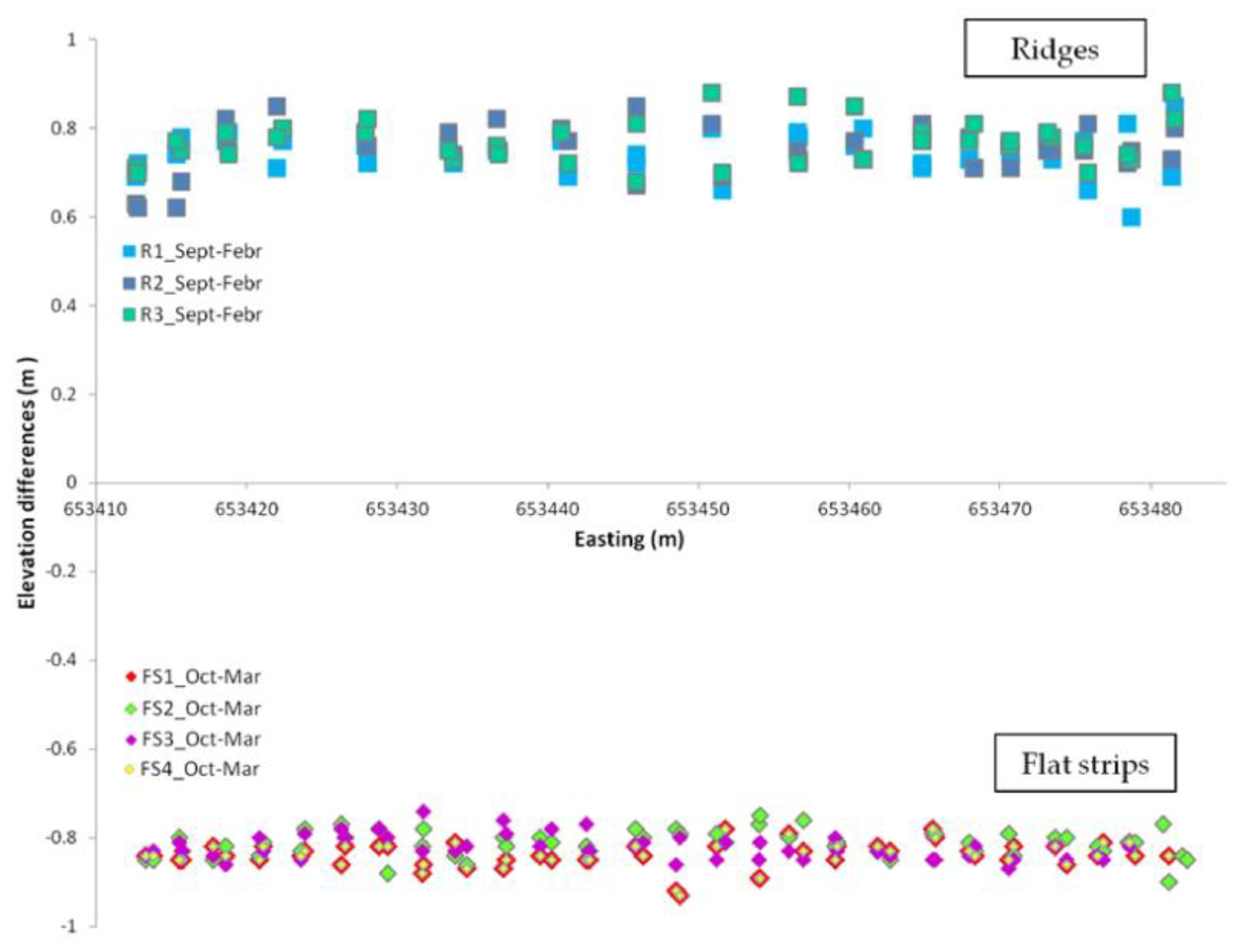
In Figure 10 the elevation difference of each ridge and flat strip is reported, showing that in the R there was higher variability, while in the FS the variation of elevation appeared more uniform. In addition, the figure highlights that the reduction of altitude (or soil loss) in the R was recovered in the FS: all values were allocated in the same range (0.6–0.8 m for the R and from −0.6 to −0.8 m for the FS).
Since the deposition occurred preferentially at the lowest areas of the field experiment (Figure 9), close to the southern border and in the central part of the field following the drainage ways, after the extreme rainfall event, the hydraulic arrangement “ridges-flat strips” was reduced and the ridges were flatten.
The permanent intercropping on the R reduced soil losses compared to the losses that occurred in the R without permanent intercropping. However, the main function of the R was to facilitate the surface runoff after the extreme event, but, in the present case, it did not retain sediments which were transported to the near FS, even if in different ways according with the presence of LM. In any case, under other topographic conditions and without this arrangement, the sediments would have been transported out of the field via drainage and the soil loss would have been increased after an similar extreme event. Although sediment detachment and transport process are different concepts and are controlled by different properties [37], this is an important factor in the future redesign of the hydraulic arrangement in the experimental device.
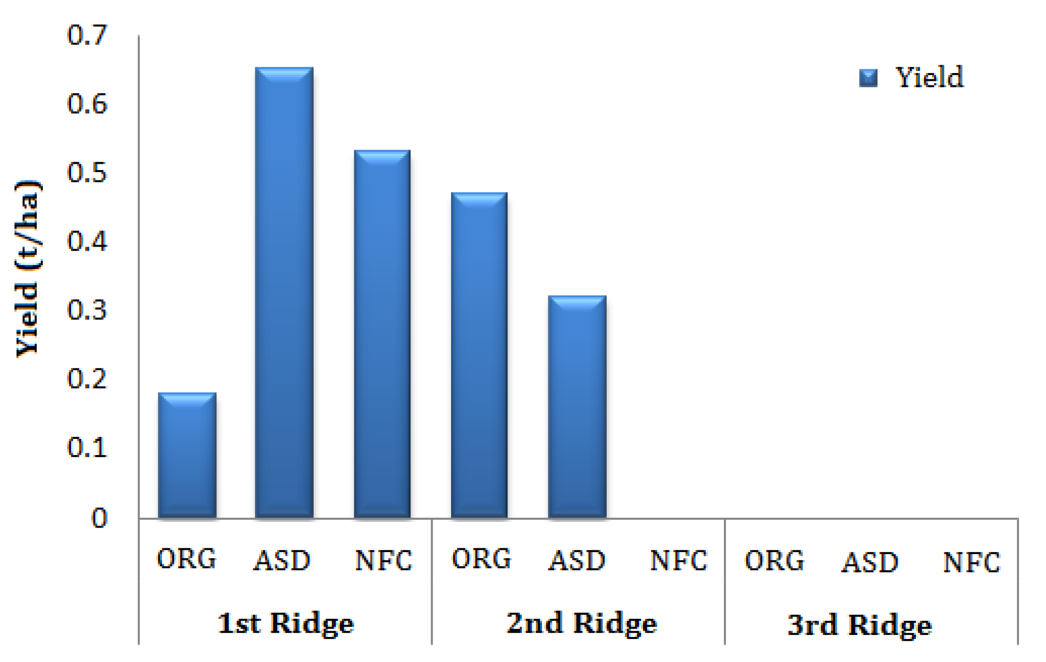
Because crop yields may be sensitive to extreme soil water contents [42], to evaluate the effect of the artificial rainfall event on the yield in the ridges, cash crop yield was determined. Cauliflower marketable yield results showed that crop production was obtained only in the first two ridges (Figure 11). By contrast, in the R3, characterized by absence of mulching and by the highest soil loss, there was no production. In particular, this result could be due to both a higher flooding and a lower soil fertility. This latter aspect could be due to the absence of leguminous cover corps (burr medic and crimson clover) and/or the organic amendments, which generally reduce crop productivity [43]. In particular, after the extreme rainfall event, the R3 remained flooded for a longer time period (about 3–4 days) as compared to the R1 and R2, which were characterized by waterlogging of about 2–3 days. Furthermore, the natural rainfall that occurred in January 2017 (117 mm) induced a further stress in the cauliflower plants, with a higher influence in R3.
The results connected with zero yield in R3 may be due to flow accumulation and water distribution in the field and can also be dependent on topographic conditions (elevation and slope). In fact, in this case, the yield was zero in the depression along the eastern part of the field experiment. Even if it is not possible to attribute the zero yield, as a unique effect, to the soil erosion and flooding, the results of this research pointed out that the R3 showed, as mean value, a lower height than the R1, which means that in this part of field experiment the soil erosion was higher. As a consequence, the higher flooding which occurred in R3 influenced the cauliflower crop response [44]. In particular, the findings of this research indicated that the combination of both water flooding and soil erosion overcomes the potential beneficial effect of the conservation agriculture practices, i.e., the organic matter distribution in R3 and no permanent intercropping in R2. In fact, no cauliflower yield was recorded in all fertilizer treatments in R3, and in NFC in R2. Conversely, the combination of the tested agronomical practices (LM and organic fertilizers distribution) reduced the negative effect of heavy rainfall, since the production was obtained when these techniques were applied.
4. Conclusions
During the first crop growth period, rainfall did not cause significant soil altitude differences (soil losses) because the quantity was not excessive and water infiltrated. Conversely, in the second period, substantial altitude differences were found as a consequence of the extreme artificial rainfall event, which caused soil erosion in the ridges and deposition in the strips.
In particular, the results of this research indicated that the presence of LM in R1 reduces soil losses and consequently maintains the level of crop productivity even if there is a very important rainfall event. In fact, as an absolute value and after a whole cropping system and one artificial heavy rainfall event, the mean value of R1 was 13 cm higher than R3, while the R2 showed an intermediate behavior. These findings indicated that LM on the ridges reduced soil losses compared to the losses that occurred in the ridges without permanent intercropping. From an agronomic point of view, this conservative practice could also reduce soil organic matter loss and ensure crop production, even in the presence of climatic change context which could cause extreme rainfall events and consequently, temporary flooding.
In light of the fact that there is an increase of precipitation extremes separated by long dry periods, the study has proved the high erosive potential of the extreme events and the significant economic losses to farmers. However, future work should focus on the influence of runoff and soil losses on nutrient transport.
Acknowledgments
This paper is a result of the AGROCAMBIO (Sistemi e tecniche AGROnomiche di adattamento ai CAMbiamenti climatici in sistemi agricoli BIOlogici) and RETIBIO (Attività di supporto nel settore dell’agricoltura biologica per il mantenimento dei dispositivi sperimentali di lungo termine e il rafforzamento delle reti di relazioni esistenti a livello nazionale e internazionale) research projects funded by the Organic Farming Office of the Italian Ministry of Agriculture.
Author Contributions
Francesco Montemurro and Mariangela Diacono conceived and designed the Mitiorg experimental device and performed the field experiments; Daniela De Benedetto performed the surveys, statistical and geostatistical analysis. All authors equally contributed to the design and drafting of this paper.
Conflicts of Interest
The authors declare no conflict of interest.
References
- Bellard, C.; Bertelsmeier, C.; Leadley, P.; Thuiller, W.; Courchamp, F. Impacts of climate change on the future of biodiversity. Ecol. Lett. 2012, 15, 365–377. [Google Scholar] [CrossRef] [PubMed]
- García-Ruiz, J.M.; Nadal-Romero, E.; Lana-Renault, N.; Beguería, S. Erosion in Mediterranean landscapes: Changes and future challenges. Geomorphology 2013, 198, 20–36. [Google Scholar] [CrossRef] [Green Version]
- Rodrigo-Comino, J.; Senciales González, J.M.; Ramos, M.C.; Martínez-Casasnovas, J.A.; Lasanta Martínez, T.; Brevik, E.C.; Ries, J.B.; Ruiz-Sinoga, J.D. Understanding soil erosion processes in Mediterranean sloping vineyards (Montes de Málaga, Spain). Geoderma 2017, 296, 47–59. [Google Scholar] [CrossRef]
- Martínez-Casasnovas, J.A.; Ramos, M.C.; Ribes-Dasi, M. Soil erosion caused by extreme rainfall events: Mapping and quantification in agricultural plots from very detailed digital elevation models. Geoderma 2002, 105, 125–140. [Google Scholar] [CrossRef]
- Boardman, J.; Poesen, J.; Evans, R. Socio-economic factors in soil erosion and conservation. Environ. Sci. Policy 2003, 6, 1–6. [Google Scholar] [CrossRef]
- Food and Agriculture Organization of the United Nations (FAO). Agroecology to Reverse Soil Degradation and Achieve Food Security. 2015. Available online: http://www.fao.org/soils-2015/news/news-detail/en/c/317402/ (accessed on 24 July 2017).
- Tilman, D.; Cassman, K.G.; Matson, P.A.; Naylor, R.; Polasky, S. Agricultural sustainability and intensive production practices. Nature 2002, 418, 671–677. [Google Scholar] [CrossRef] [PubMed]
- Ismail, I.; Blevins, R.L.; Frye, W.W. Long-term no-tillage effects on soil properties and continuous corn yields. Soil Sci. Soc. Am. J. 1994, 58, 193–198. [Google Scholar] [CrossRef]
- Montemurro, F.; Ciaccia, C.; Leogrande, R.; Ceglie, F.; Diacono, M. Suitability of different organic amendments from agro-industrial wastes in organic lettuce crops. Nutr. Cycl. Agroecosyst. 2015, 102, 243–252. [Google Scholar] [CrossRef]
- Diacono, M.; Montemurro, F. Long-term effects of organic amendments on soil fertility. A review. Agron. Sustain. Dev. 2010, 30, 401–422. [Google Scholar] [CrossRef]
- Mijatović, D.; Van Oudenhoven, F.; Eyzaguirre, P.; Hodgkin, T. The role of agricultural biodiversity in strengthening resilience to climate change: Towards an analytical framework. Int. J. Agric. Sustain. 2013, 11, 95–107. [Google Scholar] [CrossRef]
- Cerdà, A.; Rodrigo-Comino, J.; Giménez Morera, A.; Keesstra, S.D. An economic, perception and biophysical approach to the use of oat straw as mulch in Mediterranean rainfed agriculture land. Ecol. Eng. 2017, 108, 162–171. [Google Scholar] [CrossRef]
- Meynard, J.M.; Messéan, A.; Charlier, A.; Charrier, F.; Fares, M.; Le Bail, M.; Magrini, M.B.; Savini, I. Brakes and levers to diversification of cultures in France: Study of agricultural farms and chains. OCL Oilseeds Fats Crop. Lipids 2013, 20, D403. [Google Scholar] [CrossRef]
- Montemurro, F.; Diacono, M.; Ciaccia, C.; Campanelli, G.; Tittarelli, F.; Leteo, F.; Canali, F. Effectiveness of living mulch strategies for winter organic cauliflower (Brassica oleracea L. var. botrytis) production in Central and Southern Italy. Renew. Agric. Food Syst. 2017, 32, 263–272. [Google Scholar] [CrossRef]
- Canali, S.; Campanelli, G.; Ciaccia, C.; Leteo, F.; Testani, E.; Montemurro, F. Conservation tillage strategy based on the roller crimper technology for weed control in Mediterranean vegetable organic cropping systems. Eur. J. Agron. 2013, 50, 11–18. [Google Scholar] [CrossRef]
- Yang, C.; Peterson, C.L.; Shropshire, G.J.; Otawa, T. Spatial variability of field topography and wheat yield in the Palouse Region of the Pacific Northwest. Trans. Am. Soc. Agric. Eng. 1998, 41, 17–27. [Google Scholar] [CrossRef]
- Marques da Silva, J.R.; Alexandre, C. Spatial variability of irrigated corn yield in relation to field topography and soil chemical characteristics. Precis. Agric. 2005, 6, 453–466. [Google Scholar] [CrossRef]
- Rodrigo-Comino, J.; Cerdà, A. Improving stock unearthing method to measure soil erosion rates in vineyards. Ecol. Indic. 2018, 85, 509–517. [Google Scholar] [CrossRef]
- Dosskey, M.G.; Eisenhauer, D.E.; Helmers, M.J. Establishing conservation buffers using precision information. J. Soil Water Conserv. 2005, 60, 349–354. [Google Scholar]
- Renschler, C.S.; Flanagan, D.C. Site-specific decision-making based on RTK GPS survey and six alternative elevation data sources: Soil erosion predictions. Trans. Am. Soc. Agric. Biol. Eng. 2008, 51, 413–424. [Google Scholar] [CrossRef]
- Westphalen, M.L.; Steward, B.S.; Han, S. Topographic mapping through measurement of vehicle attitude and elevation. Trans. Am. Soc. Agric. Eng. 2004, 47, 1841–1849. [Google Scholar] [CrossRef]
- Diacono, M.; Persiani, A.; Fiore, A.; Montemurro, F.; Canali, S. Agro-ecology for potential adaptation of horticultural systems to climate change: Agronomic and energetic performance evaluation. Agronomy 2017, 7, 35. [Google Scholar] [CrossRef]
- Soil Survey Staff. Soil taxonomy. In Agriculture Handbook 436; USDA-NRCS: Washington, DC, USA, 1999. [Google Scholar]
- Unesco-FAO. Etude Écologique de la Zone Méditerranéenne. Carte Bioclimatique de la Zone Méditerranéenne (Ecological Study of the Mediterranean Area: Bioclimatic Map of the Mediterranean Sea). Paris-Rome. 1963. Available online: http://unesdoc.unesco.org/images/0013/001372/137255fo.pdf (accessed on 19 October 2017).
- Diacono, M.; Fiore, A.; Farina, R.; Canali, S.; Di Bene, C.; Testani, E.; Montemurro, F. Combined agro-ecological strategies for adaptation of organic horticultural systems to climate change in Mediterranean environment. Ital. J. Agron. 2016, 11, 85–91. [Google Scholar] [CrossRef]
- Decree, L. Riordino e Revisione della Disciplina in Materia di Fertilizzanti, a Norma Dell’articolo 13 della Legge 7 Luglio 2009, n. 88; Gazzetta Ufficiale n. 121 26/05/2010, 26 May 2010; Istituto Poligrafico e Zecca dello Stato: Rome, Italia, 2010. (In Italian) [Google Scholar]
- Chiles, J.P.; Delfiner, P. Geostatistics: Modeling Spatial Uncertainty; Wiley & Sons: New York, NY, USA, 1999; 695p, ISBN 978-0470183151. [Google Scholar]
- Wackernagel, H. Multivariate Geostatistics: An Introduction with Applications, 3rd ed.; Springer: Berlin, Germany, 2003; 388p, ISBN 3540441425. [Google Scholar]
- Goovaerts, P. Geostatistics for Natural Resources Evaluation; Oxford University Press: New York, NY, USA, 1997; ISBN 0-19-511538-4. [Google Scholar]
- Geovariances. Isatis Technical Ref. Ver. 2013.1; Geovariances & Ecole Des Mines De Paris: Avon Cedex, France, 2015. [Google Scholar]
- Wechsler, S.P. Uncertainties associated with digital elevation models for hydrologic applications: A review. Hydrol. Earth Syst. Sci. 2007, 11, 1481–1500. [Google Scholar] [CrossRef]
- Sojika, R.E.; Langdale, G.W.; Karlen, D.L. Vegetative techniques for reducing water erosion of cropland in the southeastern United States. Adv. Agron. 1984, 37, 155–181. [Google Scholar] [CrossRef]
- Dabney, S.M.; Delgado, J.A.; Reeves, D.W. Using winter cover crops to improve soil and water quality. Commun. Soil Sci. Plant Anal. 2001, 32, 1221–1250. [Google Scholar] [CrossRef]
- Leary, J.; DeFrank, J. Living mulches for organic farming systems. HortTechnology 2000, 10, 692–698. [Google Scholar]
- Kaspar, T.C.; Radke, J.K.; Laflen, J.M. Small grain cover crops and wheel traffic effects on infiltration, runoff, and erosion. J. Soil Water Conserv. 2001, 56, 160–164. [Google Scholar]
- Ramos, M.C.; Martínez-Casasnovas, J.A. Erosion rates and nutrient losses affected by composted cattle manure application in vineyard soils of NE Spain. CATENA 2006, 68, 177–185. [Google Scholar] [CrossRef]
- Jacinthe, P.A.; Lal, R.; Kimble, J.M. Carbon dioxide evolution in runoff from simulated rainfall on long-term no-till and plowed soils in southwestern Ohio. Soil Tillage Res. 2001, 66, 23–33. [Google Scholar] [CrossRef]
- De Benedetto, D.; Montemurro, F.; Diacono, M. Geophysical Sensors to Characterise an Agricultural Experimental Device and to Improve Soil Water Content Estimation. NJAS Wagening. J. Life Sci. 2017. under review. [Google Scholar]
- Tropeano, D. Rate of soil erosion processes on vineyards in central Piedmont (NW Italy). Earth Surf. Process. Landf. 1984, 9, 253–266. [Google Scholar] [CrossRef]
- Corti, G.; Cavallo, E.; Cocco, S.; Biddoccu, M.; Brecciaroli, G.; Agnelli, A. Evaluation of Erosion Intensity and Some of Its Consequences in Vineyards from Two Hilly Environments under a Mediterranean Type of Climate, Italy. In Soil Erosion Issues in Agriculture; Godone, D., Stanchi, S., Eds.; InTech: London, UK, 2011; 346p, ISBN 978-953-307-435-1. [Google Scholar]
- Vahabi, J.; Nikkami, D. Assessing dominant factors affecting soil erosion using a portable rainfall simulator. Int. J. Sediment Res. 2008, 23, 376–386. [Google Scholar] [CrossRef]
- Bakker, M.M.; Govers, G.; Jones, R.A.; Rounsevell, M.D. The Effect of Soil Erosion on Europe’s Crop Yields. Ecosystems 2007, 10, 1209–1219. [Google Scholar] [CrossRef]
- Montemurro, F.; Fiore, A.; Campanelli, G.; Tittarelli, F.; Ledda, L.; Canali, S. Organic fertilization, green manure, and vetch mulch to improve organic zucchini yield and quality. HortScience 2013, 48, 1027–1033. [Google Scholar]
- Rao, R.; Li, Y. Management of flooding effects on growth of vegetable and selected field crops. HortTechnology 2003, 13, 610–616. [Google Scholar]
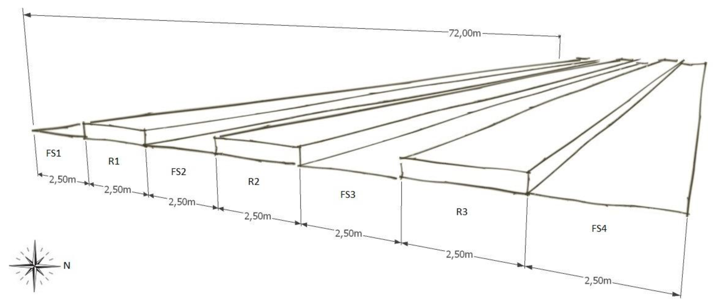
Figure 1.
General layout of the experimental field indicating the soil surface shaping, with four flat areas (FS1–4) and three raised beds (R1–3). This is the innovative MITIORG organic long-term field experiment (Long-term climatic change adaptation in organic farming: synergistic combination of hydraulic arrangement, crop rotations, agro-ecological service crops and agronomic techniques), located on the research farm ‘Azienda Sperimentale Metaponto’ of the Council for Agricultural Research and Economics, Research Centre for Agriculture and Environment (CREA-AA) (Metaponto—MT, Italy; lat. 40°24′ N; long. 16°48′ E). 2,50 m = 2.50 m; 72,00 m = 72.00 m.

Figure 2.
The experimental device with the sampling location based on a kinematic (black points) and punctual (red triangles) approach, along the four flat strips (FS) and the three ridges (R) split in the three different fertilizations. For each ridge, the cash crop (CC) was cultivated with different types of legume LM (LM1 and LM2) and with no living mulch control (NMC). For each FS, the ASC mixtures were cultivated (MIX1, MIX2) and a no ASC control (NAC) was also included.
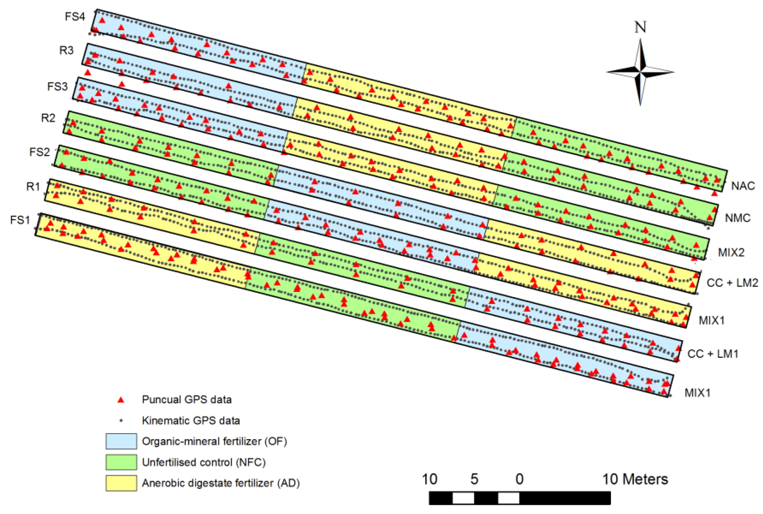
Figure 3.
Mean monthly temperature and cumulative rainfall at the study site in the trial period (January 2016 and March 2017). The arrows indicate the date of the survey carried out in the FS (green arrows) and in the R (black arrows). The red arrow indicates the month of the extreme rainfall event.
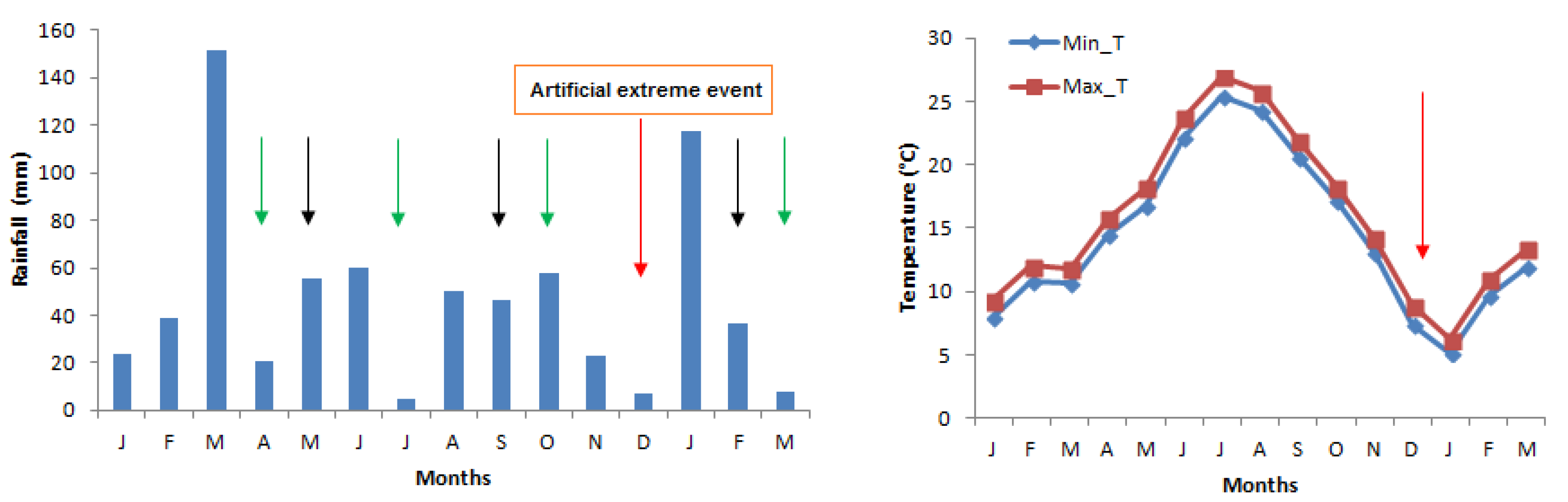
Figure 4.
Trend of the three ridges for September 2016 and February 2017, before and after the extreme event, respectively.
Figure 4.
Trend of the three ridges for September 2016 and February 2017, before and after the extreme event, respectively.
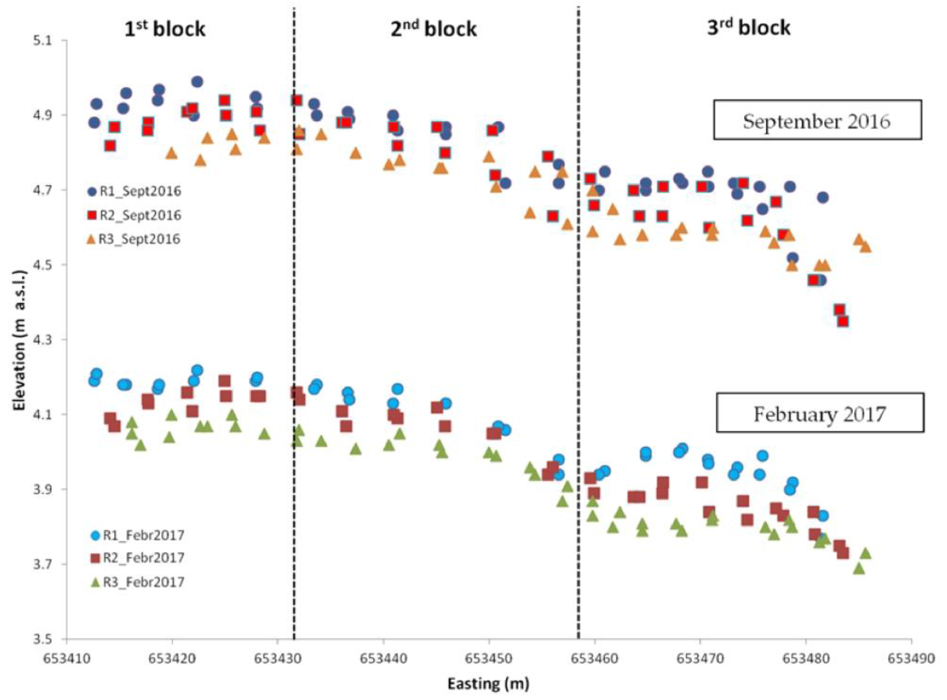
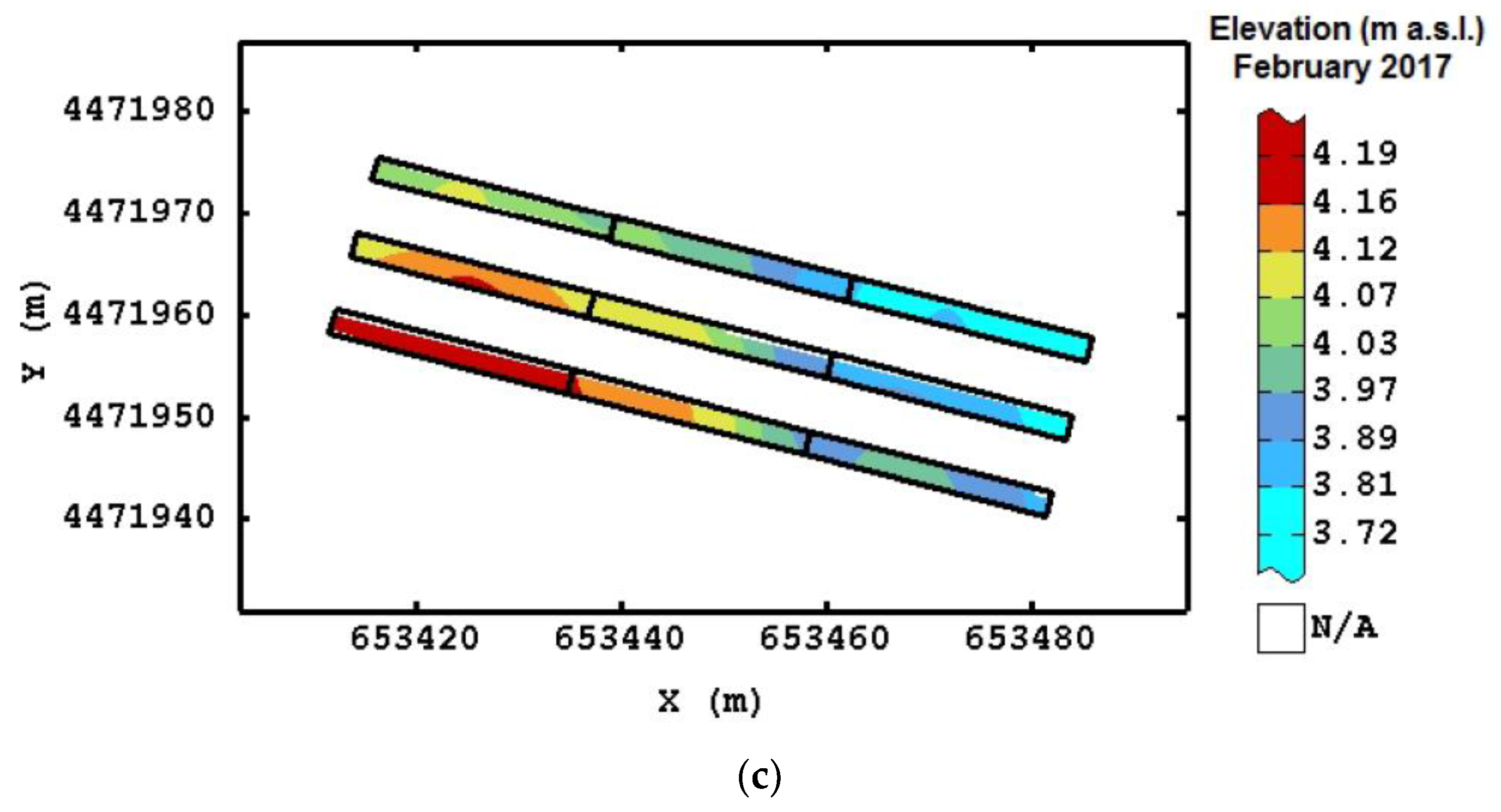
Figure 5.
Spatial estimate of elevation in May 2016 (a); September 2016 (b) and February 2017 (c). Color scale uses iso-frequency classes.
Figure 5.
Spatial estimate of elevation in May 2016 (a); September 2016 (b) and February 2017 (c). Color scale uses iso-frequency classes.


Figure 6.
Map of the elevation differences between the estimated elevation in September 2016 and in February 2017.
Figure 6.
Map of the elevation differences between the estimated elevation in September 2016 and in February 2017.
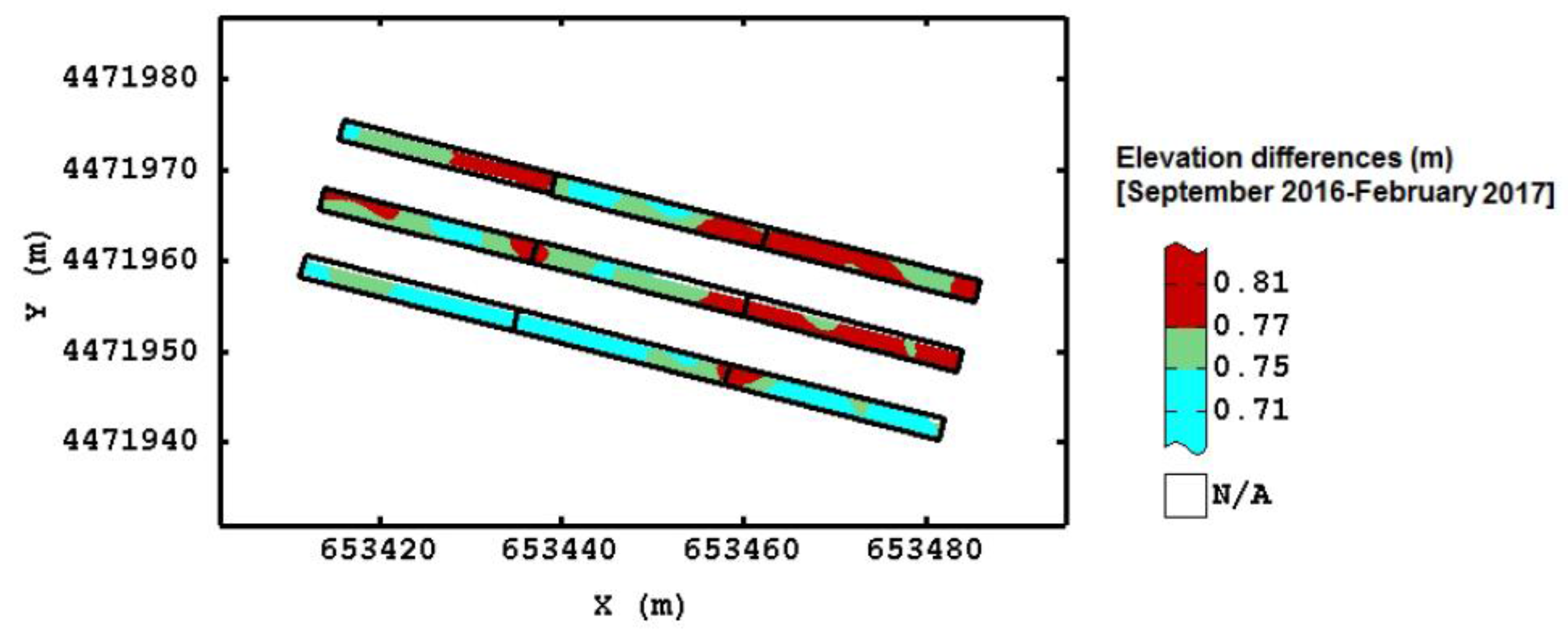
Figure 7.
Trend of the four flat strips for October 2016 and March 2017, before and after the extreme events, respectively.
Figure 7.
Trend of the four flat strips for October 2016 and March 2017, before and after the extreme events, respectively.
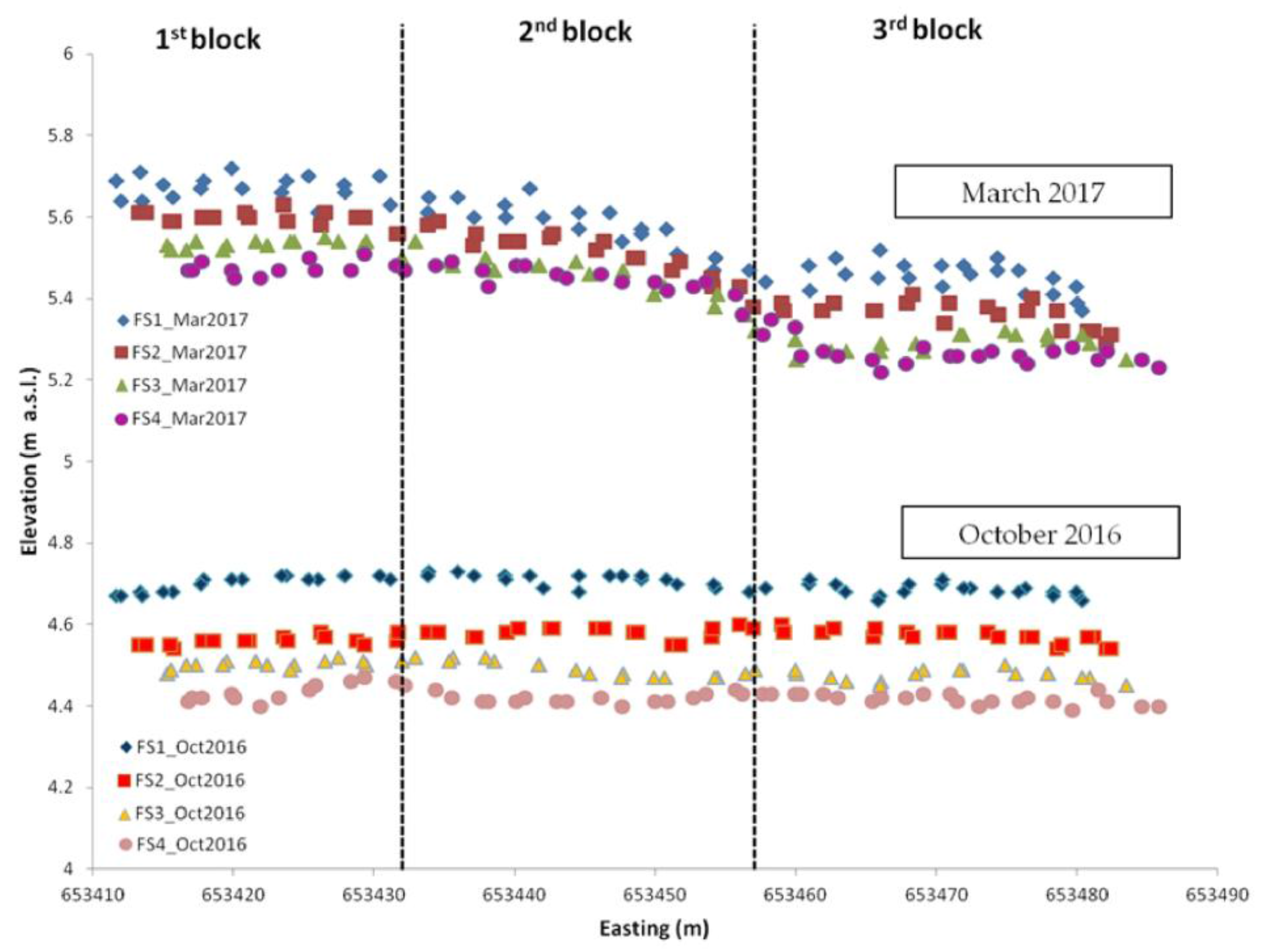
Figure 8.
Spatial estimate of elevation in April 2016 (a); July 2016 (b); October 2016 (c) and March 2017 (d). Color scale uses iso-frequency classes.
Figure 8.
Spatial estimate of elevation in April 2016 (a); July 2016 (b); October 2016 (c) and March 2017 (d). Color scale uses iso-frequency classes.
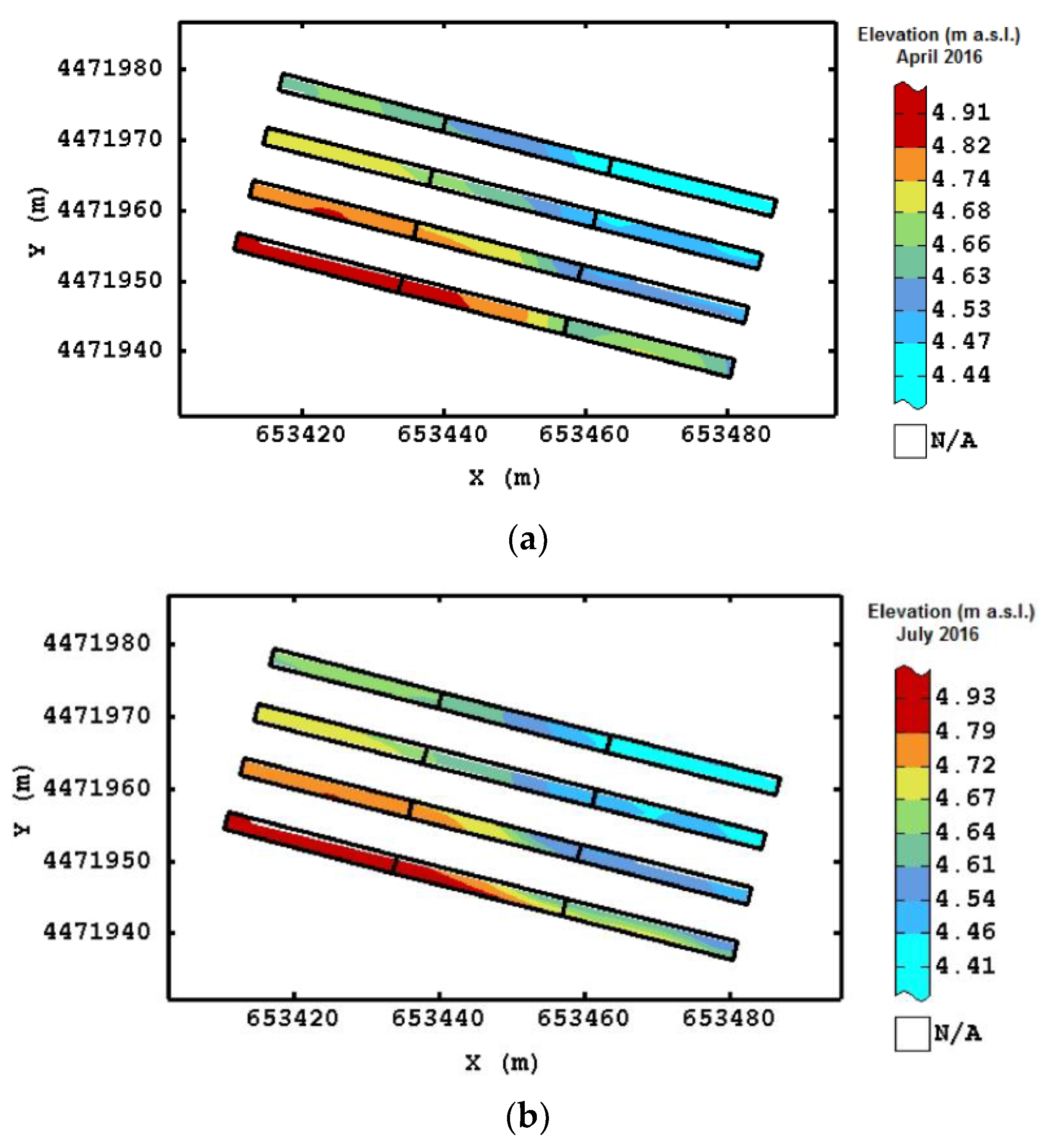
Figure 9.
Map of the elevation differences (in meters) between the estimated elevation in October 2016 and in March 2017.
Figure 9.
Map of the elevation differences (in meters) between the estimated elevation in October 2016 and in March 2017.
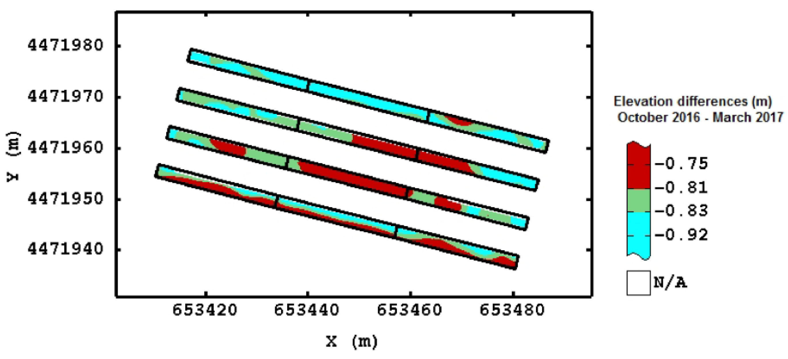
Figure 10.
Elevation differences for each ridge (R) before and after the extreme rainfall event (September and February, respectively) and the elevation difference for each flat strip (FS) before and after the extreme rainfall event (October and March, respectively).
Figure 10.
Elevation differences for each ridge (R) before and after the extreme rainfall event (September and February, respectively) and the elevation difference for each flat strip (FS) before and after the extreme rainfall event (October and March, respectively).

Figure 11.
Mean values of marketable yield (t ha−1) for each treatment with three different fertilizations (ORG = organic fertilizer, NFC = unfertilized control, ASD = anaerobic digestate fertilizer).
Figure 11.
Mean values of marketable yield (t ha−1) for each treatment with three different fertilizations (ORG = organic fertilizer, NFC = unfertilized control, ASD = anaerobic digestate fertilizer).

Table 1.
Descriptive statistics of elevation (m a.s.l.) for (a) the first ridge (intercropping cauliflower crop and burr medic living mulch—LM), (b) the second ridge (intercropping cauliflower crop and crimson clover LM) and (c) the third ridge (no LM control) in May 2016, September 2016 and February 2017. Results of the Mann-Whitney test (d).
| (a) | |||||||
| Date of Survey | Observation | Ridge 1 | |||||
| Min | Max | Mean | Skewness | Kurtosis | Pr < W † | ||
| May 2016 | 38 | 4.570 | 4.990 | 4.846 | −0.469 | 2.159 | 0.001 |
| September 2016 | 38 | 4.462 | 4.987 | 4.802 | −0.569 | 2.818 | 0.006 |
| February 2017 | 38 | 3.774 | 4.225 | 4.059 | −0.357 | 2.012 | 0.003 |
| (b) | |||||||
| Date of Survey | Observation | Ridge 2 | |||||
| Min | Max | Mean | Skewness | Kurtosis | Pr < W † | ||
| May 2016 | 38 | 4.600 | 4.950 | 4.786 | −0.184 | 1.402 | <0.0001 |
| September 2016 | 38 | 4.349 | 4.942 | 4.746 | −0.868 | 2.951 | 0.003 |
| February 2017 | 38 | 3.726 | 4.189 | 3.994 | −0.285 | 1.652 | 0.004 |
| (c) | |||||||
| Date of Survey | Observation | Ridge 3 | |||||
| Min | Max | Mean | Skewness | Kurtosis | Pr < W † | ||
| May 2016 | 42 | 4.520 | 4.860 | 4.711 | −0.159 | 1.406 | <0.0001 |
| September 2016 | 42 | 4.497 | 4.856 | 4.690 | −0.120 | 1.558 | 0.002 |
| February 2017 | 42 | 3.693 | 4.097 | 3.925 | −0.144 | 1.478 | 0.001 |
| (d) | |||||||
| Date of Survey | Average Differences (m) | ||||||
| Ridge 1 | Ridge 2 | Ridge 3 | |||||
| May 2016–September 2016 | 0.044 * | 0.040 ns | 0.021 ns | ||||
| September 2016–February 2017 | 0.743 ** | 0.753 * | 0.765 * | ||||
† Shapiro–Wilk test (W) significant at the p ≤ 0.05 level shown in bold; *, ** Significant at the p ≤ 0.05, 0.01 levels respectively, ns = not significant.
Table 2.
Average differences between the mean elevation values for each ridge considering the different treatments (OF, organic fertilizer; AD, anaerobic digestate fertilizer; NFC, unfertilized control) and the results of the Mann-Whitney test.
Table 2.
Average differences between the mean elevation values for each ridge considering the different treatments (OF, organic fertilizer; AD, anaerobic digestate fertilizer; NFC, unfertilized control) and the results of the Mann-Whitney test.
| Ridge | Treatments | Average Differences (m) | |
|---|---|---|---|
| May 2016–September 2016 | September 2016–February 2017 | ||
| Ridge 1 | NFC | 0.049 ns | 0.745 * |
| AD | 0.038 * | 0.744 * | |
| OF | 0.044 * | 0.739 * | |
| Ridge 2 | NFC | 0.022 ns | 0.757 * |
| AD | 0.065 ns | 0.744 * | |
| OF | 0.026 ns | 0.757 * | |
| Ridge 3 | NFC | 0.018 ns | 0.776 * |
| AD | 0.020 ns | 0.766 * | |
| OF | 0.021 ns | 0.751* | |
* Significant at the p ≤ 0.05 level, ns = not significant.
Table 3.
Descriptive statistics of elevation (m a.s.l.) for (a) the first; (b) second; (c) third and (d) fourth (no LM control) strip in April 2016, July 2016, October 2016 and February 2017. Results of the Mann-Whitney test (e).
Table 3.
Descriptive statistics of elevation (m a.s.l.) for (a) the first; (b) second; (c) third and (d) fourth (no LM control) strip in April 2016, July 2016, October 2016 and February 2017. Results of the Mann-Whitney test (e).
| (a) | |||||||
| Date of Survey | Observation | Flat Strip 1 | |||||
| Min | Max | Mean | Skewness | Kurtosis | Pr < W † | ||
| April 2016 | 59 | 4.550 | 4.920 | 4.768 | −0.175 | 1.634 | 0.0002 |
| July 2016 | 59 | 4.489 | 4.938 | 4.758 | −0.668 | 3.193 | 0.022 |
| October 2016 | 59 | 4.537 | 4.913 | 4.746 | −0.222 | 2.354 | 0.229 |
| March 2017 | 59 | 5.368 | 5.721 | 5.559 | −0.091 | 1.60 | 0.002 |
| (b) | |||||||
| Date of Survey | Observation | Flat Strip 2 | |||||
| Min | Max | Mean | Skewness | Kurtosis | Pr < W † | ||
| April 2016 | 54 | 4.520 | 4.820 | 4.681 | −0.103 | 1.388 | <0.0001 |
| July 2016 | 54 | 4.387 | 4.811 | 4.660 | 2.031 | 4.659 | 0.0002 |
| October 2016 | 54 | 4.422 | 4.815 | 4.667 | 2.004 | 4.666 | 0.001 |
| March 2017 | 54 | 5.292 | 5.629 | 5.479 | 1.475 | 5.478 | 0.0001 |
| (c) | |||||||
| Date of Survey | Observation | Flat Strip 3 | |||||
| Min | Max | Mean | Skewness | Kurtosis | Pr < W † | ||
| April 2016 | 49 | 4.440 | 4.740 | 4.611 | −0.394 | 1.459 | <0.0001 |
| July 2016 | 49 | 4.382 | 4.714 | 4.586 | −0.310 | 1.614 | 0.0002 |
| October 2016 | 49 | 4.405 | 4.714 | 4.596 | −0.411 | 1.524 | <0.0001 |
| March 2017 | 49 | 5.252 | 5.546 | 5.417 | −0.241 | 1.377 | <0.0001 |
| (d) | |||||||
| Date of Survey | Observation | Flat Strip 4 | |||||
| Min | Max | Mean | Skewness | Kurtosis | Pr < W † | ||
| April 2016 | 51 | 4.410 | 4.690 | 4.557 | −0.095 | 1.354 | <0.0001 |
| July 2016 | 51 | 4.400 | 4.676 | 4.546 | −0.189 | 1.384 | <0.0001 |
| October 2016 | 51 | 4.392 | 4.663 | 4.536 | −0.178 | 1.323 | <0.0001 |
| March 2017 | 51 | 5.220 | 5.506 | 5.375 | −0.249 | 1.287 | <0.0001 |
| (e) | |||||||
| Date of Survey | Average Differences (m) | ||||||
| 1st Flat Strip | 2nd Flat Strip | 3rd Flat Strip | 4th Flat Strip | ||||
| April 2016–July 2016 | 0.0086 ns | 0.020 ns | 0.025 ns | 0.009 ns | |||
| July 2016–October 2016 | 0.020 ns | −0.061 ns | −0.011 ns | 0.010 ns | |||
| October 2016–March 2017 | −0.813 * | −0.812 * | −0.821 * | −0.839 * | |||
† Shapiro–Wilk test (W) significant at the p ≤ 0.05 level in bold; * Significant at the p ≤ 0.05 level, ns = not significant.
© 2017 by the authors. Licensee MDPI, Basel, Switzerland. This article is an open access article distributed under the terms and conditions of the Creative Commons Attribution (CC BY) license (http://creativecommons.org/licenses/by/4.0/).
Share and Cite
MDPI and ACS Style
De Benedetto, D.; Montemurro, F.; Diacono, M. Impacts of Agro-Ecological Practices on Soil Losses and Cash Crop Yield. Agriculture 2017, 7, 103. https://doi.org/10.3390/agriculture7120103
AMA Style
De Benedetto D, Montemurro F, Diacono M. Impacts of Agro-Ecological Practices on Soil Losses and Cash Crop Yield. Agriculture. 2017; 7(12):103. https://doi.org/10.3390/agriculture7120103
Chicago/Turabian StyleDe Benedetto, Daniela, Francesco Montemurro, and Mariangela Diacono. 2017. "Impacts of Agro-Ecological Practices on Soil Losses and Cash Crop Yield" Agriculture 7, no. 12: 103. https://doi.org/10.3390/agriculture7120103
Note that from the first issue of 2016, this journal uses article numbers instead of page numbers. See further details here.