Copy Number Studies in Noisy Samples

Abstract
:1. Introduction
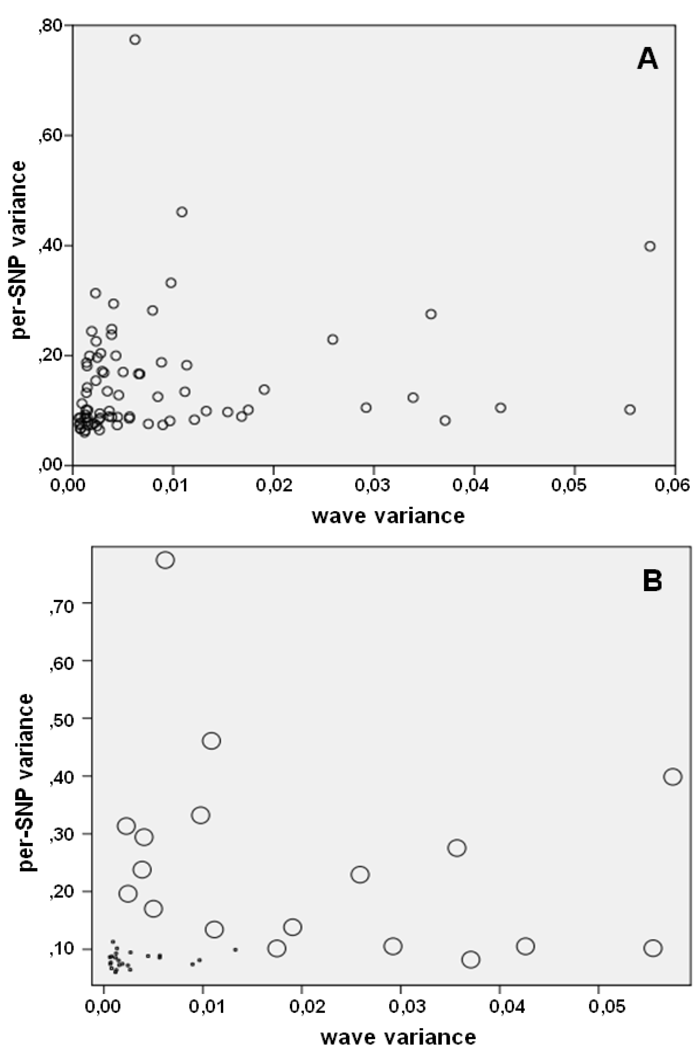
2. Noise Components

3. Factors Associated with Quality of Copy Number Data

| Ineligible | Intermediate | Eligible | Chi-2/ kruskal-wallis | |
|---|---|---|---|---|
| (n = 29) | (n = 25) | (n = 23) | p | |
| Fresh DNA preparation | 0 (0.0 %) | 6 (20.7 %) | 14 (60.9 %) | <0.001 |
| Genotyping call rate | 94.7 [80.9–97.3] | 96.6 [94.8–98.3] | 97.7 [96.6–98.5] | <0.001 |
| Autosomal variance | 0.2291 [0.115–0.706] | 0.1343 [0.068–0.208] | 0.0870 [0.062–0.114] | <0.001 |
| wave noise | 0.0109 [0.002–0.058] | 0.0034 [0.001–0.017] | 0.0015 [0.001–0.013] | <0.001 |
| per–SNP noise | 0.2259 [0.082–0.696] | 0.1281 [0.067–0.204] | 0.0811 [0.060–0.164] | <0.001 |
| PennCNV, No. of calls | 238 [14–1821) | 103 [34–1024] | 98 [63–165] | 0.053 |
| PennCNV, % of deletions | 18.6 [1.3–81.3] | 27.4 [0.7–65.9] | 40.0 [10.3–54.8] | 0.164 |
| Birdview No. of calls | 527 [163–8,203] | 225 [154–1,339] | 208 [163–348] | <0.001 |
| Birdview (cf > 10) | 15 [2–717] | 12 [5–33] | 14 [4–20] | 0.048 |
| Birdview (cf = 10) | 89 [76–145] | 92 [74–105] | 94 [77–102] | 0.209 |
| Birdview (cf 2.5–10) | 93 [14–3344] | 19 [10–361] | 21 [11–45] | <0.001 |
| Birdview (cf < 2.5) | 370 [52–5665] | 106 [35–857] | 85 [42–194] | <0.001 |
4. Noise Reduction in Copy Number Samples
5. Conclusions—Proposal of a Two-Step Procedure for the Validation of CNV Findings
Acknowledgments
Conflicts of Interest
References
- Girirajan, S.; Campbell, C.D.; Eichler, E.E. Human copy number variation and complex genetic disease. Annu. Rev. Genet. 2011, 45, 203–226. [Google Scholar] [CrossRef]
- Zhang, F.; Gu, W.; Hurles, M.E.; Lupski, J.R. Copy number variation in human health, disease, and evolution. Annu. Rev. Genomics Hum. Genet. 2009, 10, 451–481. [Google Scholar] [CrossRef]
- Fakhro, K.A.; Choi, M.; Ware, S.M.; Belmont, J.W.; Towbin, J.A.; Lifton, R.P.; Khokha, M.K.; Brueckner, M. Rare copy number variations in congenital heart disease patients identify unique genes in left-right patterning. Proc. Natl. Acad. Sci. USA 2011, 108, 2915–2920. [Google Scholar] [CrossRef]
- Priebe, L.; Degenhardt, F.; Strohmaier, J.; Breuer, R.; Herms, S.; Witt, S.H.; Hoffmann, P.; Kulbida, R.; Mattheisen, M.; Moebus, S.; et al. Copy number variants in german patients with schizophrenia. PLoS One 2013, 8, e64035. [Google Scholar] [CrossRef]
- Vandeweyer, G.; Kooy, R.F. Detection and interpretation of genomic structural variation in health and disease. Expert. Rev. Mol. Diagn. 2013, 13, 61–82. [Google Scholar] [CrossRef]
- Southard, A.E.; Edelmann, L.J.; Gelb, B.D. Role of copynumber variants in structural birth defects. Pediatrics 2012, 129, 755–763. [Google Scholar] [CrossRef]
- Zhang, D.; Qian, Y.; Akula, N.; Alliey-Rodriguez, N.; Tang, J.; The Bipolar Genome Study; Gershon, E.S.; Liu, C. Accuracy of CNV detection from GWAS data. PLoS One 2011, 6, e14511. [Google Scholar] [CrossRef]
- Dellinger, A.E.; Saw, S.M.; Goh, L.K.; Seielstad, M.; Young, T.L.; Li, Y.J. Comparative analyses of seven algorithms for copy number variant identification from single nucleotide polymorphism arrays. Nucleic Acids Res. 2010, 38, e105. [Google Scholar] [CrossRef]
- Zheng, X.; Shaffer, J.R.; McHugh, C.P.; Laurie, C.C.; Feenstra, B.; Melbye, M.; Murray, J.C.; Marazita, M.L.; Feingold, E. Using family data as a verification standard to evaluate copy number variation calling strategies for genetic association studies. Genet. Epidemiol. 2012, 36, 253–262. [Google Scholar] [CrossRef]
- Marioni, J.C.; Thorne, N.P.; Valsesia, A.; Fitzgerald, T.; Redon, R.; Fiegler, H.; Andrews, T.D.; Stranger, B.E.; Lynch, A.G.; Dermitzakis, E.T.; et al. Breaking the waves: Improved detection of copy number variation from microarray-based comparative genomic hybridization. Genome Biol. 2007, 8, R228. [Google Scholar] [CrossRef]
- Diskin, S.J.; Li, M.; Hou, C.; Yang, S.; Glessner, J.; Hakonarson, H.; Bucan, M.; Maris, J.M.; Wang, K. Adjustment of genomic waves in signal intensities from whole-genome SNP genotyping platforms. Nucleic Acids Res. 2008, 36, e126. [Google Scholar] [CrossRef]
- Van de Wiel, M.A.; Brosens, R.; Eilers, P.H.; Kumps, C.; Meijer, G.A.; Menten, B.; Sistermans, E.; Speleman, F.; Timmerman, M.E.; Ylstra, B. Smoothing waves in array CGH tumor profiles. Bioinformatics 2009, 25, 1099–1104. [Google Scholar] [CrossRef]
- Lee, Y.H.; Ronemus, M.; Kendall, J.; Lakshmi, B.; Leotta, A.; Levy, D.; Esposito, D.; Grubor, V.; Ye, K.; Wigler, M.; et al. Reducing system noise in copynumber data using principal components of self-self hybridizations. Proc. Natl. Acad. Sci. USA 2012, 109, E103–E110. [Google Scholar] [CrossRef]
- Wang, K.; Li, M.; Hadley, D.; Liu, R.; Glessner, J.; Grant, S.F.; Hakonarson, H.; Bucan, M. PennCNV: An integrated hidden Markov model designed for high-resolution copy number variation detection in whole-genome SNP genotyping data. Genome Res. 2007, 17, 1665–1674. [Google Scholar] [CrossRef]
- Korn, J.M.; Kuruvilla, F.G.; McCarroll, S.A.; Wysoker, A.; Nemesh, J.; Cawley, S.; Hubbell, E.; Veitch, J.; Collins, P.J.; Darvishi, K.; et al. Integrated genotype calling and association analysis of SNPs, common copy number polymorphisms and rare CNVs. Nat. Genet. 2008, 40, 1253–1260. [Google Scholar] [CrossRef]
- McCarroll, S.A.; Kuruvilla, F.G.; Korn, J.M.; Cawley, S.; Nemesh, J.; Wysoker, A.; Shapero, M.H.; de Bakker, P.I.; Maller, J.B.; Kirby, A.; et al. Integrated detection and population-genetic analysis of SNPs and copy number variation. Nat. Genet. 2008, 40, 1166–1174. [Google Scholar] [CrossRef]
- Grond-Ginsbach, C.; Chen, B.; Pjontek, R.; Wiest, T.; Burwinkel, B.; Tchatchou, S.; Krawczak, M.; Schreiber, S.; Brandt, T.; Kloss, M.; et al. Copy number variation in patients with cervical artery dissection. Eur. J. Hum. Genet. 2012, 20, 1295–1299. [Google Scholar] [CrossRef]
- Wang, K.; Bucan, M. Copy number variation detection via high-density SNP genotyping. Cold Spring Harb. Protoc. 2008, 2008. [Google Scholar] [CrossRef]
- Niimura, Y.; Gojobori, T. In silico chromosome staining: Reconstruction of Giemsa bands from the whole human genome sequence. Proc. Natl. Acad. Sci. USA 2002, 99, 797–802. [Google Scholar] [CrossRef]
- Costantini, M.L.; Clay, O.; Federico, C.; Saccone, S.; Auletta, F.; Bernardi, G. Human chromosomal bands: Nested structure, high-definition map and molecular basis. Chromosoma 2007, 116, 29–40. [Google Scholar] [CrossRef]
- Krawczak, M.; Nikolaus, S.; von Eberstein, H.; Croucher, P.J.; El Mokhtari, N.E.; Schreiber, S. PopGen: Population-based recruitment of patients and controls for the analysis of complex genotype-phenotype relationships. Community Genet. 2006, 9, 55–61. [Google Scholar] [CrossRef]
- Piotrowski, A.; Bruder, C.E.; Andersson, R.; Diaz de Ståhl, T.; Menzel, U.; Sandgren, J.; Poplawski, A.; von Tell, D.; Crasto, C.; Bogdan, A.; et al. Somatic mosaicism for copy number variation in differentiated human tissues. Hum. Mutat. 2008, 29, 1118–1124. [Google Scholar] [CrossRef]
- Jasmine, F.; Rahaman, R.; Dodsworth, C.; Roy, S.; Paul, R.; Raza, M.; Paul-Brutus, R.; Kamal, M.; Ahsan, H.; Kibriya, M.G. A genome-wide study of cytogenetic changes in colorectal cancer using SNP microarrays: Opportunities for future personalized treatment. PLoS One 2012, 7, e31968. [Google Scholar] [CrossRef]
- Laurie, C.C.; Laurie, C.A.; Rice, K.; Doheny, K.F.; Zelnick, L.R.; McHugh, C.P.; Ling, H.; Hetrick, K.N.; Pugh, E.W.; Amos, C.; et al. Detectable clonal mosaicism from birth to old age and its relationship to cancer. Nat. Genet. 2012, 44, 642–650. [Google Scholar] [CrossRef]
- Bi, W.; Borgan, C.; Pursley, A.N.; Hixson, P.; Shaw, C.A.; Bacino, C.A.; Lalani, S.R.; Patel, A.; Stankiewicz, P.; Lupski, J.R.; et al. Comparison of chromosome analysis and chromosomal microarray analysis: What is the value of chromosome analysis in today’s genomic array era? Genet. Med. 2013, 15, 450–457. [Google Scholar] [CrossRef]
- Vissers, L.E.; Bhatt, S.S.; Janssen, I.M.; Xia, Z.; Lalani, S.R.; Pfundt, R.; Derwinska, K.; de Vries, B.B.; Gilissen, C.; Hoischen, A.; et al. Rare pathogenic microdeletions and tandem duplications are microhomology-mediated and stimulated by local genomic architecture. Hum. Mol. Genet. 2009, 18, 3579–3593. [Google Scholar] [CrossRef]
- Frigo, M.; Johnson, S.G. The design and implementation of FFTW3. Proc. IEEE 2005, 93, 216–231. [Google Scholar] [CrossRef]
Appendix: Comments to the Noise-Free-CNV Software
A1. Noise-Free-CNV
A2. The Noise-Free-CNV-Filter Algorithm
A2.1. System Noise Assessment
- (1)
- The non-autosomal data is removed and the Log R Ratio values are normalized towards an average value of zero.
- (2)
- The wave component is computed by applying a Gaussian filter with a standard deviation of 1,000 SNPs to the Log R Ratio sequence
- (3)
- The wave component is subtracted from the Log R Ratio values to calculate the per-SNP component.
A2.2. System Noise Removal
- (1)
- The covariance of the wave component and the batch-specific wave profile is divided by the variance of the wave profile.
- (2)
- The result is used as a scaling factor for the wave profile, the scaled profile is then subtracted from the wave component
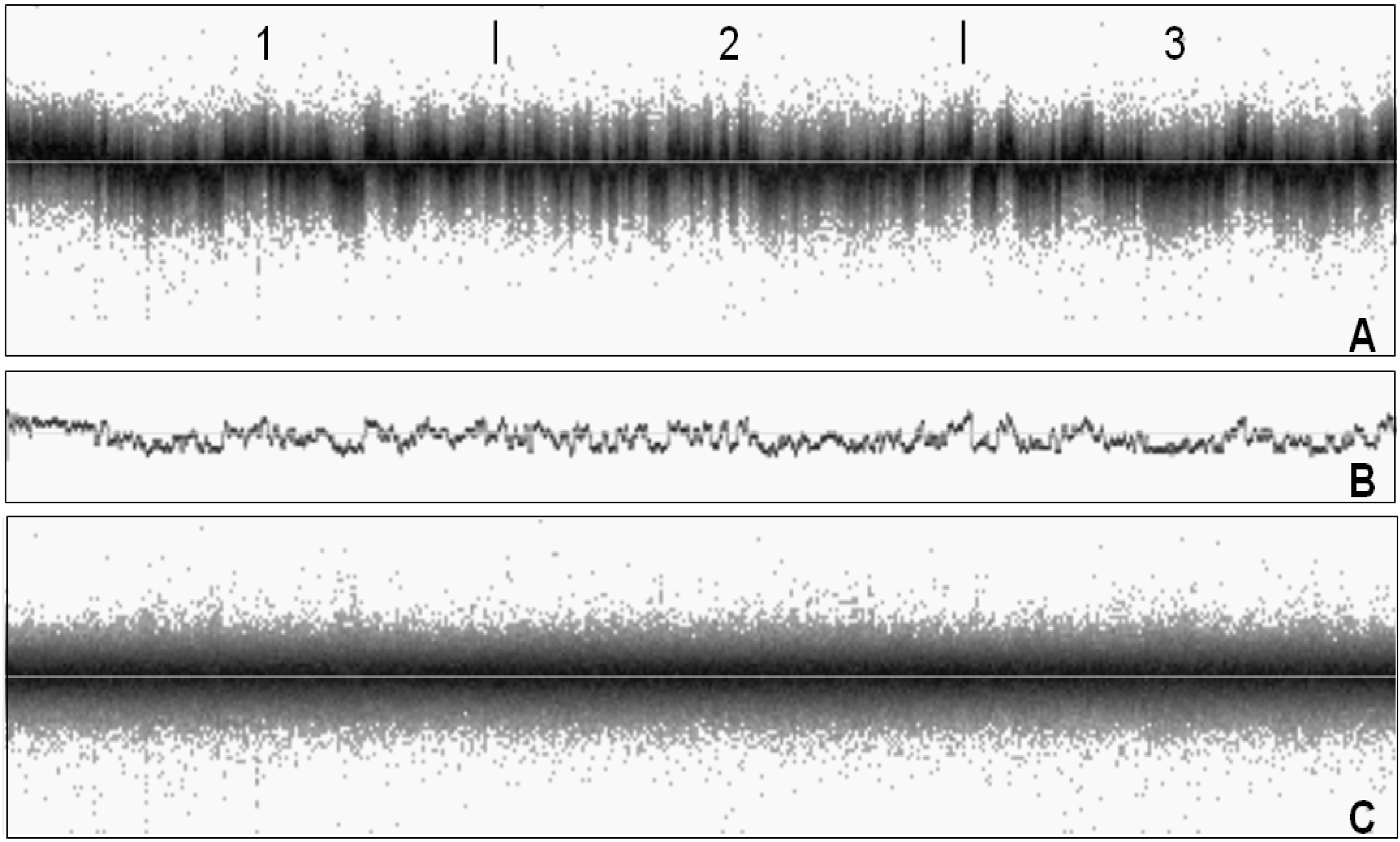
![Microarrays 02 00284 i001]() The same procedure is repeated on the per-SNP components.
The same procedure is repeated on the per-SNP components. - (3)
- Finally, the corrected components are added together and yield the corrected Log R Ratio values.

A3. Program Usage
| ID | call rate | var. | wave var. | per_SNP var. | Chr1 | Chr2 | Chr3 | Chr4 | Chr5 | Chr6 | Chr7 | Chr8 | Chr9 | Chr10 | Chr11 | Chr12 | Chr13 | Chr14 | Chr15 | Chr16 | Chr17 | Chr18 | Chr19 | Chr20 | Chr21 | Chr22 |
|---|---|---|---|---|---|---|---|---|---|---|---|---|---|---|---|---|---|---|---|---|---|---|---|---|---|---|
| 3 | 98.33 | 0.068 | 0.001 | 0.067 | 2 | 0 | 0 | 2 | 2 | 0 | 0 | 0 | 0 | 0 | 0 | 11 | 0 | 1 | 0 | 0 | 2 | 2 | 0 | 0 | 0 | 102 |
| 15 | 96.02 | 0.144 | 0.001 | 0.142 | 10 | 4 | 38 | 8 | 11 | 2 | 0 | 50 | 16 | 11 | 8 | 150 | 13 | 0 | 78 | 22 | 11 | 21 | 19 | 0 | 4 | 0 |
| 36 | 96.00 | 0.243 | 0.004 | 0.238 | 506 | 845 | 678 | 751 | 1,376 | 503 | 977 | 974 | 722 | 385 | 379 | 639 | 593 | 232 | 541 | 752 | 356 | 397 | 364 | 225 | 262 | 203 |
| 38 | 95.76 | 0.183 | 0.001 | 0.181 | 179 | 80 | 102 | 48 | 140 | 80 | 91 | 268 | 33 | 84 | 122 | 44 | 27 | 144 | 20 | 47 | 114 | 41 | 155 | 0 | 40 | 20 |
| 48 | 96.16 | 0.174 | 0.007 | 0.167 | 0 | 39 | 60 | 141 | 23 | 42 | 90 | 69 | 56 | 5 | 10 | 59 | 110 | 18 | 32 | 361 | 29 | 32 | 0 | 94 | 15 | 55 |
| 49 | 94.81 | 0.174 | 0.007 | 0.167 | 203 | 31 | 35 | 111 | 40 | 28 | 33 | 22 | 14 | 6 | 22 | 9 | 8 | 15 | 41 | 0 | 0 | 23 | 12 | 0 | 7 | 0 |
| 50 | 97.14 | 0.103 | 0.002 | 0.101 | 46 | 11 | 0 | 14 | 22 | 242 | 2 | 0 | 8 | 0 | 0 | 65 | 0 | 0 | 11 | 2 | 3 | 0 | 45 | 0 | 2 | 2 |
| 62 | 97.92 | 0.090 | 0.003 | 0.087 | 0 | 14 | 0 | 14 | 3 | 19 | 15 | 11 | 2 | 2 | 0 | 0 | 0 | 0 | 0 | 0 | 6 | 16 | 0 | 0 | 0 | 2 |
| 71 | 93.92 | 0.202 | 0.002 | 0.200 | 667 | 490 | 326 | 78 | 149 | 40 | 269 | 252 | 215 | 116 | 45 | 231 | 96 | 163 | 142 | 266 | 134 | 148 | 248 | 38 | 97 | 50 |
| 76 | 93.71 | 0.229 | 0.002 | 0.226 | 511 | 251 | 200 | 65 | 229 | 59 | 336 | 467 | 352 | 422 | 457 | 233 | 85 | 185 | 170 | 252 | 285 | 161 | 462 | 112 | 167 | 49 |
| 97 | 89.52 | 0.291 | 0.008 | 0.282 | 3,123 | 5,467 | 11,613 | 3,795 | 6,729 | 4,870 | 5,374 | 4,898 | 4,455 | 4,169 | 5,721 | 6,492 | 3,486 | 3,020 | 3,709 | 4,031 | 4,120 | 3,177 | 3,581 | 2,466 | 1,775 | 1,281 |
| 101 | 97.85 | 0.077 | 0.002 | 0.075 | 0 | 0 | 0 | 0 | 0 | 0 | 0 | 0 | 0 | 0 | 0 | 0 | 0 | 9 | 0 | 0 | 0 | 0 | 0 | 2 | 0 | 0 |
| 111 | 96.51 | 0.175 | 0.003 | 0.172 | 70 | 76 | 14 | 49 | 287 | 187 | 29 | 76 | 64 | 266 | 105 | 47 | 61 | 17 | 15 | 20 | 0 | 74 | 10 | 136 | 6 | 21 |
| 112 | 94.70 | 0.147 | 0.011 | 0.134 | 2,378 | 2,988 | 2,743 | 2,514 | 2,823 | 4,455 | 2,774 | 3,014 | 2,837 | 2,707 | 4,227 | 3,054 | 2,315 | 1,595 | 1,905 | 1,087 | 2,085 | 2,044 | 1,562 | 650 | 580 | 602 |
| 129 | 96.61 | 0.139 | 0.003 | 0.135 | 7 | 31 | 51 | 9 | 19 | 35 | 3 | 94 | 30 | 77 | 23 | 2 | 3 | 10 | 0 | 96 | 0 | 2 | 74 | 0 | 22 | 0 |
| 131 | 96.45 | 0.199 | 0.002 | 0.196 | 319 | 229 | 139 | 314 | 108 | 125 | 248 | 304 | 172 | 363 | 279 | 68 | 96 | 93 | 118 | 212 | 182 | 71 | 83 | 28 | 13 | 28 |
| 141 | 96.44 | 0.121 | 0.017 | 0.101 | 266 | 121 | 174 | 173 | 147 | 64 | 195 | 121 | 258 | 24 | 43 | 291 | 45 | 36 | 59 | 202 | 105 | 96 | 208 | 90 | 86 | 72 |
| 144 | 94.72 | 0.176 | 0.005 | 0.170 | 251 | 746 | 130 | 464 | 250 | 328 | 253 | 410 | 390 | 139 | 799 | 55 | 553 | 63 | 193 | 178 | 52 | 286 | 195 | 9 | 15 | 45 |
| 168 | 94.36 | 0.315 | 0.036 | 0.275 | 5,205 | 5,382 | 5,272 | 4,479 | 4,337 | 5,737 | 6,682 | 4,504 | 3,966 | 2,627 | 2,901 | 5,294 | 2,492 | 3,065 | 2,487 | 3,126 | 2,559 | 2,658 | 2,179 | 1,405 | 961 | 948 |
| 182 | 95.02 | 0.316 | 0.002 | 0.313 | 1,189 | 1,988 | 2,051 | 1,096 | 2,301 | 2,991 | 1,814 | 2,365 | 1,408 | 687 | 1,144 | 1,314 | 839 | 654 | 689 | 815 | 569 | 1,953 | 427 | 517 | 456 | 377 |
| 188 | 90.12 | 0.474 | 0.011 | 0.461 | 14,534 | 15,554 | 28,322 | 10,245 | 10,904 | 16,212 | 12,471 | 14,300 | 6,642 | 6,499 | 8,681 | 9,241 | 5,595 | 6,784 | 7,503 | 5,150 | 6,048 | 7,028 | 3,978 | 2,417 | 3,536 | 2,274 |
| 189 | 97.32 | 0.097 | 0.012 | 0.084 | 120 | 34 | 155 | 12 | 35 | 41 | 74 | 69 | 0 | 29 | 47 | 34 | 16 | 6 | 1 | 0 | 0 | 0 | 30 | 0 | 35 | 2 |
| 193 | 97.34 | 0.093 | 0.004 | 0.088 | 53 | 3 | 0 | 3 | 0 | 0 | 0 | 5 | 71 | 6 | 2 | 0 | 47 | 0 | 0 | 0 | 0 | 0 | 0 | 0 | 0 | 0 |
| 412 | 97.51 | 0.092 | 0.006 | 0.086 | 0 | 0 | 62 | 2 | 0 | 0 | 20 | 0 | 2 | 14 | 0 | 10 | 22 | 0 | 0 | 0 | 2 | 2 | 0 | 0 | 0 | 4 |
| 415 | 98.23 | 0.103 | 0.001 | 0.102 | 5 | 11 | 0 | 5 | 3 | 10 | 35 | 0 | 2 | 0 | 0 | 2 | 0 | 0 | 0 | 0 | 0 | 9 | 0 | 0 | 0 | 2 |
| 421 | 96.73 | 0.165 | 0.055 | 0.102 | 0 | 7 | 0 | 0 | 0 | 5 | 28 | 0 | 0 | 0 | 0 | 0 | 0 | 2 | 0 | 0 | 0 | 4 | 0 | 0 | 0 | 0 |
| 422 | 96.10 | 0.074 | 0.002 | 0.073 | 37,996 | 36,654 | 32,343 | 29,935 | 29,248 | 29,062 | 23,198 | 24,951 | 21,457 | 22,172 | 22,247 | 21,574 | 15,560 | 14,542 | 14,525 | 12,574 | 10,444 | 14,095 | 8,616 | 10,294 | 7,218 | 4,456 |
| 430 | 96.39 | 0.160 | 0.019 | 0.138 | 10,614 | 10,096 | 9,196 | 16,278 | 15,383 | 7,959 | 7,758 | 9,465 | 6,757 | 6,295 | 6,291 | 6,559 | 4,955 | 3,487 | 2,491 | 3,459 | 3,074 | 5,404 | 1,525 | 2,399 | 3,569 | 1,187 |
| 438 | 89.76 | 0.463 | 0.057 | 0.399 | 45,981 | 56,162 | 42,403 | 45,750 | 55,976 | 37,901 | 44,212 | 34,069 | 30,387 | 26,842 | 26,461 | 38,930 | 23,963 | 20,800 | 18,258 | 19,160 | 16,624 | 18,367 | 9,637 | 13,485 | 8,790 | 5,479 |
| 442 | 97.82 | 0.084 | 0.008 | 0.076 | 486 | 382 | 0 | 0 | 14 | 0 | 9 | 57 | 2 | 0 | 33 | 4 | 0 | 0 | 0 | 0 | 0 | 0 | 67 | 0 | 4 | 3 |
| 451 | 95.96 | 0.205 | 0.004 | 0.200 | 109 | 154 | 49 | 363 | 75 | 361 | 107 | 213 | 124 | 100 | 85 | 150 | 124 | 20 | 63 | 4 | 60 | 116 | 50 | 59 | 0 | 19 |
| 461 | 80.86 | 0.706 | 0.007 | 0.696 | 64,822 | 74,302 | 41,655 | 64,993 | 56,987 | 58,825 | 49,369 | 55,433 | 45,357 | 47,372 | 35,753 | 49,377 | 30,870 | 27,158 | 25,448 | 29,590 | 14,637 | 22,231 | 15,372 | 19,289 | 12,431 | 8,971 |
| 613 | 97.64 | 0.090 | 0.001 | 0.088 | 2 | 6 | 3 | 7 | 4 | 0 | 49 | 15 | 0 | 0 | 22 | 2 | 10 | 2 | 0 | 0 | 0 | 0 | 7 | 0 | 2 | 0 |
| 647 | 95.49 | 0.157 | 0.002 | 0.154 | 15 | 1 | 30 | 166 | 0 | 47 | 9 | 0 | 6 | 45 | 41 | 58 | 0 | 5 | 28 | 41 | 24 | 0 | 14 | 4 | 4 | 11 |
| 653 | 98.22 | 0.079 | 0.004 | 0.074 | 12 | 2 | 14 | 1,618 | 26 | 7 | 12 | 7 | 0 | 9 | 0 | 0 | 0 | 0 | 0 | 2 | 0 | 0 | 0 | 0 | 4 | 4 |
| 665 | 97.32 | 0.123 | 0.037 | 0.082 | 5,071 | 8,140 | 6,289 | 5,520 | 6,417 | 6,816 | 5,890 | 6,894 | 4,238 | 5,326 | 4,503 | 5,246 | 2,641 | 2,696 | 2,301 | 1,766 | 1,445 | 4,211 | 1,699 | 1,399 | 2,448 | 932 |
| 670 | 96.74 | 0.152 | 0.043 | 0.105 | 3,160 | 4,486 | 3,895 | 3,913 | 3,812 | 3,038 | 3,309 | 3,676 | 2,359 | 2,112 | 3,327 | 2,791 | 1,591 | 1,595 | 1,142 | 969 | 1,028 | 2,043 | 543 | 1,213 | 1,034 | 286 |
| 675 | 97.67 | 0.084 | 0.009 | 0.074 | 0 | 0 | 3 | 0 | 4 | 1 | 3 | 37 | 0 | 0 | 58 | 4 | 0 | 0 | 0 | 11 | 0 | 0 | 48 | 0 | 0 | 0 |
| 676 | 98.15 | 0.078 | 0.001 | 0.077 | 0 | 0 | 0 | 0 | 45 | 2 | 18 | 0 | 0 | 0 | 14 | 4 | 0 | 0 | 0 | 0 | 0 | 0 | 0 | 0 | 0 | 0 |
| 677 | 95.58 | 0.208 | 0.003 | 0.204 | 25 | 149 | 161 | 54 | 77 | 57 | 267 | 157 | 38 | 210 | 63 | 13 | 52 | 64 | 34 | 44 | 57 | 137 | 121 | 16 | 56 | 75 |
| 693 | 95.72 | 0.133 | 0.005 | 0.128 | 4 | 73 | 18 | 6 | 31 | 12 | 15 | 27 | 7 | 0 | 10 | 8 | 73 | 14 | 10 | 0 | 5 | 3 | 20 | 2 | 0 | 12 |
| 715 | 97.44 | 0.095 | 0.006 | 0.089 | 3 | 5 | 0 | 0 | 4 | 0 | 471 | 0 | 2 | 0 | 0 | 0 | 0 | 4 | 0 | 4 | 0 | 24 | 0 | 4 | 0 | 0 |
| 717 | 96.60 | 0.134 | 0.001 | 0.132 | 0 | 2 | 22 | 21 | 29 | 41 | 0 | 17 | 0 | 6 | 57 | 10 | 0 | 2 | 0 | 15 | 0 | 0 | 34 | 0 | 0 | 0 |
| 729 | 94.75 | 0.189 | 0.001 | 0.187 | 115 | 23 | 115 | 184 | 49 | 55 | 84 | 91 | 42 | 45 | 101 | 111 | 16 | 57 | 103 | 80 | 57 | 61 | 192 | 0 | 22 | 0 |
| 733 | 95.84 | 0.198 | 0.009 | 0.188 | 23 | 28 | 84 | 218 | 218 | 0 | 306 | 180 | 40 | 34 | 59 | 11 | 32 | 3 | 33 | 62 | 108 | 6 | 8 | 38 | 46 | 0 |
| 735 | 95.28 | 0.173 | 0.003 | 0.169 | 94 | 21 | 111 | 290 | 81 | 41 | 116 | 14 | 220 | 79 | 0 | 87 | 47 | 31 | 34 | 43 | 16 | 13 | 181 | 0 | 0 | 22 |
| 742 | 96.83 | 0.114 | 0.013 | 0.099 | 0 | 0 | 3 | 0 | 2 | 0 | 1 | 0 | 4 | 0 | 2 | 0 | 0 | 15 | 8 | 2 | 18 | 0 | 137 | 0 | 0 | 0 |
| 744 | 97.26 | 0.108 | 0.017 | 0.089 | 0 | 135 | 126 | 332 | 73 | 148 | 263 | 0 | 135 | 31 | 52 | 150 | 180 | 34 | 15 | 40 | 0 | 166 | 114 | 0 | 94 | 0 |
| 746 | 95.72 | 0.253 | 0.004 | 0.248 | 283 | 895 | 350 | 378 | 287 | 388 | 227 | 723 | 594 | 712 | 229 | 559 | 323 | 206 | 98 | 478 | 398 | 689 | 341 | 73 | 184 | 173 |
| 750 | 97.15 | 0.114 | 0.015 | 0.097 | 2,389 | 642 | 1,750 | 1,501 | 1,370 | 1,792 | 707 | 1,440 | 997 | 615 | 674 | 750 | 559 | 225 | 544 | 63 | 187 | 814 | 458 | 177 | 184 | 0 |
| 752 | 97.80 | 0.103 | 0.004 | 0.099 | 88 | 121 | 119 | 155 | 196 | 83 | 118 | 187 | 93 | 206 | 66 | 147 | 27 | 35 | 50 | 41 | 32 | 70 | 15 | 36 | 27 | 25 |
| 796 | 94.23 | 0.247 | 0.002 | 0.244 | 2,165 | 482 | 568 | 1,127 | 539 | 263 | 360 | 591 | 440 | 697 | 908 | 806 | 106 | 630 | 256 | 498 | 262 | 565 | 127 | 275 | 67 | 48 |
| 1020 | 98.21 | 0.075 | 0.001 | 0.074 | 2 | 0 | 0 | 0 | 2 | 1 | 2 | 0 | 0 | 0 | 0 | 3 | 0 | 0 | 0 | 0 | 0 | 0 | 8 | 0 | 16 | 0 |
| 1022 | 97.77 | 0.082 | 0.001 | 0.081 | 6 | 16 | 2 | 30 | 2 | 2 | 2 | 0 | 12 | 0 | 11 | 0 | 0 | 0 | 0 | 0 | 0 | 1 | 0 | 0 | 0 | 0 |
| 1026 | 98.34 | 0.066 | 0.001 | 0.064 | 1 | 0 | 0 | 0 | 5 | 0 | 0 | 0 | 0 | 0 | 2 | 0 | 0 | 11 | 9 | 0 | 0 | 0 | 3 | 0 | 0 | 0 |
| 1028 | 97.49 | 0.089 | 0.001 | 0.088 | 9 | 0 | 0 | 0 | 40 | 49 | 0 | 3 | 0 | 0 | 3 | 0 | 0 | 0 | 0 | 0 | 0 | 0 | 0 | 0 | 0 | 0 |
| 1029 | 98.54 | 0.062 | 0.001 | 0.060 | 3 | 64 | 0 | 0 | 0 | 0 | 0 | 0 | 0 | 0 | 1 | 0 | 2 | 50 | 0 | 25 | 0 | 2 | 0 | 0 | 0 | 0 |
| 1033 | 97.58 | 0.087 | 0.001 | 0.085 | 0 | 0 | 83 | 0 | 0 | 0 | 2 | 0 | 70 | 4 | 4 | 0 | 0 | 0 | 8 | 0 | 0 | 0 | 0 | 0 | 0 | 0 |
| 1034 | 97.50 | 0.092 | 0.010 | 0.081 | 0 | 0 | 0 | 2 | 0 | 0 | 1 | 2 | 0 | 0 | 0 | 0 | 0 | 0 | 0 | 0 | 0 | 0 | 0 | 0 | 0 | 0 |
| 1037 | 98.26 | 0.068 | 0.001 | 0.067 | 8 | 5 | 2 | 50 | 2 | 6 | 2 | 12 | 0 | 2 | 1 | 0 | 2 | 0 | 0 | 3 | 54 | 13 | 2 | 2 | 0 | 0 |
| 1040 | 96.56 | 0.114 | 0.001 | 0.113 | 9 | 0 | 17 | 53 | 3 | 1 | 4 | 0 | 0 | 0 | 0 | 0 | 17 | 0 | 0 | 0 | 0 | 0 | 0 | 0 | 1 | 0 |
| 1041 | 97.16 | 0.094 | 0.001 | 0.093 | 0 | 0 | 0 | 4 | 2 | 2 | 0 | 0 | 0 | 0 | 13 | 3 | 0 | 0 | 0 | 0 | 0 | 0 | 0 | 0 | 0 | 0 |
| 1042 | 97.46 | 0.087 | 0.003 | 0.084 | 15 | 14 | 19 | 20 | 11 | 28 | 10 | 19 | 4 | 2 | 2 | 6 | 8 | 4 | 18 | 4 | 2 | 24 | 2 | 0 | 2 | 0 |
| 1056 | 97.11 | 0.098 | 0.003 | 0.095 | 2 | 0 | 2 | 2 | 0 | 2 | 0 | 0 | 0 | 0 | 0 | 15 | 0 | 4 | 0 | 0 | 35 | 0 | 10 | 0 | 0 | 18 |
| 1063 | 98.31 | 0.075 | 0.002 | 0.072 | 0 | 2 | 169 | 10 | 0 | 0 | 29 | 0 | 0 | 0 | 0 | 0 | 2 | 0 | 13 | 0 | 0 | 0 | 2 | 0 | 0 | 0 |
| 1065 | 98.23 | 0.068 | 0.003 | 0.065 | 0 | 4 | 2 | 7 | 0 | 0 | 0 | 2 | 0 | 0 | 0 | 0 | 8 | 0 | 0 | 0 | 0 | 58 | 4 | 0 | 0 | 0 |
| 1088 | 97.64 | 0.092 | 0.004 | 0.088 | 53 | 23 | 61 | 45 | 8 | 90 | 26 | 76 | 32 | 44 | 50 | 71 | 34 | 6 | 15 | 54 | 0 | 22 | 13 | 4 | 9 | 39 |
| 1091 | 96.69 | 0.138 | 0.029 | 0.105 | 7,631 | 6,080 | 7,146 | 6,512 | 7,299 | 4,006 | 4,952 | 6,666 | 4,169 | 2,579 | 3,990 | 4,012 | 2,388 | 2,194 | 1,415 | 2,613 | 1,030 | 2,828 | 646 | 3,697 | 1,862 | 451 |
| 1147 | 97.96 | 0.079 | 0.002 | 0.077 | 5 | 76 | 4 | 8 | 0 | 0 | 4 | 4 | 16 | 0 | 2 | 3 | 2 | 0 | 2 | 2 | 0 | 7 | 190 | 0 | 0 | 0 |
| 1151 | 97.90 | 0.087 | 0.001 | 0.086 | 2 | 4 | 0 | 0 | 3 | 0 | 0 | 8 | 0 | 4 | 9 | 0 | 0 | 0 | 0 | 0 | 2 | 0 | 0 | 0 | 11 | 2 |
| 2110 | 93.16 | 0.343 | 0.010 | 0.332 | 671 | 3,307 | 3,614 | 1,414 | 3,548 | 3,035 | 2,775 | 2,070 | 1,581 | 2,718 | 2,153 | 2,054 | 1,573 | 1,426 | 995 | 1,173 | 1,584 | 1,358 | 662 | 285 | 971 | 581 |
| 2134 | 95.73 | 0.134 | 0.008 | 0.125 | 144 | 52 | 81 | 51 | 51 | 100 | 28 | 88 | 70 | 0 | 35 | 77 | 3 | 55 | 7 | 16 | 56 | 7 | 41 | 2 | 18 | 1 |
| 2144 | 97.12 | 0.093 | 0.004 | 0.089 | 2 | 5 | 8 | 1 | 4 | 0 | 4 | 0 | 2 | 0 | 14 | 4 | 0 | 0 | 0 | 3 | 0 | 0 | 0 | 2 | 0 | 0 |
| 2240 | 94.48 | 0.299 | 0.004 | 0.294 | 488 | 1,656 | 1,019 | 1,734 | 2,180 | 1,605 | 754 | 1,750 | 1,179 | 531 | 916 | 1,728 | 916 | 751 | 643 | 921 | 501 | 427 | 713 | 356 | 339 | 374 |
| 2355 | 94.50 | 0.258 | 0.026 | 0.229 | 1,870 | 1,799 | 1,422 | 741 | 1,491 | 2,829 | 1,663 | 1,353 | 829 | 1,500 | 1,360 | 1,714 | 654 | 677 | 1,262 | 767 | 1,420 | 1,061 | 842 | 826 | 464 | 452 |
| 2406 | 94.78 | 0.195 | 0.011 | 0.183 | 67 | 125 | 136 | 122 | 201 | 80 | 142 | 109 | 62 | 61 | 5 | 51 | 70 | 68 | 34 | 7 | 60 | 83 | 122 | 53 | 43 | 0 |
| D_062 | 94.17 | 0.322 | 0.003 | 0.318 | 772 | 838 | 547 | 536 | 4,419 | 436 | 711 | 496 | 239 | 308 | 219 | 582 | 319 | 215 | 222 | 81 | 62 | 540 | 101 | 86 | 0 | 94 |
| ID | variance | wave variance | per-SNP variance | wave correlation | per-SNP correlation | wave subtraction factor | per-SNP subtraction factor |
|---|---|---|---|---|---|---|---|
| 3 | 0.068 | 0.001 | 0.067 | 0.804 | 0.676 | 0.409 | 0.800 |
| 15 | 0.144 | 0.001 | 0.142 | 0.567 | 0.564 | 0.393 | 0.972 |
| 36 | 0.243 | 0.004 | 0.238 | 0.877 | 0.388 | 0.997 | 0.865 |
| 38 | 0.183 | 0.001 | 0.181 | 0.456 | 0.502 | 0.314 | 0.977 |
| 48 | 0.174 | 0.007 | 0.167 | 0.939 | 0.508 | 1.405 | 0.949 |
| 49 | 0.174 | 0.007 | 0.167 | 0.959 | 0.527 | 1.419 | 0.985 |
| 50 | 0.103 | 0.002 | 0.101 | 0.881 | 0.536 | 0.626 | 0.779 |
| 62 | 0.090 | 0.003 | 0.087 | 0.929 | 0.609 | 0.886 | 0.820 |
| 71 | 0.202 | 0.002 | 0.200 | 0.365 | 0.589 | 0.274 | 1.203 |
| 76 | 0.229 | 0.002 | 0.226 | 0.580 | 0.529 | 0.511 | 1.151 |
| 97 | 0.291 | 0.008 | 0.282 | 0.875 | 0.360 | 1.427 | 0.873 |
| 101 | 0.077 | 0.002 | 0.075 | 0.906 | 0.727 | 0.717 | 0.910 |
| 111 | 0.175 | 0.003 | 0.172 | 0.914 | 0.482 | 0.903 | 0.914 |
| 112 | 0.147 | 0.011 | 0.134 | 0.864 | 0.578 | 1.671 | 0.968 |
| 129 | 0.139 | 0.003 | 0.135 | 0.898 | 0.620 | 0.964 | 1.043 |
| 131 | 0.199 | 0.002 | 0.196 | 0.875 | 0.417 | 0.790 | 0.844 |
| 141 | 0.121 | 0.017 | 0.101 | 0.949 | 0.703 | 2.297 | 1.024 |
| 144 | 0.176 | 0.005 | 0.170 | 0.881 | 0.591 | 1.141 | 1.115 |
| 168 | 0.315 | 0.036 | 0.275 | 0.936 | 0.406 | 3.234 | 0.975 |
| 182 | 0.316 | 0.002 | 0.313 | 0.809 | 0.386 | 0.704 | 0.990 |
| 189 | 0.097 | 0.012 | 0.084 | 0.930 | 0.668 | 1.874 | 0.883 |
| 193 | 0.093 | 0.004 | 0.088 | 0.960 | 0.704 | 1.174 | 0.956 |
| 412 | 0.092 | 0.006 | 0.086 | 0.950 | 0.691 | 1.304 | 0.925 |
| 421 | 0.103 | 0.001 | 0.102 | 0.898 | 0.680 | 0.598 | 0.991 |
| 422 | 0.165 | 0.055 | 0.102 | 0.873 | 0.523 | 3.763 | 0.763 |
| 425 | 0.074 | 0.002 | 0.073 | 0.908 | 0.572 | 0.653 | 0.705 |
| 430 | 0.160 | 0.019 | 0.138 | 0.896 | 0.457 | 2.265 | 0.778 |
| 438 | 0.463 | 0.057 | 0.399 | 0.913 | 0.354 | 4.006 | 1.021 |
| 442 | 0.084 | 0.008 | 0.076 | 0.942 | 0.663 | 1.496 | 0.835 |
| 451 | 0.205 | 0.004 | 0.200 | 0.927 | 0.453 | 1.111 | 0.927 |
| 461 | 0.706 | 0.007 | 0.696 | −0.310 | 0.228 | −0.460 | 0.868 |
| 613 | 0.090 | 0.001 | 0.088 | 0.850 | 0.565 | 0.589 | 0.767 |
| 647 | 0.157 | 0.002 | 0.154 | 0.766 | 0.589 | 0.671 | 1.059 |
| 653 | 0.079 | 0.004 | 0.074 | 0.938 | 0.569 | 1.141 | 0.707 |
| 665 | 0.123 | 0.037 | 0.082 | 0.896 | 0.555 | 3.159 | 0.726 |
| 670 | 0.152 | 0.043 | 0.105 | 0.906 | 0.565 | 3.422 | 0.837 |
| 675 | 0.084 | 0.009 | 0.074 | 0.951 | 0.672 | 1.647 | 0.837 |
| 676 | 0.078 | 0.001 | 0.077 | 0.646 | 0.635 | 0.313 | 0.807 |
| 677 | 0.208 | 0.003 | 0.204 | 0.901 | 0.465 | 0.870 | 0.960 |
| 693 | 0.133 | 0.005 | 0.128 | 0.953 | 0.581 | 1.179 | 0.952 |
| 715 | 0.095 | 0.006 | 0.089 | 0.950 | 0.667 | 1.308 | 0.911 |
| 717 | 0.134 | 0.001 | 0.132 | 0.522 | 0.650 | 0.351 | 1.081 |
| 729 | 0.189 | 0.001 | 0.187 | 0.606 | 0.611 | 0.411 | 1.209 |
| 733 | 0.198 | 0.009 | 0.188 | 0.947 | 0.488 | 1.628 | 0.967 |
| 735 | 0.173 | 0.003 | 0.169 | 0.901 | 0.609 | 0.917 | 1.144 |
| 742 | 0.114 | 0.013 | 0.099 | 0.956 | 0.649 | 2.017 | 0.936 |
| 744 | 0.108 | 0.017 | 0.089 | 0.921 | 0.570 | 2.186 | 0.779 |
| 746 | 0.253 | 0.004 | 0.248 | 0.906 | 0.414 | 1.033 | 0.943 |
| 750 | 0.114 | 0.015 | 0.097 | 0.940 | 0.612 | 2.137 | 0.874 |
| 752 | 0.103 | 0.004 | 0.099 | 0.937 | 0.471 | 1.033 | 0.679 |
| 796 | 0.247 | 0.002 | 0.244 | 0.015 | 0.527 | 0.012 | 1.192 |
| 1020 | 0.075 | 0.001 | 0.074 | 0.742 | 0.614 | 0.348 | 0.767 |
| 1022 | 0.082 | 0.001 | 0.081 | 0.909 | 0.644 | 0.640 | 0.836 |
| 1026 | 0.066 | 0.001 | 0.064 | 0.861 | 0.664 | 0.557 | 0.770 |
| 1028 | 0.089 | 0.001 | 0.088 | 0.742 | 0.643 | 0.380 | 0.871 |
| 1029 | 0.062 | 0.001 | 0.060 | 0.912 | 0.661 | 0.572 | 0.742 |
| 1033 | 0.087 | 0.001 | 0.085 | 0.820 | 0.703 | 0.518 | 0.940 |
| 1034 | 0.092 | 0.010 | 0.081 | 0.963 | 0.709 | 1.732 | 0.924 |
| 1037 | 0.068 | 0.001 | 0.067 | 0.782 | 0.633 | 0.390 | 0.748 |
| 1040 | 0.114 | 0.001 | 0.113 | 0.639 | 0.701 | 0.355 | 1.077 |
| 1041 | 0.094 | 0.001 | 0.093 | 0.850 | 0.672 | 0.546 | 0.937 |
| 1042 | 0.087 | 0.003 | 0.084 | 0.947 | 0.695 | 0.884 | 0.921 |
| 1056 | 0.098 | 0.003 | 0.095 | 0.941 | 0.686 | 0.893 | 0.966 |
| 1063 | 0.075 | 0.002 | 0.072 | 0.924 | 0.571 | 0.832 | 0.701 |
| 1065 | 0.068 | 0.003 | 0.065 | 0.959 | 0.657 | 0.904 | 0.764 |
| 1088 | 0.092 | 0.004 | 0.088 | 0.918 | 0.497 | 1.046 | 0.675 |
| 1091 | 0.138 | 0.029 | 0.105 | 0.912 | 0.537 | 2.854 | 0.797 |
| 1147 | 0.079 | 0.002 | 0.077 | 0.944 | 0.717 | 0.795 | 0.909 |
| 1151 | 0.087 | 0.001 | 0.086 | 0.688 | 0.572 | 0.311 | 0.769 |
| 2110 | 0.343 | 0.010 | 0.332 | 0.948 | 0.408 | 1.715 | 1.075 |
| 2134 | 0.134 | 0.008 | 0.125 | 0.936 | 0.551 | 1.575 | 0.893 |
| 2144 | 0.093 | 0.004 | 0.089 | 0.953 | 0.609 | 1.046 | 0.832 |
| 2240 | 0.299 | 0.004 | 0.294 | 0.909 | 0.433 | 1.060 | 1.075 |
| 2355 | 0.258 | 0.026 | 0.229 | 0.960 | 0.530 | 2.826 | 1.161 |
| 2406 | 0.195 | 0.011 | 0.183 | 0.940 | 0.570 | 1.833 | 1.113 |
| 188c | 0.474 | 0.011 | 0.461 | 0.899 | 0.314 | 1.715 | 0.975 |
| D62 | 0.322 | 0.003 | 0.318 | 0.819 | 0.340 | 0.761 | 0.878 |
© 2013 by the authors; licensee MDPI, Basel, Switzerland. This article is an open access article distributed under the terms and conditions of the Creative Commons Attribution license (http://creativecommons.org/licenses/by/3.0/).
Share and Cite
Ginsbach, P.; Chen, B.; Jiang, Y.; Engelter, S.T.; Grond-Ginsbach, C. Copy Number Studies in Noisy Samples. Microarrays 2013, 2, 284-303. https://doi.org/10.3390/microarrays2040284
Ginsbach P, Chen B, Jiang Y, Engelter ST, Grond-Ginsbach C. Copy Number Studies in Noisy Samples. Microarrays. 2013; 2(4):284-303. https://doi.org/10.3390/microarrays2040284
Chicago/Turabian StyleGinsbach, Philip, Bowang Chen, Yanxiang Jiang, Stefan T. Engelter, and Caspar Grond-Ginsbach. 2013. "Copy Number Studies in Noisy Samples" Microarrays 2, no. 4: 284-303. https://doi.org/10.3390/microarrays2040284