Development of a Vibroacoustic Stochastic Finite Element Prediction Tool for a CLT Floor


1
Department of Applied Sciences, University of Québec at Chicoutimi, Chicoutimi, QC G7H2B1, Canada
2
Division of Engineering Acoustics, Department of Construction Sciences, Lund University, 22362 Lund, Sweden
3
Saint-Gobain Ecophon Spain, 28020 Madrid, Spain
*
Author to whom correspondence should be addressed.
Appl. Sci. 2019, 9(6), 1106; https://doi.org/10.3390/app9061106
Submission received: 31 January 2019
/
Revised: 2 March 2019
/
Accepted: 8 March 2019
/
Published: 15 March 2019
(This article belongs to the Special Issue Modelling, Simulation and Data Analysis in Acoustical Problems)
Abstract
:Low frequency impact sound insulation is a challenging task in wooden buildings. Low frequency prediction tools are needed to access the dynamic behavior of a wooden floor in an early design phase to ultimately reduce the low frequency impact noise. However, due to the complexity of wood and different structural details, accurate vibration predictions of wood structures are difficult to attain. Meanwhile, a deterministic model cannot properly represent the real case due to the uncertainties coming from the material properties and geometrical changes. The stochastic approach introduced in this paper aims at quantifying the uncertainties induced by material properties and proposing an alternative calibration method to obtain a relative accurate result instead of the conventional manual calibration. In addition, 100 simulations were calculated in different excitation positions to assess the uncertainties induced by material properties of cross-laminated-timber A comparison between the simulated and measured results was made in order to extract the best combination of Young’s moduli and shear moduli in different directions of the CLT panel.
1. Introduction
Multi-story wooden constructions have increased in the market during the last two decades. However, this kind of constructions still face the challenge coming from low-frequency sound insulation. Although these types of buildings comply with the present regulations, subjective ratings of inhabitants have shown complaints [1,2,3,4,5,6] due to low-frequency impact noise. One of the important reasons resulting in this discrepancy between the subjective and objective evaluations is that the current standards are initially designed for heavy constructions, i.e., concrete constructions, but without an appropriate modification, they are directly applied to the wooden constructions. On the other hand, the low frequency impact noise is neglected in the standardized impact sound insulation evaluations. From recent research [3], it was shown that the subjective ratings are correlated better with the objective ratings with the help of the adaptation term following the standard ISO 717-2 [7]. But the correlation between the inhabitants’ satisfaction (reported by means of questionnaires) and objective ratings can be further improved by taking the measurement from 20 Hz in comparison with the measurements performed from 50 Hz instead. Furthermore, the dynamic behavior of wood (as a natural material) is hard to predict due to its inhomogeneity. As a consequence, product development in the wooden industry is still based on empirical models and experimental tests, which could lead to an over-designed and expensive acoustical improvement solution. To end that, more knowledge about wooden construction is needed and accurate and handy prediction tools are called for in order to enable acoustic comfort in wooden constructions, especially in a low-frequency range.
The finite element (FE) method is a widely employed approach to develop numerical prediction models in wooden industry. By performing numerical simulations, experimental acoustical tests can be reduced, and parametric studies can also be carried out to investigate the influence of specific geometrical changes in construction as well as the influence of the variations/uncertainties in material properties, which always have a markable influence on the results. In Reference [8], experimental tests were conducted on a full-scale cross-laminated timber (CLT) floor. The material properties of the CLT were collected from the literature and then put into the established FE model to compare the simulation results with the measured ones. A better correlation between the testing results and the modelling results was attained after tuning the collected material properties of CLT. The latter points out the importance of knowing the material properties if a proper calculation of dynamic properties needs to be achieved. A similar conclusion was drawn in References [9,10,11].
However, one should know that the variety of the wood species, the variation in theoretical identical wood structure, as well as the lack of material properties data base, make the reliable material properties of wood difficult to obtain. Consequently, the calibration of a model is always tedious and time-consuming. Moreover, even with the calibrated model to predict the theoretical identical wooden structure, the prediction results may be different from the realistic case due to the uncertainties induced by wooden material properties, workmanship and geometrical details in structures. As a result, the deterministic model may not be representative enough in a realistic situation. Therefore, it is a necessary step to quantify the variations in the model’s outputs in order to ultimately establish an accurate prediction tool. To achieve that, uncertainties of the wood material properties can be addressed in a model by introducing probabilistic parameters [6]. In Reference [12], a generalized probabilistic model was constructed to take into account the statistical fluctuation associated with the elastic properties in the model. The uncertainties of the mechanical constants of a wooden structure were also investigated in Reference [13]. A small data base of the Young’s modulus in the longitudinal direction was established by means of vibration measurements. Then, by sampling the Young’s modulus distribution established by the obtained data base, Monte Carlo simulations were performed in the FE model development to quantify the uncertainties induced by the elastic constants in modelling the vibro-acoustic behavior of wooden buildings in a low-frequency range. However, not only does the Young’s modulus in the longitudinal direction have a great impact on the dynamic response of a wooden structure, but the Young’s moduli in the other two directions as well as the shear moduli play an important role in its vibroacoustic performance. Regarding the uncertainties in structural dynamics, Shannon’s maximum entropy principle [14] is an optimal choice to model the random data and the uncertainties [15]. In Reference [16,17], a probabilistic model was proposed to construct the probability distribution in high-dimension of a vector-valued random variable using the maximum entropy principle. This proposed probabilistic model was then extended to a tensor-valued coefficient (stiffness tensor) with different symmetric levels [15,18,19].
The research reported in this case aims at developing a stochastic FE prediction tool of a CLT slab in order to quantify the uncertainties induced by material properties and, subsequently, acquire the reliable material properties of the under investigated structure to accurately predict the vibroacoustic behavior of CLT in a low-frequency range. To achieve that, different mechanical constant distributions without available material property data base are constructed by means of the maximum entropy principle. The random elastic constants generated following the established distributions are considered as the inputs for the FE model to calibrate CLT in a low frequency range by comparing the simulated results with its dynamic responses obtained from experimental modal analysis (EMA) method. The best combination of the material properties of CLT panel is selected by minimizing different error metrics. The ultimate objective is to acquire the knowledge about the modeling method of CLT and to propose a generalized method to quantify the uncertainties coming from the orthotropic level material properties and to accurately calibrate the corresponding model by avoiding the repetitive manual calibration and, subsequently, to increase the prediction accuracy.
2. Measurements
2.1. Experimental Structure
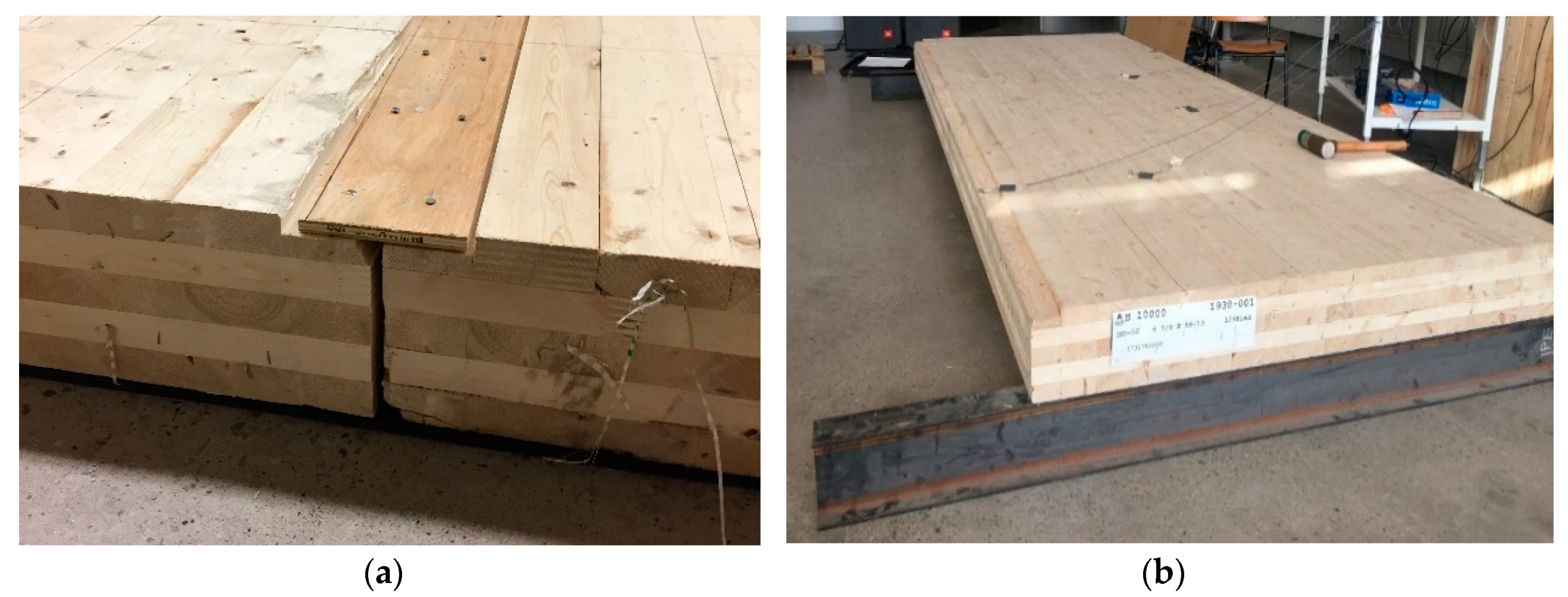
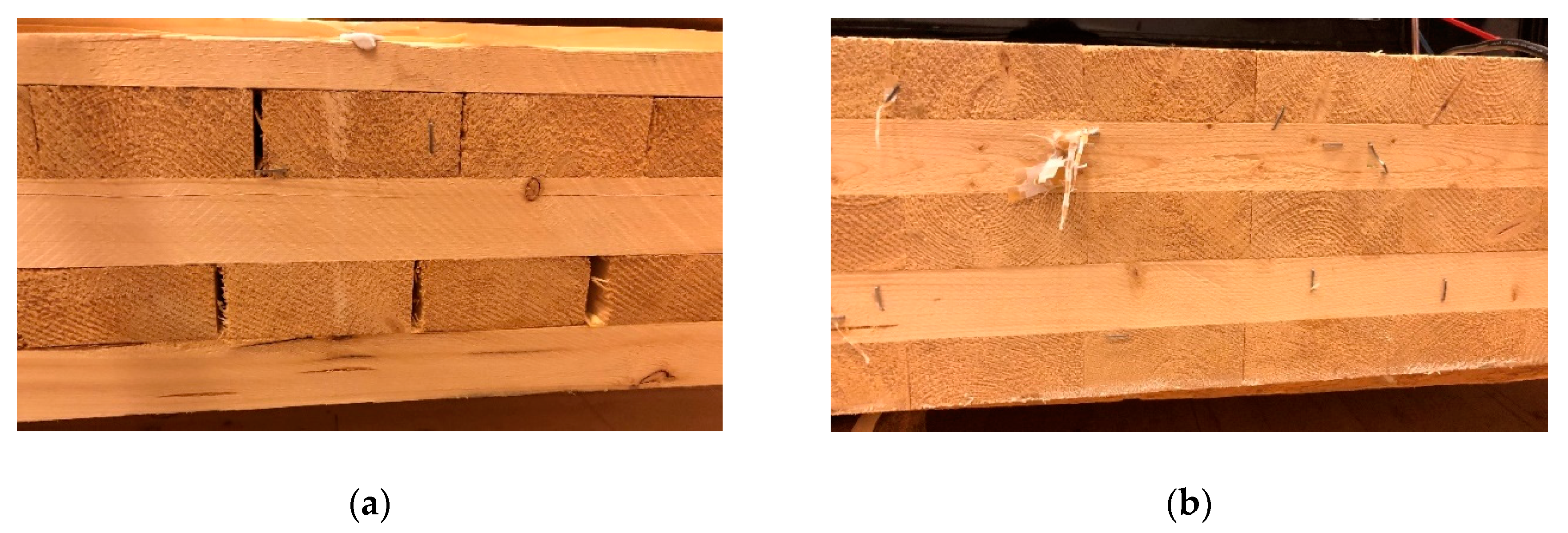
The test structure was a 4 × 1.5 m2 5-ply 175 mm thick CLT panel made of Canadian black spruce of machine stress rated grade 1950f-1.7E in parallel layers and visual grade No. 3 in perpendicular layers with density of 520 kg/m3. At the initial stage, two CLT slabs were nailed together by a thin wooden panel (c.f. Figure 1a) and they were placed on a standardized sound insulation measurement console. However, this weak connection between two CLT panels resulted in a low stiffness coupling between two slabs and the imperfect simply supported boundary conditions of the measurement console makes the CLT floor easily “jump up” when there is an external excitation. In a real building construction, these problems can be resolved by adding a top layer on the CLT bare floor, which can add mass on CLT and, subsequently, enforce the connection between two CLT leaves. Consequently, due to the weak connection between two assembled CLT panels and the imperfect boundary conditions in the sound insulation laboratory, only the first eigen-mode can be extracted from the measurements, which cannot provide enough information to calibrate the established FE model. As a result, in order to easily extract more meaningful information, only one leaf of CLT floor was under investigation.
2.2. Measurement Procedure
2.2.1. Measurement Setup
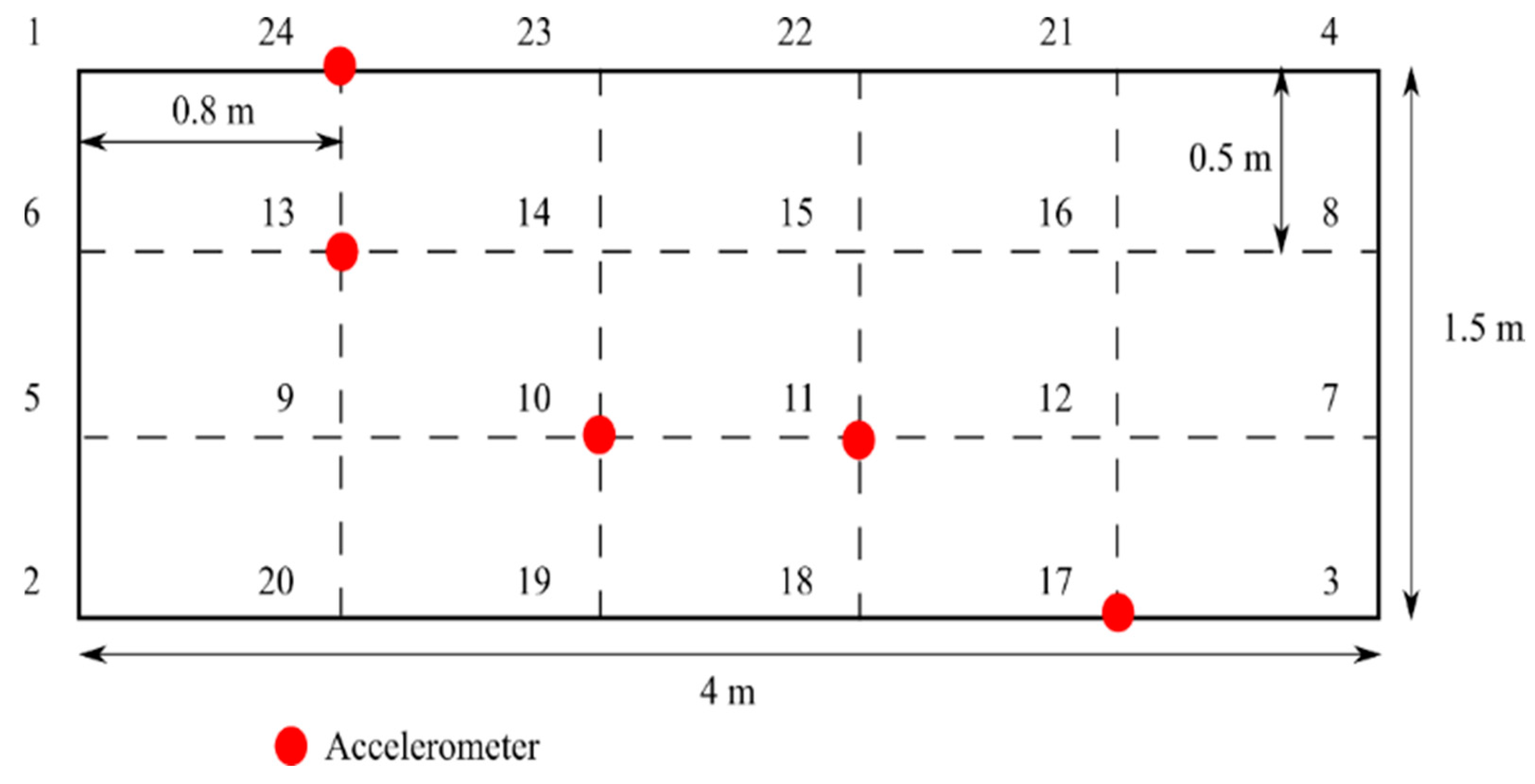
EMA was performed on the CLT slab to characterize the dynamic properties of the CLT slab. The CLT panel was set free at two opposite long sides and simply supported (SFSF boundary condition) with two steel I-beams at two shorter edges (shown in Figure 1b) in order to simplify the boundary conditions. A predefined mesh was drawn on the CLT surface to determine the excitation positions and the measurement positions. In that way, the CLT was divided into five parts in the long direction and three parts in the short direction, which gives a total number of 16 excitation points (the nodes on the short edges were not excited). The size of mesh was decided based upon the highest frequency of interest, i.e., 200 Hz, to avoid the hammer exciting on the nodes of the eigen-modes.
A single input multiple output system (SIMO) can provide redundant data to better identify the eigen-frequencies and the local modes of complex structures based on different frequency response function (FRF) matrices [20,21]. Meanwhile, these different FRFs can be used as references to validate the FE model by comparing different simulated FRFs with different measured FRFs. Concerning the complexity and the inhomogeneity of CLT, the SIMO system was employed to characterize the dynamic properties of the CLT panel via different FRF matrices at different measurement positions. Five uni-axial accelerometers (Brüel & Kjær Accelerometer Type 4507 001, Brüel & Kjær Sound & Vibration Measurement A/S, Nærum, Denmark) were attached on the different nodes (red dots in Figure 2) with the help of Faber-Castell Tack-It Multipurpose Adhesive. An impact roving hammer (Brüel & Kjær Impact hammer Type 8208 serial No. 51994, Brüel & Kjær Sound & Vibration Measurement A/S, Nærum, Denmark) was used as excitation.
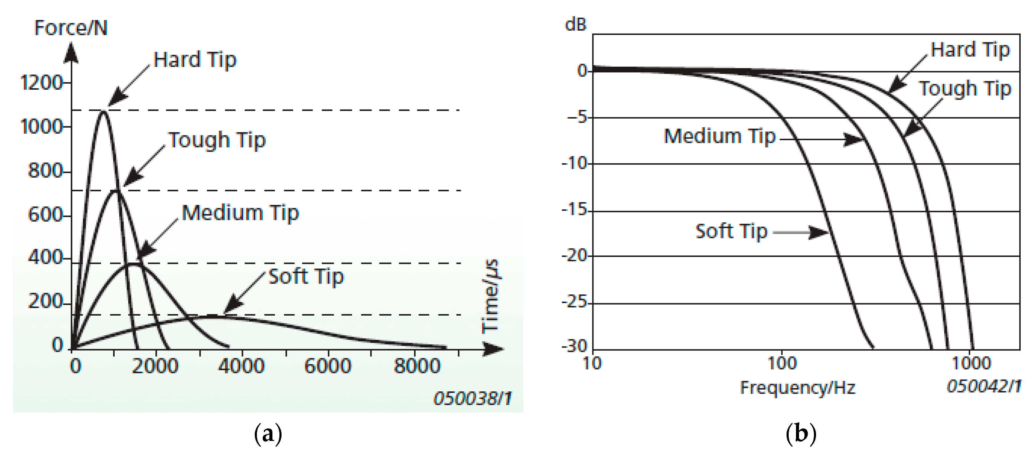
Depending on the impulse shape and the force spectrum of the impact hammer shown in Figure 3, the medium hard hammer tip was selected for this measurement to ensure most of the input energy localizing within the frequency range of interest (up to 200 Hz). The roving hammer approach was employed. The accelerometers were kept fixing on the selected positions and the hammer were roved over the predefined mesh grid except for the points on boundaries. The accelerometers and the impact hammer were connected to Brüel & Kjær multi-channel front-end LAN-XI Type 3050. Then, the acceleration signals and the impact force signals were recorded by using the software Brüel & Kjær PULSE Labshop. There were three averages for each excitation position. The resolution of the FRF was 0.625 Hz.
2.2.2. Modal Parameters Extraction
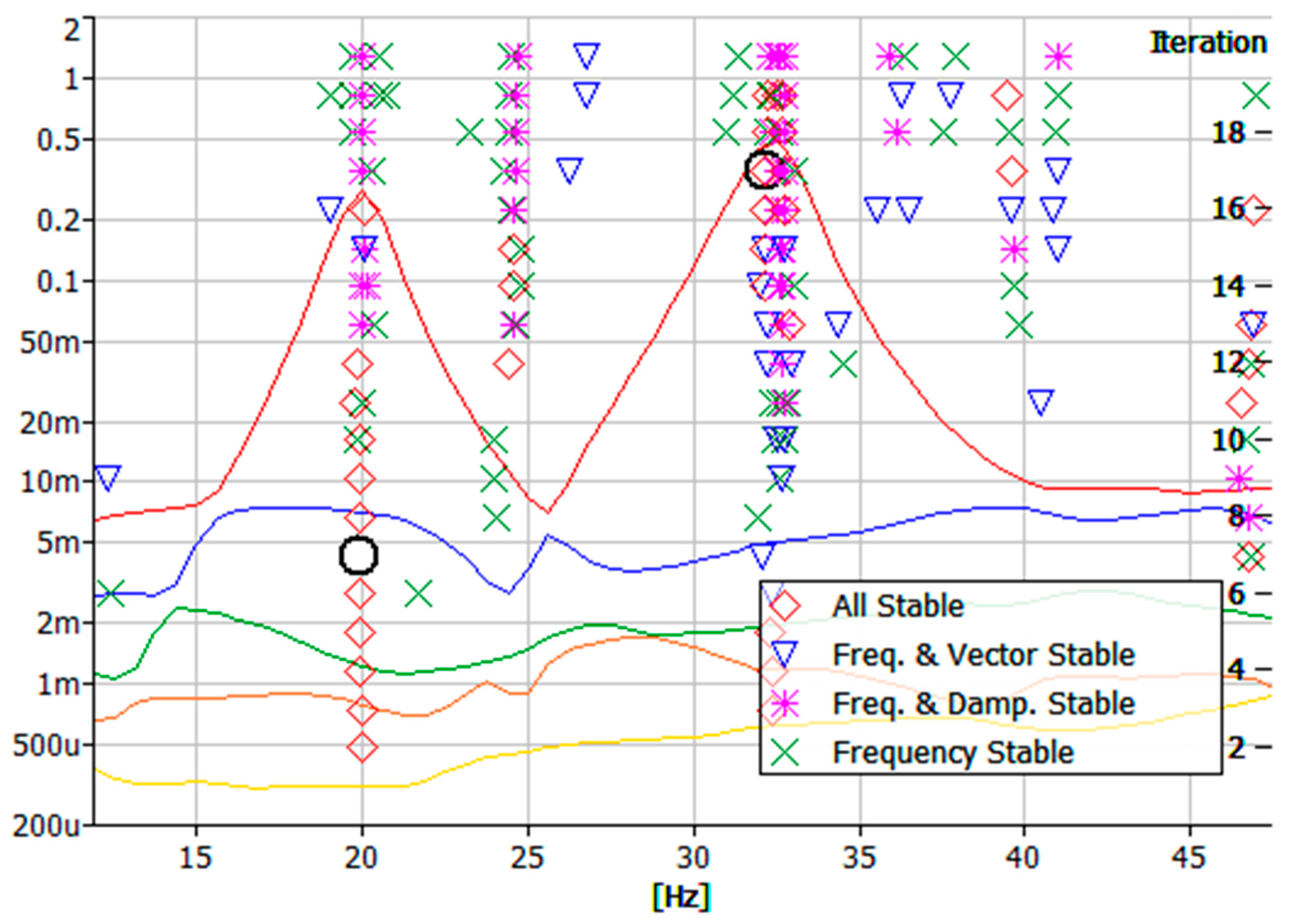
The eigen-frequencies, the mode shapes, and the damping ratios were extracted by applying rational fraction polynomial—Z algorithm in Brüel & Kjær PULSE Connect. The frequency band of FRFs was divided into several parts, which means that identification of poles was restricted in a narrow frequency band each time in order to easily select the stable poles (eigen-frequencies) from the FRFs in each divided frequency range. An example of the stabilization diagram is shown in Figure 4.
Iteration times of rational fraction polynomial—Z algorithm was 40. The synthesized FRF is shown in Figure 5. The corresponding eigen-frequencies and the corresponding damping ratios are shown in Table 1.
Since the measurement system is the SIMO system. Different FRFs (measurement point 11/excitation point 11, measurement point 13/excitation point 13, measurement point 17/excitation point 17, measurement point 24/excitation point 24) can also be saved as references to calibrate the FE model.
3. Finite-Element Model
3.1. Model Description
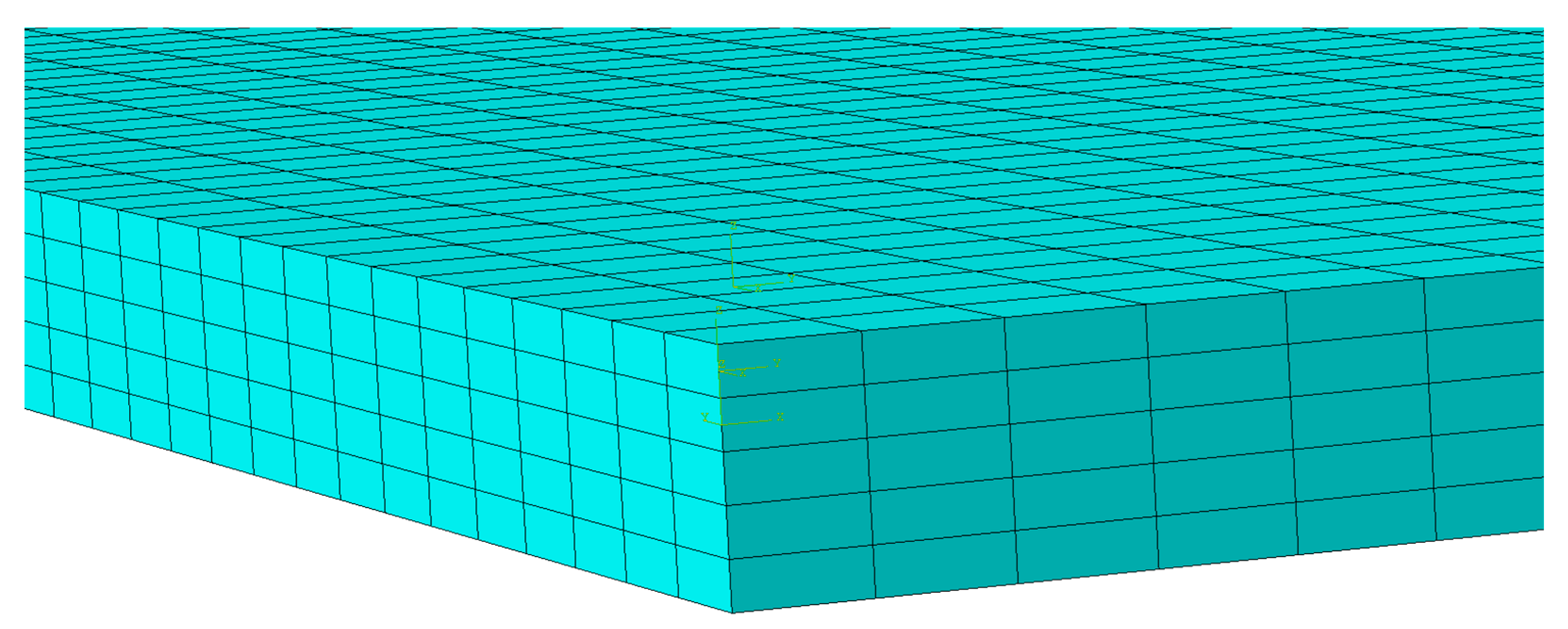
A numerical model of the CLT slab was created in the commercial FE software Abaqus [23]. Five different layers were modelled by assigning different oriented material properties in different layers of the model. Therefore, there is no relative displacement between different layers in this model, which means that the CLT model is a complete model and each layer is fully tied together. The same material was assigned to each layer, except that the in-plan material orientation assignments were 90° oriented from the adjacent layer to mimic the cross-laminate layers of CLT panel. The material properties of CLT were gathered from the literature [24,25], reported in Table 2. The meshes of 20-node quadratic brick, reduced integration (C3D20R) quadratic type were assigned to the entire model. Since the shape of each layer is a simple rectangular so that there is no discontinuity between different layers. Details of mesh are shown in Figure 6. The mesh size was 0.1 to ensure the accuracy of the highest frequency interest. The eigen-frequencies and the eigen-modes were calculated by the linear perturbation frequency step. The FRF of the CLT was obtained by the Steady-state dynamics, Modal step. The damping extracted from the measurement was included in the model by means of the direct modal damping (c.f. Table 1). In this framework, the FRFs of CLT were first calculated to quantify the uncertainties of material properties. Afterward, the best FRF justified by different criterions was selected to extract the material properties of this under investigated CLT.
In general, it is a challenge task to create appropriate constraints to describe the boundary conditions. Since dynamic responses of the structure are sensitive to the boundary conditions, slight changes in the FE model can lead to a big variation of eigen-frequencies and mode order. In order to mimic the simply supported boundary condition, all the displacements in three directions at one shorter edge were constrained and, at the other shorter edge, all the displacements were also constrained except the displacement in a vertical direction (U1 in Abaqus). This boundary set-up of the FE model was kept throughout the entire modelling process. More explanations about the choice of the boundary condition can be found in Section 3.3.
3.2. Model Validation Criterion
The established model needs to be validated by two different metrics. One is the normalized relative frequency difference (NRFD), which characterizes the discrepancies between the simulated and the measured eigen-frequencies, defined by the equation below.
where is the measured resonance frequency and is the simulated resonance frequency.
The other one is the modal assurance criterion (MAC), which quantifies the similarity of simulated and measured mode shapes, defined by the formula below.
where is the i-th simulated mode shape and is the j-th measured mode shape. The range of the MAC number is from 0 to 1. When the MAC number equals 1, the simulated eigen-mode perfectly correlates to the measured one. However, MAC equals 0, which implies irrelevant simulated and measured eigen-modes. Different from the conventional calibration procedure, stochastic process calibration begins with comparing eigen-frequencies (NRFDs) between the simulated FRFs and measured FRFs. Therefore, several FRFs of different positions are needed to make sure the calibrated model validating at different positions, which can increase the credibility of the model. However, the FRFs calibration can only ensure consistency of simulated and measured eigen-frequency but not the mode order. The simulated eigen-frequency may be the same as the measured eigen-frequency, but they could have different mode shapes. Therefore, both indictors are needed to ensure the simulated eigen-frequencies correlated with the measured ones to keep the simulated mode order corresponding to the measured one.
3.3. Preliminary Sensitivity Analysis
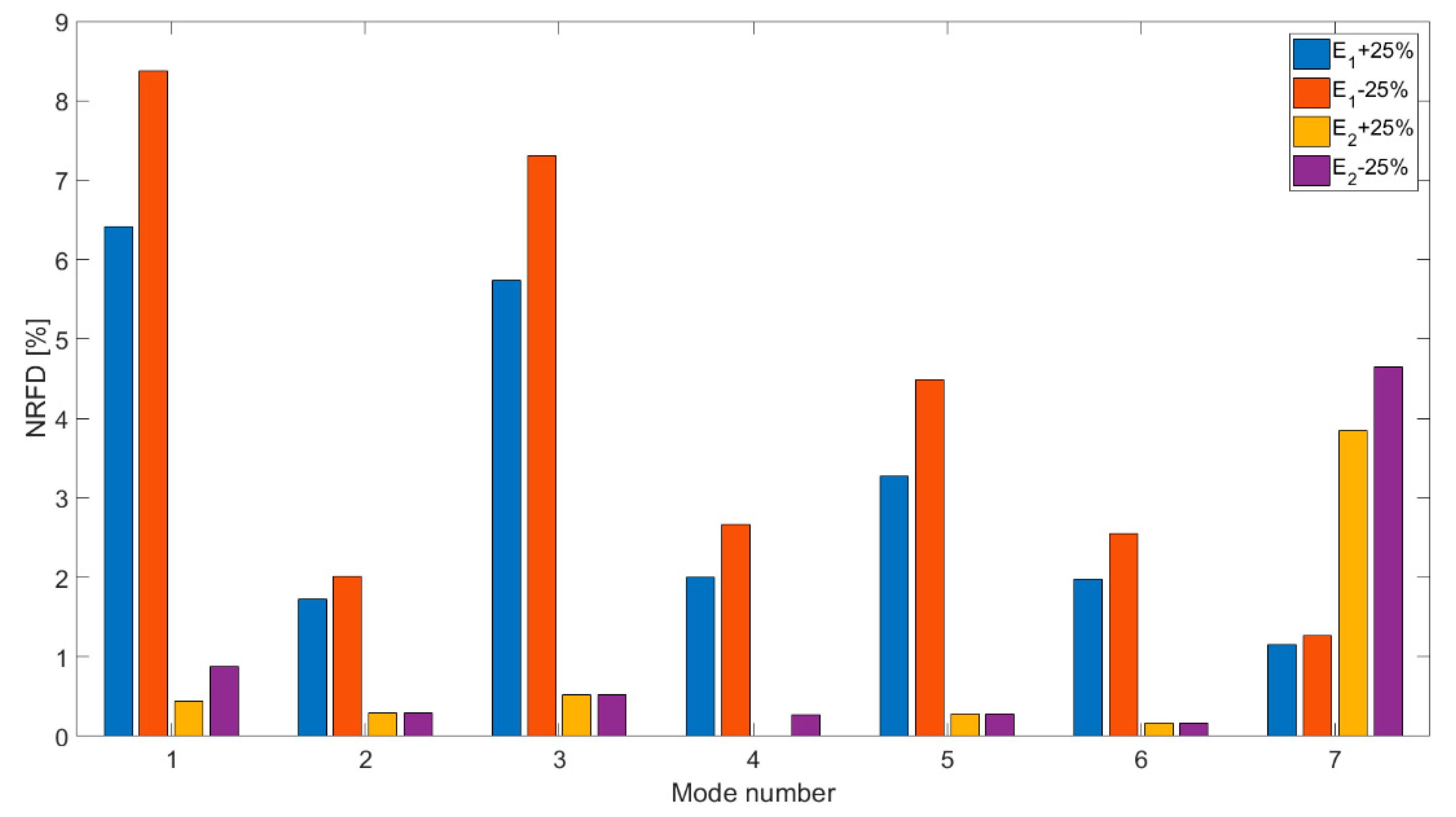
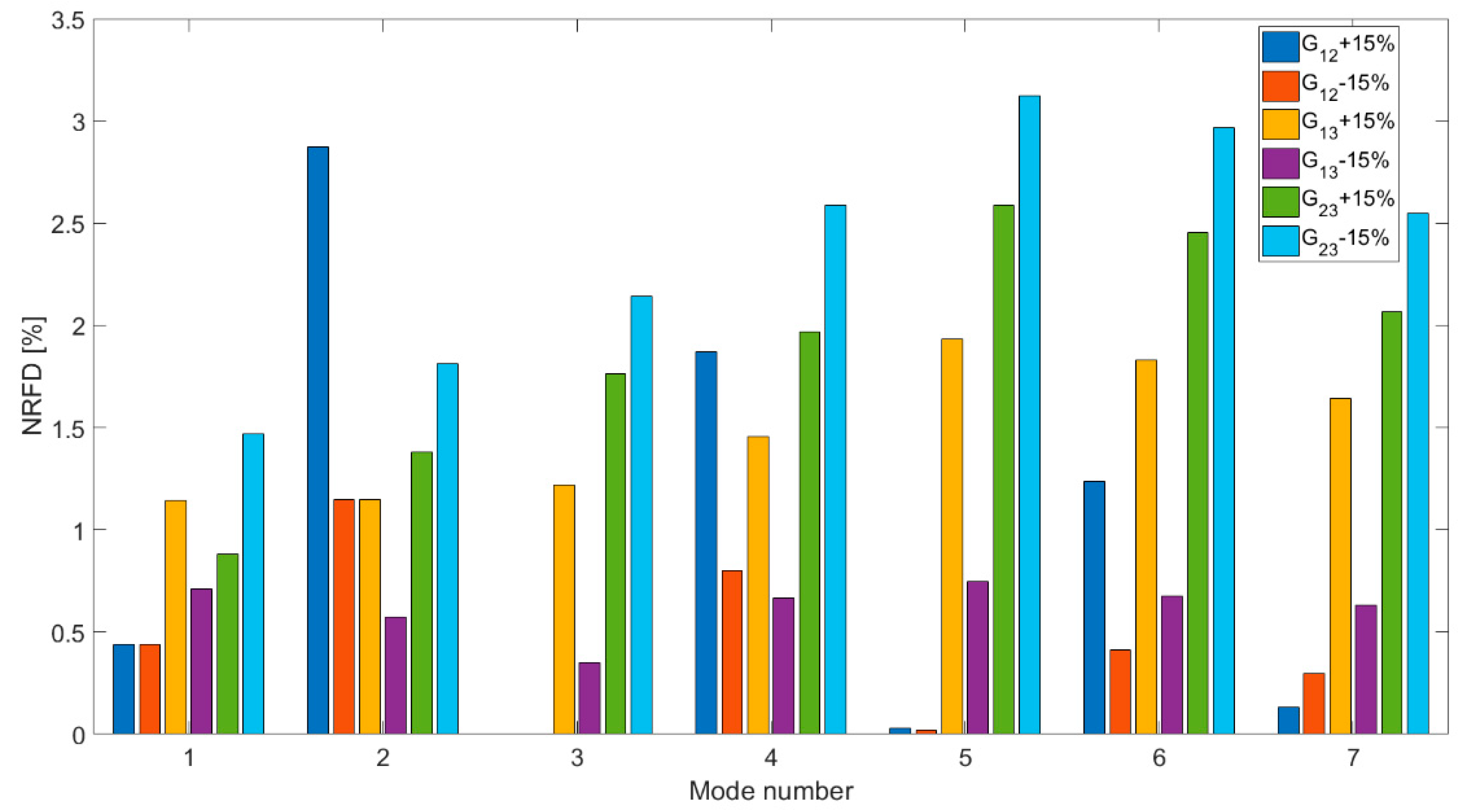
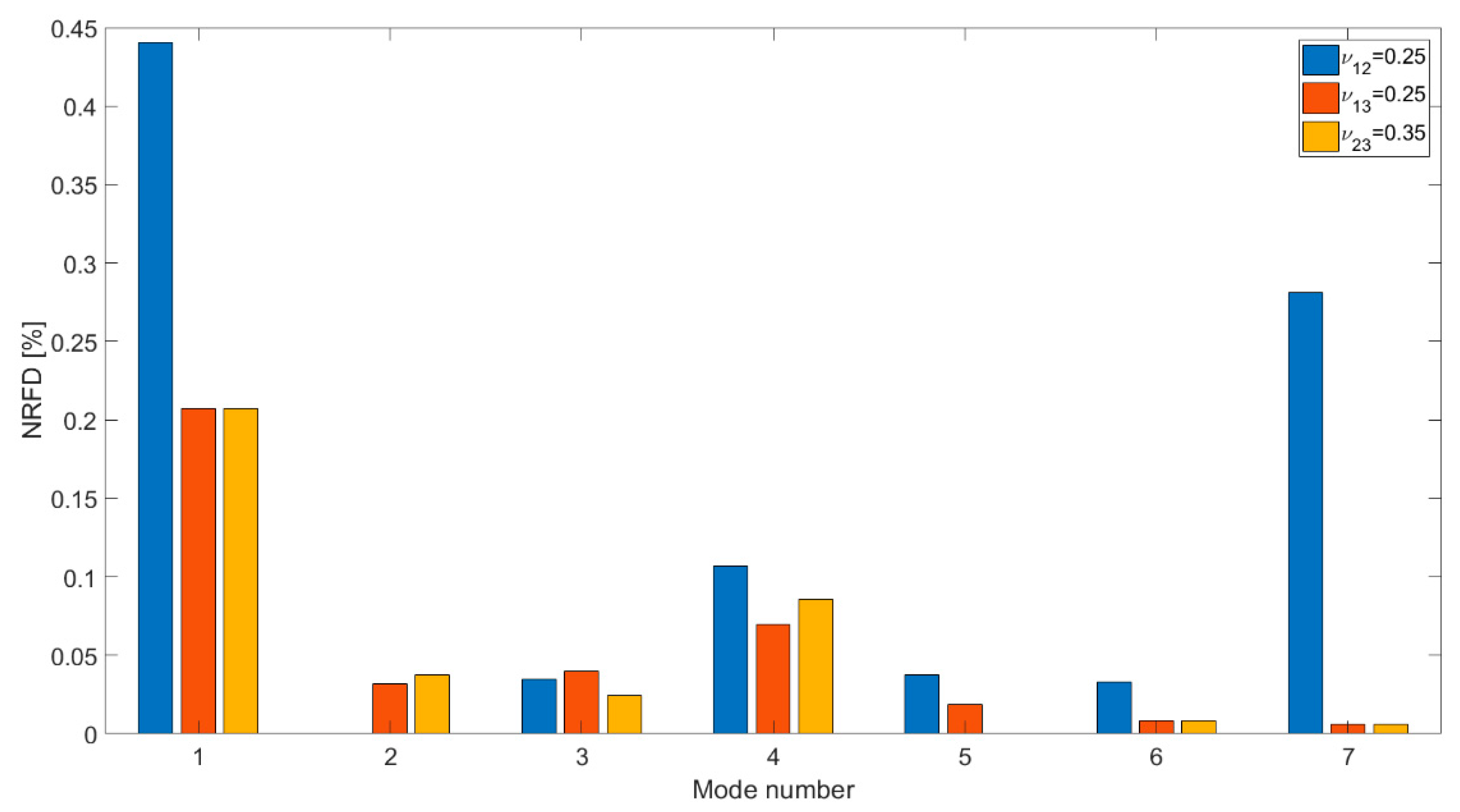
Wood as a kind of orthotropic material has nine different variables (three Young’s moduli, three shear moduli, and three Poisson’s ratios) to be calibrated. In order to decrease the complexity of calibration, a sensitivity analysis should be performed to investigate the effect of different elastic constants on simulated eigen-frequencies before the stochastic process is introduced to the FE model. In this section, Young’s moduli in different directions were increased or decreased 25% when compared to the Young’s moduli given by Table 2. Shear moduli in different directions were increased or decreased 15% when compared to the shear moduli given by Table 2. The Poisson ratios, , , were set to be 0.25, 0.25, and 0.35, whereas the initial values were 0.3, 0.3, and 0.4. The reference eigen-frequencies employed in NRFDs were calculated, according to the elastic constants reported in Table 2. The measured eigen-frequencies were not selected as a reference since the objective of sensitivity analysis aims to investigate how different elastic constants affect the eigen-frequencies of an FE model.
From the NRFDs shown in Figure 7 and Figure 8, it can be seen that the influence of Young’s moduli and shear moduli on eigen-frequencies cannot be ignored. Among all the elastic constants, Young’s modulus in the longitudinal direction has the most important influence on eigen-frequency changes. However, Young’s modulus in a vertical direction barely changes the eigen-frequencies. Therefore, the variation of Young’s modulus in the vertical direction was not reported in Figure 7. When looking at Figure 9, we could find that all the NRFDs are lower than 0.5%, which indicates that the influences of Poisson’s ratios on eigen-frequencies are negligible. From this sensitivity analysis, it can be concluded that the Young’s moduli and shear moduli have a more significant influence on eigen-frequency calculations than Poisson’s ratios. As a result, the calibration of material properties can be reduced to six variables.
However, from this sensitivity analysis, it was also noticed that the first four simulated eigen-frequencies are always higher than the first four measured eigen-frequencies even decreasing different elastic constants. This may be caused by the over-stiffened boundary condition. Since the tested CLT is only placed on the top two steel I beams. It is difficult to have a perfect simply supported boundary conditions in reality. Therefore, restricting all the displacements at the boundaries of the FE model can create over stiffened boundary conditions, which results in over-estimated eigen-frequencies. Consequently, the displacement in a vertical direction at one boundary of the FE model is released to try to mimic the real boundary conditions.
4. Stochastic Process
Uncertainties of material properties are always assumed to follow the Gaussian distribution because of its simplicity and the lack of relevant experimental data, even though most material property distributions are non-Gaussian in nature [26,27]. The theory introduced in this case is about the probabilistic modeling of a random elasticity tensor in an orthotropic symmetric level within the framework of the maximum entropy principle under the constraint of the available information [18,19,28]. The established random elasticity tensor is considered as the inputs in the FE model to quantify the uncertainties induced by the CLT material properties and to seek the best combination of CLT material properties to calibrate the CLT model.
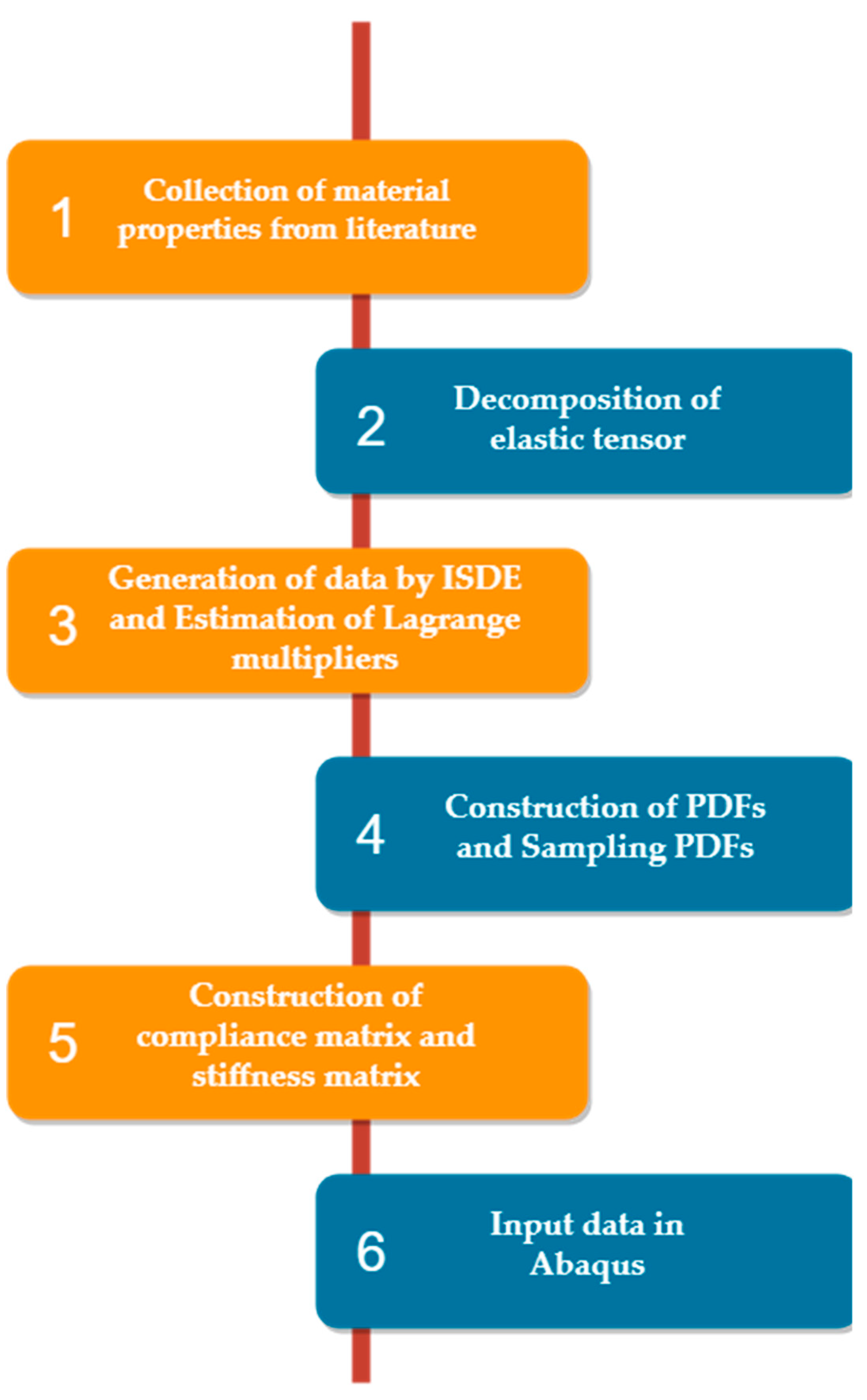
In this section, the elastic tensor is first decomposed in terms of random coefficients and tensor basis so that the fluctuation of different elastic constants can be characterized by the probability distribution functions (PDF). Next, construction of PDFs of different elastic constants in high-dimension [16] is shortly introduced. Lagrange multipliers associated with the explicit PDFs of random variables in high dimensions is estimated with the help of the Itô differential equation. The established PDFs is sampled by Metropolis-Hastings algorithm to obtain the random data to construct a random elasticity matrix [18,19] in order to derive the corresponding random combinations of elasticity constants to quantify the uncertainties of material properties and to calibrate the CLT model. A flow chart of the application of the stochastic procedure is shown in Figure 10.
4.1. Decomposition of the Random Elastic Tensor
Construction of PDF of a random value in a high-dimension approach can be applied to any arbitrary material symmetry class [15,18,19], such as isotropic symmetry, cubic symmetry, and transversely isotropic symmetry. In this work, this stochastic approach aims to seek a reasonable probability distribution of the random elastic tensor of the target material (CLT). Therefore, only the orthotropic symmetry case is considered in this section. The dimension of the random variable is limited to 9.
Let be a fourth-order random elastic tensor, which could be decomposed by using the equation below.
where is a set of random coefficients that can be described by its PDFs and is the tensor basis of the random elastic tensor , based on Walpole’s derivation [29]. The CLT slab is modelled as orthotropic material in Abaqus so that the tensor basis of the orthotropic symmetric elastic tensor are defined in the following form [18].
where , and are the unit orthogonal vectors, is the Kronecker product.
The fourth-order elastic tensor is decomposed as:
4.2. Construction of Probability Distribution Function in High-Dimension Using the Maximum Entropy Principle
The objective of this section is to establish the PDFs of the random coefficients , which control the statistical fluctuation of the fourth-order random elastic tensor. Let be a vector in -valued second order random variable, which obeys certain unknown probability distribution with the Lebesgue measure . The element in vector represent the random coefficient of the random elasticity matrix in the previous section (Equation (3)). The unknown probability distribution of the vector can be presented by a probability density function , which satisfies the following normalization condition.
The Maximum Entropy Principle applied here aims to construct the unknown probability distribution with the help of the available information. In this case, the probability density function (PDF) could be written using the equation below.
where the entropy is defined by the equation below.
In order to find an explicit probability density function , several constraints should be set as available information: (1) the mean values of the variables, (2) the log condition, and (3) the normalization condition.
and
Equation (9) indicates that the mean values of variables are supposed to be known and Equation (10) ensures that both the and are second-order random variables. This equation also creates the statistical dependence between the different random variables.
To optimize the problem defined by Equation (7), Lagrange multipliers associated with Equations (9)–(11) are introduced. Let , and be Lagrange multipliers associated with the constraints defined by Equations (9)–(11). It could be proven that the optimized Equation (7) could be written as [28]:
where is the normalizing constant, the operator is the Euclidean inner product, the is the mapping defined on , with the values in . is defined by Equation (13) below.
where is the support of Equation (13).
An -valued random variable parameterized by should be introduced to identify the Lagrange multipliers. Supposing the probability density function of the random variable is written as:
where is the normalization constant parameterized by . Taking , from Equations (12) and (14), it can be deduced that:
According to Equations (9), (10), (13), and (15), the calculation of Lagrange multipliers can be derived by evaluating the expectation of :
As a result, the problem of the calculation of the Lagrange multipliers converts into generating the independent realizations of the random variable defined over and then evaluating the left-hand side of Equation (16).
4.2.1. Calculation of Lagrange Multipliers
To derive Lagrange multipliers introduced in the previous section, there are several different methods to generate the independent the random variable with respect to the corresponding probability density function (Equation (15)), such as the Metropolis-Hastings method [30,31], Gibbs method [32]. However, it should be noticed that the Metropolis-Hastings method demands an appropriate proposal distribution, which is sometimes difficult to choose, and the Gibbs method requires us to know the conditional distributions. As a consequence, it could be intricate to give a robust calculation without an adequate initial guess, especially for a high-dimension case. Therefore, another alternative algorithm is introduced in Reference [16] to generate the independent random variable .
Random Number Generator
Let be the potential function defined as:
Let be the Markov stochastic process defined on the probability space indexed by with values in , for , satisfying the following Itô stochastic differential equation (ISDE).
where is the normalized Wiener process defined on indexed by and with values in . The probability distribution of the initial condition and are supposed to be known. The parameter is a real positive number, which could dissipate the transition part of the response generated by the initial condition and ensures a reasonable fast convergence of the stationary solution corresponding to the invariant measure.
When tends to infinity, the solution of ISDE converges to the probability distribution of the random variable .
independent realization of is denoted as . Let be the iteration step that the solution of ISDE converge. When the ISDE could be written as the equation below.
Therefore, the independent realizations can be presented by the stationary solution of ISDE.
It is worthwhile to mention that the Itô stochastic differential equation defined by Equation (18) can be discretized by the Explicit Euler scheme to obtain an approximate solution.
with the initial conditions:
where is the iteration step and is a second-order Gaussian centered -valued random variable with a covariance matrix where . In Equation (22), is an -valued random variable, which is the partial derivative of defined by the equation below.
with
Mathematical Expectation Estimation
After the random number generator has been established and the ISDE has been discretized to obtain the random numbers, the expectation of these independent random numbers should be calculated to derive Lagrange multipliers. The mathematical expectation of the random variable can be estimated by using the Monte Carlo method. The evaluation of the mathematical expectation of the random variable is given by the equation below.
After Lagrange multipliers are derived by evaluating the mathematical expectation of the random variable , the explicit PDFs of different elastic elements in the random elasticity matrix can be established. Depending on Equation (12), the PDF of the elastic tensor for the orthotropic symmetric class material could be defined by using the equation below.
with
with
and
Remarks 1.
The random variables,,, andare mutually independent of each other.,, andare Gamma-distributed and theandare the normalization constants.
4.3. Numerical Application of the Orthotropic Symmetric Material (CLT)
The material properties of CLT gathered from the literature (c.f. Table 2) are regarded as an initial starting point (mean value) to procced with the stochastic approach presented in the previous sections.
In Abaqus, the orthotropic materials compliance matrix can be defined by the engineering constants:
The compliance matrix of the CLT panel can be derived depending on the elastic constants reported in Table 2 and Equation (31). The stiffness matrix is the inverse of the compliance matrix.
From Equation (32) and the corresponding orthotropic symmetric matrix basis (Equation (4)), the mean value of defined in Equation (5) can be deduced by using the formulas below.
Let be the target vector to compute the Lagrange multipliers.
And let be the estimated vector to compare with the target vector so that the optimal solution of can be obtained by solving the following optimization function.
where is a free parameter. In this scenario, is set to be 0.5 to give a robust estimation.
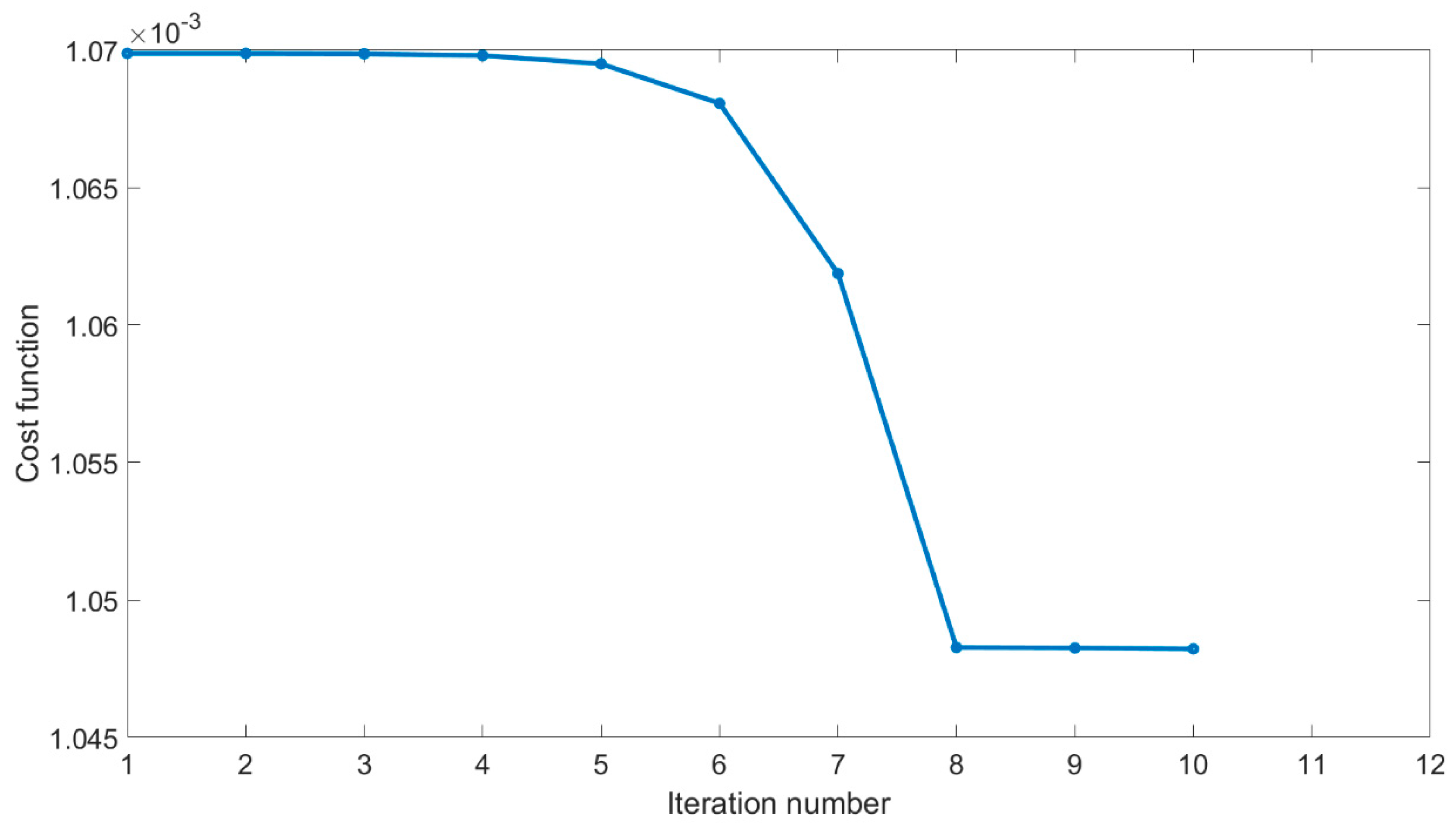
From the sensitivity analysis, the initial guess of is set to be −2. The target optimization function (Equation (35)) is evaluated by using the interior-point method (fmincon function) in Matlab [33].
From Figure 11, it could be observed that the optimization algorithm converges fast to a small value and the corresponding optimal values of the Lagrange multipliers are found to be:
The estimated vector is evaluated by the Monte Carlo method.
Therefore, the estimated vector yields the following.
The cost function of the target vector is , which implies good agreement of the estimated values with the reference values.
4.4. Sampling the Defined Probability Distribution Function by Metropolis-Hastings Alforithm
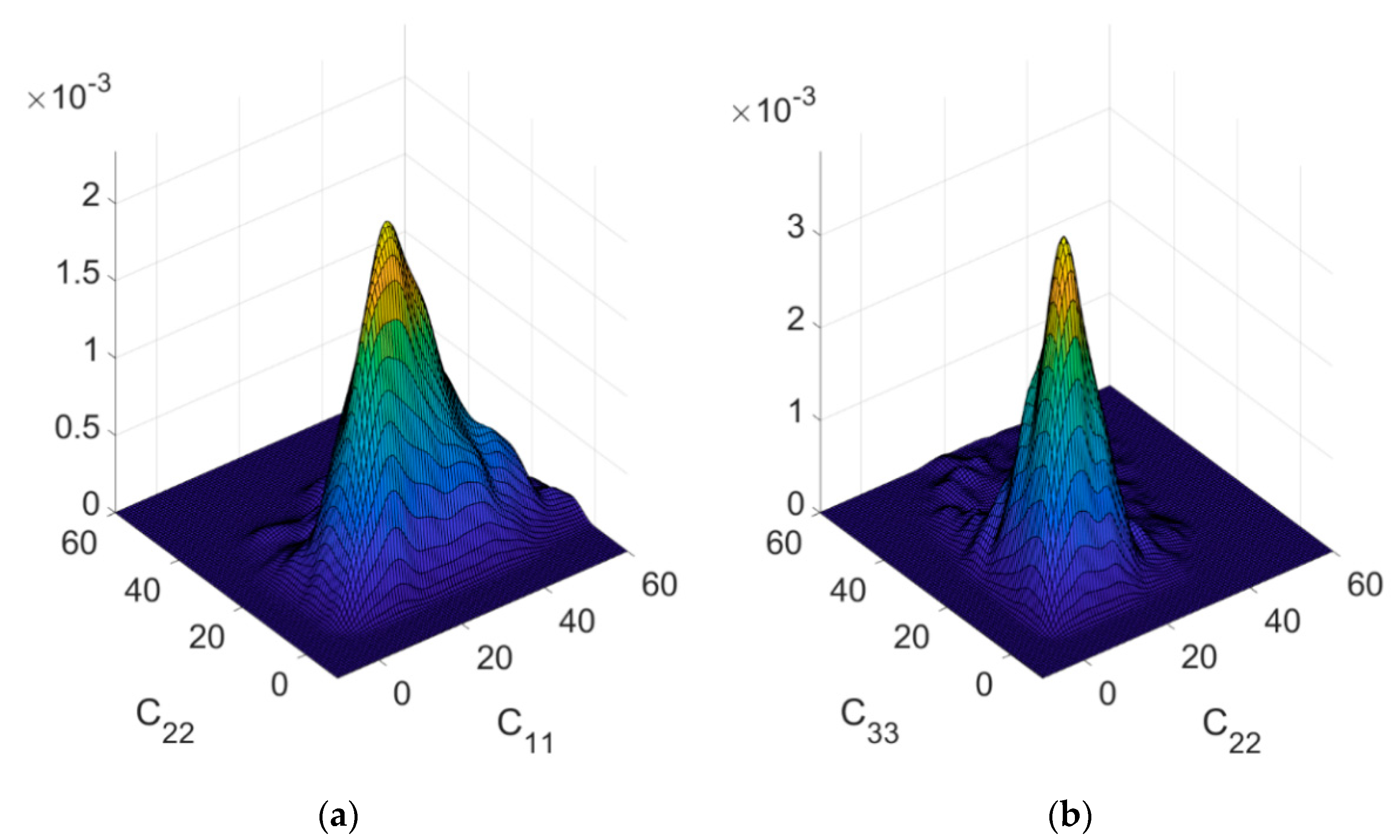
Following the process introduced in the previous section, the PDFs of the random elasticity tensor of the CLT were constructed. The objective of this section is to generate the random numbers that obey the defined PDFs. The corresponding random stiffness matrix of CLT can be constructed following the generated data. Subsequently, the compliance matrix of CLT can be derived by inversing the stiffness matrix. The random elastic constants (engineer constants in Abaqus) of CLT can be determined according to Equation (31). Lastly, the generated elastic constants should be imported into Abaqus to analyze the dynamic response of the CLT panel. The Markov Chain Monte Carlo method is wildly used to sample the high-dimension PDFs. A specific algorithm, called the Metropolis-Hastings algorithm (MHA), is used in this case to sample the target the function. The proposed distribution is a conventional multivariate Gaussian distribution. The mathematical support of is and the mathematical support of is , . When sampling the target function, the generated data should stay in the supports of the sampled function. A total of 50,000 combinations of are realized by performing the MHA and by obeying the mathematical constraints (supports) of the target functions. The marginal distributions of the different mechanical constants reconstructed by ksdensity function in Matlab are shown in Figure 12.
5. Implementation of Stochastic Data in Abaqus
A total of 50,000 generated random numbers have been generated. The corresponding random stiffness tensor could be determined. The random compliance tensor can also be derived by inversing the random stiffness tensor. Since Poisson’s ratios have a very slight influence on the eigen-frequencies and the mode shape order of the CLT numerical model, the variation of the Poisson ratios will not be taken into account in the FE model. 50,000 generated random elastic constants are only satisfied with the mathematical constraints. The constraints associated with the physical meaning are not considered when generating the random numbers. In order to ensure the date implemented in the FE model has physical meanings, several physical constraints are set: (1) Variation of Young’s moduli and shear moduli should be in a reasonable range of wood. The ranges of Young’s modulus and the Shear modulus are assumed in of the respective mean values.
(2) Young’s modulus (Shear modulus) in a principle direction should be larger than the Young’s moduli (Shear moduli) in the other two directions.
(3) Young’s modulus (Shear modulus) in direction 2 should be larger or equal to Young’s modulus (Shear modulus) in direction 3.
Only the generated random elastic constants fulfilled with the above requirements (from Equation (41) to Equation (45)) could be imported in Abaqus. In the work reported in this case, due to limited time and limited computer calculation capacity, only 100 different combinations of elastic constants were selected to calibrate the model and to investigate the influence of material properties on the dynamic response of CLT. This large sum of Abaqus input files with different input mechanical constants were realized with the help of Python scripts.
6. Results and Discussion
6.1. Quantification of Uncertainties
One of the objectives of this article is to investigate the effects of uncertainties induced by material properties on the model output and to ultimately obtain a reliable model to predict the vibro-acoustic behavior of different designs. To achieve that, 100 steady-state simulations with different combinations of material properties were carried out in Abaqus.
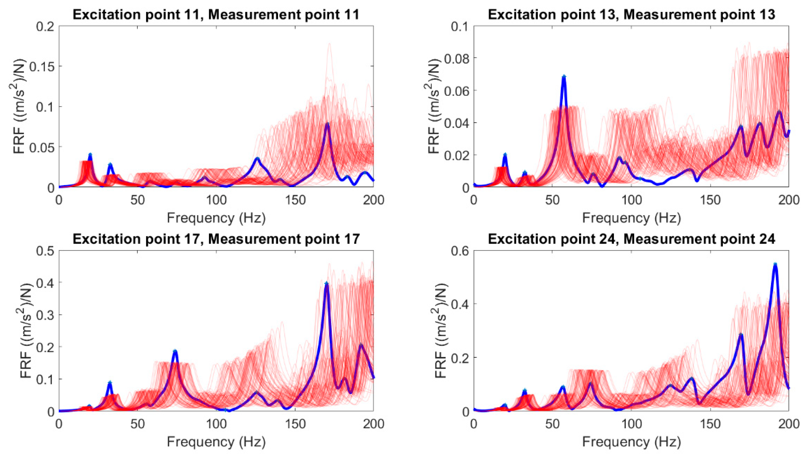
In Figure 13, each subfigure has 100 FRF simulations and the measurement results are shown in blue. Figure 13 shows that there is an obvious envelope overlapped around the first four peaks lower than 100 Hz. The large variation envelope range is due to varying five mechanical constants in one time since five elastic constants variations have a larger impact on the dynamic response of CLT than only changing one elastic constant in one time.
On the contrary of the frequency range lower than 100 Hz, the simulated FRFs begin to scatter above 100 Hz. No clear envelope peaks can be found around the measured resonances higher than 100 Hz. One possible reason of these scattering curves in a relative higher frequency range is the complexity of the mode shapes. It is known that the lower the eigen-frequency is, the simpler the mode shape is and the longer the wave length is. Long wavelength are not sensitive to the small details in the CLT panel, such as the non-uniform air gaps throughout the laminas and the edge bonding (c.f. Figure 14). It implies that the dynamic behavior of CLT in a low frequency range can be mimicked by a simplified homogeneous orthotropic laminated FE model. However, when the mode shapes become more complex in a higher frequency range, the wavelength becomes smaller. As a consequence, small details of the CLT panel begin to affect the vibration of the CLT panel. In this case, the homogeneous orthotropic laminated FE model could not properly describe the dynamic response of the CLT panel in the higher frequency range. In order to increase the accuracy of the FE in a high frequency range, non-homogeneous laminate layer, such as an account for the irregular air gap in laminas, should be modeled. Nevertheless, it should be aware that the calculation time will become longer, when more details are taken into account in the model. The stochastic method needs a large number of calculations to quantify the uncertainties induced by the material properties so that a compromise should be carefully made between the accuracy of the model and the calculation time.
6.2. Calibration of the CLT Panel
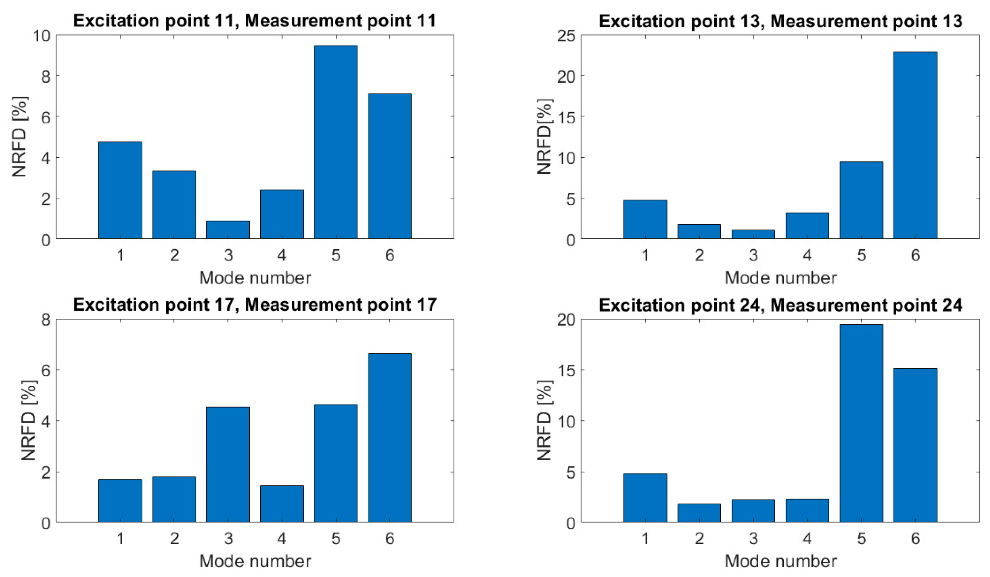
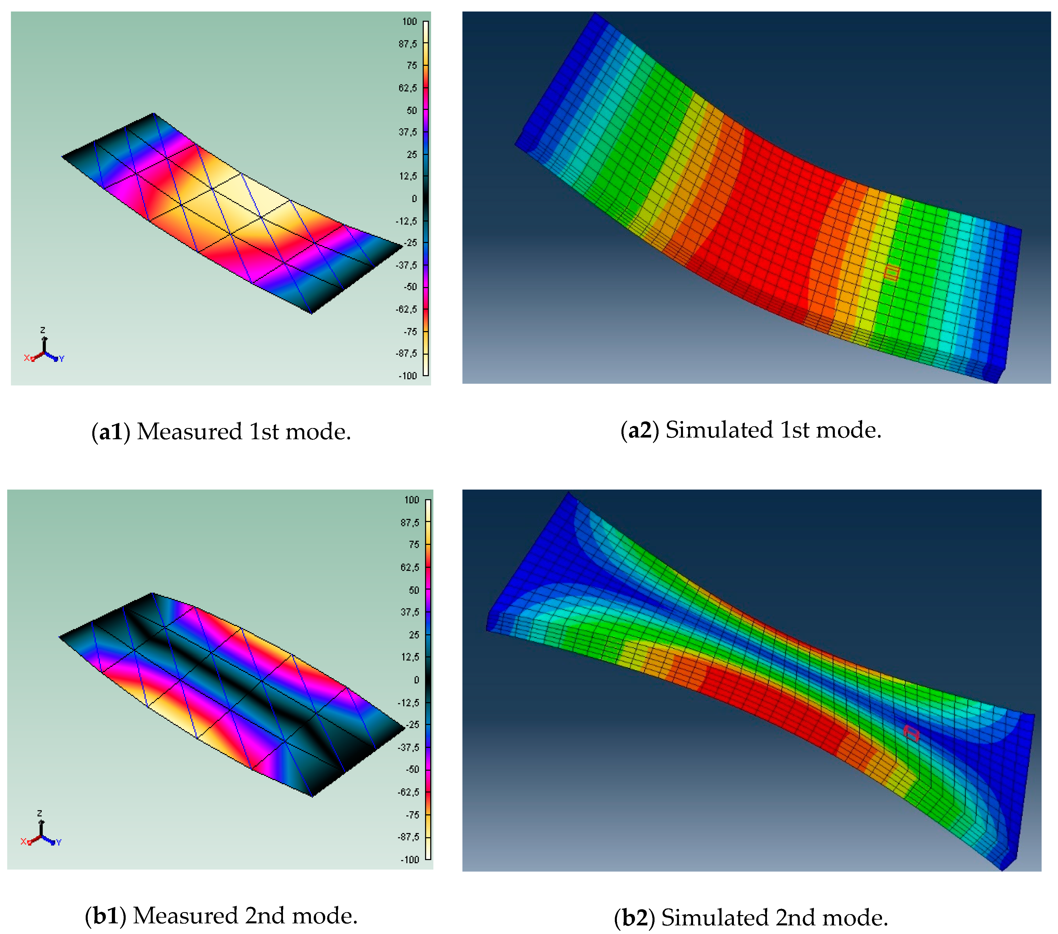
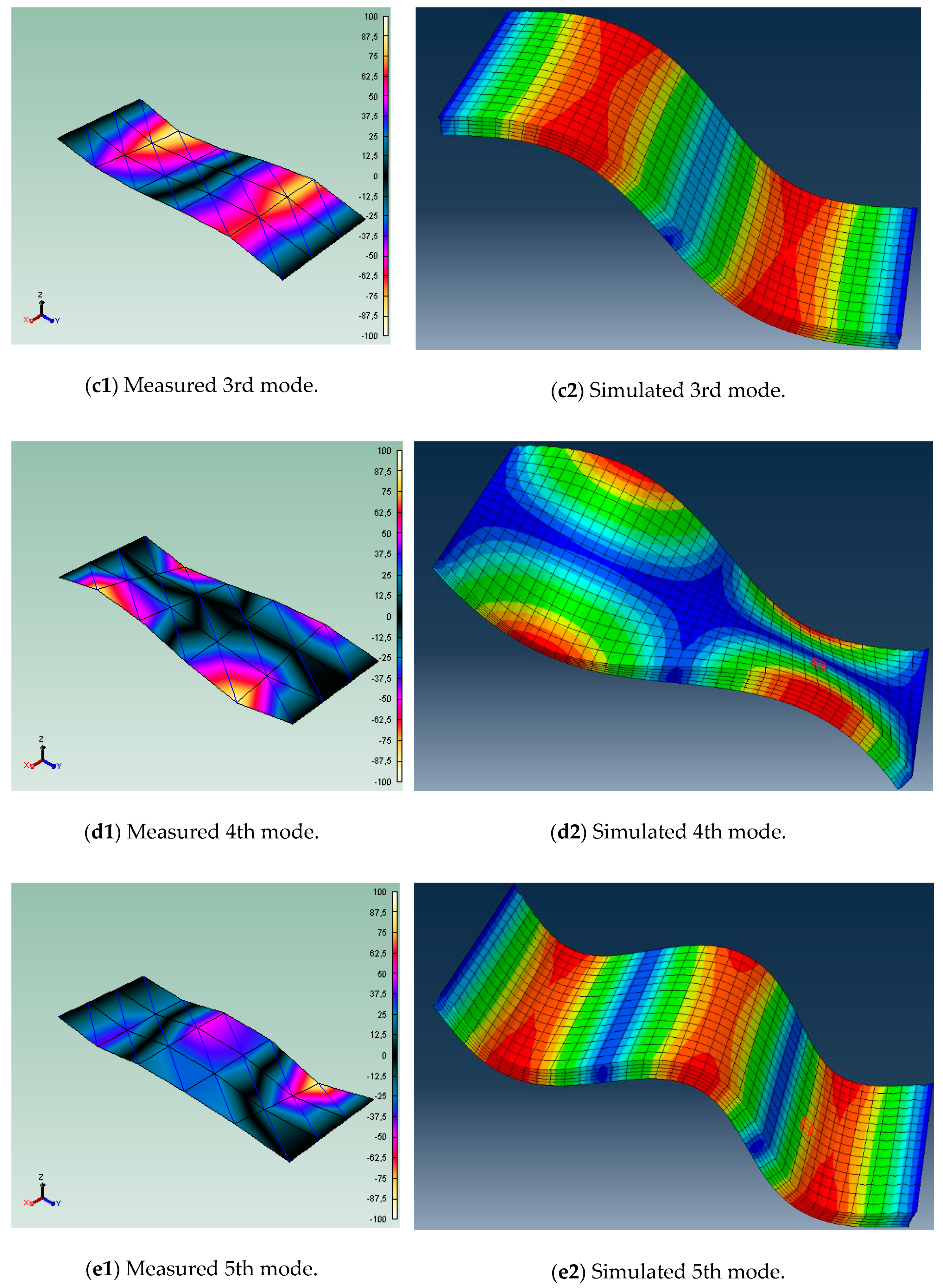
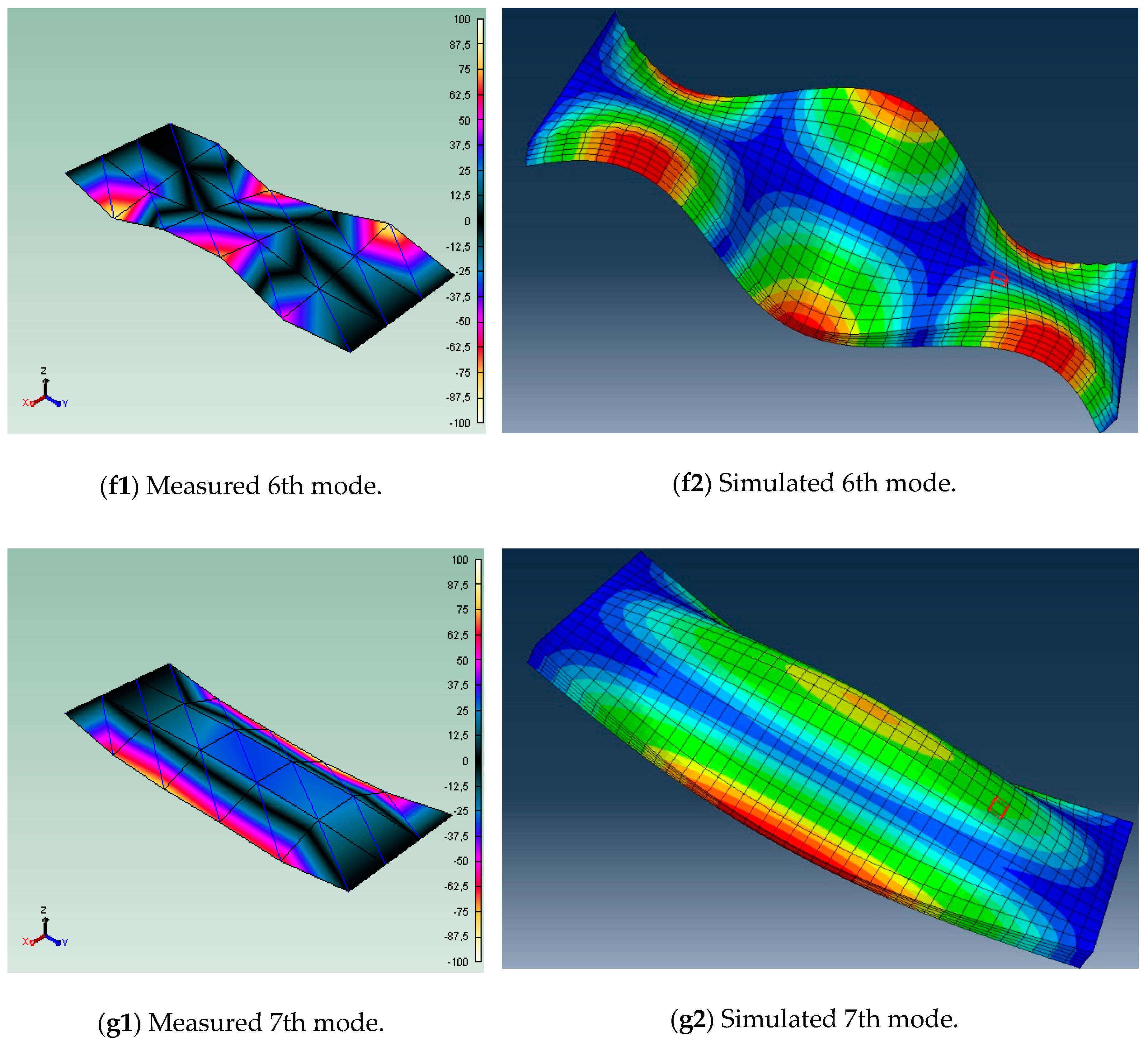
In this section, the best combination of elastic constants of CLT should be identified by selecting the best NRFDs and MACs among 100 simulations. To select the best combination of mechanical constants, the NRFDs of the first four resonances at point 11, point 13, point 17, and point 24 were calculated. The simulations with the smallest NRFDs of the first four resonances at each point were selected from 100 simulations at each point. The NRFDs of the simulated and measured eigen-frequencies at four excitation positions are shown in Figure 15. It can be seen from the NRFDs of each excitation position that the NRFDs of the first four resonances are lower than 5%. However, the NRFDs of the 5th and 6th resonances are relatively high when compared to the first four resonances. This result emphasizes that more structural details should be involved in the FE model to calibrate the dynamic behavior of CLT in the frequency range higher than 100 Hz. However, only NRFD values are not enough to justify the best combination of elastic constants. Since the NRFDs can only represent the simulated eigen-frequency shifts when compared with the experimental results, the mode order can be different even with a low NRFD. Therefore, MAC numbers are needed to validate the model by ensuring the modes in the same order with reference even if there are low NRFDs. The simulated eigen-frequencies and mode shape are reported in Table 1 and Figure 16. The corresponding material properties of CLT are reported in Table 3. Figure 17 shows that the first six simulated modes are in the same order with the measured ones. However, there exist two extra modes in the simulation results.
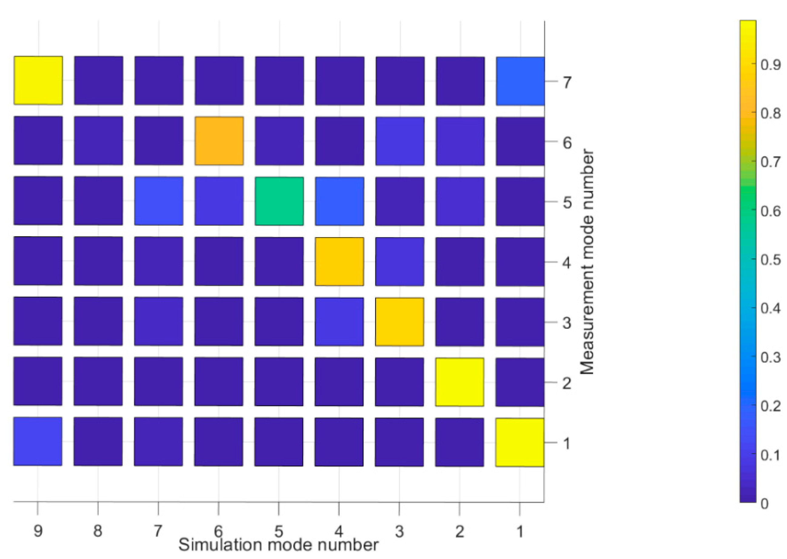
The same results can also be seen in the mobility of different excitation points of the lowest NRFD values (c.f. Figure 18). The simulated FRFs at these four different excitation points correlate better with the measured ones, while there are extra peaks and eigen-frequency shifts in the simulated FRFs in the frequency range from 110 Hz to 170 Hz. We suspect that these discrepancies are higher than the 110 Hz result from the over-simplified homogenous laminated FE model, which ignores the geometrical details contained in the real CLT panel. Yet, the boundary condition set-up in the model could not describe the real measurement boundary conditions.
The dynamic properties of wooden structures highly depend on the material properties of the structure, the geometry details, and the workmanship. Consequently, the deterministic model may not be able to represent the dynamic response of the wooden structures in a realistic way. A calibrated model may not be able to accurately predict the dynamic behavior of the theoretical identical wooden structure due to the uncertainties. The stochastic method is applied in this case to quantify the uncertainties induced by material properties so that this model can estimate the dynamic response of a class of wooden structures, instead of only one structure. Moreover, the influence of material properties on the vibration of CLT is the coupling effect of Young’s moduli and shear moduli in all directions, so that calibration is always time consuming and tedious work to find the appropriate combination of elastic constants in different directions. The calibration employing the stochastic approach could start from the material properties collected from the literature and set the mathematical and physical constraints to generate the input data to find the best combination of the mechanical constants of the under investigated structure. This method could automate the calibration step to avoid the repetitive manual calibrations. However, we should pay attention to the mathematical and physical constraints before generating the input elastic constant data. Because the generated elastic constants should be in a reasonable range of the under investigated material. Otherwise, the input elastic constants may not have a physical meaning, even though the calibration results fit well with the reference. The stochastic method uses a large amount of data to describe an unknown problem (the data base of CLT in our case). More calculations are made and more accurate calibration can be achieved. However, a trade-off between the calculation time and the accuracy of the result should be made in order to keep the calculation time in a reasonable range. This method can not only be applied to CLT but also can be employed to calibrate the other wooden structures whose stiffness constants are difficult to obtain.
Furthermore, one of the objectives of this stochastic approach is to calibrate the material properties of the target structure. It would be better to decrease the influence of other influence factors, such as boundary conditions. Therefore, it is suggested to hang up the under investigated structure (free-free boundary condition) or fix the structure boundary to the ground (perfect simply supported condition) to eliminate the influence of boundary conditions as far as possible. In the work reported in this case, due to a lack of support materials, the CLT panel just laid on top of the I-steel beam and it was not screwed into the ground. Consequently, when the CLT is excited, the deformation of the I-steel beam can affect the vibration of the CLT slab. Furthermore, the laboratory boundary conditions are always different from the in-situ boundary conditions [34]. Thus, it would be necessary to investigate the dynamic response of CLT in a real building. To achieve that, the FRFs could be first measured from a CLT bare floor in real mounting conditions. Then, the same CLT bare floor could be set in the simplified laboratory conditions to compare the relative differences between different FRFs under different boundary conditions.
From the FE CLT modelling perspective, the model validation criterions (NRFD and MAC) and the simulated FRFs suggest that dynamic behavior of the CLT panel can be modelled by the homogenous orthotropic laminated FE model in the frequency range lower than 100 Hz. In a higher frequency range, as the inhomogeneity of the laminated layers of CLT slab begins to pronounce in the vibration of CLT panel, more geometrical details in the CLT panel should be taken into account in the FE CLT model to obtain more accurate results.
7. Conclusions
Low frequency sound insulation is always a challenge for the wooden constructions, especially for the multi-family dwellings. Even though the wooden constructions are satisfied with the standards in force, acoustic comfort is not always met. Since the evaluation frequency range even with the adaptation term of the current standards is from 50 Hz to 3150 Hz, however, the first few resonance frequencies of the wooden floor, which are believed to cause most annoyances, are left out of the evaluation scope. Low frequency prediction tools are needed to access the vibratory performance of wooden buildings at the early design stage due to complaints coming from the inhabitants in wooden buildings. Accessing an accurate low frequency prediction tool requires involving the structure details in the model. Moreover, material properties are another important factor, which can induce a remarkable change in the modelling output.
In this paper, we introduced the stochastic process into the FE model to quantify the uncertainties generated by the material properties. By performing Monte Carlo simulations, variation of Young’s moduli and shear moduli in different directions were taken into account in FE model to investigate the coupling effect of different elastic moduli on the dynamic response of structure. Furthermore, 100 simulations were calculated at four different driving points. Clear envelopes can be observed from the simulations lower than 100 Hz. However, the simulations begin to scatter in the frequency range higher than 100 Hz. The best combination of material properties is selected from 100 different combinations of elastic constants to calibrate the FE CLT model. It was noticed that the simulated dynamic response that was lower than 100 Hz was correlated better with the measured dynamic response of CLT. From the promising results, it was concluded that the stochastic method can be applied to a deterministic model (FE model) to quantify the uncertainties of the structures. Furthermore, this method can be employed to calibrate the FE model to acquire the material properties of the under-investigated structure.
Author Contributions
Data curation, C.Q. Investigation, C.Q. Methodology, C.Q. and J.N. Supervision, S.M. and D.B. Validation, C.Q. Visualization, C.Q. Writing—original draft, C.Q. Writing—review & editing, C.Q. and J.N.
Funding
The authors are grateful to FPInnovation and Nordic Structure and Industrial Chair on Eco-responsible Wood Construction (CIRCERB).
Conflicts of Interest
The authors declare no conflict of interest.
References
- Späh, M.; Hagberg, K.; Barlome, O.; Weber, L.; Leistner, P.; Liebl, A. Subjective and Objective Evaluation of Impact Noise Sources in Wooden Buildings. Build. Acoust. 2013, 20, 193–213. [Google Scholar] [CrossRef]
- Sipari, P. Sound Insulation of Multi-Storey Houses—A Summary of Finnish Impact Sound Insulation Results. Build. Acoust. 2000, 7, 15–30. [Google Scholar] [CrossRef]
- Ljunggren, F.; Simmons, C.; Hagberg, K. Correlation between sound insulation and occupants’ perception –Proposal of alternative single number rating of impact sound. Appl. Acoust. 2014, 85, 57–68. [Google Scholar] [CrossRef]
- Vardaxis, N.G.; Bard, D.; Persson, W. Review of acoustic comfort evaluation in dwellings—part I: Associations of acoustic field data to subjective responses from building surveys. Build. Acoust. 2018, 25, 151–170. [Google Scholar] [CrossRef]
- Forssén, J.; Kropp, W.; Brunskog, S.; Ljunggren, S.; Bard, D.; Sandberg, G.; Ljunggren, F.; Agren, A.; Hallstrom, O.; Dybro, H.; et al. Acoustics in Wooden Buildings: State of the Art 2008; Vinnova Project 2007-01653; SP Technical Research Institute of Sweden: Stockholm, Sweden, 2008. [Google Scholar]
- Flodén, O.; Persson, K.; Sandberg, G. Numerical methods for predicting vibrations in multi-story wood buildings. In Proceedings of the World Conference On Timber Engineering, Vienna, Austria, 22–25 August 2016. [Google Scholar]
- ISO717-2. Acoustics—Rating of sound insulation in buildings and of building elements. In Part 2: Impact Sound Insulation; International Organization for Standardization: Geneva, Switzerland, 2013. [Google Scholar]
- Bolmsvik, A.; Linderholt, A.; Jarnerö, K. FE modeling of a lightweight structure with different junctions. In Proceedings of the European Conference on Noise Control, Prague, Czech Republic, 10–13 June 2012; pp. 162–167. [Google Scholar]
- Wang, P.; Van Hoorickx, C.; Dijckmans, A.; Lombaert, G.; Reynders, E. Numerical prediction of impact sound in dwelling from low to high frequencies. In Proceedings of the INTER-NOISE 2018—47th International Congress and Exposition on Noise Control Engineering: Impact of Noise Control Engineering, Chicago, IL, USA, 26–29 August 2018. [Google Scholar]
- Negreira, J.; Sjöström, A.; Bard, D. Low frequency vibroacoustic investigation of wooden T-junctions. Appl. Acoust. 2016, 105, 1–12. [Google Scholar] [CrossRef]
- Flodén, O.; Persson, K.; Sandberg, G. A multi-level model correlation approach for low-frequency vibration transmission in wood structures. Eng. Struct. 2018, 157, 27–41. [Google Scholar] [CrossRef]
- Coguenanff, C. Robust Design of Lightweight Wood-Based Systems in Linear Vibroacoustics. Doctoral Thesis, Université Paris-Est, Paris, France, October 2015. [Google Scholar]
- Persson, P.; Flodén, O. Towards Uncertainty Quantification of Vibrations in Wood Floors. In Proceedings of the 25th International Congress on Sound and Vibration, Hiroshima, Japan, 8–12 Junly 2018. [Google Scholar]
- Shannon, C.E. A Mathematical Theory of Communication. Bell Syst. Tech. J. 1948, 27, 379–423. [Google Scholar] [CrossRef]
- Staber, B.; Guilleminot, J. Approximate Solutions of Lagrange Multipliers for Information-Theoretic Random Field Models. SIAM/ASA J. Uncertain. Quantif. 2015, 3, 599–621. [Google Scholar] [CrossRef]
- Soize, C. Construction of probability distributions in high dimension using the maximum entropy principle: Applications to stochastic processes, random fields and random matrices. Int. J. Numer. Method. Eng. 2008, 76, 1583–1611. [Google Scholar] [CrossRef]
- Soize, C. Stochastic Models of Uncertainties in Computational Mechanics; American Society of Civil Engineer: Reston, VA, USA, 2012; ISBN 978-0-7844-1223-7. [Google Scholar]
- Guilleminot, J.; Soize, C. On the Statistical Dependence for the Components of Random Elasticity Tensors Exhibiting Material Symmetry Properties. J. Elast. 2013, 111, 109–130. [Google Scholar] [CrossRef]
- Guilleminot, J.; Soize, C. Generalized stochastic approach for constitutive equation in linear elasticity: A random matrix model. Int. J. Numer. Method. Eng. 2012, 90, 613–635. [Google Scholar] [CrossRef]
- Martini, A.; Troncossi, M.; Vincenzi, N. Structural and Elastodynamic Analysis of Rotary Transfer Machines by Finite Element Model. J. Serb. Soc. Comput. Mech. 2017, 11. [Google Scholar] [CrossRef]
- Manzato, S.; Peeters, B.; Osgood, R.; Luczak, M. Wind turbine model validation by full-scale vibration test. In Proceedings of the European Wind Energy Conference (EWEC) 2010, Warsaw, Poland, 20–23 April 2010. [Google Scholar]
- Brüel & Kjær. Product data—Heavy Duty Impact Hammers—Type 8207, 8208 and 8210; Brüel & Kjær Sound and Vibration Measurement A/S: Nærum, Denmark, 2012. [Google Scholar]
- ABAQUS/CAE, 2017. Dassault Systèmes SIMULIA: Vélizy-Villacoublay, France, 2017.
- Zhou, J.H.; Chui, Y.H.; Gong, M.; Hu, L. Elastic properties of full-size mass timber panels: Characterization using modal testing and comparison with model predictions. Compos. Part Eng. 2017, 112, 203–212. [Google Scholar] [CrossRef]
- Ussher, E.; Arjomandi, K.; Weckendorf, J.; Smith, I. Prediction of motion responses of cross-laminated-timber slabs. Structures 2017, 11, 49–61. [Google Scholar] [CrossRef]
- Shang, S.; Yun, G.J. Stochastic finite element with material uncertainties: Implementation in a general purpose simulation program. Finite Elem. Anal. Des. 2013, 64, 65–78. [Google Scholar] [CrossRef]
- Stefanou, G. The stochastic finite element method: Past, present and future. Comput. Methods Appl. Mech. Eng. 2009, 198, 1031–1051. [Google Scholar] [CrossRef]
- Soize, C. Random matrix theory for modeling uncertainties in computational mechanics. Comput. Methods Appl. Mech. Eng. 2005, 194, 1333–1366. [Google Scholar] [CrossRef]
- Walpole, L.J. Fourth-rank tensors of the thirty-two crystal classes: Multiplication tables. Proc. R. Soc. Lond. Math. Phys. Sci. 1984, 391, 149–179. [Google Scholar] [CrossRef]
- Chib, S.; Greenberg, E. Understanding the Metropolis-Hastings Algorithm. Am. Stat. 1995, 49, 327–335. [Google Scholar]
- Robert, P.C.; Casella, G. Monte Carlo Statistical Methods; Springer: New Yourk, NY, USA, 2013. [Google Scholar]
- Kroese, P.D.; Taimre, T.; Botev, Z. Handbook of Monte Carlo Methods; John Wiley & Sons: Hoboken, NJ, USA, 2010. [Google Scholar]
- Matlab, R2017b. The MathWorks Inc.: Natick, MA, USA, 2017.
- Martini, A.; Troncossi, M. Upgrade of an automated line for plastic cap manufacture based on experimental vibration analysis. Case Stud. Mech. Syst. Signal Process. 2016, 3, 28–33. [Google Scholar] [CrossRef]
Figure 1.
(a) Two CLT panels connected by a thin wooden lath. (b) One CLT panel simply supported on two I-steel beams.
Figure 1.
(a) Two CLT panels connected by a thin wooden lath. (b) One CLT panel simply supported on two I-steel beams.

Figure 2.
Mesh on the CLT panel. Five accelerometers (red dots) were placed at points 10, 11, 13, 17, and 24), whereas the hammer was moved around all nodes, except on the short edges.
Figure 2.
Mesh on the CLT panel. Five accelerometers (red dots) were placed at points 10, 11, 13, 17, and 24), whereas the hammer was moved around all nodes, except on the short edges.

Figure 3.
(a) Impulse shapes of the hammers showing the shape as a function of the used impact tip. (b) Force spectra of the hammers showing the frequency response as a function of used impact tip [22] Copyright © Brüel & Kjær.
Figure 3.
(a) Impulse shapes of the hammers showing the shape as a function of the used impact tip. (b) Force spectra of the hammers showing the frequency response as a function of used impact tip [22] Copyright © Brüel & Kjær.

Figure 4.
Stabilization diagram with rational fraction polynomial—Z algorithm.

Figure 5.
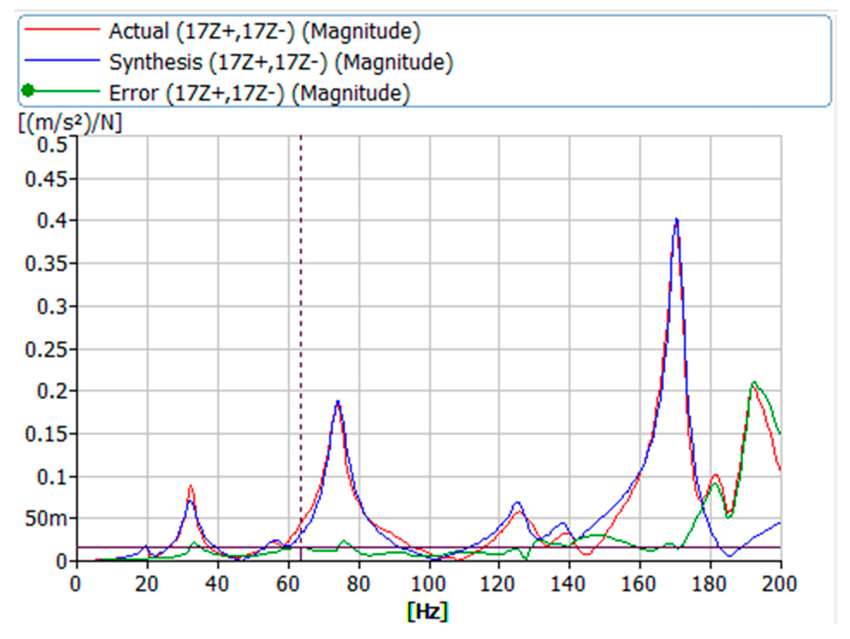
Synthesized FRF, measured FRF, and relative errors between the synthesized FRF and the measured FRF.
Figure 5.
Synthesized FRF, measured FRF, and relative errors between the synthesized FRF and the measured FRF.

Figure 6.
Meshes of FE CLT model.

Figure 7.
NRFDs of Young’s moduli.

Figure 8.
NRFDs of shear moduli.

Figure 9.
NRFDs of Poisson’s ratios.

Figure 10.
Flow chart of the application of the stochastic process.

Figure 11.
Convergence of the optimization algorithm.

Figure 12.
(a) Joint probability density function of random variables and . (b) Joint probability density function of random variables and .
Figure 12.
(a) Joint probability density function of random variables and . (b) Joint probability density function of random variables and .

Figure 13.
Measured (blue) and simulated (red) FRFs at point 11, 13, 17, and 24.

Figure 14.
(a) Air gaps in the laminate layers of CLT. (b) No edge-bonding of CLT.

Figure 15.
NRFDs of the first six resonances at points 11, 13, 17, and 24.

Figure 16.
Measured and simulated modes.


Figure 17.
Cross-MAC.

Figure 18.
Magnitude of the complex mobility in the vertical direction of point 11, 13, 17, and 24. Simulated FRFs in red, measured FRFs in blue.
Figure 18.
Magnitude of the complex mobility in the vertical direction of point 11, 13, 17, and 24. Simulated FRFs in red, measured FRFs in blue.


Table 1.
Measured and simulated Eigen frequencies of the bending modes and the measured corresponding damping ratios.
Table 1.
Measured and simulated Eigen frequencies of the bending modes and the measured corresponding damping ratios.
| Mode | Measured Eigen-Frequency/Simulated Eigen-Frequency | Damping Ratio |
|---|---|---|
| 1 | 19.8 Hz/19 Hz | 4.9% |
| 2 | 32.2 Hz/33.2 Hz | 3.6% |
| 3 | 56.7 Hz/58.3 Hz | 3.2% |
| 4 | 73.8 Hz/72.5 Hz | 3.2% |
| 5 | 91.0 Hz/100.8 Hz | 3.3% |
| 6 | 125.5 Hz/117 Hz | 2.8% |
| - | -/131 Hz | - |
| - | -/150 Hz | - |
| 7 | 170.4 Hz/173.9 Hz | 1.2% |
Table 2.
Material Properties of CLT collected from the literature. Stiffness parameters have the unit of MPa, Poisson ratios are dimensionless, and the density is given in kg/m3.
Table 2.
Material Properties of CLT collected from the literature. Stiffness parameters have the unit of MPa, Poisson ratios are dimensionless, and the density is given in kg/m3.
| E1 | E2 | E3 | G12 | G13 | G23 | ||||
|---|---|---|---|---|---|---|---|---|---|
| 9200 | 4000 | 4000 | 900 | 90 | 63 | 0.3 | 0.3 | 0.4 | 520 |
Table 3.
Material Properties of CLT used in the calibrated FE model. Stiffness parameters have the unit of MPa and the density is given in kg/m3.
Table 3.
Material Properties of CLT used in the calibrated FE model. Stiffness parameters have the unit of MPa and the density is given in kg/m3.
| E1 | E2 | E3 | G12 | G13 | G23 | ||||
|---|---|---|---|---|---|---|---|---|---|
| 13,396 | 4712.5 | 4681.6 | 974.6 | 63.64 | 60.46 | 0.4 | 0.4 | 0.3 | 520 |
© 2019 by the authors. Licensee MDPI, Basel, Switzerland. This article is an open access article distributed under the terms and conditions of the Creative Commons Attribution (CC BY) license (http://creativecommons.org/licenses/by/4.0/).
Share and Cite
MDPI and ACS Style
Qian, C.; Ménard, S.; Bard, D.; Negreira, J. Development of a Vibroacoustic Stochastic Finite Element Prediction Tool for a CLT Floor. Appl. Sci. 2019, 9, 1106. https://doi.org/10.3390/app9061106
AMA Style
Qian C, Ménard S, Bard D, Negreira J. Development of a Vibroacoustic Stochastic Finite Element Prediction Tool for a CLT Floor. Applied Sciences. 2019; 9(6):1106. https://doi.org/10.3390/app9061106
Chicago/Turabian StyleQian, Cheng, Sylvain Ménard, Delphine Bard, and Juan Negreira. 2019. "Development of a Vibroacoustic Stochastic Finite Element Prediction Tool for a CLT Floor" Applied Sciences 9, no. 6: 1106. https://doi.org/10.3390/app9061106
Note that from the first issue of 2016, this journal uses article numbers instead of page numbers. See further details here.