Simulation of Truck Haulage Operations in an Underground Mine Using Big Data from an ICT-Based Mine Safety Management System


Department of Energy Resources Engineering, Pukyong National University, Busan 48513, Korea
*
Author to whom correspondence should be addressed.
Appl. Sci. 2019, 9(13), 2639; https://doi.org/10.3390/app9132639
Submission received: 21 April 2019
/
Revised: 25 June 2019
/
Accepted: 27 June 2019
/
Published: 29 June 2019
(This article belongs to the Special Issue Emerging Technologies for Harnessing the Fourth Industrial Revolution in the Energy and Mineral Industries)
Abstract
:Information communication technology (ICT)-based mine safety management systems are being introduced at numerous mining sites to track the location of equipment and workers in real time and monitor environmental changes. This paper presents the results of a case study in which the big data created by an ICT-based mine safety management system are used for simulating truck haulage operations. An underground limestone mine located in Danyang, South Korea was studied, and the data generated over three months, from October 1 to December 31, 2018, were analyzed. Truck tag packet data recognized by relays were extracted and analyzed to calculate the averages and standard deviations of the truck travel times of each mine segment. A discrete event simulation program that simulates truck haulage operations in the study area was developed. Haulage times, the number of haulage operations, production output, and truck delay times were predicted, and results were compared with the actual operation results that were obtained on January 2 and 9, 2019. The difference between the predicted and actual results for the total amount of loaded ore was 30 tons for January 2 and 0 tons for January 9. The mean absolute error between the predicted and observed truck travel times was 0.13 min for January 2 and 0.14 min for January 9. The truck travel times that were measured differently according to the data aggregation period were set as temporal factors, and truck haulage simulations were performed. The results showed that more reliable simulation results were obtained as data accumulation time increased.
1. Introduction
1.1. Mine Safety Management System for Underground Mines
Fatal worker accidents frequently occur in underground mines owing to their dark and enclosed workspaces. According to the mining statistics analyzed by the Centers for Disease Control and Prevention (CDC), the fatal worker accidents that occurred in the underground mines in the United States have accounted for 390 deaths over 10 years (2008–2017) [1]. To prevent fatal worker accidents in underground mines, information communication technology (ICT)-based mine safety management systems are being developed in the mining industry, and these systems are being implemented in underground mining sites worldwide [2,3,4,5,6,7,8,9]. In a mine safety management system, a wireless network environment is built within an underground mine [10,11,12,13,14,15,16,17,18]. The system tracks equipment and worker locations in real time and monitors the mine operational environment [19,20,21,22,23,24,25,26]. Commercial mine safety management systems include Mine Site Technologies’ IMPACT [27], Strata’s STRATACONNECT™ [28], Becker Mining Systems’ MineView® [29], and ORBCOMM’s Real-time Location System [30]. The benefit of mine safety management system is that it can predict the occurrence of worker accidents and makes it possible to promptly respond to accidents by identifying the location of all workers in underground mines.
1.2. Mine Big Data Analytics
In the past few years, a massive amount of data has been generated through various platforms. These data are referred to as “big data” [31,32]. The volume of big data is between 1 terabyte and 1 petabyte, and they are composed of various types of structured and unstructured data. Moreover, big data are rapidly generated and collected in the cloud and then processed and analyzed according to the purpose of various fields [33].
In recent years, innovative technologies have been developed for mineral exploration and equipment management using big data. For instance, Goldcorp Inc. has developed an artificial-intelligence-based technology that can rapidly search for promising exploration targets and accurately calculate geological models using a vast amount of data such as core samples, 3D geologic models, maps, and seismic surveys [34,35]. In addition, Newtrax Technologies Inc. has proposed Mobile Equipment Telemetry solutions that can predict the appropriate maintenance time of mining equipment through machine learning using the big data collected from the add-on sensors on the equipment [36,37]. However, negligible attention has been paid to utilizing the data acquired by mine safety management systems. In case of mine safety management systems, an extremely large amount of data is accumulated by continuously and rapidly transmitting structured log data to web servers for a long period. Therefore, these data can be classified as big data. Currently, the big data acquired by safety management systems are only used to visualize information on a dashboard for environmental monitoring. Therefore, there is a requirement to develop new methods in which the equipment operational records that are collected in the big data can be used to plan and manage mine production operations.
1.3. Utilization of Mine Big Data for Efficient Mine Operation
In recent years, a variety of simulation techniques have been actively developed to simulate underground mine truck haulage systems to design optimized production tasks and establish usage plans for haulage equipment [38,39]. The truck haulage simulations provide a variety of functions such as selecting optimal equipment combinations [40,41,42,43,44,45,46], establishing equipment dispatch plans [47,48,49], and analyzing optimal haulage paths. Normally, trucks’ travel time measurement data are used as the input data in truck haulage simulations. Until now, three types of time study methods have been used for measuring truck travel times in underground mines.
In the most common stopwatch method, a person directly boards a truck and measures travel time while the truck performs haulage operations [43,44,45]. Jung and Choi [50] proposed a reverse radio-frequency identification (RFID) system-based method that measures travel time using the instances at which a reader device attached to a truck recognizes RFID tags in various places within an underground mine. Finally, Jung and Choi [51] and Baek et al. [49] proposed Bluetooth beacon system-based methods that measure travel times using the instances when a smartphone in a truck recognizes the signals transmitted by Bluetooth beacons installed along a truck path. Baek et al. [52] compared the performance of the Bluetooth beacon and RFID system in an open space to compare the accuracy of measuring truck travel time.
As a new method for time study, this work uses the big data generated by an ICT-based mine safety management system. Truck travel times can be quantitatively measured by extracting only mine equipment recognition time factors from the big data acquired via the mine safety management system. In addition, it is possible to simulate truck haulage operations more accurately by calculating statistical truck travel time using the time factor values that have been accumulated over a long period. However, the method has not yet been developed for extracting the time factors required to measure truck travel times from the big data acquired from a mine safety management system when performing time studies.
1.4. Objective
The goal of this study is to use the big data acquired through a mine safety management system to perform a time study for measuring truck travel times and to use the measured times to perform a truck haulage simulation. An underground limestone mine with a mine safety management system was selected as the study area, and the big data acquired from the study area were used to quantitatively measure truck travel time. A discrete event simulation algorithm was designed to simulate the study area’s truck haulage system, and a Windows-based program was developed to run the simulation. This study presents the results of quantitatively measuring truck travel times using big data and the results of using the measured times as input when running a simulation.
2. Study Area
In South Korea, mining companies are actively introducing safety management systems to mining sites. At an underground mine, wireless access points (APs) have been installed at various locations within the mine to create a wireless communications network. The current locations of haulage equipment are transmitted to a web server in real time via the wireless communications network, and the transmitted data are visualized on a dashboard in a situation room located outside the mine.
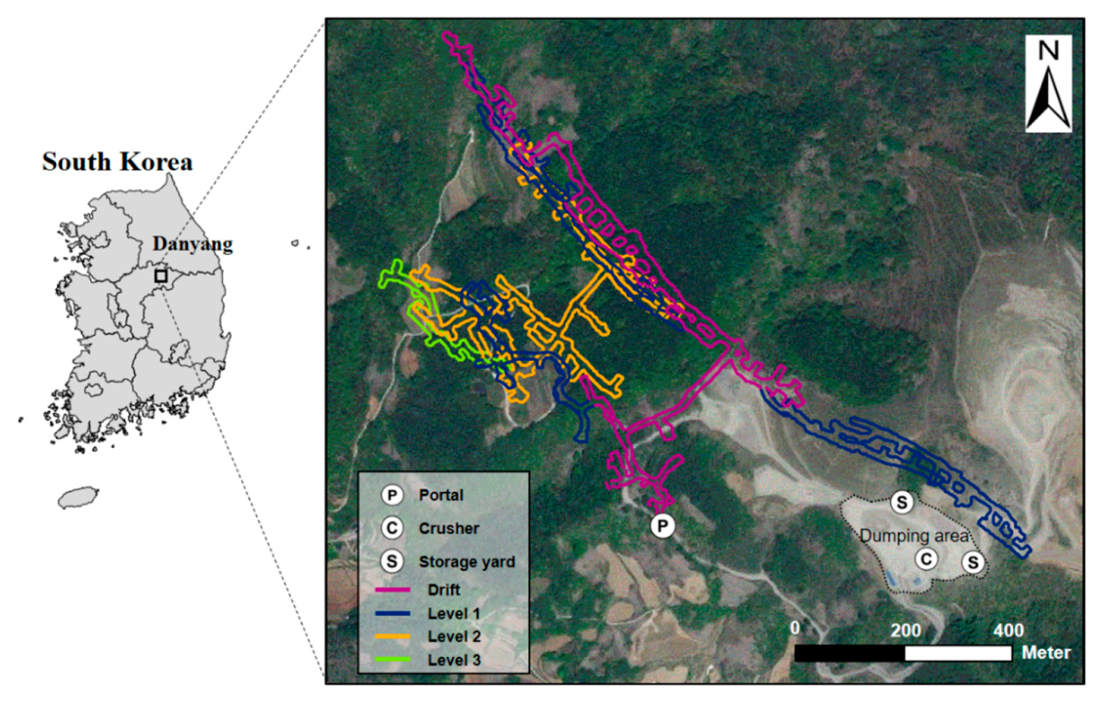
This study selected Baek Kwang Mineral Products Co., Ltd.’s Yeongcheon underground mine (37°4′14″, 128°18′46″) located in the city of Danyang in the Chungcheong province of South Korea as the study area. This mine produces 1.2 million tons of high-grade limestone ore annually through a room and pillar mining method. Figure 1 shows the arrangement of the five operation sites, which consist of a drift and three levels, and the location of the outdoor crushing sites. The drift’s average altitude above sea level is 313.4 m, and the lowermost level’s (Level 3) average altitude above sea level is 221.6 m.
At the Yeongcheon mine, 30-ton trucks travel back and forth between the loading sites and outdoor crushing sites to haul the ore. Production operation managers analyze ore production amounts, dispatch dump trucks in real time, and inform truck drivers of their destinations. The truck drivers follow haulage paths and travel to the loading sites located within the mine. The loaders that are waiting at the loading sites load the ore into the dump trucks. The dump trucks move to the outdoor crushing site, and the amount of ore that is piled in the crusher is checked. If this amount is below the limit capacity, the ore is dropped in the crusher. If the ore exceeds a fixed capacity, the ore is piled at an outdoor storage site. The truck that dropped off the ore receives another destination from a production operation manager and moves to the mine entrance.
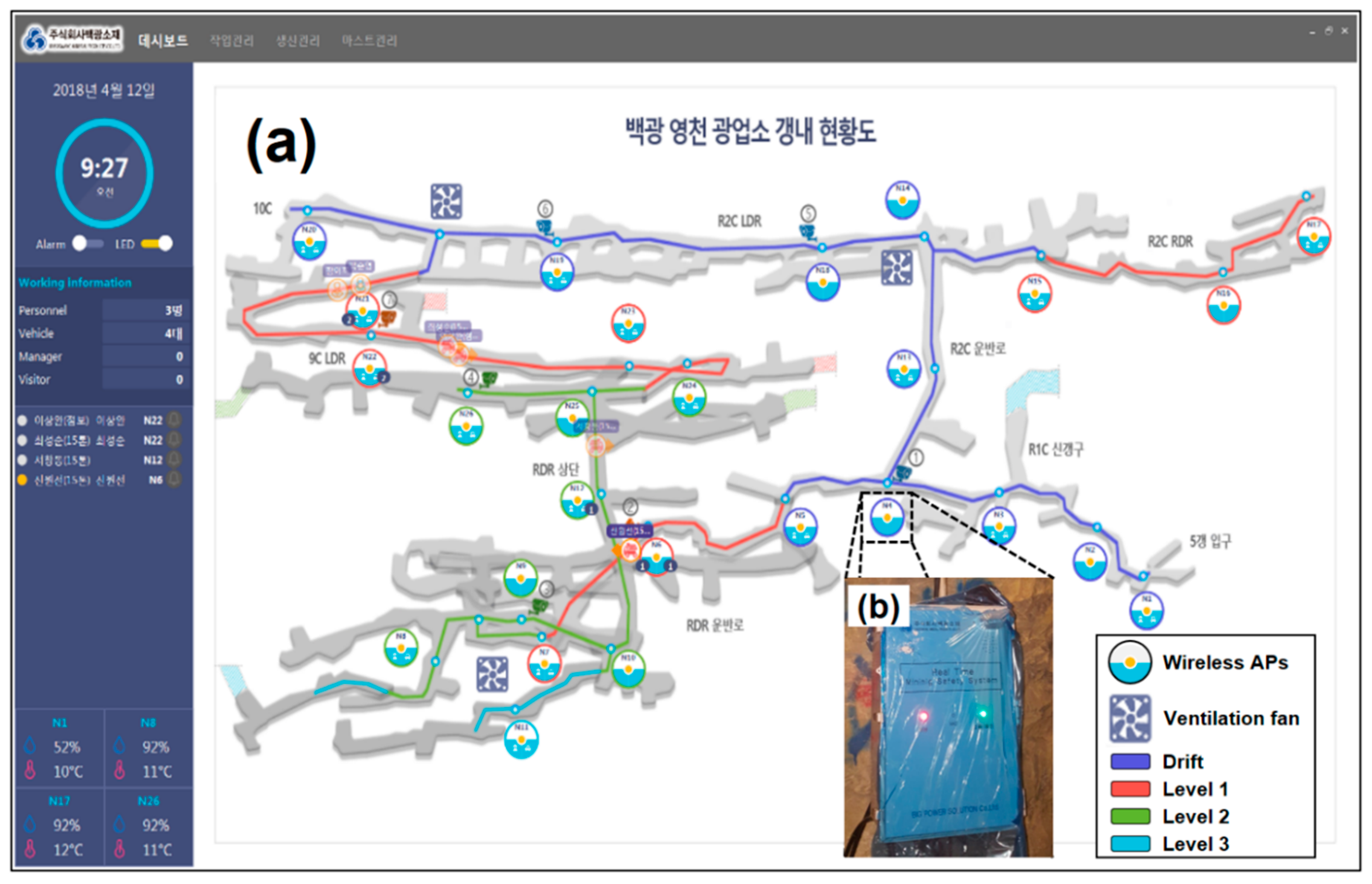
Figure 2 shows the components of the mine safety management system installed in the study area. To create the wireless communications network, 37 ultra-wideband (UWB) wireless APs were installed in the mine and three 900-MHz wireless APs were installed at the crushing site and the outdoor storage site outside the mine. Through the wireless communications network, the locations of the production equipment in the mine could be visualized in real time on the dashboard installed in the mine’s exterior office.
Table 1 shows the communication protocol format of the packet data acquired by the mine safety management system. The packet data can be classified as tag recognition data and environment monitoring data, and each types of data occupies 20 bytes. When packet data are transferred to the web server, they are preceded by the transmission date, time, and the IP address of the wireless AP that transmits the data. The communication protocol places STX and ETX, which indicate the packet’s start and end, at the front and end of the packet data. CHKSUM is included, which is the sum of all the values from after STX to before the check sum. Command packets include useful information acquired by the wireless APs. Tag recognition packet data include the data category, presence of an emergency situation, tag recognition sequence, recognized tag’s ID, and distance between the wireless AP and tag. The tag sequence consists of a number between 0 and 255, and it is incremented by 1 in 1 s. After 255, it changes back to 0. In other words, this value indicates the order of tag recognition and how much time has elapsed since the previous tag recognition occurred. As 15 tags were attached to the dump trucks and other equipment in the study area, it is essential to extract only the ID of the tag attached on the dump truck in tag recognition packet data to measure truck travel time.
The environment monitoring packet data include the data category, temperature, humidity, presence of earthquakes in the underground mine, presence of power supply equipment or battery use, battery level, and presence of the LED lights of wireless APs. Tag recognition packet data are transmitted once per second while the wireless AP recognizes the tag that is attached to the production equipment. During a single month, approximately 200,000 packets accumulate on the web server. Environment monitoring packet data are transmitted to the web server once every minute. Approximately 57,600 packets accumulate per day and approximately 173 million packets per month.
3. Methods
Truck travel time was measured using big data through the following process. First, only truck tag recognition packet data were extracted from the big data that accumulated on the web server. Then, the data were classified according to the number of truck haulage operations considering tag recognition time, wireless AP’s IP address, etc. Next, the differences in tag recognition times were calculated to obtain truck travel times according to the number of haulage operations. In this study, a truck haulage system simulation algorithm that uses measured truck travel times as input data was designed and a new program was developed for running the simulation.
3.1. Measuring Truck Travel Times from Big Data
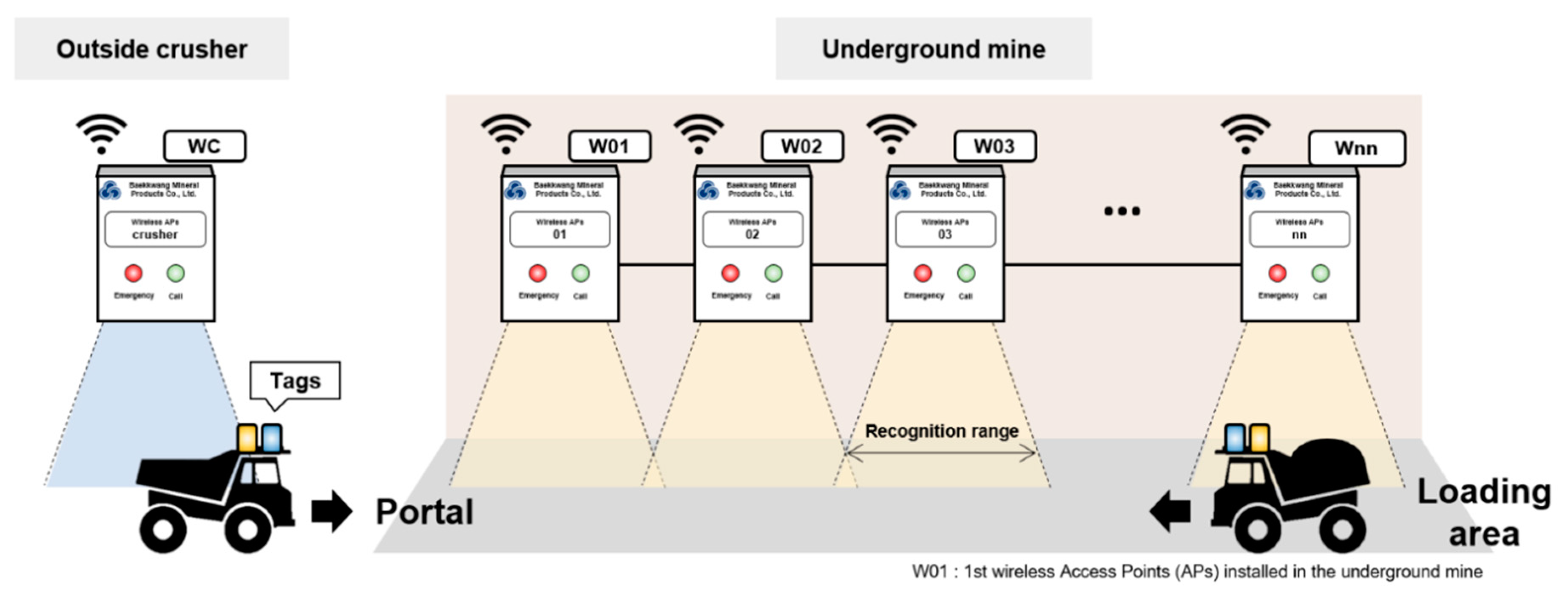
Only truck tag recognition packet data were extracted to consider only the temporal parameters required to measure truck travel times from big data. Then, the truck tag recognition packet data were classified according to the number of haulage operations. Figure 3 shows the features of the wireless APs that are passed while a truck is hauling ore in the underground mine.
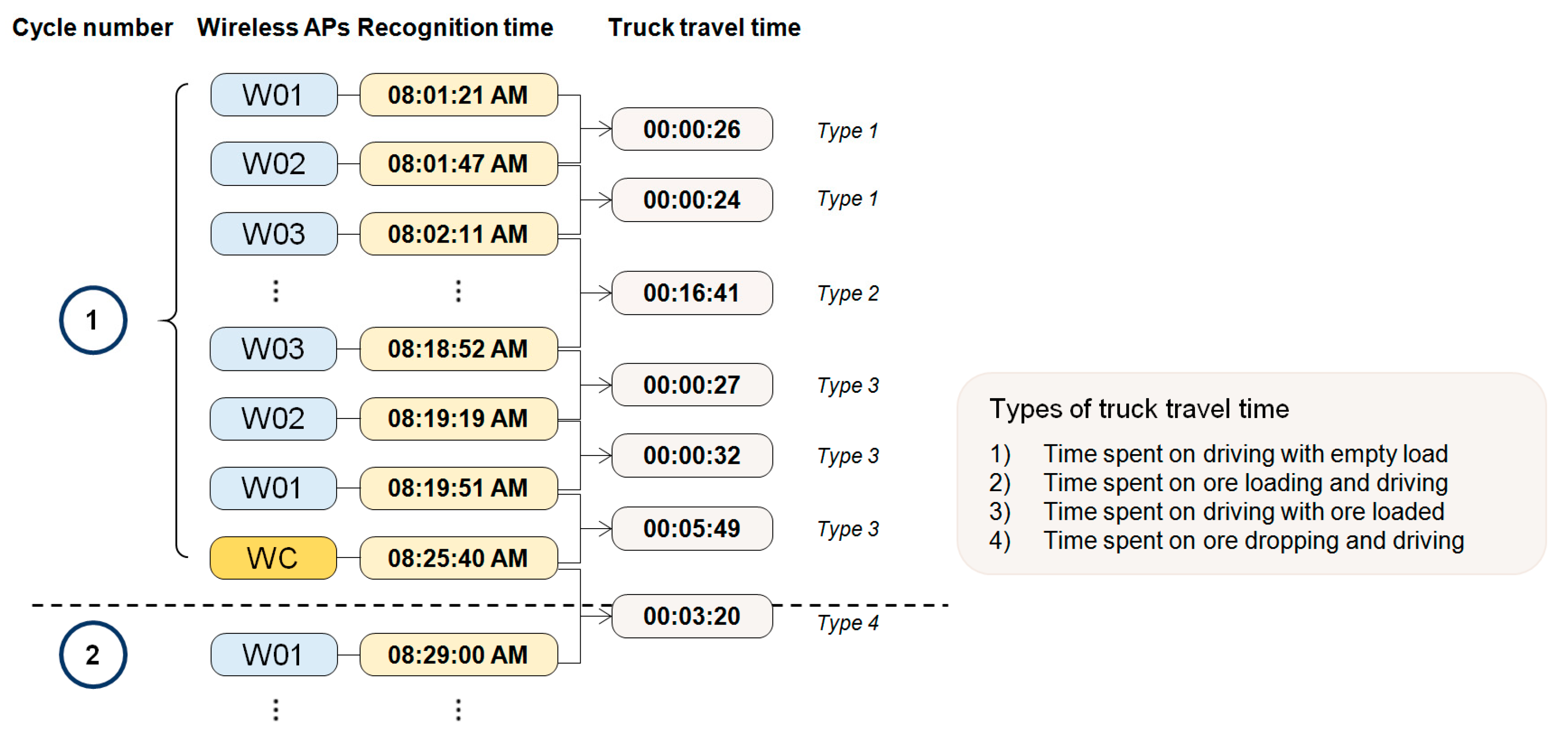
The last number in a wireless AP’s IP address is the same as the order in which the wireless AP was installed. W01 at the underground mine’s entrance was installed first, and therefore, the last number in its IP address is 1. The deeper the wireless AP is located within the mine, the larger the last number in its IP address. In other words, as a truck hauls ore, the last numbers in the IP addresses of wireless APs in the tag recognition data increase from 1 to the maximum and then decrease back down to 1. Therefore, the 1st wireless AP tag recognition time was searched for, and then, the 1st wireless AP tag recognition time was searched for again. The data that existed between the two time instances were classified as having occurred during the same haulage operation. The data that were classified according to the number of truck haulage operations were combined with the tag recognition packet data obtained from the crushing site (see Figure 4). When trucks loaded with ore travel away from W01 to the crushing site, the wireless AP installed at the crusher (WC) recognizes the trucks. When a truck drops the ore off in a hopper and then re-enters the portal of the underground mine to load ore, W01 recognizes the truck. The time at which WC recognizes the truck must be larger than the time at which W01 finally recognizes the truck in the previous haulage operation, and it must be less than the time at which W01 first recognizes the truck in the subsequent haulage operation. If this principle was satisfied, the data were combined. If not, it was determined that the time parameters for measuring truck travel times could not be extracted from the two data, and they were deleted.
To measure truck travel times, this study extracted the tag recognition times of all wireless APs from the data that were classified as having the same number of haulage operations. When a truck is stopped within a tag recognition range for a long time, the tag is continually recognized by a single wireless AP, and a large amount of tag recognition temporal data accumulate. In such cases, distance packet information was used to extract tag recognition time as the time when the distance between the wireless AP and truck was the minimum. The difference in tag recognition times was calculated, and truck travel time was measured. The four types of calculated truck travel times are as follows:
- the time during which a truck travels from one wireless AP to another;
- the time during which the truck is stopped at the loading site to load ore;
- the time during which the loaded truck travels from the mine entrance to the outdoor crushing site;
- the time during which the truck travels back to the mine entrance after finishing the ore drop-off operation at the crushing site.
A new program was developed to perform the time study. Only truck tag recognition packet data were extracted from the big data, and then, they were entered into the program in ASCII format. The program consists of a module that classifies truck tag packet data according to the number of haulage operations and a module that extracts tag recognition times and calculates truck travel times. When the calculations are complete, the truck travel time calculation results are produced in ASCII format (Table 2).
3.2. Truck Haulage Simulation
In this study, a discrete event simulation that can simulate the truck haulage system in the study area is developed. The simulation’s algorithm is based on the truck cycle time theory proposed by Suboleski [53]. In the truck cycle time theory, individual trucks’ operation times are expressed as in Equation (1):
where TCT is the truck cycle time; STL is the time during which a truck is accessed by the loading equipment; LT is the time during which the ore is loaded; TL is the time during which the loaded truck travels to the crushing site; STD is the time during which the truck is accessed by the crusher (outdoor storage site); DT is the time during which the ore is dropped off; TE is the time during which the truck travels to the loading site after performing the ore drop-off operation; AD is the time during which the truck waits during ore loading and drop-off.
TCT = STL + LT + TL + STD + DT + TE + AD
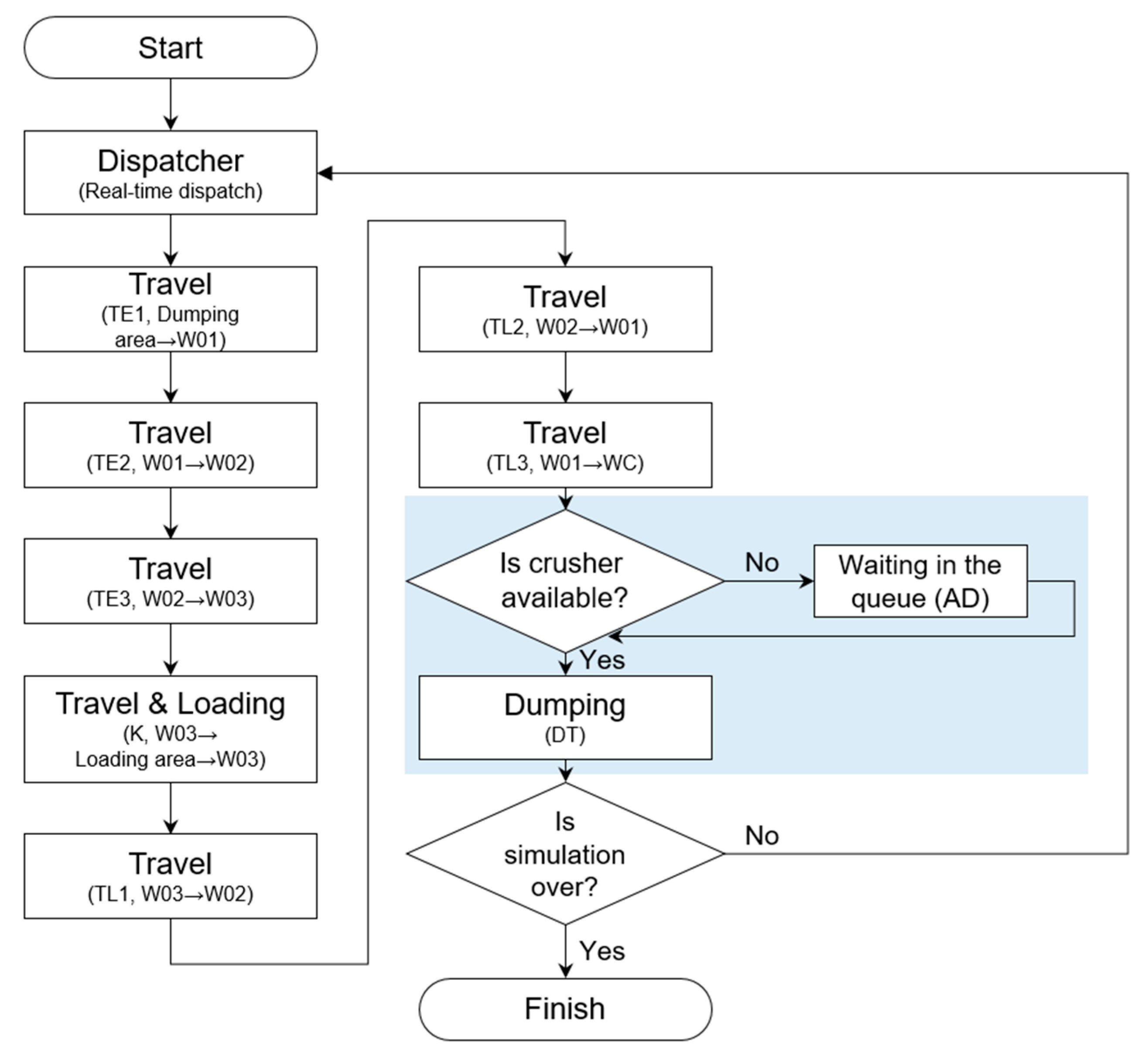
Figure 5 shows the algorithm of the truck haulage system simulation. When the simulation begins, a truck’s destination is assigned by a real-time dispatching method. The truck departs from the crushing site and travels to the W01 AP located at the mine entrance (TE1). Then, it travels to the W01-W02 segment (TE2) and W02-W03 segment (TE3). The truck travels toward the assigned destination from the crossroads located close to W03. It performs the ore loading operation and returns to W03 (K). Then, it travels to the W03-W02 segment (TL1) and W02-W01 segment (TL2), and it travels from the mine entrance to the WC located at the crushing site (TL3).
The truck that arrives at the crushing site checks whether there are trucks waiting to perform the ore drop-off operation. If there are trucks waiting, the truck waits until the waiting trucks complete the ore drop-off operation (AD). If there are no trucks waiting, the truck drops the ore off in the hopper (DT). This operation also includes cases where the truck travels to the outdoor storage site and drops the ore off if the amount of ore in the crusher hopper exceeds the limit capacity. The user-specified simulation end time and the simulation’s absolute time are compared to determine whether the truck will perform the loading operation again or whether the simulation will end.
The Windows-based truck haulage simulation program employed in this study consists of a graphical user interface (GUI) and a simulation engine. Through the GUI, a user can enter the simulation factors (operation days, daily operation time, number of trucks, truck weight, etc.) and temporal factors (truck operation time, ore drop-off time, etc.) that are required to run the simulation. Table 3 lists the input and output data of the program. The averages and standard deviations of the temporal factors are calculated through statistical analysis using the truck travel times for all haulage cycles obtained in Section 3.1. The simulation engine runs when the user finishes inputting the simulation factors and clicks the ‘Run’ button. The simulation results can be seen by clicking the ‘View’ button.
The simulation engine was developed based on GPSS/H, which is a typical simulation language. Please refer to Sturgul [54,55] for a detailed description of the GPSS/H language. The simulation engine performs three functions. First, it generates the simulation’s input data based on the simulation factors and time factors entered by the user in the GUI. Next, it uses the generated input data to run the simulation and produces the results in a text file format. The produced simulation results include the total simulation running time, total amount of hauled ore, crusher utilization, and the time that trucks spent waiting at the crushing site. When the simulation finishes running, the simulation results are visualized in the program GUI.
4. Results
Big data were collected for three months, from October 1 to December 31, 2018. The overall number of packet data was 7,065,591. Of these, the number of truck tag recognition packet data was 808,130. Only tag recognition packet data were extracted from the big data, and they were classified according to the number of truck haulage operations. Table 4 shows the tag IDs for the UWB and 900 MHz tags attached to the 4 trucks that performed haulage operations in the study area, and it shows the number of haulage operations performed by each truck. The number of haulage operations performed by the 4 trucks was 579, which was comprised of 268, 277, and 34 operations performed in October, November, and December, respectively. When the number of haulage operations was found to be 0, it was because the truck performed haulage operations at a different operation site during that month.
To measure truck travel time, this study extracted the times at which the wireless APs recognized the tags for each number of haulage operations, and then, it calculated their differences. However, as measured truck travel times include the times that occur as exceptions, such as meals and excessive waits, it was necessary to remove the abnormal values that deviated considerably from the average. In this study, the average and standard deviation were calculated for each unit of travel time. The data that exceeded the mean value by more than three standard deviations were considered to be abnormal values and removed. The cumulative relative frequency of the data was calculated, and the values with a cumulative relative frequency of less than 0.05 or larger than 0.95 were deleted.
Table 5 shows the results of using statistical analysis to calculate the quantity, average, and standard deviation of measured truck unit travel time data. Regarding the time during which a truck left W03 and performed the load operation and then returned to W03, two data sets (K1, K2) were classified according to the distance to the loading site. K1 is the case in which a truck travels from W03 to a relatively close loading site, and K2 is the case in which a truck travels from W03 to a long-distance loading site. There were relatively fewer data for the TE1 time compared with other times because the TE1 times could not be obtained as there were no times at which the crushing site wireless APs recognized the truck tags during the beginning of the day’s first haulage operations.
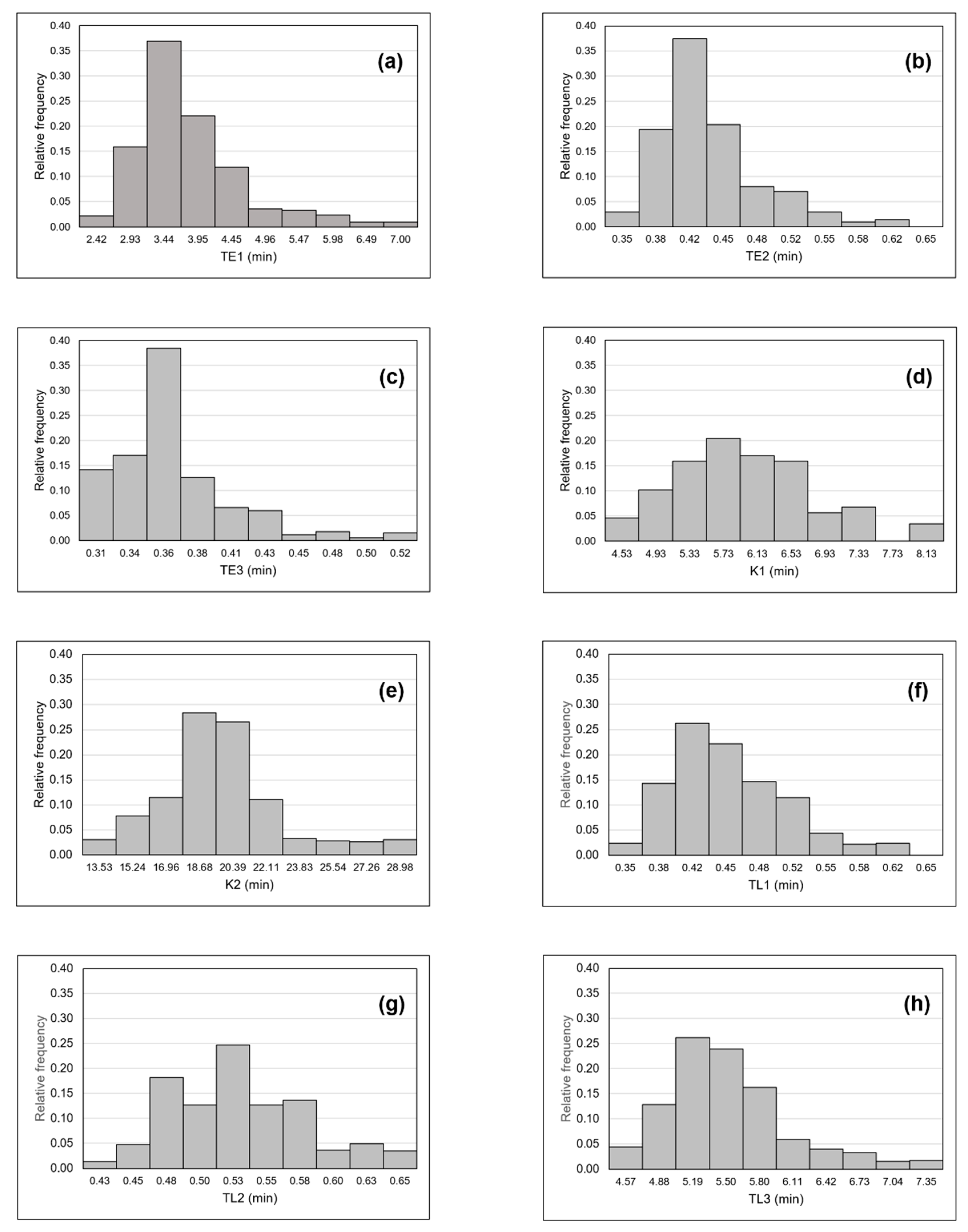
Figure 6 shows histograms for truck unit travel time data. All truck travel time data are shown in the form of a normal distribution. The GPSS/H simulation codes were modified to obtain the time spent on each unit operation according to a normal distribution in the simulation. In the simulation, the probability that a truck will travel for K1 and K2 times was set as 17% and 83%, respectively, according to the ratio of the number of data in K1 and K2 that occurred over the three months.
The calculated averages and standard deviations of truck travel times were entered as time factors, and the truck haulage system simulation was performed. To verify the simulation, the simulation factors were set to be the same as the haulage operation environment on January 2 and 9, 2019. Following the haulage operation records for January 2, 2019, the simulation was performed by setting the total simulation time as 1 day, the daily operational time as 6 h and 50 min (400 min), the number of trucks as 1, and the truck loading capacity as 30 tons. Following the haulage operation records for January 9, 2019, the simulation was performed by setting the total simulation time as 1 day, the daily operational time as 5 h (300 min), the number of trucks as 1, and the truck loading capacity as 30 tons.
After ore loading operations, a loaded truck exits the mine and arrives at the crushing area, drops off ore, and then re-enters the mine. At this time, the W01-WC-W01 wireless APs continuously recognize the tags attached on the truck, and the TL3 time and TE1 time can be measured by calculating the difference between tag recognition times. The calculated TE1 time also includes the time spent on ore dumping. However, there was a limit to extracting exact dumping time through the wireless AP system installed in the study area. Thus, it was assumed that the time during which trucks dropped off ore was the same in all underground mines, and a time of 0.59 ± 0.11 min was used, which was measured by Choi et al. [45] using a stopwatch.
Table 6 shows a comparison of the simulation results and actual haulage operation records. On January 2, the predicted and actual number of times that trucks dropped off ore were 13 and 12, respectively. However, the time during which trucks waited at the crushing site did not occur in either of the results. On January 9, the predicted and actual results for the number of ore loads, loaded ore’s weight, and loading wait times were the same. However, there was a difference of 1 in the number of occurrences of K1 time and K2 time.
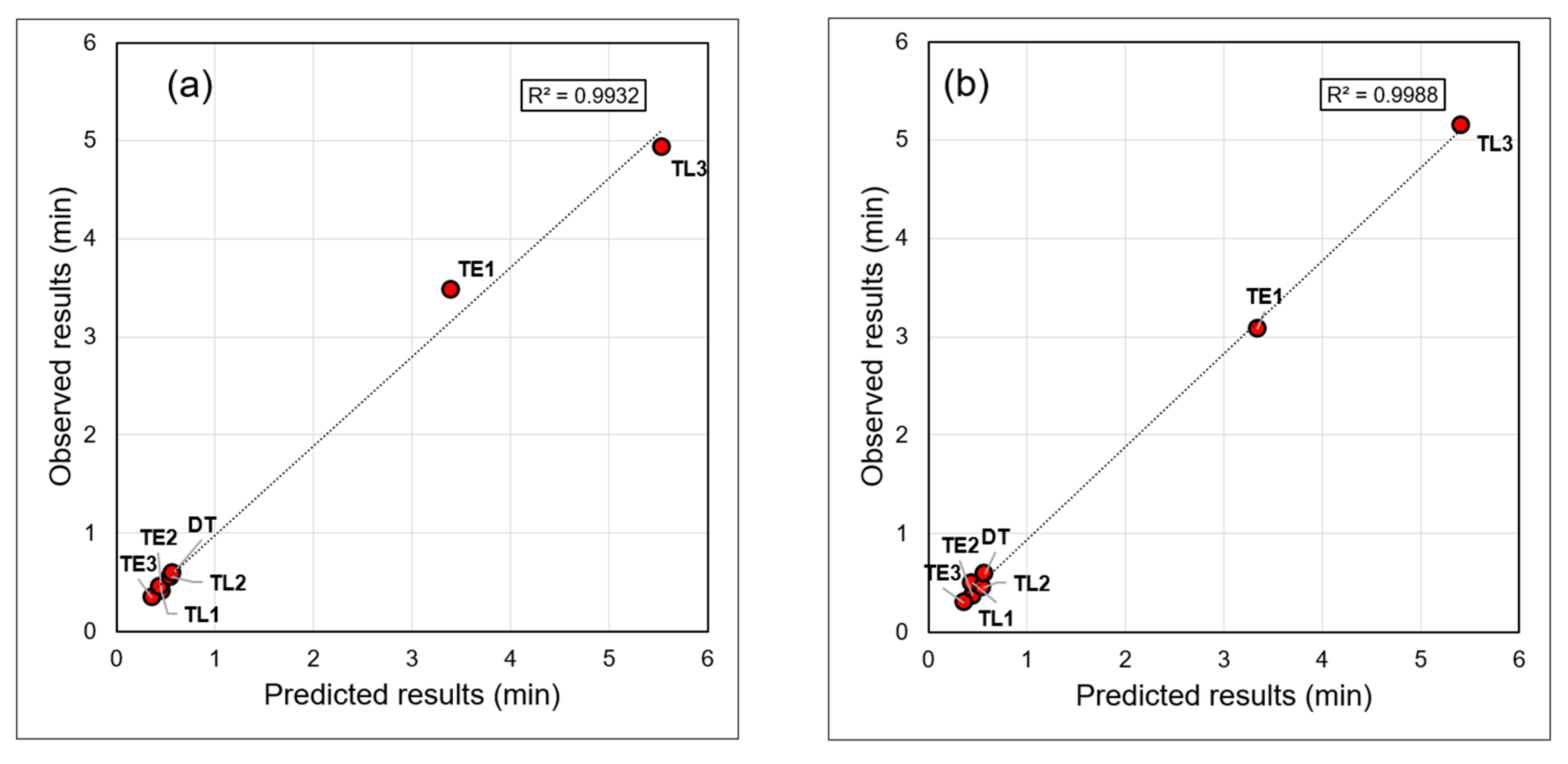
Figure 7 presents the correlation between the mean truck travel times derived from the simulation results and the actual truck haulage operation results.
In both cases, the coefficient of determination is 0.99, which suggests that there is a high correlation between the predicted and observed mean truck travel times. After calculating the mean and standard deviation of the truck travel times measured from the simulation results and the actual truck haulage operation results, the absolute error between the two results was calculated (see Table 7). The mean absolute errors between the predicted and observed truck travel times were 0.13 min for January 2 and 0.14 min for January 9. It was found that the truck unit haulage operation times obtained through the simulation were almost the same as the time spent during actual haulage operations.
5. Discussion
5.1. Measurement of Truck Travel Time by Setting Different Tag Recognition Data Aggregation Periods
The changes in truck travel time statistics that occurred when the data aggregation period was set differently were analyzed in this study. The analyses focused on the tag recognition packet data acquired from October to December, 2018. The data aggregation period was set as the most recent day (2018/12/28), 5 days (2018/12/24–2018/12/28), 10 days (2018/12/17–2018/12/28), 1 month (2018/12), 2 months (2018/11–2018/12), and 3 months (2018/10–2018/12). Table 8 shows the statistical values of truck unit travel time that were found when the data aggregation period was set differently. DT was assumed to be constant even when the data aggregation period changed. TE1, TE2, TE3, TL1, TL2, and TL3 maintained relatively fixed times even as the period changed. Therefore, it is possible to calculate statistical values for these times using data collected during a short period.
The statistical values for K1 could not be calculated for the last 1 day, 5 days, 10 days, or one month and could only be calculated for October and November because data collection was not performed for December. Therefore, to calculate accurate statistical values for the K1 time, it is necessary to use the data obtained over a long period. It is known that large fluctuations occur in the K2 time in the statistical results acquired during a period of less than one month. In other words, similar to the K1 time, the statistical values for the K2 time must be calculated using the data acquired over a long period.
5.2. Comparison of Truck Haulage Simulation Results Using Different Truck Travel Times
The truck travel times that were measured differently according to the data aggregation period were set as temporal factors, and truck haulage simulations were performed. The simulation setting factors were set to be the same as the haulage operation environment on January 9, 2019. Table 9 shows a comparison of the simulation results and the haulage operation results from January 9, 2019. In a comparison of the actual haulage operation results and the simulation results obtained using the data collected during a period of less than 1 month, the K1 time did not occur in both results, but there was a relatively large difference in the occurrence of the K2 time. Moreover, it was found that ore production amounts did not accurately match during the period, except for the last day.
In a comparison of the actual haulage operation results and the simulation results obtained using the data collected during a period of more than two months, there were relatively small differences in truck travel times, except for the K1 time. The ore production amounts between the simulation results and actual operation results were in good agreement, but the number of times that K1 and K2 occurred was different. This is because the probability that the K1 time and K2 time will occur in the discrete event simulation was set as 17% and 83%, respectively. However, in case of the actual haulage operation, trucks may drive only the longest haulage road to load the ore. When haulage simulations were performed using the data acquired over a long period, the overall truck travel time and production amount could be predicted accurately. More accurate simulation results can be achieved if the number of times that a truck visits the loading site can be reflected in the simulation beforehand by performing haulage operation planning.
6. Conclusions
In this work, the temporal factors of truck tag recognition were extracted from the big data acquired through an underground mine safety management system, and a time study was performed to measure truck travel times. Additionally, a discrete event simulation that could simulate the truck haulage system of an underground limestone mine was designed, and a Windows-based simulation program for was developed running the simulation. Statistical analysis was performed using the big data acquired in October, November, and December 2018 to calculate the averages and standard deviations of the time spent on each truck unit operation during 579 truck haulage operations. The statistical values of truck travel time were used to perform a truck haulage simulation, and the results were compared with the results of actual haulage operations performed on January 2 and 9, 2019. The difference between the predicted and observed results for the total amounts of loaded ore was 30 tons and 0 tons on January 2 and 9, respectively. Moreover, the mean absolute errors between the predicted and observed mean truck travel times were 0.13 min and 0.14 min on January 2 and 9, respectively. This comparison showed that the developed truck haulage simulation could predict truck ore load, total ore production amounts, and truck wait times, which were in good agreement with actual values.
Tag recognition packet data were extracted from the big data by setting the data aggregation period as 1 day, 5 days, 10 days, 1 month, 2 months, and 3 months, and then, truck travel times were measured. The results showed that accurate travel time measurements were possible when using the data that had been collected over a long period. Further, accurate simulation results were produced when the statistical values of truck travel time obtained from long-term data were entered in the simulation. Accurate travel time measurements are possible when using the big data that have been collected on a web server over a long time by a mine safety management system. Further, specific simulation designs and accurate simulation results can be produced because the long-term cumulative time factors for various truck haulage paths can be extracted from big data.
In this study, the probability that the K1 time and K2 time will occur in the discrete event simulation was set to be the same as the ratio of the quantity of data for which the two times occurred during a certain period. For this reason, a problem occurred in which the number of occurrences of the K1 and K2 times was not the same in the actual haulage operation results and simulation results. If a haulage operation manager can accurately plan the number of visits to the loading site beforehand, the number of occurrences of the K1 and K2 times can be set as simulation factors, and accurate simulations can be performed. In addition, truck travel times are currently classified only by the K1 and K2 times according to the distance from W03 to the loading site. If truck travel times are divided into multiple times based on the number of loading sites when the simulations are performed, it is possible achieve better agreement between predicted and actual haulage operation results.
In future, we plan to develop a truck haulage simulation algorithm that can consider the various truck delay times that occur when a truck stops driving. In an actual haulage operation, there are various types of truck delay times, such as the time required for an empty truck to yield a loaded truck on a narrow underground haulage road and the time of waiting for an order of ore loading. Therefore, it is necessary to identify the types of truck delay times and the locations where the delay times occur in the study area. Considering these conditions, the existing truck haulage simulation algorithm, neural networks, and mathematical programming methods should be updated.
Author Contributions
Y.C. conceived and designed the experiments; J.B. performed the experiments; J.B. and Y.C. analyzed the data; Y.C. contributed reagents/materials/analysis tools; J.B. and Y.C. wrote the paper.
Funding
This work was supported by Institute for Information & communications Technology Promotion (IITP) grant funded by the Korea Government’s Ministry of Science and ICT (Project No. 2018-0-01282).
Conflicts of Interest
The authors declare no conflict of interest.
References
- Centers for Disease Control and Prevention (CDC). Number and Rate of Occupational Mining Fatalities by Year, 2008–2017. Available online: https://wwwn.cdc.gov/niosh-mining/MMWC/Fatality/NumberAndRate (accessed on 10 June 2019).
- Yarkan, S.; Sabih, G.; Murphy, R.R. Underground Mine Communications: A Survey. IEEE Commun. Surv. Tutor. 2009, 11, 125–142. [Google Scholar] [CrossRef]
- Sunderman, C.; Waynert, J. An Overview of Underground Coal Miner Electronic Tracking System Technologies. In Proceedings of the 2012 IEEE Industry Applications Society Annual Meeting, Las Vegas, NV, USA, 7–11 October 2012; IEEE: New York, NY, USA, 2012; pp. 1–5. [Google Scholar]
- Forooshani, A.E.; Bashir, S.; Michelson, D.G.; Noghanian, S. A Survey of Wireless Communications and Propagation Modeling in Underground Mines. IEEE Commun. Surv. Tutor. 2013, 15, 1524–1545. [Google Scholar] [CrossRef]
- Dohare, Y.S.; Maity, T.; Das, P.S.; Paul, P.S. Wireless Communication and Environment Monitoring in Underground Coal Mines—Review. IETE Tech. Rev. 2015, 32, 140–150. [Google Scholar] [CrossRef]
- Thrybom, L.; Neander, J.; Hansen, E.; Landernäs, K. Future Challenges of Positioning in Underground Mines Future Challenges of Positioning in Underground Mines. IFAC Pap. 2015, 48, 222–226. [Google Scholar] [CrossRef]
- Reddy, N.S.; Saketh, M.S.; Dhar, S. Review of Sensor Technology for Mine Safety Monitoring Systems: A Holistic Approach. In Proceedings of the 2016 IEEE First International Conference on Control, Measurement and Instrumentation (CMI), Kolkata, India, 8–10 January 2016; IEEE: New York, NY, USA, 2016; pp. 429–434. [Google Scholar]
- Muduli, L.; Mishra, D.P.; Jana, P.K. Application of Wireless Sensor Network for Environmental Monitoring in Underground Coal Mines: A systematic review. J. Netw. Comput. Appl. 2018, 106, 48–67. [Google Scholar] [CrossRef]
- Wu, Y.; Chen, M.; Wang, K.; Fu, G. A Dynamic Information Platform for Underground Coal Mine Safety based on Internet of Things. Saf. Sci. 2019, 113, 9–18. [Google Scholar] [CrossRef]
- Bandyopadhyay, L.K.; Chaulya, S.K.; Mishra, P.K.; Choure, A.; Baveja, B.M. Wireless Information and Safety System for Mines. J. Sci. Ind. Res. India 2009, 68, 107–117. [Google Scholar] [CrossRef]
- Wei, S.; Li-li, L. Multi-parameter Monitoring System for Coal Mine based on Wireless Sensor Network Technology. In Proceedings of the 2009 International Conference on Industrial Mechatronics and Automation, Chengdu, China, 15–16 May 2009; Luo, Q., Zhou, Q., Eds.; IEEE: New York, NY, USA, 2009; pp. 225–227. [Google Scholar]
- Chehri, A.; Farjow, W.; Mouftah, H.T.; Femando, X. Design of Wireless Sensor Network for Mine Safety Monitoring. In Proceedings of the 2011 24th Canadian Conference on Electrical and Computer Engineering(CCECE), Niagara Falls, ON, Canada, 8–11 May 2011; IEEE: New York, NY, USA, 2011; pp. 001532–001535. [Google Scholar]
- Xu, X.; Zheng, P.; Li, L.; Chen, H.; Ye, J.; Wang, J. Design of Underground Miner Positioning System Based on ZigBee Techonology. In Proceedings of the International Conference on Web Information Systems and Mining, Chengdu, China, 26–28 October 2012; Wang, F.L., Lei, J., Gong, Z., Luo, X., Eds.; Springer: Berlin, Germany, 2012; pp. 342–349. [Google Scholar]
- Zhang, Y.; Yang, W.; Han, D.; Kim, Y. An Integrated Environment Monitoring System for Underground Coal Mines-Wireless Sensor Network Subsystem with Multi-Parameter Monitoring. Sensors 2014, 14, 13149–13170. [Google Scholar] [CrossRef]
- Moridi, M.A.; Kawamura, Y.; Sharifzadeh, M.; Chanda, E.K.; Jang, H. An Investigation of Underground Monitoring and Communication System Based on Radio Waves Attenuation Using ZigBee. Tunn. Undergr. Space Technol. 2014, 43, 362–369. [Google Scholar] [CrossRef]
- Moridi, M.A.; Kawamura, Y.; Sharifzadeh, M.; Chanda, E.K.; Wagner, M.; Jang, H.; Okawa, H. Development of Underground Mine Monitoring and Communication System Integrated ZigBee and GIS. Int. J. Min. Sci. Technol. 2015, 25, 811–818. [Google Scholar] [CrossRef]
- Nithya, T.; Ezak, M.M.; Kumar, K.R.; Vignesh, V.; Vimala, D. Rescue and Protection System for Underground Mine Workers Based On ZIGBEE. Int. J. Recent Res. Asp. 2018, 4, 194–197. [Google Scholar]
- Moridi, M.A.; Kawamura, Y.; Sharifzadeh, M.; Knox, E.; Wagner, M.; Okawa, H. Performance Analysis of ZigBee Network Topologies for Underground space monitoring and communication systems. Tunn. Undergr. Space Technol. 2018, 71, 201–209. [Google Scholar] [CrossRef]
- Bai, M.; Zhao, X.; Hou, Z.; Tan, M. A Wireless Sensor Network Used in Coal Mines. In Proceedings of the 2007 IEEE International Conference on Networking, Sensing and Control, London, UK, 15–17 April 2007; IEEE: New York, NY, USA, 2007; pp. 319–323. [Google Scholar]
- Chen, G.; Zhu, Z.; Zhou, G.; Shen, C.; Sun, Y. Sensor Deployment Strategy for Chain-type Wireless Underground Mine Sensor Network. J. China Univ. Min. Technol. 2008, 18, 0561–0566. [Google Scholar] [CrossRef]
- Liu, Z.; Li, C.; Wu, D.; Dai, W.; Geng, S.; Ding, Q. A Wireless Sensor Network Based Personnel Positioning Scheme in Coal Mines with Blind Areas. Sensors 2010, 10, 9891–9918. [Google Scholar] [CrossRef] [PubMed]
- Xu, H.; Li, F.; Ma, Y. A ZigBee-based miner Localization System. In Proceedings of the 2012 IEEE 16th International Conference on Computer Supported Cooperative Work in Design (CSCWD), Wuhan, China, 23–25 May 2012; IEEE: New York, NY, USA, 2012; pp. 919–924. [Google Scholar]
- Bhattacharjee, S.; Roy, P.; Ghosh, S.; Misra, S.; Obaidat, M.S. Wireless sensor network-based fire detection, alarming, monitoring and prevention system for Bord-and-Pillar coal mines. J. Syst. Softw. 2012, 85, 571–581. [Google Scholar] [CrossRef]
- Cheng, G. Accurate TOA-Based UWB Localization System in Coal Mine Based on WSN. Phys. Procedia 2012, 24, 534–540. [Google Scholar] [CrossRef] [Green Version]
- Guo, P.; Jiang, T.; Zhang, K. Novel Energy-Efficient MinerMonitoring System with Duty-CycledWireless Sensor Networks. Int. J. Distrib. Sens. Netw. 2012, 8, 1–9. [Google Scholar] [CrossRef]
- Mahdavipour, O.; Mueller-sim, T.; Fahimi, D.; Croshere, S.; Pillatsch, P.; Merukh, J.; Baruffa, V.Z.; Sabino, J.; Tran, K.; Alanis, G.; et al. Wireless Sensors for Automated Control of Total Incombustible Content (TIC) of Dust Deposited in Underground Coal Mines. In Proceedings of the 2015 IEEE SENSORS, Busan, Korea, 1–4 November 2015; IEEE: New York, NY, USA, 2015; pp. 1–4. [Google Scholar]
- Mine Site Technologies’ IMPACT. Available online: http://mstglobal.com/wp-content/uploads/2014/11/MST-ICA-Overview-Overview.pdf (accessed on 3 April 2019).
- Strata Worldwide’s STRATACONNECT™. Available online: https://www.strataworldwide.com/sites/default/files/platform//brochure/StrataConn_A4-Broch-2016.pdf (accessed on 3 April 2019).
- Becker Mining Systems’ MineView. Available online: https://www.becker-mining.com/sites/default/files/uploads/ProductBrochures/BMS_MineView_Brochure_web.pdf (accessed on 3 April 2019).
- ORBCOMM’s Real-Time Location System (RTLS). Available online: https://www.orbcomm.com/en/solutions/web-applications/assetwatch-mining (accessed on 3 April 2019).
- McKinsey & Company. Big Data: The Next Frontier for Innovation, Competition, and Productivity. Available online: https://www.mckinsey.com/business-functions/digital-mckinsey/our-insights/big-data-the-next-frontier-for-innovation (accessed on 10 June 2019).
- World Economic Forum. Big Data, Big Impact: New Possibilities for International Development. Available online: http://www3.weforum.org/docs/WEF_TC_MFS_BigDataBigImpact_Briefing_2012.pdf (accessed on 10 June 2019).
- IBM. Analytics: The Real-World Use of Big Data. Available online: http://www.informationweek.com/pdf_whitepapers/approved/1372892704_analytics_the_real_world_use_of_big_data.pdf (accessed on 10 June 2019).
- IBM. IBM and Goldcorp Team to Bring Watson to the Mines. Available online: https://www.ibm.com/news/ca/en/2017/03/03/t817903u78442c90.html (accessed on 17 April 2019).
- Mining.com. Goldcorp Partners with IBM to Hunt for Exploration Targets at Red Lake. Available online: http://www.mining.com/goldcorp-partners-ibm-hunt-exploration-targets-red-lake/ (accessed on 17 April 2019).
- NEWTRAX. Newtrax Partners with World-Leading AI Research Center to Discover New Insights in Underground Hard Rock Mines. Available online: https://www.newtrax.com/artificial-intelligence-montreal/ (accessed on 17 April 2019).
- Mining Magazine. The Future of Mining Is Underground. Available online: https://www.miningmagazine.com/partners/partner-content/1332132/the-future-of-mining-is-underground (accessed on 17 April 2019).
- Salama, A.; Greberg, J. Optimization of Truck-Loader haulage system in an underground mine: A simulation approach using SimMine. In Proceedings of the MassMin 2012: 6th International Conference & Exhibition on Mass Mining, Sudbury, ON, Canada, 10–14 June 2012; Canadian Institute of Mining, Metallurgy and Petroleum: Sudbury, ON, Canada, 2012. [Google Scholar]
- Saayman, F.R.; Craig, I.K.; Camisani-Calzolari, F.R. Optimization of an Autonomous Vehicle Dispatch System in an Underground Mine. J. Souther African Inst. Min. Metall. 2006, 106, 77–86. [Google Scholar]
- Roberts, B.H. Computer Simulation of Underground Truck Haulage Operations. Min. Technol. 2002, 111, 123–128. [Google Scholar] [CrossRef]
- Pop-Andonov, G.; Mirakovski, D.; Despotov, Z. Simulation Modeling and Analyzing in Underground Haulage Systems with ARENA Simulation Software. Int. J. Sci. Tecnol. Innov. Ind. MTM Mach. Tecnol. Mater. 2012, 11, 48–50. [Google Scholar]
- Fioroni, M.M.; dos Santos, L.C.A.; Franzese, L.A.G.; Santana, I.R.; Telles, G.D.; Seixas, J.C.; Penna, B.; de Alkmim, G.M. Logistic Evaluation of an Underground Mine Using Simulation. In Proceedings of the 2014 Winter Simulation Conference, Savannah, GA, USA, 7–10 December 2014; Tolk, A., Yilmaz, L., Diallo, S.Y., Ryzhov, I.O., Eds.; IEEE: New York, NY, USA, 2014; pp. 1855–1865. [Google Scholar]
- Park, S.; Choi, Y.; Park, H. Simulation of Truck-Loader Haulage Systems in an Underground Mine Using GPSS/H. Tunn. Undergr. Space 2014, 24, 430–439. [Google Scholar] [CrossRef]
- Park, S.; Choi, Y.; Park, H. Optimization of Truck-loader Haulage Systems in an Underground Mine Using Simulation Methods. Geosyst. Eng. 2016, 19, 222–231. [Google Scholar] [CrossRef]
- Choi, Y.; Park, S.; Lee, S.; Baek, J.; Jung, J.; Park, H. Development of a Windows-based Program for Discrete Event Simulation of Truck-Loader Haulage Systems in an Underground Mine. Tunn. Undergr. Space 2016, 26, 87–99. [Google Scholar] [CrossRef]
- Nehring, M.; Topal, E.; Knights, P. Dynamic Short Term Production Scheduling and Machine Allocation in Underground Mining Using Mathematical Programming. Min. Technol. 2010, 119, 212–220. [Google Scholar] [CrossRef]
- Gamache, M.; Grimard, R.; Cohen, P. A Shortest-path Algorithm for Solving the Fleet Management Problem in Underground Mines. Eur. J. Oper. Res. 2005, 166, 497–506. [Google Scholar] [CrossRef]
- Beaulieu, M.; Gamache, M. An Enumeration Algorithm for Solving the Fleet Management Problem in Underground Mines. Comput. Oper. Res. 2006, 33, 1606–1624. [Google Scholar] [CrossRef]
- Baek, J.; Choi, Y.; Lee, C.; Suh, J.; Lee, S. BBUNS: Bluetooth Beacon-Based Underground Navigation System to Support Mine Haulage Operations. Minerals 2017, 7, 228. [Google Scholar] [CrossRef]
- Jung, J.; Choi, Y. Collecting Travel Time Data of Mine Equipments in an Underground Mine Using Reverse RFID Systems. Tunn. Undergr. Space 2016, 26, 253–265. [Google Scholar] [CrossRef]
- Jung, J.; Choi, Y. Measuring Transport Time of Mine Equipment in and Underground Mine Using a Bluetooth Beacon System. Minerals 2017, 7, 1. [Google Scholar] [CrossRef]
- Baek, J.; Choi, Y.; Lee, C.; Jung, J. Performance Comparison of Bluetooth Beacon and Reverse RFID Systems as Potential Tools for Measuring Truck Travel Time in Open-Pit Mines: A Simulation Experiment. Geosyst. Eng. 2017, 21, 43–52. [Google Scholar] [CrossRef]
- Suboleski, S.C. Mine Systems Engineering Lecture Notes; The Pennsylvania State University: State College, PA, USA, 1975. [Google Scholar]
- Sturgul, J.R. Mine Design: Examples Using Simulation; Society for Mining, Metallurgy and Exploration (SME): Littleton, CA, USA, 2000; pp. 1–367. ISBN 9780873351812. [Google Scholar]
- Sturgul, J.R. Discrete Simulation and Animation for Mining Engineers, 1st ed.; CRC Press: Boca Raton, FL, USA, 2015; pp. 1–600. ISBN 978-1-4822-5442-6. [Google Scholar]
Figure 1.
Aerial view of the study area showing drifts inside the mine and outside facilities. (Image source: National Geographic Information Institute of South Korea).
Figure 1.
Aerial view of the study area showing drifts inside the mine and outside facilities. (Image source: National Geographic Information Institute of South Korea).

Figure 2.
Components of the mine safety management system installed in the study area: (a) main dashboard showing the location of dump trucks and loaders; (b) wireless APs.
Figure 2.
Components of the mine safety management system installed in the study area: (a) main dashboard showing the location of dump trucks and loaders; (b) wireless APs.

Figure 3.
Diagram showing the sequence of wireless APs in the underground mine.

Figure 4.
Diagram showing the process of classifying the truck tag recognition packet data according to the number of the haulage operation cycle, combining the data with the tag recognition packet data obtained from the crushing site, and measuring the 4 types of truck travel time.
Figure 4.
Diagram showing the process of classifying the truck tag recognition packet data according to the number of the haulage operation cycle, combining the data with the tag recognition packet data obtained from the crushing site, and measuring the 4 types of truck travel time.

Figure 5.
Flow chart showing procedures for implementing the truck haulage simulation algorithm.

Figure 6.
Histogram of the truck unit travel time data: (a) TE1; (b) TE2; (c) TE3; (d) K1; (e) K2; (f) TL1; (g) TL2; (h) TL3
Figure 6.
Histogram of the truck unit travel time data: (a) TE1; (b) TE2; (c) TE3; (d) K1; (e) K2; (f) TL1; (g) TL2; (h) TL3

Figure 7.
Results of correlation analysis between the predicted and observed mean truck travel times derived from the haulage operation results performed on (a) 2019-01-02 and (b) 2019-01-09.
Figure 7.
Results of correlation analysis between the predicted and observed mean truck travel times derived from the haulage operation results performed on (a) 2019-01-02 and (b) 2019-01-09.


Table 1.
Communication protocol frame of the packet data.
| Protocol | Tag Recognition Packet | Environment Monitoring Packet | ||
|---|---|---|---|---|
| Bytes | Frame | Bytes | Frame | |
| Start of text | 1 | STX | 1 | STX |
| Command | 1 | Data type | 1 | Data type |
| 1 | Emergency type | 2 | Temperature | |
| 1 | Tag sequence | 2 | Humidity | |
| 6 | Tag ID | 2 | Earthquake | |
| 1 | Distance or power | 1 | Electric power | |
| 1 | Battery | |||
| 1 | LED on/off | |||
| 7 | Null | 7 | Null | |
| Checksum | 1 | CHKSUM | 1 | CHKSUM |
| End of text | 1 | ETX | 1 | ETX |
Table 2.
Description of the input data and output data of the program developed for measuring truck travel data.
Table 2.
Description of the input data and output data of the program developed for measuring truck travel data.
| Heading | Data Name | Data Type |
|---|---|---|
| Inputs | Two type of truck tag ID (UWB & 900 MHz frequency) | Constants |
| Original packet data obtained in the underground mine | ASCII | |
| Original packet data obtained in the crushing zone | ASCII | |
| Outputs | Tag recognition time | ASCII |
| Truck travel time | ASCII |
Table 3.
Description of the input and output data of the truck haulage system simulation.
| Type | Data | Unit | ||
|---|---|---|---|---|
| Inputs | Simulation parameters | Total simulation time | Days | |
| Daily working time | Minutes | |||
| Number of trucks | Number | |||
| Initial truck generating time | Minutes | |||
| Truck dispatch interval | Minutes | |||
| Capacity of a truck | Tons | |||
| Time parameters | Travel time of the empty truck | TE1 | Minutes | |
| TE2 | Minutes | |||
| TE3 | Minutes | |||
| Travel time of the loaded truck | TL1 | Minutes | ||
| TL2 | Minutes | |||
| TL3 | Minutes | |||
| Working time | K1 | Minutes | ||
| K2 | Minutes | |||
| Dumping time | DT | Minutes | ||
| Outputs | Total simulation time | Minutes | ||
| Total amount of the loaded ore | Tons | |||
| Utilization rate of the crusher | Percentage | |||
| Average waiting time for dumping | Minutes | |||
Table 4.
Tag ID information attached to 4 trucks and the number of haulage operations during 3 months.
Table 4.
Tag ID information attached to 4 trucks and the number of haulage operations during 3 months.
| Tag ID | No. of Haulage Operations | |||
|---|---|---|---|---|
| UWB | 900 MHz | 2018-10 | 2018-11 | 2018-12 |
| 10151307 | 0000000118010034 | 100 | 30 | 0 |
| 101513019 | 0000000117080029 | 3 | 0 | 25 |
| 101513022 | 0000000117080030 | 0 | 0 | 7 |
| 101513027 | 0000000117080031 | 165 | 247 | 2 |
| Sum | 268 | 277 | 34 | |
Table 5.
Results of measuring truck travel time through statistical analysis.
| Statistics | Truck Travel Time (min) | |||||||
|---|---|---|---|---|---|---|---|---|
| TE1 | TE2 | TE3 | K1 | K2 | TL1 | TL2 | TL3 | |
| (WC→W01) | (W01→W02) | (W02→W03) | (W03→W03) | (W03→W03) | (W03→W02) | (W02→W01) | (W01→WC) | |
| No. of data | 422 | 518 | 515 | 88 | 426 | 506 | 522 | 523 |
| Mean (min) | 3.21 | 0.43 | 0.36 | 5.96 | 19.78 | 0.45 | 0.53 | 5.52 |
| STD 1 (min) | 0.82 | 0.05 | 0.04 | 0.84 | 3.17 | 0.06 | 0.05 | 0.57 |
1 Standard deviation.
Table 6.
Comparison of the simulation (predicted) results and the haulage operation results (observed) obtained on January 2 and 9, 2019.
Table 6.
Comparison of the simulation (predicted) results and the haulage operation results (observed) obtained on January 2 and 9, 2019.
| Statistics | 2019-01-02 | 2019-01-09 | ||
|---|---|---|---|---|
| Predicted Results | Observed Results | Predicted Results | Observed Results | |
| No. of load (times) | 13 | 12 | 10 | 10 |
| No. of occurrences of K1 (times) | 1 | 0 | 1 | 0 |
| No. of occurrences of K2 (times) | 12 | 12 | 9 | 10 |
| Total amount of loaded ore (tons) | 390 | 360 | 300 | 300 |
| Avg. waiting time (min) | 0 | 0 | 0 | 0 |
Table 7.
Results of absolute error for truck travel times derived from simulation results and the haulage operation performed on January 2 and 9, 2019.
Table 7.
Results of absolute error for truck travel times derived from simulation results and the haulage operation performed on January 2 and 9, 2019.
| Date | Statistics | Absolute Error (min) | MAE 2 (min) | |||||
|---|---|---|---|---|---|---|---|---|
| TE1 | TE2 | TE3 | TL1 | TL2 | TL3 | |||
| 2019-01-02 | Mean | 0.08 | 0.05 | 0.02 | 0.01 | 0.00 | 0.61 | 0.128 |
| STD 1 | 0.34 | 0.01 | 0.01 | 0.00 | 0.00 | 0.40 | 0.127 | |
| 2019-01-09 | Mean | 0.26 | 0.08 | 0.06 | 0.06 | 0.10 | 0.26 | 0.137 |
| STD 1 | 0.34 | 0.02 | 0.01 | 0.34 | 0.02 | 0.11 | 0.140 | |
1 Standard deviation, 2 Mean absolute error.
Table 8.
Results of measuring truck travel time when the statistical data collection period is set differently.
Table 8.
Results of measuring truck travel time when the statistical data collection period is set differently.
| Period | Statistics | Truck Travel Time (min) | ||||||||
|---|---|---|---|---|---|---|---|---|---|---|
| DT | TE1 | TE2 | TE3 | K1 | K2 | TL1 | TL2 | TL3 | ||
| 1 day | Mean | 0.59 | 2.66 | 0.43 | 0.35 | - | 17.03 | 0.41 | 0.54 | 5.88 |
| STD 1 | 0.11 | 0.00 | 0.04 | 0.07 | - | 0.26 | 0.04 | 0.01 | 0.00 | |
| 5 days | Mean | 0.59 | 3.18 | 0.4 | 0.35 | - | 20.21 | 0.44 | 0.53 | 5.34 |
| STD 1 | 0.11 | 0.73 | 0.03 | 0.04 | - | 2.79 | 0.08 | 0.03 | 0.46 | |
| 10 days | Mean | 0.59 | 2.82 | 0.42 | 0.35 | - | 20.58 | 0.44 | 0.55 | 5.36 |
| STD 1 | 0.11 | 0.52 | 0.04 | 0.04 | - | 3.61 | 0.06 | 0.03 | 0.51 | |
| 1 month | Mean | 0.59 | 3.4 | 0.43 | 0.35 | - | 20.85 | 0.43 | 0.55 | 5.46 |
| STD 1 | 0.11 | 1.18 | 0.06 | 0.04 | - | 3.88 | 0.05 | 0.03 | 0.64 | |
| 2 months | Mean | 0.59 | 3.18 | 0.42 | 0.36 | 5.89 | 19.74 | 0.43 | 0.52 | 5.61 |
| STD 1 | 0.11 | 0.82 | 0.05 | 0.04 | 1.14 | 3.03 | 0.05 | 0.05 | 0.61 | |
| 3 months | Mean | 0.59 | 3.21 | 0.43 | 0.36 | 5.96 | 19.78 | 0.45 | 0.53 | 5.52 |
| STD 1 | 0.11 | 0.82 | 0.05 | 0.04 | 0.84 | 3.17 | 0.06 | 0.05 | 0.57 | |
1 Standard deviation.
Table 9.
Comparison of the simulation results by data collection period and the haulage operation performed on 2019-01-09.
Table 9.
Comparison of the simulation results by data collection period and the haulage operation performed on 2019-01-09.
| Period | Statistics | Truck Travel Time (min) | TO 1 | N1 2 | N2 3 | ||||||||
|---|---|---|---|---|---|---|---|---|---|---|---|---|---|
| DT | TE1 | TE2 | TE3 | K1 | K2 | TL1 | TL2 | TL3 | |||||
| 2019-01-09 log | Mean | 0.59 | 3.08 | 0.37 | 0.30 | - | 19.91 | 0.50 | 0.45 | 5.15 | 300 | 0 | 10 |
| STD 4 | 0.11 | 0.90 | 0.02 | 0.03 | - | 5.06 | 0.40 | 0.05 | 0.60 | ||||
| 1 day | Mean | 0.59 | 2.66 | 0.41 | 0.34 | - | 17.04 | 0.42 | 0.54 | 5.88 | 300 | 0 | 10 |
| STD 4 | 0.08 | 0.00 | 0.04 | 0.07 | - | 0.25 | 0.04 | 0.01 | 0.00 | ||||
| 5 days | Mean | 0.58 | 3.41 | 0.38 | 0.34 | - | 20.40 | 0.46 | 0.51 | 5.47 | 270 | 0 | 10 |
| STD 4 | 0.08 | 0.57 | 0.03 | 0.04 | - | 2.87 | 0.07 | 0.04 | 0.34 | ||||
| 10 days | Mean | 0.58 | 2.99 | 0.39 | 0.34 | - | 20.83 | 0.45 | 0.53 | 5.57 | 270 | 0 | 10 |
| STD 4 | 0.08 | 0.40 | 0.04 | 0.04 | - | 3.72 | 0.05 | 0.03 | 0.37 | ||||
| 1 month | Mean | 0.58 | 3.78 | 0.39 | 0.34 | - | 21.11 | 0.44 | 0.53 | 5.63 | 270 | 0 | 10 |
| STD 4 | 0.08 | 0.92 | 0.06 | 0.04 | - | 4.00 | 0.05 | 0.03 | 0.47 | ||||
| 2 months | Mean | 0.57 | 3.31 | 0.44 | 0.36 | 5.13 | 20.81 | 0.40 | 0.54 | 5.49 | 300 | 1 | 9 |
| STD 4 | 0.04 | 0.56 | 0.04 | 0.04 | 0.00 | 3.33 | 0.06 | 0.03 | 0.52 | ||||
| 3 months | Mean | 0.57 | 3.34 | 0.45 | 0.36 | 5.40 | 19.93 | 0.44 | 0.55 | 5.41 | 300 | 1 | 9 |
| STD 4 | 0.05 | 0.56 | 0.04 | 0.04 | 0.00 | 4.51 | 0.06 | 0.03 | 0.49 | ||||
1 Total amount of loaded ore (tons), 2 No. of occurrence of K1 (times), 3 No. of occurrence of K2 (times), 4 Standard deviation.
© 2019 by the authors. Licensee MDPI, Basel, Switzerland. This article is an open access article distributed under the terms and conditions of the Creative Commons Attribution (CC BY) license (http://creativecommons.org/licenses/by/4.0/).
Share and Cite
MDPI and ACS Style
Baek, J.; Choi, Y. Simulation of Truck Haulage Operations in an Underground Mine Using Big Data from an ICT-Based Mine Safety Management System. Appl. Sci. 2019, 9, 2639. https://doi.org/10.3390/app9132639
AMA Style
Baek J, Choi Y. Simulation of Truck Haulage Operations in an Underground Mine Using Big Data from an ICT-Based Mine Safety Management System. Applied Sciences. 2019; 9(13):2639. https://doi.org/10.3390/app9132639
Chicago/Turabian StyleBaek, Jieun, and Yosoon Choi. 2019. "Simulation of Truck Haulage Operations in an Underground Mine Using Big Data from an ICT-Based Mine Safety Management System" Applied Sciences 9, no. 13: 2639. https://doi.org/10.3390/app9132639
Note that from the first issue of 2016, this journal uses article numbers instead of page numbers. See further details here.