No-reference Automatic Quality Assessment for Colorfulness-Adjusted, Contrast-Adjusted, and Sharpness-Adjusted Images Using High-Dynamic-Range-Derived Features

Abstract

Image adjustment methods are one of the most widely used post-processing techniques for enhancing image quality and improving the visual preference of the human visual system (HVS). However, the assessment of the adjusted images has been mainly dependent on subjective evaluations. Also, most recently developed automatic assessment methods have mainly focused on evaluating distorted images degraded by compression or noise. The effects of the colorfulness, contrast, and sharpness adjustments on images have been overlooked. In this study, we propose a fully automatic assessment method that evaluates colorfulness-adjusted, contrast-adjusted, and sharpness-adjusted images while considering HVS preferences. The proposed method does not require a reference image and automatically calculates quantitative scores, visual preference, and quality assessment with respect to the level of colorfulness, contrast, and sharpness adjustment. The proposed method evaluates adjusted images based on the features extracted from high dynamic range images, which have higher colorfulness, contrast, and sharpness than that of low dynamic range images. Through experimentation, we demonstrate that our proposed method achieves a higher correlation with subjective evaluations than that of conventional assessment methods.

1. Introduction

Recently, camera manufacturers and researchers have developed various post-processing methods that enhance image quality. With the development of computer performance, image enhancement techniques have been actively developed for the last 20 years. These image enhancement techniques include denoising that reduces image noise [1,2], sharpening that creates a less blurry image [3], filtering that changes image property [4,5], and histogram equalization that enhances the contrast of the image [6]. Furthermore, various cutting-edge techniques such as super-resolution used to increase image resolutions [7,8,9], artifact and distortion removal for images degraded by compression [10,11], and methods to adjust the colorfulness, contrast, and sharpness of images have been developed to improve the visual preference of human visual systems (HVS) [12,13,14,15,16,17,18].

These methods need parameter adjustments in order to obtain high-quality images. Since the perception of image quality is influenced by HVS properties, these parameter values can be determined through subjective viewer preferences. However, subjective evaluations are time-consuming and expensive because many people are required for the evaluation of test images. Accordingly, objective assessment methods that automatically evaluate no-reference images have been extensively researched, which resulted in developments such as just-noticeable difference (JND)-based techniques [19,20]. Furthermore, natural scene statistic (NSS)-based methods have been developed to improve the correlation with subjective evaluations considering HVS properties [21,22,23,24,25]. The natural image-quality index (NIQE) [24] method uses the statistical difference between the fitted Gaussian functions of the high-quality and low-quality images in spatial domains. NIQE does not require a reference database of human-rated images. Additionally, this method considers a human visual system using a statistics-based difference between a pre-trained high-quality image database. However, the aim of these previous methods has been completed to evaluate images distorted by compression or noise and they are not suitable for evaluating colorfulness-adjusted, contrast-adjusted, and sharpness-adjusted images. Furthermore, they depend on the luminance of images without considering color components.

Several efforts have been made to evaluate contrast-adjusted [26,27] and sharpness-adjusted [27,28,29] images. Recently, a color quality enhancement evaluation (CQE) method was developed [30], which considered color components. This method considers a color component and is specialized in evaluating the adjusted image. In this method, the overall quality scores of an image are obtained from a linear combination of several feature values that represent the levels of quality for each adjustment. However, this method does not take HVS properties into account and, therefore, its results correlate poorly with the results of subjective evaluations [31].

In this study, to improve the correlation of such no-reference methods with subjective evaluations, we propose in this study a fully automatic method that evaluates colorfulness-adjusted, contrast-adjusted, and sharpness-adjusted images by taking into account HVS preferences using a high dynamic range (HDR) [32,33,34]—derived features. These HDR-derived features are extracted from HDR images that have higher visual preferences for HVS than that for LDR images. Furthermore, since HDR images have a wider dynamic range, they have more contrast, colorfulness, and sharpness components than LDR images do [18]. To evaluate the performance of our proposed method, we compared its correlation results (with subjective evaluation scores for the colorfulness-adjusted, contrast-adjusted, and sharpness-adjusted images) with those of two conventional methods, a natural image quality evaluator (NIQE) [24], and CQE [30]. Since our method uses HDR-derived features that consider HVS properties, it achieved a higher correlation with the subjective evaluations than the conventional methods did.

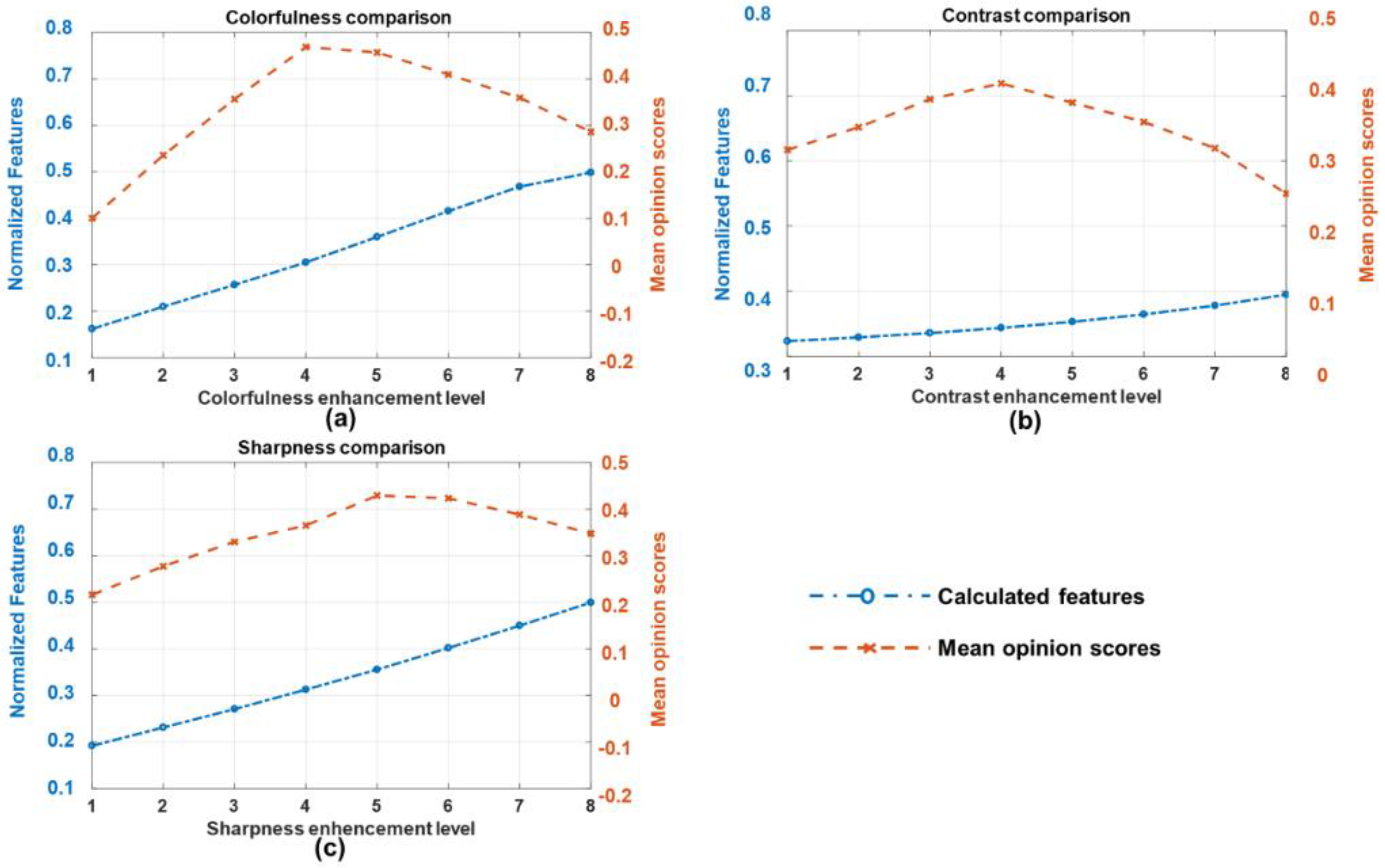
1.1. Correlation between the Evaluation Scores and the Adjustment Levels

The feature values for colorfulness, contrast, and sharpness used in the CQE method can effectively represent the levels of each adjustment. As a result, the calculated quality scores obtained by linearly combining these values may represent the overall levels of the image adjustments. However, the subjective evaluation scores for these adjusted images may be different from the quality scores calculated by CQE because HVS perceives images differently than the calculated features and quality scores used in CQE do. As such, we conducted experiments to investigate the correlation between the subjective and calculated scores and the level of image adjustments.

Eight levels of the colorfulness, contrast, and sharpness adjustments were applied to 24 images in the TID2013 database [35], which resulted in 576 adjusted images. The color saturation method [36], linear contrast adjustment [37], and unsharp masking method [3] were used for colorfulness, contrast, and sharpness adjustments, respectively. Eight observers participated in subjective evaluations for these adjusted images and rated the image qualities from 1 to 5 with 1 representing the worst quality and 5 the best. Lastly, we calculated mean opinion scores [38] from these subjective scores.

Figure 1 shows the mean scores of the subjective scores and the calculated feature values used in a previous assessment method, CQE [30], along with the levels of image adjustment. While the calculated feature values keep increasing as the level of adjustment increases, the subjective scores increase only until the level of adjustment of about four or five levels and then they decrease thereafter until the eighth adjustment level. Figure 1 shows that the calculated feature values and the subjective scores have different tendencies depending on the level of adjustment. Generally, the subjective scoring is considered the gold standard for image assessment methods because human perception is the ultimate image receiver. This suggests that excessive adjustment of an image can have adverse impact on the perception of HVS for the image. Therefore, in this study, we propose a new fully automatic assessment method that can consider the relationships between the adjustment levels and the visual preference of HVS. Our assessment algorithm utilizes the features of HDR images, which are better matched with HVS preferences than LDR images. The following Section 2.2 demonstrates that HDR images receive higher subjective evaluation scores than LDR images.

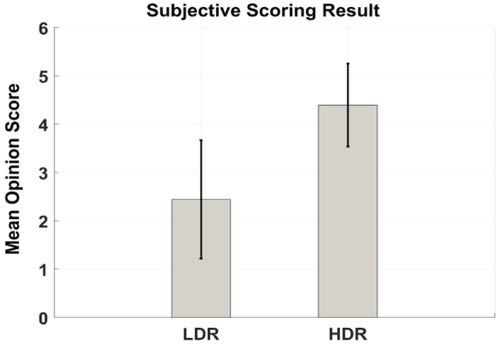
1.2. Visual Preference Comparison between LDR and HDR Images

To determine whether the visual preference for HDR images is greater than for LDR images, we subjectively evaluated the HDR and LDR images. A total of 190 LDR images and 27 tone-mapped HDR images from the EMPA-HDR database [39] were subjectively evaluated by 10 researchers who specialize in image processing for analysis, image adjustment, and artifact reduction in a dark room display and the same display. The random order images were individually evaluated on a scale of 1 (minimum score) to 5 (maximum score). The subjective scores evaluated by 10 observers of each images were averaged to yield mean opinion scores (MOSs) and the MOSs of all LDR and tone mapped HDR images were also averaged to yield total MOSs of LDR and tone mapped HDR, respectively. Figure 2 shows that the subjective scores for the HDR images are greater than those for the LDR images. While the mean score of the LDR images is 2.44, the mean score of the HDR images is 4.39. This indicates that the HDR images are visually preferred by HVS over the LDR images.

Our proposed assessment method, therefore, uses HDR-derived features extracted from HDR images that are closer to the HVS properties in order to improve our method’s correlation with subjective evaluations.

2. Materials and Methods

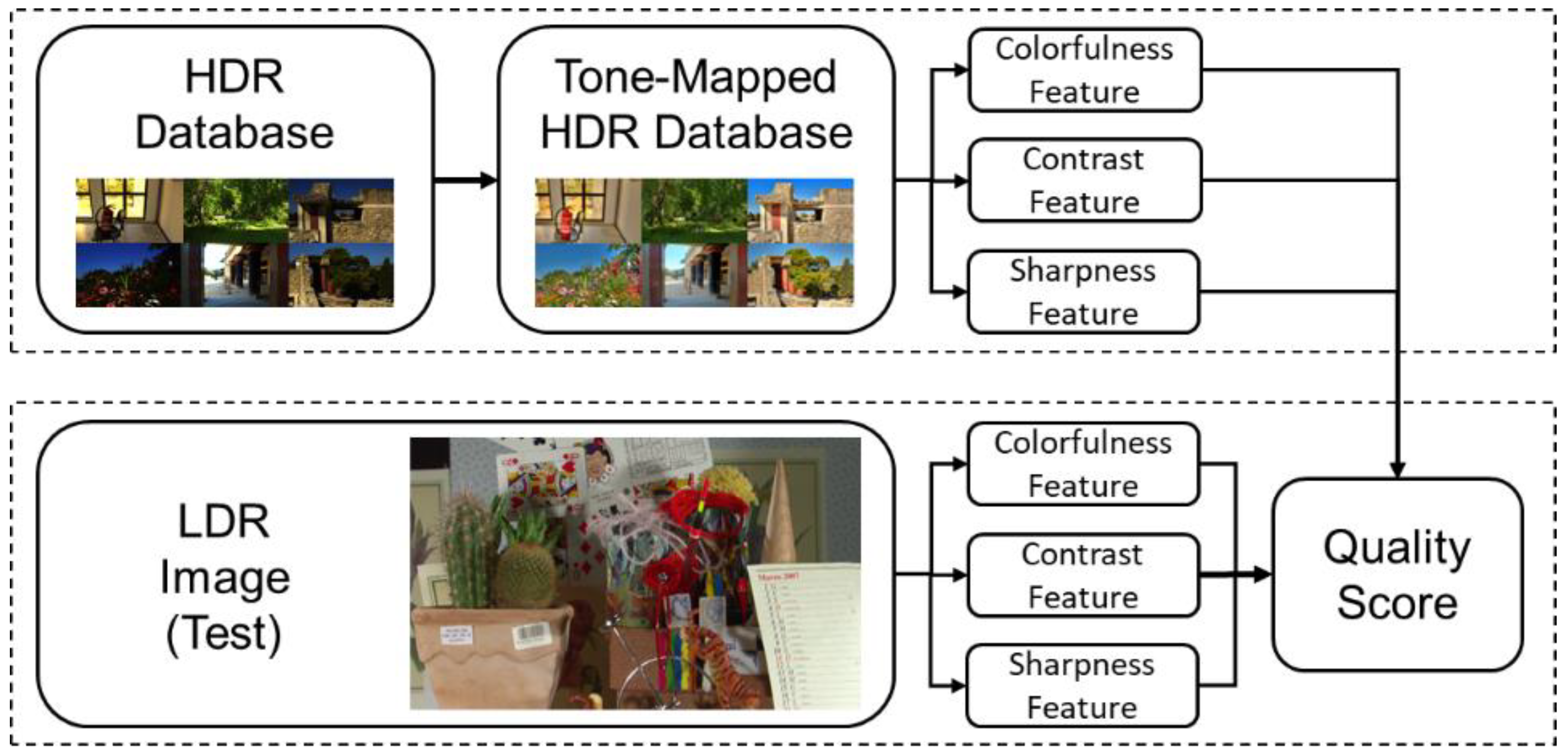
2.1. Proposed Assessment Method

Since the visual preference for HDR images is higher than for LDR images, a better quality score can be obtained by using the calculations based on the difference between the HDR-derived features and the test image features. The features used in our method are HDR-derived colorfulness, contrast, and sharpness features. In addition, each colorfulness, contrast, and sharpness feature in our method comprises global and local feature values. Since HVS evaluates images based on the hierarchical visual perception mechanism [40], our proposed method uses both global and local features to consider these HVS properties.

HDR images have different bit depth than LDR images and cannot be directly compared with them. Therefore, the HDR images are first tone-mapped [41] such that the scale of the original HDR images can be matched to those of the LDR test images. 500 HDR images were used to construct the standard HDR-derived features.

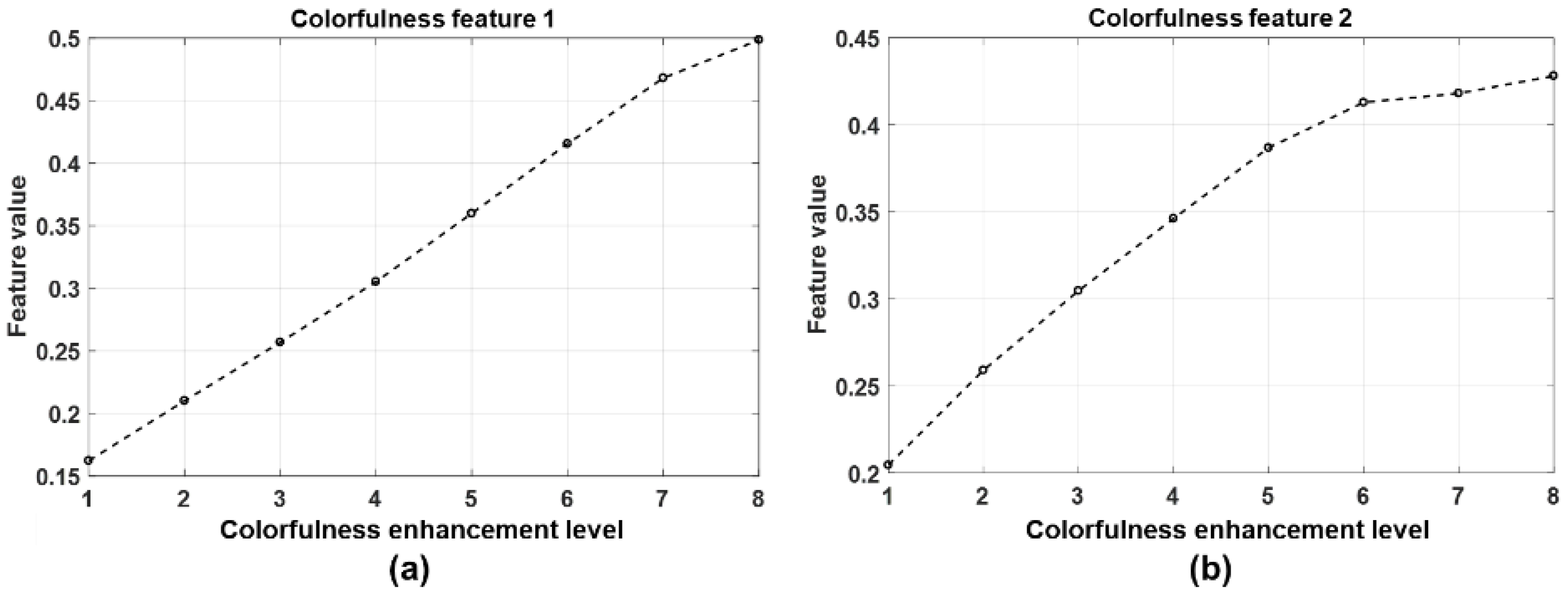
2.1.1. Colorfulness

Colorfulness is an aspect of the visual perception, according to which the color of an object is perceived to be more or less chromatic [30]. The colorfulness features can be obtained mainly from color channels a and b of the CIELab space and they are orthogonal to the lightness channel. Two different colorfulness features are used in our proposed method. The first colorfulness feature is calculated by using Equation (1) [30].

$$Co{l}_1=0.02\times \log \left(\frac{{\sigma }_a^2}{{\left|{\mu }_a\right|}^{0.2}}\right)\times \log \left(\frac{{\sigma }_b^2}{{\left|{\mu }_b\right|}^{0.2}}\right)$$

(1)

where ${\sigma }_a^2$ and ${\sigma }_b^2$ are the variance of a and b channels in CIELab and ${\mu }_a$ and ${\mu }_b$ are the mean values of the a and b domains, respectively. This feature value increases as the color adjustment level increases, which is shown in Figure 3a.

Unlike CQE, our proposed method applies a low-pass filter to the RGB space before converting it into the CIELab space. This is done so that the colorfulness features are not influenced by the components of the structural features. The low-pass filter is effective in minimizing the influence of the sharpness features of the images.

The second colorfulness feature in our assessment method is obtained by using Equation (2).

$$Co{l}_2=\frac{1}{NM}{\displaystyle \sum }_{i=1}^N{\displaystyle \sum }_{j=1}^M\sqrt{{\displaystyle \sum }_{k=-K}^K{\displaystyle \sum }_{l=-L}^L{w}_{k,l}{\left(R_{k,l}\left(i,j\right)-\mu \left(i,j\right)\right)}^2}$$

(2)

where $R=\sqrt{a^2+b^2}$ is the magnitude of the color components in the chromatic domain, $w_{k,l}$ is the 5 × 5 sized 2D circularly symmetric Gaussian weighting function, and N and M are the width and height of an image, respectively. This feature also increases as the color adjustment level increases, which is shown in Figure 3b.

The first feature in Equation (1) represents the global colorfulness obtained from the entire image while the second feature in Equation (2) represents the local colorfulness obtained from small image patches. Our proposed method uses these two colorfulness features to consider the global and local aspects of the HVS color perception [40]. These feature values are compared with the HDR colorfulness features that are established from HDR images by using the same Equations (1) and (2) in order to determine the final quality scores that correlate well with the subjective evaluations.

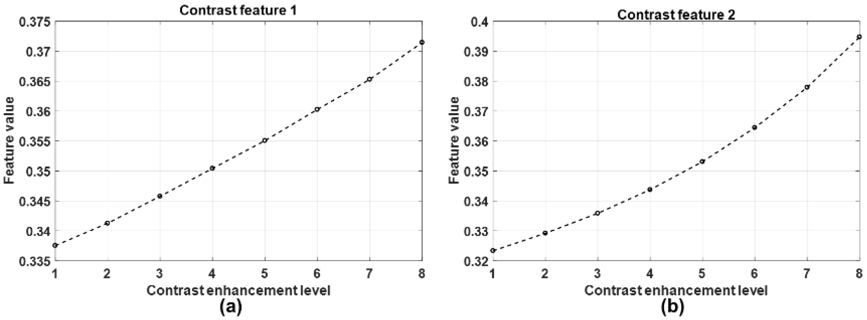
2.1.2. Contrast

Contrast represents the difference in luminance that makes an object distinguishable from other objects within the same field of view [30]. Similar to the colorfulness features, a low-pass filter is also used to minimize the influence of the sharpness component of an image in our study. The first feature is obtained by using Equation (3).

$$Co{n}_1=\frac{1}{k_1{k}_2}{\displaystyle \sum }_{l=1}^{k_1}{\displaystyle \sum }_{k=1}^{k_2}{\left(\log \left(\frac{L_{max,k,l}+L_{min,k,l}}{L_{max,k,l}-L_{min,k,l}}\right)\right)}^{-0.5}$$

(3)

where $L_{max}$ and $L_{min}$ are the maximum and minimum luminance values of a 5 × 5-sized image patches, respectively. This feature increases as the contrast adjustment level increases, which is shown in Figure 4a. The second contrast feature is obtained by using Equation (4).

$$Co{n}_2=\frac{1}{NM}{\displaystyle \sum }_{i=1}^N{\displaystyle \sum }_{j=1}^M\sqrt{{\displaystyle \sum }_{k=-K}^K{\displaystyle \sum }_{l=-L}^L{w}_{k,l}{\left(L_{k,l}\left(i,j\right)-\mu \left(i,j\right)\right)}^2}$$

(4)

where $w_{k,l}$ is a 15 × 15 2D circularly symmetric Gaussian weighting function. The second contrast feature also increases as the contrast adjustment level increases, which is shown in Figure 4b.

The first feature in Equation (3) represents the local contrast feature that is extracted from small-sized image patches. In contrast, the second feature in Equation (4) represents a semi-global contrast feature that is extracted from relatively large-sized image patches. As done with the colorfulness assessment, our proposed method uses two contrast features to consider the HVS properties. These feature values are also compared with the HDR contrast features for the final quality score calculations.

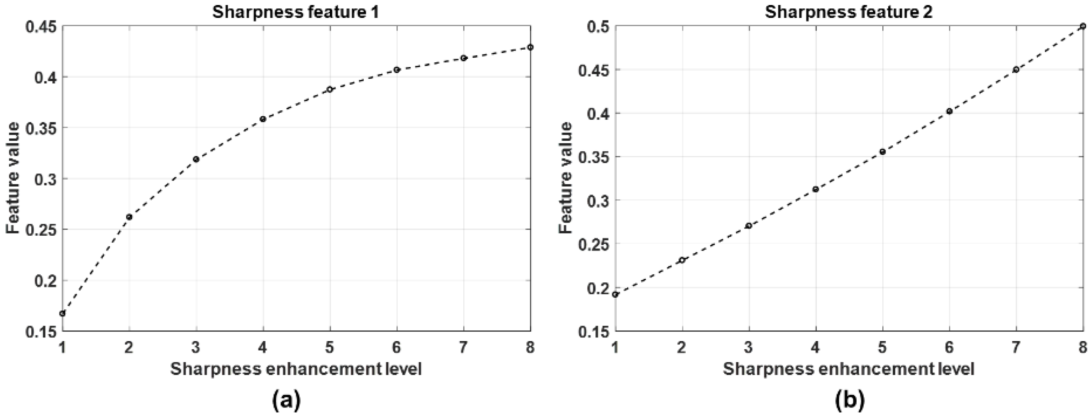
2.1.3. Sharpness

Sharpness represents the aspects of fine details and edge components of an image and it is distributed in the high-frequency band of a Fourier domain [30]. Sharpness features can be extracted from high-pass filtered images, which is outlined in Equations (5) and (6).

$$Sh{a}_1=\frac{1}{k_1{k}_2}{\displaystyle \sum }_{l=1}^{k_1}{\displaystyle \sum }_{k=1}^{k_2}\log \left(\frac{E_{max,k,l}}{E_{min,k,l}}\right)$$

(5)

The first sharpness feature in Equation (5) is calculated by using 5 × 5 sized image patches and $E_{max}$ and $E_{min}$ are the maximum and minimum luminance values of the high-pass filtered image patches, respectively. This feature increases as the sharpness adjustment level increases, which is shown in Figure 5a.

$$Sh{a}_2=\frac{1}{NM}{\displaystyle \sum }_{i=1}^N{\displaystyle \sum }_{j=1}^M\sqrt{{\displaystyle \sum }_{k=-K}^K{\displaystyle \sum }_{l=-L}^L{w}_{k,l}{\left(E_{k,l}\left(i,j\right)-\mu \left(i,j\right)\right)}^2}$$

(6)

The second sharpness feature is obtained by using Equation (6). The standard deviation of the high-pass filtered luminance values is used to calculate how widely distributed the high-frequency components were in the images. $w_{k,l}$ is a relatively large-sized 15 × 15 2D circularly symmetric Gaussian weighting function. This feature increases as the sharpness adjustment level increases, which is shown in Figure 5b. Similar to the assessments of the colorfulness and contrast, our proposed method uses both local (Equation (5)) and global (Equation (6)) sharpness features to consider the HVS properties. These feature values are also compared with the HDR sharpness features for the final quality score calculations.

2.1.4. HDR-Derived Features

A direct assessment using the previously mentioned features obtained from Equations (1)–(6) may lead to erroneous evaluation results that do not correlate well with the subjective evaluations, as previously demonstrated in Figure 1. To overcome this problem, our proposed assessment method uses HDR-derived features as standards when evaluating the features of a test image. The HDR-derived features are extracted by using the same equations (Equations (1)–(6)) applied to many HDR images. Since the HDR images are visually preferred by HVS as shown in Figure 2, HDR-derived features can be used as references, according to which the features of test images are evaluated to determine the final quality scores. Our study demonstrates that this method correlates well with the subjective evaluations.

2.1.5. Assessment Metric Scheme

Figure 6 shows a diagram of our proposed method for determining the quality score of a test image. Six features are extracted from a test image and then compared with the standard HDR-derived features to calculate the quality score of a test image.

First, the differences between each feature are calculated by using the following equation.

$$\Delta X=\left|X_{HDR}-X_{TEST}\right|$$

(7)

where $X_{HDR}$ is a standard HDR-derived single feature vector and the $X_{TEST}$ is a single feature vector of the test image. Many colorfulness, contrast, and sharpness features from HDR images is obtained and averaged to make a single feature vector. Lastly, the single feature vector is used to calculate the quality score based on a weighted combination of the feature differences. In addition, multiple feature vectors from a test image are also averaged to make a single feature vector since multiple feature vectors are obtained from multiple local patches of a single test image. The final quality score, Q, is obtained from a weighted combination of the following feature differences.

$$Q=\overrightarrow{C}\overrightarrow{D}=\left[C_1 C_2 C_3 C_4 C_5 C_6\right]\times {\left[\Delta Co{l}_1 \Delta Co{l}_2 \Delta Co{n}_1 \Delta Co{n}_2 \Delta Sh{a}_1 \Delta Sh{a}_2 \right]}^T$$

(8)

where $\overrightarrow{C}$ is a set of weighting coefficients for each feature. $\overrightarrow{C}$ was determined as [7, 9, 6.1, 8.5, 6.7, 0.54, 1] through the training with 576 training image sets.

2.2. Experimental Setup

The total 576 training images were subjectively evaluated by 10 researchers who specialize in image processing for analysis, image adjustment, and artifact reduction in the dark room display and in the same display. The random order images were individually evaluated on a scale of 1 (minimum score) to 5 (maximum score).

A total of 114 adjusted images were assessed by our proposed method as well as by two conventional methods, which were NIQE and CQE. The subjective evaluation was also performed as the ground truth quality scores. Three intact images (traffic, cactus, and basketball) were selected from the LIVE video database [42] and processed with different combinations of three levels of colorfulness adjustment, three levels of contrast adjustment, and four levels of sharpness adjustment, which resulted in 108 adjusted images using MATLAB (R2017a, The Mathworks, Natick, MA, USA) software automatically. The examples of these test image sets are shown in Figure 7. The other six images included the original three images plus enhanced ones by an HDR-toning toolbox in Photoshop CS6. These 114 test images were not used in the training process.

3. Evaluation Results

To evaluate the performance of our proposed method, we obtained correlations between the quality scores of our proposed method and the subjective scores (visual preferences of HVS). Ten observers participated in the subjective evaluation. For the purpose of comparison with other methods, correlations between the scores of the conventional methods (NIQE and CQE) and the subjective scores were also obtained. Spearman’s rank ordered a correlation coefficient (SROCC) and Pearson’s linear correlation coefficient (PLCC), which were used to compare the performances. We used the Spearman and Pearson coefficients methods for performance evaluation because these methods have been widely used for correlation metrics between image quality assessment and subjective scores [21,22,23,24,25].

The results of the correlations with the subjective scores are shown in

Table 1. Performance comparison between the conventional methods (NIQE, CQE) and the proposed method. Two difference correlation metrics called SROCC and PLCC were calculated between the scores measured by the automatic methods and by the subjective evaluation.

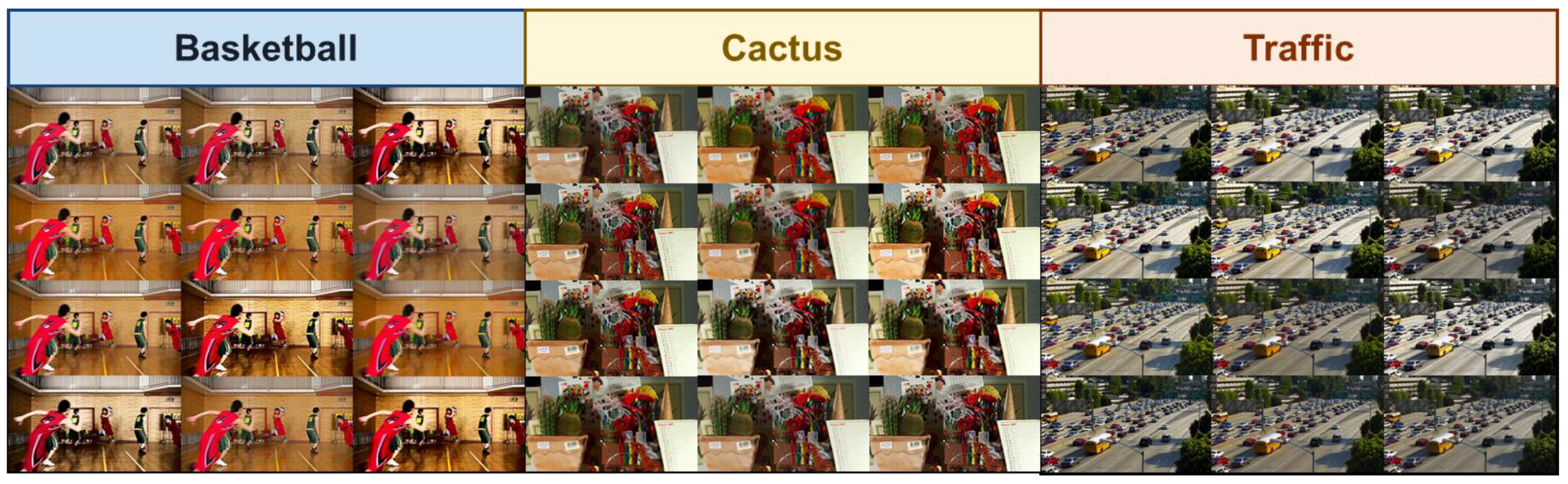
		Basketball	Cactus	Traffic	Average
NIQE	SROCC	0.6465	0.3233	0.1650	0.3283
	PLCC	0.7144	0.3221	0.2373	0.4246
CQE	SROCC	0.6207	0.4241	0.5292	0.5247
	PLCC	0.6225	0.4236	0.5205	0.5222
Proposed Method	SROCC	0.8042	0.9121	0.9669	0.8944
	PLCC	0.7626	0.9284	0.9538	0.8816

. In all the cases, our proposed method achieved higher correlations with the subjective scores than those of the NIQE and CQE. These results demonstrate that our proposed method is more suitable for evaluating the colorfulness-adjusted, contrast-adjusted, and sharpness-adjusted images than the other two conventional methods. This is because the conventional methods were mainly developed for evaluating images distorted by compression or noise corruption (NIQE) and did not consider HVS properties (CQE).

4. Discussion and Conclusions

We proposed a fully automatic no-reference quality assessment method for the enhanced images whose colorfulness, contrast, and sharpness were adjusted. HDR-derived features were obtained from HDR images with different scenes. Therefore, the proposed method without using the reference image with the same scene can be a ‘no-reference’ method.

The proposed method does not require a reference image. It automatically calculates quantitative scores, visual preference, and quality assessment with respect to the level of colorfulness, contrast, and sharpness adjustment. This method considers colorfulness components. Additionally, this method uses HDR-derived features, which have more human visual preference than LDR images. By evaluating the LDR based on the HDR, this method can extract how different the quality of the test images differs from the HDR with a high visual preference and it offers visual preference scores, quantitatively. It shows that the proposed method yielded better performance than other methods.

We investigated the performance of the proposed method depending on the size of image patches in global and local settings and measured the corresponding performance, according to the correlation values with subjective scores. In most cases involving our test image dataset, the highest correlation results were achieved with the sizes of image patches used in our experiments.

Our proposed method currently used linear weighted coefficients trained by 576 HDR images. However, other machine learning metrics such as the support vector machine can be used in the training process. Because SVM-based quality evaluation methods have already been used in the detection on artifacts caused by compression [21,22,23,24,25], it is possible to use the SVM method for our proposed method. In addition, if there are additional features including the six features, neural network methods can be used for the evaluation of adjusted images.

We made an effort to overcome the limitations of conventional methods such as NIQE and CQE methods. NIQE performs well in evaluating the distorted images due to compression, blurring, or noise corruption, but it is not focused on evaluating adjusted images. CQE can evaluate several adjustment effects such as colorfulness and contrast adjustments but does not incorporate HVS properties in its assessment process, which results in a mismatch with the subjective evaluations. These limitations were effectively overcome in our proposed method, which incorporated HVS-favorable HDR-derived features as standards in its evaluation process. HDR images have higher visual preferences for HVS than LDR images and, therefore, the features derived from HDR images are more closely related to the perception properties of HVS than those of LDR images. In addition to the incorporation of the HDR-derived features, both global and local features are extracted and combined to produce the final quality scores for an image assessment, which also considers the hierarchical visual perception mechanism of HVS. Consequently, we found through our experimentation that our new assessment method correlated well with subjective evaluations and outperformed two conventional assessment methods.

References

- Danielyan, A.; Katkovnik, V.; Egiazarian, K. BM3D Frames and Variational Image Deblurring. IEEE Trans. Image Process. 2012, 21, 1715–1728. [Google Scholar] [CrossRef] [PubMed] [Green Version]
- Portilla, J.; Strela, V.; Wainwright, M.; Simoncelli, E. Image denoising using scale mixtures of gaussians in the wavelet domain. IEEE Trans. Image Process. 2003, 12, 1338–1351. [Google Scholar] [CrossRef] [PubMed] [Green Version]
- Polesel, A.; Ramponi, G.; Mathews, V. Image enhancement via adaptive unsharp masking. IEEE Trans. Image Process. 2000, 9, 505–510. [Google Scholar] [CrossRef] [PubMed] [Green Version]
- Yu, H.; Zhao, L.; Wang, H. Image Denoising Using Trivariate Shrinkage Filter in the Wavelet Domain and Joint Bilateral Filter in the Spatial Domain. IEEE Trans. Image Process. 2009, 18, 2364–2369. [Google Scholar] [PubMed]
- Kazubek, M. Wavelet domain image denoising by thresholding and Wiener filtering. IEEE Signal Process. Lett. 2003, 10, 324–326. [Google Scholar] [CrossRef]
- Stark, J. Adaptive image contrast enhancement using generalizations of histogram equalization. IEEE Trans. Image Process. 2000, 9, 889–896. [Google Scholar] [CrossRef] [PubMed] [Green Version]
- Park, S.; Park, M.; Kang, M. Super-resolution image reconstruction: A technical overview. IEEE Signal Process. Mag. 2003, 20, 21–36. [Google Scholar] [CrossRef]
- Yang, J.; Wright, J.; Huang, T.S.; Ma, Y. Image super-resolution via sparse representation. IEEE Trans. Image Process. 2010, 19, 2861–2873. [Google Scholar] [CrossRef] [PubMed]
- Zhou, D.; Wang, R.; Lu, J.; Zhang, Q. Depth Image Super Resolution Based on Edge-Guided Method. Appl. Sci. 2018, 8, 298. [Google Scholar] [CrossRef]
- Lai, J.; Liaw, Y.; Lo, W. Artifact reduction of JPEG coded images using mean-removed classified vector quantization. Signal Process. 2002, 82, 1375–1388. [Google Scholar] [CrossRef]
- Lee, R.; Kim, D.; Kim, T. Regression-based prediction for blocking artifact reduction in JPEG-compressed images. IEEE Trans. Image Process. 2005, 14, 36–48. [Google Scholar] [PubMed]
- Lucchese, L.; Mitra, S.; Mukherjee, J. A new algorithm based on saturation and desaturation in the xy chromaticity diagram for enhancement and re-rendition of color images. In Proceedings of the International Conference on Image Processing, Thessaloniki, Greece, 7–10 October 2001; Volume 2, pp. 1077–1080. [Google Scholar]
- Naik, S.; Murthy, C. Hue-preserving color image enhancement without gamut problem. IEEE Trans. Image Process. 2003, 12, 1591–1598. [Google Scholar] [CrossRef] [PubMed] [Green Version]
- Agaian, S.; Silver, B.; Panetta, K. Transform Coefficient Histogram-Based Image Enhancement Algorithms Using Contrast Entropy. IEEE Trans. Image Process. 2007, 16, 741–758. [Google Scholar] [CrossRef] [PubMed]
- Panetta, K.; Wharton, E.; Agaian, S. Human Visual System-Based Image Enhancement and Logarithmic Contrast Measure. IEEE Trans. Syst. Man Cybern. Syst. 2008, 38, 174–188. [Google Scholar] [CrossRef] [PubMed] [Green Version]
- Zhang, B.; Allebach, J. Adaptive Bilateral Filter for Sharpness Enhancement and Noise Removal. IEEE Trans. Image Process. 2008, 17, 664–678. [Google Scholar] [CrossRef] [PubMed]
- Panetta, K.; Agaian, S.; Zhou, Y.; Wharton, E. Parameterized Logarithmic Framework for Image Enhancement. IEEE Trans. Syst. Man Cybern. Syst. 2011, 41, 460–473. [Google Scholar] [CrossRef] [PubMed]
- Gu, K.; Zhai, G.; Yang, X.; Zhang, W.; Chen, C. Automatic Contrast Enhancement Technology with Saliency Preservation. IEEE Trans. Circuits Syst. Video Technol. 2015, 25, 1480–1494. [Google Scholar]
- Ferzli, R.; Karam, L. A No-Reference Objective Image Sharpness Metric Based on the Notion of Just Noticeable Blur (JNB). IEEE Trans. Image Process. 2009, 18, 717–728. [Google Scholar] [CrossRef] [PubMed] [Green Version]
- Liu, A.; Lin, W.; Paul, M.; Deng, C.; Zhang, F. Just Noticeable Difference for Images with Decomposition Model for Separating Edge and Textured Regions. IEEE Trans. Circuits Syst. Video Technol. 2010, 20, 1648–1652. [Google Scholar] [CrossRef]
- Moorthy, A.; Bovik, A. Blind Image Quality Assessment: From Natural Scene Statistics to Perceptual Quality. IEEE Trans. Image Process. 2011, 20, 3350–3364. [Google Scholar] [CrossRef] [PubMed]
- Saad, M.; Bovik, A.; Charrier, C. Blind Image Quality Assessment: A Natural Scene Statistics Approach in the DCT Domain. IEEE Trans. Image Process. 2012, 21, 3339–3352. [Google Scholar] [CrossRef] [PubMed]
- Mittal, A.; Moorthy, A.; Bovik, A. No-Reference Image Quality Assessment in the Spatial Domain. IEEE Trans. Image Process. 2012, 21, 4695–4708. [Google Scholar] [CrossRef] [PubMed] [Green Version]
- Mittal, A.; Soundararajan, R.; Bovik, A. Making a “Completely Blind” Image Quality Analyzer. IEEE Signal Process. Lett. 2013, 20, 209–212. [Google Scholar] [CrossRef]
- Zhang, Z.; Wang, H.; Liu, S.; Durrani, T.S. Deep Activation Pooling for Blind Image Quality Assessment. Appl. Sci. 2018, 8, 478. [Google Scholar] [CrossRef]
- Gu, K.; Zhai, G.; Lin, W.; Liu, M. The Analysis of Image Contrast: From Quality Assessment to Automatic Enhancement. IEEE Trans. Cybern. 2016, 46, 284–297. [Google Scholar] [CrossRef] [PubMed]
- Kim, H.; Ahn, S.; Kim, W.; Lee, S. Visual Preference Assessment on Ultra-High-Definition Images. IEEE Trans. Broadcast. 2016, 62, 757–769. [Google Scholar] [CrossRef]
- Feichtenhofer, C.; Fassold, H.; Schallauer, P. A Perceptual Image Sharpness Metric Based on Local Edge Gradient Analysis. IEEE Signal Process. Lett. 2013, 20, 379–382. [Google Scholar] [CrossRef]
- Gu, K.; Zhai, G.; Lin, W.; Yang, X.; Zhang, W. No-Reference Image Sharpness Assessment in Autoregressive Parameter Space. IEEE Trans. Image Process. 2015, 24, 3218–3231. [Google Scholar] [PubMed]
- Panetta, K.; Gao, C.; Agaian, S. No reference color image contrast and quality measures. IEEE Trans. Consum. Electron. 2013, 59, 643–651. [Google Scholar] [CrossRef]
- Panetta, K.; Bao, L.; Agaian, S. A human visual “no-reference” image quality measure. IEEE Instrum. Meas. Mag. 2016, 19, 34–38. [Google Scholar] [CrossRef]
- Reinhard, E. High Dynamic Range Imaging; Elsevier Morgan Kaufmann: Amsterdam, The Netherlands, 2010. [Google Scholar]
- Ofili, C.; Glozman, S.; Yadid-Pecht, O. Hardware Implementation of an Automatic Rendering Tone Mapping Algorithm for a Wide Dynamic Range Display. J. Low Power Electron. Appl. 2013, 3, 337–367. [Google Scholar] [CrossRef] [Green Version]
- Cauwerts, C.; Piderit, M.B. Application of High-Dynamic Range Imaging Techniques in Architecture: A Step toward High-Quality Daylit Interiors? J. Imaging 2018, 4, 19. [Google Scholar] [CrossRef]
- Ponomarenko, N.; Jin, L.; Ieremeiev, O.; Lukin, V.; Egiazarian, K.; Astola, J.; Vozel, B.; Chehdi, K.; Carli, M.; Battisti, F.; et al. Image database TID2013: Peculiarities, results and perspectives. Signal Process. Image Commun. 2015, 30, 57–77. [Google Scholar] [CrossRef] [Green Version]
- Lübbe, E. Colours in the Mind-Colour Systems in Reality; Books on Demand: Norderstedt, Germany, 2010. [Google Scholar]
- Al-amri, S.; Kalyankar, N.; Khamitkar, S. Linear and non-linear contrast enhancement image. Int. J. Comput. Sci. Netw. Secur. 2010, 10, 139–143. [Google Scholar]
- Streijl, R.; Winkler, S.; Hands, D. Mean opinion score (MOS) revisited: Methods and applications, limitations and alternatives. Multimed. Syst. 2014, 22, 213–227. [Google Scholar] [CrossRef]
- EMPA Media Technology. Available online: http://www.empamedia.ethz.ch/hdrdatabase/index.php (accessed on 25 January 2017).
- Wang, Z.; Simoncelli, E.; Bovik, A. Multi-scale structural similarity for image quality assessment. In Proceedings of the Thirty-Seventh Asilomar Conference on Signals, Systems & Computers, Pacific Grove, CA, USA, 9–12 November 2003; Volume 2, pp. 1398–1402. [Google Scholar]
- Ashikhmin, M.; Goyal, J. A reality check for tone-mapping operators. ACM Trans. Appl. Percept. 2006, 3, 399–411. [Google Scholar] [CrossRef]
- Seshadrinathan, K.; Soundararajan, R.; Bovik, A.; Cormack, L. Study of Subjective and Objective Quality Assessment of Video. IEEE Trans. Image Process. 2010, 19, 1427–1441. [Google Scholar] [CrossRef] [PubMed] [Green Version]