Multiple-Penalty-Weighted Regularization Inversion for Dynamic Light Scattering

School of Electrical and Electronic Engineering, Shandong University of Technology, Zibo 255049, China
*
Author to whom correspondence should be addressed.
Appl. Sci. 2018, 8(9), 1674; https://doi.org/10.3390/app8091674
Submission received: 25 July 2018
/
Revised: 7 September 2018
/
Accepted: 13 September 2018
/
Published: 16 September 2018
(This article belongs to the Section Optics and Lasers)
Abstract
:By using different weights to deal with the autocorrelation function data of every delay time period, the information utilization of dynamic light scattering can be obviously enhanced in the information-weighted constrained regularization inversion, but the denoising ability and the peak resolution under noise conditions for information-weighted inversion algorithm are still insufficient. On the basis of information weighting, we added a penalty term with the function of flatness constraints to the objective function of the regularization inversion, and performed the inversion of multiangle dynamic light scattering data, including the simulated data of bimodal distribution particles (466/915 nm, 316/470 nm) and trimodal distribution particles (324/601/871 nm), and the measured data of bimodal distribution particles (306/974 nm, 300/502 nm). The results of the inversion show that multiple-penalty-weighted regularization inversion can not only improve the utilization of the particle size information, but also effectively eliminate the false peaks and burrs in the inversed particle size distributions, and further improve the resolution of peaks in the noise conditions, and then improve the weighting effects of the information-weighted inversion.
1. Introduction
Dynamic light scattering (DLS), as a noncontact and noninterference with the original state of the measured system, has become a common method for submicron and nanoparticle measurement [1,2,3]. This DLS technique uses the photon correlation spectroscopy (PCS) [4,5] and obtains information of particle size distribution (PSD) by recovering the autocorrelation function (ACF) of the light intensity scattered by Brownian particles. However, the inversion of ACF data is an inherently difficult problem in DLS measurements, as a Fredholm integral equation of the first kind needs to be solved. As an ill-conditioned equation, the existence, uniqueness, and stability of the solution are uncertain. A variety of the inversion methods have been proposed, including the cumulants method [6], the Laplace transform method [7], the non-negative least-squares method (NNLS) [8], the constrained regularization method (CONTIN) [9,10], singular value decomposition method [11], and the regularization method [12,13,14]. In addition, some improved techniques have been proposed containing a modified cumulants method [15,16,17], a regularized NNLS [18], a modified regularization algorithm [19], a modified truncated singular value decomposition [20], and many intelligent optimization-based algorithms [21,22,23,24,25] used in DLS inversion. Each of these methods has its own characteristics and limitations, and the inversion of the bimodal or multimodal distribution particles has always been a difficult problem.
In 1987, Cummins and Staples [26] used two-angle DLS and showed the advantages of multiangle DLS over single-angle DLS for the bimodal PSD inversion. In 1995, Bryant and Thomas [27] further improved the accuracy of PSD recovery by combining MDLS data with high-quality static light scattering (SLS) data and analyzing the data simultaneously. In order to make better use of the advantages of multiangle measurement, Vega et al. [28] proposed a recursive least-squares method to estimate the weighting coefficients using the complete ACF measurement and a regularization parameter in 2003. In 2012, Liu et al. [29] developed an iterative recursion method for obtaining the required intensity weighting and proved the relationship between the inversion accuracy and the number of scattering angles used in multiangle DLS.
In 2016, Zhu et al. introduced the idea of signal weighting into DLS technique for PSD inversion, in which the light intensity ACF was used to weight the residual in the regularization inversion [30], and the noise effect of the long delay period in ACF was attenuated. In 2018, Xu et al. proposed an information-weighted method and a character-weighted method for DLS inversion [31,32], in which the different weights were used to deal with the data of every delay time period in the ACF. By means of the weighting, the utilization of the ACF data is increased in the information-intensive segments and decreased in the noise-intensive segments, which means that a higher availability of information in ACF has been achieved and the noise effect still exists in the information-intensive segments. However, for the inversion of the bimodal or multimodal distribution particles, the noise distributed in ACF, no matter in which delay segment, has an impact on peak recognition. In this paper, by adding a penalty term with a flatness constraint function in the objective function, the multiple-penalty-weighted regularization is used to inverse the ACF data. By eliminating the false peaks and burrs in the inversion, the peak recognition ability is improved and the PSDs can be better retrieved in the noise conditions.
2. Dynamic Light Scattering and Multiple-Penalty-Weighted Regularization
In DLS measurement, the scattering light intensity ACF at the scattering angle θ can be described as follows:
where is the discrete ACF of the scattered light intensity, iθ(τk) the scattered light intensity at the delay time , τj the discrete delay time, and M the total number of samples acquired by the correlator. The light intensity ACF is related to the normalized electric field ACF, , by the Siegert relationship [33]
where B is the measured baseline of , β (≤1) is the instrumental coherence constant, and j (1 ≤ j ≤ M) is the channel number of the correlator.
The normalized electric field ACF has the form [8]
where d, kB, T, λ0, nm, η, and f(di) are the diameter of spherical particle, the Boltzmann constant, the absolute temperature of the medium, the wavelength of the incident light, the refractive index of the nonabsorbing suspending medium, the viscosity of the dispersing medium, and the discrete PSD, respectively. Equation (3) can be simplified as
where is a vector with elements , f a vector with elements f(di), and Aθ a kernel matrix corresponding to the measured ACF at the scattering angle θ. The elements of Aθ are given by
Tikhonov regularization method for DLS inversion needs to minimize the objective function
where α is the regularization parameter, L the regularization matrix, f the estimated PSD, ‖·‖the Euclidean norm, and the penalty functional factor. Generally, the regularization parameter α is determined by L-curve criterion [34,35] to control the accuracy and stability of the solution, and the identity matrix is chosen as the regularization matrix. The weighted regularization inversion form [31,32] of Equation (6) is
where is the weighted matrix, and
where AW is the kernel matrix of Equation (8), AW = [; ; …; ], and is a vector set containing the weighted electric field ACF data at scattering angles θ1, θ2, …, θm. is the electric field ACF data at scattering angle θr, the kernel matrix corresponding to , Wθr the weighted matrix corresponding to , kr the constant related to the scattering angle θr, and r an integer from 1 to m.
where Pr is the weight-adjusting parameter and is the ACF data from the actual measurement. Adding a new penalty item in the objective function of the weighted regularization, then
where is the newly increased regularization parameter. L, the regular matrix in the first penalty term, is a zero-order matrix (identity matrix), and L1, the regular matrix in the second penalty term, is a first-order matrix [36]. Regularization parameters can be selected by fixed-point iteration method or model function method [37]. In this work, fixed-point iteration method is used and, by optimizing minimum distance function (MDF) [38], the iterative model for obtaining the second regularization parameters is derived as
where and are the squares of the smallest and the largest singular values of the AW matrix, respectively.
The steps of selecting regularization parameters are as follows: Firstly, the regularization parameter α is selected through the L-curve criterion, and and are calculated. By assuming the initial regularization parameter β(0) with , is calculated. Secondly, β(0), βa, βb, and are substituted into the Equation (12), and the second parameter and its corresponding solution are obtained. Thirdly, it is determined whether the iteration stop condition, , is satisfied. Repeat the last two steps in turn if the stop condition is not met, until the condition is satisfied. , which satisfies the iteration stop condition, is the optimal regularization parameter.
3. Numerical Simulation and Analysis
In the simulations, both bimodal particles and trimodal particles were involved by using Johnson’s SB function [39]
where t = (d − dmin)/(dmax − dmin) is the normalized particle size. dmax and dmin are the maximum and the minimum particle size, respectively. μ and σ are distribution parameters. The intensity ACF data can be obtained by Equation (1). Two performance indices were introduced for examining the inversion performance:
where is the simulated “true” PSD, the retrieved PSD, Ptrue the peak position value of the simulated “true” PSD, and Pmeas the peak position value of the retrieved PSD. The smaller the V1 and V2 values, the better the performance of the inversion. The parameters of simulated PSD are shown in Table 1. d1, d2, and d3 are the particle size corresponding to the peak position value of PSD. Simulations were conducted with the conditions: kB = 1.3807 × 10⁻²³ J/K, T = 298.15 K, η = 0.89 cP, nm = 1.3316, λ0 = 632.8 nm, θr = 30°, 50°, 70°, 90°, 110°, 130°. AS, BS, and CS represent far bimodal 466/915 nm, near bimodal 316/470 nm, and trimodal 324/601/871 nm simulated PSD, respectively. The size distribution ranges of AS, BS, and CS are [2.01 nm, 1200.01 nm], [2.01 nm, 800.01 nm], and [2.01 nm, 1200.01 nm], respectively, and the discrete points of all simulated distributions are 160. The inversion results are shown in Figure 1, Figure 2 and Figure 3, and the corresponding performance indices are shown in Table 2, Table 3 and Table 4. In the Figures, the subtitles (a), (b), (c), and (d) are the inversion results with noise levels of 0, 10−4, 10−2, and 0.8, respectively. ‘True PSD’, ‘WR’ and ‘WMR’ represent the true PSD, the inversed PSD by weighted regularization, and the inversed PSD by multiple-penalty-weighted regularization.
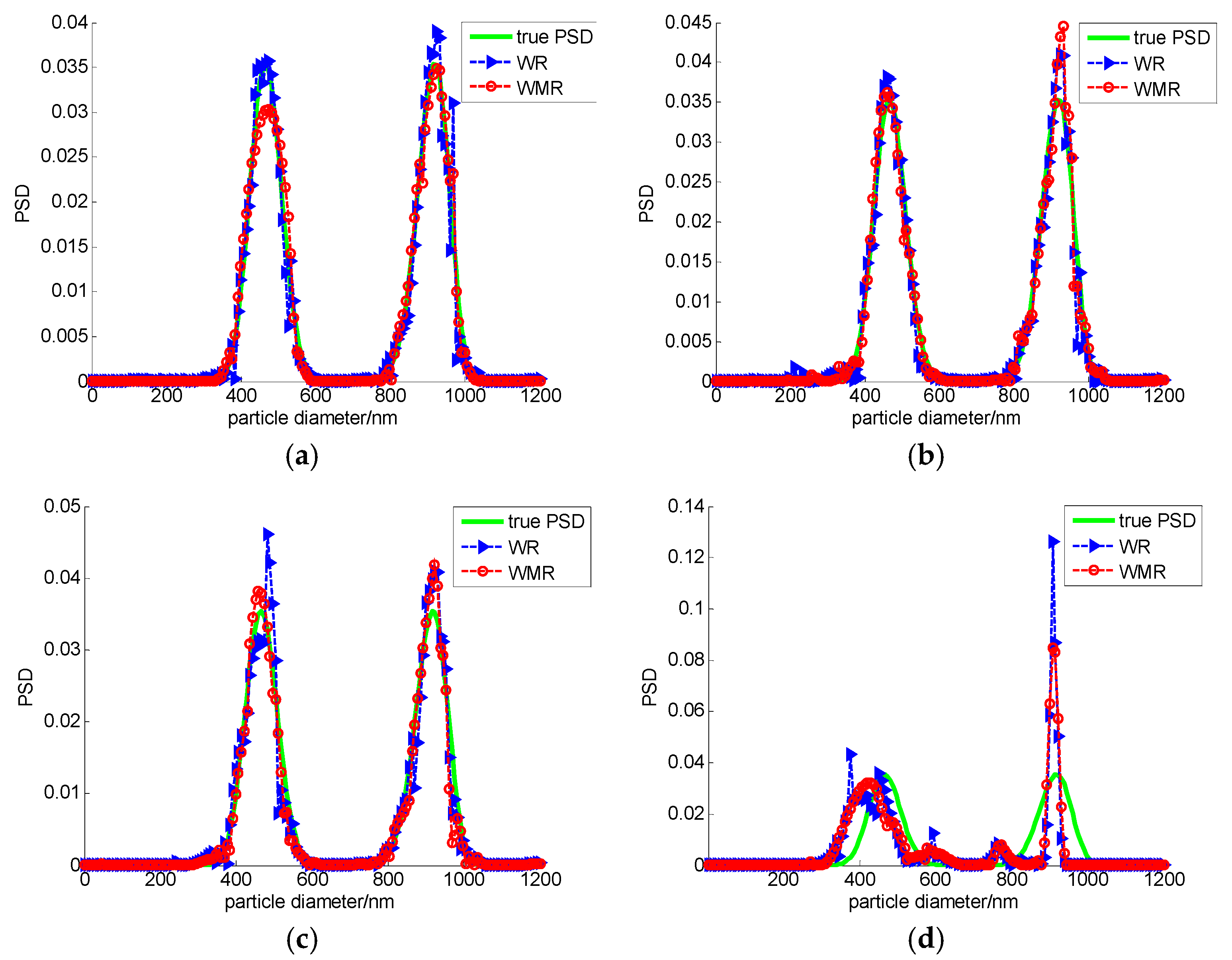
The inversion results, with the single-penalty and the multiple-penalty-weighted regularization from 466/915 nm bimodal simulated DLS data, are shown in Figure 1. It is obvious that, with the increase of the added noise, there are obvious burrs in the PSDs inversed by weighted regularization function. When the noise level reaches 0.08, an obvious false peak is found in the PSDs inversed by single-penalty-weighted regularization. After adding another penalty to the objective function, some false peaks and burrs are eliminated, and a bimodal PSD, which is relatively close to the true PSD, is still obtained. From the corresponding performance indices (Table 2), it can be seen that the fitting errors and peak position errors are reduced obviously by using the multiple-penalty-weighted regularization method.
The retrieved PSDs, with the single-penalty and the multiple-penalty-weighted regularization from 316/470 nm bimodal simulated DLS data, are shown in Figure 2 and the corresponding performance indices are shown in Table 3. From Figure 2, it can be seen that in addition to the obvious burrs and false peaks in the results inversed by single-penalty-weighted regularization, the jump also occurs in the size distribution as the noises increase, and this situation is improved by adding a penalty term in the weighted inversion. When the noise level reaches 0.08, large peak deviations occur in the inversed PSDs for both methods, while the results obtained by the multiple-penalty-weighted regularization are relatively better than those obtained by the single-penalty one in terms of the peak values and burr occurrence. Table 3 indicates that all the fitting errors and the peak position errors in the PSDs obtained by the multiple-penalty-weighted regularization are obviously less than that by the single-penalty-weighted regularization.
Figure 3 shows the inversion results of the single-penalty and the multiple-penalty-weighted regularization for 324/601/871 nm trimodal simulated DLS data, and Table 4 gives the corresponding performance indices. From Figure 3 and Table 4, we can see that the multiple-penalty-weighted regularization effectively eliminates the burr and spurious peaks which appeared in the PSDs inversed by single-penalty-weighted regularization. Both the peak errors and peak position errors of the former are obviously smaller than that of the latter.
4. Experimental Data Inversion
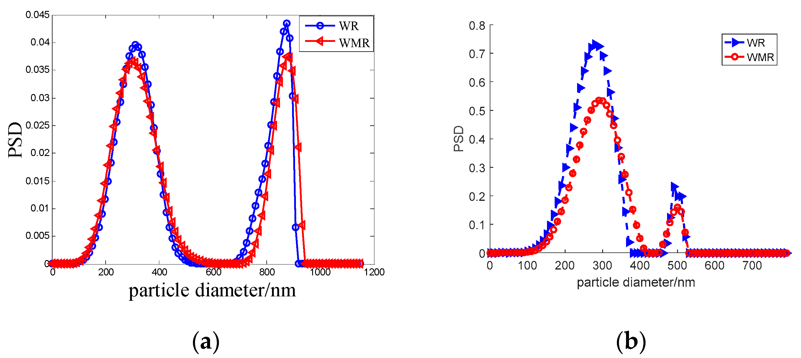
The experimental data corresponding to two bimodal samples (AE, BE) were used to evaluate multiple-penalty-weighted regularization inversion. Sample AE was obtained by mixing 306 nm ± 8 nm and 974 nm ± 10 nm standard polystyrene latex spheres (Polyscience Inc., Warrington, PA, USA), and sample BE by mixing 300 nm ± 3 nm and 502 nm ± 4 nm standard polystyrene latex spheres (Duke Scientific Corporation, Palo Alto, CA, USA). For both bimodal samples, the regulated sample temperature T = 298.15 K, and the dispersion medium refractive index nm = 1.33. The measured DLS data was obtained at the scattering angle θ = 30°, 50°, 70°, 90°, 110°, 130° for sample AE, and θ = 30°, 50°, 70°, 90°, 110°, 120° for sample BE. Figure 4 shows the recovered PSDs, and the value of the performance indices are shown in Table 5.
As can be seen from Figure 4, the weighted regularization, with single or multiple penalty, can all retrieve a bimodal PSD, but their inversion errors are obviously different. The recovered peak positions obtained by the multiple-penalty-weighted regularization are closer to the true positions than those by the single-penalty-weighted regularization. The performance indices in Table 5 show that the relative errors given by the multiple-penalty-weighted regularization are obviously reduced compared with those by the single-penalty-weighted regularization. For the 360 nm and 974 nm peaks, the relative errors are reduced from 0.0228 and 0.1027 to 0.0196 and 0.0903, respectively, and for the 360 nm and 974 nm peaks, from 0.0667 and 0.0239 to 0.0333 and 0.0004, respectively.
5. Discussion and Conclusions
The main factors limiting PSD recovery in DLS are insufficient information and inevitable noise in ACF data. Multiangle measurement can increase the information in ACF data, and the information-weighting method can improve the information extraction ability of the inversion algorithm and effectively suppress the noise effect in the noise-intensive segments of ACF data. However, information weighting cannot solve the problem of the noise mixed in the information-intensive segments of ACF data. With the increase of the noise in the data, the retrieved PSDs would be seriously affected by the burrs, which leads to the variation of the distribution and even the false peaks. This situation is shown in the simulation data inversions (Figure 1, Figure 2 and Figure 3), and the suppression effect of multiple-penalty inversion on noise by reducing and restraining burrs and jumps can also be seen in the figures. This is especially evident in the inversion of far bimodal 466/915 nm particles, in which the noise level is up to 0.8, and while the single-penalty-weighting method fails to give the acceptable distribution, the multiple-penalty method still gives the approximate reasonable bimodal distribution (Figure 1d).
The difference between the multiple-penalty regularization and the single-penalty regularization is that an additional penalty term is added to the objective function, and the flatness model is used for the second regularization matrix. By using the flatness model to constrain the solution, only a gentle change can be made between the components of each solution. Of course, the acceptability of the multiple-penalty-weighting inversion results is still limited by the noise level, for 316/470 nm near-bimodal particles, the inversion results are still unsatisfactory when the noise level reaches 10−2.
In addition to burrs and jumps, the inversion errors of the small particles are significant in 316/470 nm bimodal and 324/601/871 nm trimodal particles (Figure 2d and Figure 3d), and the multiple-penalty regularization does not reduce the errors. This happens in the multiangle DLS measurement, usually only when the particle size is less than 350 nm, which is consistent with the previous studies [40]: the improvement of multiangle DLS on particle measurements is only effective for large particles, but very little for particles smaller than 350 nm. For small particles less than 350 nm, increasing the number of measuring angles is not only unable to provide more information, but is likely to introduce more measurement noise, which may corrupt the estimate of the PSD in DLS.
In this work, L-curve criterion is used to select the regularization parameter α. Theoretically, L-curve criterion is suitable for unimodal distribution and near-bimodal inversion. But in the actual process, there is a deviation between the selected parameter and the true parameter. For the far-bimodal distribution, this deviation often becomes larger, which leads to a larger deviation of the inversion distribution, especially in the far peak. The inversion result of 306/974 experimental data is such a case that the large deviation occurred in the larger peak in the inversed PSD. Nevertheless, compared with the single-penalty inversion, the multiple-penalty-weighted regularization makes the inversed PSD further improve.
Due to the lack of penalty terms with flatness constraints in the objective function, the single-penalty inversion is often susceptible to noise, which makes the obtained particle size distribution prone to burrs or false peaks. This phenomenon will become serious with the increase of noise level. By adding the extra penalty term, with the regularization matrix which has the effect of flatness constraint on the solution, to the objective function of the regularization inversion, the situation is improved. By reducing the fitting error and the peak position error and suppressing the false peaks, the multiple-penalty-weighted inversion further improves the resolution of peaks, which makes the information weighting more robust to noise.
It should be pointed out that, limited by our laboratory’s present experimental conditions, the inversion of the experimental data of trimodal particles and broadly distributed industrial particles has not yet been carried out. Considering the practical demand for the inversion methods applied to industrial field measurements, these works, as part of the weighted inversion study, will be carried out in the next step of the study to enable the multiple-penalty-weighted inversion to be applied in noisy environments.
Author Contributions
Conceptualization, J.S. and M.X.; Formal analysis, W.X.; Funding acquisition, J.S.; Investigation, W.C., W.X., M.X., and L.M.; Software, W.Z. and L.C.; Supervision, J.S.; Writing—original draft, W.C.; Writing—review & editing, J.S.
Funding
This research was funded by the Natural Science Foundation of Shandong Province grant numbers ZR2018MF032, ZR2018PF014, ZR2017MF009, ZR2017LF026, the Key Research and Development Program of Shandong Province grant number 2017GGX10125 and the Shandong University of Technology and Zibo City Integration Development Project grant number 2016ZBXC097.
Acknowledgments
The authors would like to thank John C. Thomas and Jorge R. Vega for supplying the bimodal experimental data.
Conflicts of Interest
The authors declare no conflict of interest.
References
- International Organization for Standardization (ISO). Particle Size Analysis-Photon Correlation Spectroscopy; ISO 13321; ISO: Geneva, Switzerland, 1996. [Google Scholar]
- International Organization for Standardization (ISO). Particle Size Analysis-Dynamic Light Scattering (DLS); ISO 22412; ISO: Geneva, Switzerland, 2008. [Google Scholar]
- International Organization for Standardization (ISO). Particle Size Analysis-Dynamic Light Scattering (DLS); ISO 22412; ISO: Geneva, Switzerland, 2017. [Google Scholar]
- Foord, R.; Jakeman, E.; Oliver, C.J.; Pike, E.R.; Blagrove, R.J.; Wood, E.; Peacocke, A.R. Determination of diffusion coefficients of haemocyanin at low concentration by intensity fluctuation spectroscopy of scattered laser light. Nature 1970, 227, 242–245. [Google Scholar] [CrossRef] [PubMed]
- Gulari, E.; Gulari, E.; Tsunashima, Y.; Chu, B. Photon correlation spectroscopy of particle distributions. J. Chem. Phys. 1979, 70, 3965–3972. [Google Scholar] [CrossRef]
- Koppel, D.E. Analysis of macromolecular polydispersity in intensity correlation spectroscopy: The Method of Cumulants. J. Chem. Phys. 1972, 57, 4814–4820. [Google Scholar] [CrossRef]
- McWhirter, J.G.; Pike, E.R. On the numerical inversion of the Laplace transform and similar Fredholm integral equations of the first kind. J. Phys. A Math. Theor. Gen. 1978, 11, 1729–1745. [Google Scholar] [CrossRef]
- Morrison, I.D.; Grabowski, E.F.; Herb, C.A. Improved techniques for particle size determination for quasi-elastic light scattering. Langmuir 1985, 1, 496–501. [Google Scholar] [CrossRef]
- Provencher, S.W. CONTIN: A general purpose constrained regularization program for inverting noisy linear algebraic and integral equations. Comput. Phys. Commun. 1982, 27, 229–242. [Google Scholar] [CrossRef]
- Provencher, S.W. A constrained regularization method for inverting data represented by linear algebraic or integral equations. Comput. Phys. Commun. 1982, 27, 213–227. [Google Scholar] [CrossRef]
- Varah, J.M. On the Numerical Solution of Ill-Conditioned linear systems with applications to Ill-Posed problems. Siam J. Numer. Anal. 1973, 10, 257–267. [Google Scholar] [CrossRef]
- Gugliotta, L.M.; Vega, J.R.; Meira, G.R. Latex particle size distribution by dynamic light scattering: Computer evaluation of two alternative calculation paths. J. Colloid Interface Sci. 2000, 228, 14–17. [Google Scholar] [CrossRef] [PubMed]
- Buttgereit, R.; Roths, T.; Honerkamp, J.; Aberle, L.B. Simultaneous regularization method for the determination of radius distributions from experimental multiangle correlation functions. Phys. Rev. E 2001, 64, 1515–1523. [Google Scholar] [CrossRef] [PubMed]
- Ubera, J.V.; Aguilar, J.F.; Gale, D.M. Reconstruction of particle size distributions from light scattering patterns using three inversion methods. Appl. Opt. 2007, 46, 124–132. [Google Scholar] [CrossRef]
- Frisken, B.J. Revisiting the method of cumulants for analysis of dynamic light scattering data. Appl. Opt. 2001, 40, 4087–4091. [Google Scholar] [CrossRef] [PubMed]
- Hassan, P.A.; Kulshreshtha, S.K. Modification to the cumulant analysis of polydispersity in quasi-elastic light scattering data. J. Colloid Interface Sci. 2006, 300, 744–748. [Google Scholar] [CrossRef] [PubMed]
- Mailer, A.G.; Clegg, P.S.; Pusey, P.N. Particle sizing by dynamic light scattering: Non-linear cumulant analysis. J. Phys. Condens. Matter 2015, 27, 145102. [Google Scholar] [CrossRef] [PubMed]
- Roig, A.R.; Alessandrini, J.L. Particle size distribution from static light scattering with regularized non-negative least squares constraints. Part. Part. Syst. Charact. 2006, 23, 431–437. [Google Scholar] [CrossRef]
- Arias, M.L.; Frontini, G.L. Particle size distribution retrieval from elastic light scattering measurement by a modified regularization method. Part. Part. Syst. Charact. 2006, 23, 374–380. [Google Scholar] [CrossRef]
- Zhu, X.; Shen, J.; Liu, W.; Sun, X.; Wang, Y. Nonnegative least-squares truncated singular value decomposition to particle size distribution inversion from dynamic light scattering data. Appl. Opt. 2010, 49, 6591–6596. [Google Scholar] [CrossRef] [PubMed]
- Ligon, D.A.T.; Chen, W.; Gillespie, J.B. Determination of aerosol parameters light-scattering data using an inverse Monte Carlo technique. Appl. Opt. 1996, 35, 4297–4303. [Google Scholar] [CrossRef] [PubMed]
- Ye, M.; Wang, S.; Lu, Y. Inversion of particle-size distribution from angular light-scattering data with genetic algorithms. Appl. Opt. 1999, 38, 2677–2685. [Google Scholar] [CrossRef] [PubMed] [Green Version]
- Clementi, L.A.; Vega, J.R.; Gugliotta, L.M. Particle Size Distribution of Multimodal Polymer Dispersions by Multiangle Dynamic Light Scattering. Solution of the Inverse Problem on the Basis of a Genetic Algorithm. Part. Part. Syst. Charact. 2010, 27, 146–157. [Google Scholar] [CrossRef]
- Gugliotta, L.M.; Stegmayer, G.S.; Clementi, L.A.; Gonzalez, V.D.G. A neural network model for estimating the particle size distribution of dilute latex from multiangle dynamic light scattering measurements. Part. Part. Syst. Charact. 2009, 26, 41–52. [Google Scholar] [CrossRef]
- Chicea, D. Using neural networks for dynamic light scattering time series processing. Meas. Sci. Technol. 2017, 28, 055206. [Google Scholar] [CrossRef]
- Cummins, P.G.; Taples, E. Particle size distributions determined by a “multiangle” analysis of photon correlation spectroscopy data. Langmuir 1987, 3, 1109–1113. [Google Scholar] [CrossRef]
- Bryant, G.; Thomas, J.C. Improved particle size distribution measurements using multiangle dynamic light scattering. Langmuir 1995, 11, 2480–2485. [Google Scholar] [CrossRef]
- Vega, J.R.; Gugliotta, L.M.; Gonzalez, V.D.; Meira, G.R. Latex particle size distribution by dynamic light scattering: Novel data processing for multiangle measurements. J. Colloid Interface Sci. 2003, 261, 74–81. [Google Scholar] [CrossRef]
- Liu, X.; Shen, J.; Thomas, J.C.; Shi, S.; Sun, X.; Liu, W. Multiangle dynamic Light scattering analysis using angular intensity weighting determined by iterative recursion. Appl. Opt. 2012, 51, 846–854. [Google Scholar] [CrossRef] [PubMed]
- Zhu, X.; Shen, J.; Song, L. Accurate Retrieval of Bimodal Particle Size Distribution in Dynamic Light Scattering. IEEE Photonics Technol. Lett. 2015, 28, 311–314. [Google Scholar] [CrossRef]
- Xu, M.; Shen, J.; Thomas, J.C.; Huang, Y.; Zhu, X.; Clementi, L.A.; Vega, J.R. Information-weighted constrained regularization for particle size distribution recovery in multiangle dynamic light scattering. Opt. Express 2018, 26, 15–31. [Google Scholar] [CrossRef] [PubMed]
- Xu, M.; Shen, J.; Huang, Y.; Xu, Y.; Zhu, X.; Wang, Y.; Liu, W.; Gao, M. Information character of particle size and the character weighted inversion in dynamic light scattering. Acta Phys. Sin. 2018, 67, 134201. [Google Scholar] [CrossRef]
- Thomas, J.C. Photon correlation spectroscopy: Technique and instrumentation. In Proceedings of the SPIE—The International Society for Optical Engineering, Los Angeles, CA, USA, 20–25 January 1991; Volume 1430, pp. 2–18. [Google Scholar] [CrossRef]
- Hansen, P.C.; Leary, D.P. The Use of the L-Curve in the Regularization of Discrete Ill-Posed Problems. Siam J. Sci. Comput. 1993, 14, 1487–1503. [Google Scholar] [CrossRef] [Green Version]
- Rezghi, M.; Hosseini, S.M. A new variant of L-curve for Tikhonov regularization. J. Comput. Appl. Math. 2009, 231, 914–924. [Google Scholar] [CrossRef]
- Xiao, Y.; Shen, J.; Wang, Y.; Liu, W.; Sun, X. Influence of initial model on regularized inversion of noisy dynamic light scattering data. High Power Laser Part. Beams 2014, 26, 129003. [Google Scholar] [CrossRef]
- Wang, Z. Multi-parameter Tikhonov regularization and model function approach to the damped Morozov principle for choosing regularization parameters. J. Comput. Appl. Math. 2012, 236, 1815–1832. [Google Scholar] [CrossRef]
- Belge, M.; Kilmer, M.E.; Miller, E.L. Efficient determination of multiple regularization parameters in a generalized L-curve framework. Inverse Probl. 2001, 18, 1161–1183. [Google Scholar] [CrossRef]
- Yu, A.B.; Standish, N. A study of particle size distribution. Powder Technol. 1990, 62, 101–118. [Google Scholar] [CrossRef]
- Gao, S.; Shen, J.; Thomas, J.C.; Yin, Z.; Wang, X.; Wang, Y.; Liu, W.; Sun, X. Effect of scattering angle error on particle size determination by multiangle dynamic light scattering. Appl. Opt. 2015, 54, 2824–2831. [Google Scholar] [CrossRef] [PubMed]
Figure 1.
The inversion results with WR and WMR from 466/915 nm bimodal simulated DLS data under different noise levels: (a) noise level is 0; (b) noise level is 10−4; (c) noise level is 10−2; (d) noise level is 0.08.
Figure 1.
The inversion results with WR and WMR from 466/915 nm bimodal simulated DLS data under different noise levels: (a) noise level is 0; (b) noise level is 10−4; (c) noise level is 10−2; (d) noise level is 0.08.

Figure 2.
The inversion results with WR and WMR from 316/470 nm bimodal simulated DLS data under different noise levels: (a) noise level is 0; (b) noise level is 10−4; (c) noise level is 10−2; (d) noise level is 0.08.
Figure 2.
The inversion results with WR and WMR from 316/470 nm bimodal simulated DLS data under different noise levels: (a) noise level is 0; (b) noise level is 10−4; (c) noise level is 10−2; (d) noise level is 0.08.
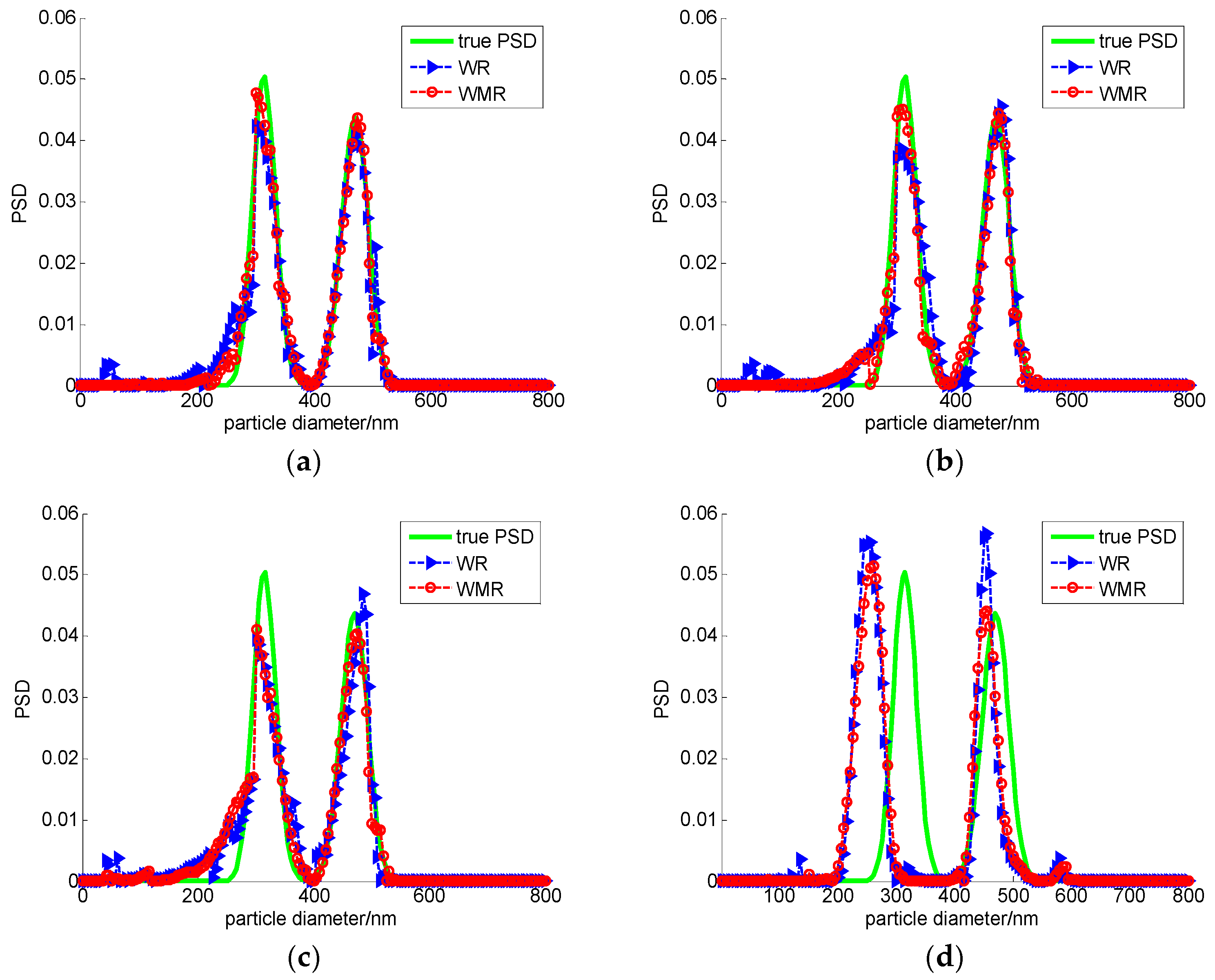
Figure 3.
The inversion results with WR and WMR from 324/601/871 nm trimodal simulated DLS data under different noise levels: (a) noise level is 0; (b) noise level is 10−4; (c) noise level is 10−2; (d) noise level is 0.08.
Figure 3.
The inversion results with WR and WMR from 324/601/871 nm trimodal simulated DLS data under different noise levels: (a) noise level is 0; (b) noise level is 10−4; (c) noise level is 10−2; (d) noise level is 0.08.
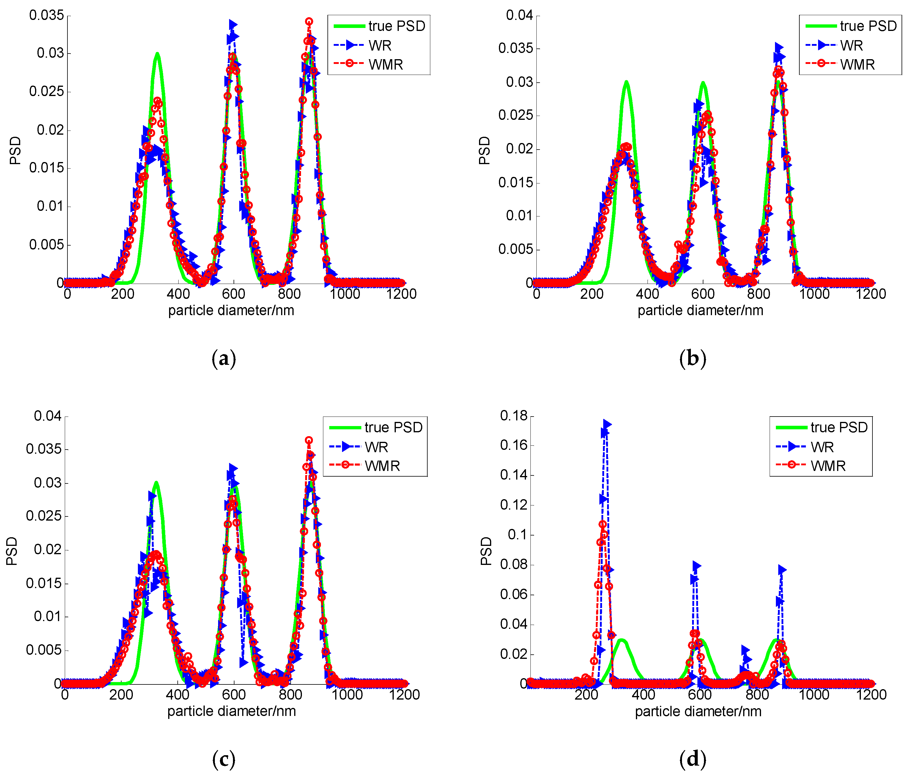
Figure 4.
The inversion results with WR and WMR method from experimental DLS data: (a) 306/974 nm bimodal particles; (b) 300/502 nm bimodal particles.
Figure 4.
The inversion results with WR and WMR method from experimental DLS data: (a) 306/974 nm bimodal particles; (b) 300/502 nm bimodal particles.

Table 1.
Parameters of simulated polydisperse PSD data sets.
| Sample | d1 | d2 | d3 | µ1 | µ2 | µ3 | σ1 | σ2 | σ3 | a | b | c |
|---|---|---|---|---|---|---|---|---|---|---|---|---|
| AS | 466 | 915 | - | 3 | −6 | - | 6.76 | 5.1 | - | 0.5 | 0.5 | - |
| BS | 316 | 470 | - | 4.1 | −3.1 | - | 9.7 | 8.5 | - | 0.5 | 0.5 | - |
| CS | 324 | 601 | 871 | 7.0 | −1 | −7 | 7.2 | 9.05 | 7.2 | 1/3 | 1/3 | 1/3 |
| Unit | μm | μm | μm | - | - | - | - | - | - | - | - | - |
Table 2.
The performance indices of the inversion for simulated 466/915 nm bimodal DLS data under different noise levels.
Table 2.
The performance indices of the inversion for simulated 466/915 nm bimodal DLS data under different noise levels.
| Size/nm | Noise Level | WR | WMR | ||||
|---|---|---|---|---|---|---|---|
| V1 | Pmeas/nm | V2 | V1 | Pmeas/nm | V2 | ||
| 466/915 | 0 | 0.0252 | 451/474/923 | 0.0322/0.0172/0.0087 | 0.0195 | 474/923 | 0.0172/0.0087 |
| 10−4 | 0.0231 | 459/923 | 0.0150/0.0087 | 0.0229 | 459/930 | 0.0150/0.0164 | |
| 10−2 | 0.0349 | 481/923 | 0.0322/0.0087 | 0.0254 | 459/923 | 0.0150/0.0057 | |
| 0.08 | 0.1551 | -/908 | -/0.0076 | 0.1297 | 425/908 | 0.0880/0.0076 | |
Table 3.
The performance indices of the inversion for simulated 316/470 nm bimodal DLS data under different noise levels.
Table 3.
The performance indices of the inversion for simulated 316/470 nm bimodal DLS data under different noise levels.
| Size/nm | Noise Level | WR | WMR | ||||
|---|---|---|---|---|---|---|---|
| V1 | Pmeas/nm | V2 | V1 | Pmeas/nm | V2 | ||
| 316/470 | 0 | 0.0422 | 301/475 | 0.0475/0.0106 | 0.0286 | 301/475 | 0.0475/0.0106 |
| 10−4 | 0.0480 | 306/480 | 0.0316/0.0213 | 0.0380 | 311/475 | 0.0158/0.0106 | |
| 10−2 | 0.0576 | 301/485 | 0.0475/0.0319 | 0.0500 | 301/475 | 0.0475/0.0106 | |
| 0.08 | 0.2113 | 251/455 | 0.2057/0.0319 | 0.1997 | 261/455 | 0.1741/0.0319 | |
Table 4.
The performance indices of the inversion for simulated 324/601/871 nm trimodal DLS data under different noise levels.
Table 4.
The performance indices of the inversion for simulated 324/601/871 nm trimodal DLS data under different noise levels.
| Size/nm | Noise Level | WR | WMR | ||||
|---|---|---|---|---|---|---|---|
| V1 | Pmeas/nm | V2 | V1 | Pmeas/nm | V2 | ||
| 324/601/871 | 0 | 0.0481 | 324/594/878 | 0/0.0116/0.0116 | 0.0326 | 324/594/871 | 0/0.0116/0 |
| 10−4 | 0.0487 | 316/586/608/871 | 0.0247/-/0.0116/0 | 0.0421 | 324/616/871 | 0/0.0250/0 | |
| 10−2 | 0.0523 | 309/339/594/870 | 0.0463/-/0.0116/0.0011 | 0.0419 | 324/594/863 | 0/0.0116/0.0092 | |
| 0.08 | 0.3160 | 271/586/885 | 0.1636/0.0249/0.0161 | 0.2340 | 256/586/885 | 0.2098/0.0249/0.0161 | |
Table 5.
The performance indices of the inversion for experimental DLS data.
| Size/nm | WR | WMR | ||
|---|---|---|---|---|
| Pmeas/nm | V2 | Pmeas/nm | V2 | |
| 306/974 | 313/874 | 0.0228/0.1027 | 301/886 | 0.0196/0.0903 |
| 300/502 | 280/490 | 0.0667/0.0239 | 290/500 | 0.0333/0.004 |
© 2018 by the authors. Licensee MDPI, Basel, Switzerland. This article is an open access article distributed under the terms and conditions of the Creative Commons Attribution (CC BY) license (http://creativecommons.org/licenses/by/4.0/).
Share and Cite
MDPI and ACS Style
Chen, W.; Xiu, W.; Shen, J.; Zhang, W.; Xu, M.; Cao, L.; Ma, L. Multiple-Penalty-Weighted Regularization Inversion for Dynamic Light Scattering. Appl. Sci. 2018, 8, 1674. https://doi.org/10.3390/app8091674
AMA Style
Chen W, Xiu W, Shen J, Zhang W, Xu M, Cao L, Ma L. Multiple-Penalty-Weighted Regularization Inversion for Dynamic Light Scattering. Applied Sciences. 2018; 8(9):1674. https://doi.org/10.3390/app8091674
Chicago/Turabian StyleChen, Wengang, Wenzheng Xiu, Jin Shen, Wenwen Zhang, Min Xu, Lijun Cao, and Lixiu Ma. 2018. "Multiple-Penalty-Weighted Regularization Inversion for Dynamic Light Scattering" Applied Sciences 8, no. 9: 1674. https://doi.org/10.3390/app8091674
Note that from the first issue of 2016, this journal uses article numbers instead of page numbers. See further details here.