A Simplified Methodology to Evaluate the Design Specifications of Hydraulic Components
by
 , , and
Pedro Roquet
1, 
Pedro Javier Gamez-Montero
2,
Robert Castilla
2 ,
,
Gustavo Raush
2 and
Esteban Codina
2,* 1
ROQCAR SL, Antonio Figueras 68, 08551 Tona, Spain
2
Department of Fluid Mechanics, LABSON, Universitat Politecnica de Catalunya, Campus Terrassa, Colom 7, 08222 Terrassa, Spain
*
Author to whom correspondence should be addressed.
Appl. Sci. 2018, 8(9), 1612; https://doi.org/10.3390/app8091612
Submission received: 29 July 2018
/
Revised: 30 August 2018
/
Accepted: 6 September 2018
/
Published: 11 September 2018
(This article belongs to the Special Issue Power Transmission and Control in Power and Vehicle Machineries)
Abstract
:The fatigue of a hydraulic component inherently varies due to various factors that can be divided into two categories: structural and load spectrum variability. The effects of both variabilities must be considered when determining fatigue life. Compared with the structural variability, determining the variability in the load spectrums is more difficult because the service conditions are complicated and the measurements of the load parameters are slow and expensive. The problem that arises when studying the fatigue behaviour of such components is the transferability of short data samples from real-life load histories, which are application-dependant, to laboratory test methods. Derived from the experimental background and know-how of the authors, this paper proposes a methodology that allows the definition and establishment of the hydraulic cylinder design specificactions, while taking into account the probabilistic characterisation of the load spectrum variability. This methodology could be extrapolated to other hydraulic or mechanical components.
1. Introduction
In this paper, we consider a hydraulic cylinder as a typical hydraulic component. Hydraulic cylinders obtain their power from pressurised oil. Hydraulic cylinders are frequently found in equipment and machinery, such as construction equipment (excavators, bull-dozers, and road graders) and material handling equipment (fork lift trucks, telescopic handlers, and lift gates). The cylinder is prone to structural problems, such as buckling and fatigue failure. Until recently, engineers had to choose hydraulic cylinders based on the required pressure range without any accurate life cycle data, and previous service experience was often an indirect validation of the design solution. An example of this is the DNVGL-CG-0194 guideline [1]. This class guideline provides the requirements upon which DNV bases the certification of hydraulic cylinders, including requirements for documentation, design, manufacturing, and testing.
However, these guidelines are no longer sufficient. The hydraulic components are subject to complex and random loads, which determine the reliability of the fatigue and the useful life of the machinery. Therefore, the life reliability must be analytically evaluated to full expected laboratory test specifications. This paper demonstrates how to define these particular specifications according to real load histories.
Reliability is a property expressed as the probability that the component will perform its function without breakdown when operated at a duty cycle and exposed to a specific environment for a given period of time. The reliability must be established during the design phase of the system. It is not a new concept but has created new challenge for hydraulic system designers.
The fatigue of a hydraulic component varies inherently due to various factors that can be divided into two categories: load spectrum and structural variability. The variability of the load spectrum of mobile machinery refers to the differences in the pressure history between hydraulic components of the same type and use. Variability can occur due to differences in machine operator experience, work, trajectory, and so on. Structural variability refers to the statistical variability inherent in the fatigue performance of built-up structures, which arises from the variability in manufacturing technologies and material properties, and is usually quantified by the probability distribution of the fatigue life under prescribed specifications for laboratory tests.
Generally, the hydraulic cylinder design includes basic and detailed stages. During the basic design, the principal dimensions of the rod and tube are determined by considering the working force, speed, and range in terms of yield and buckling. During the detailed design, the dimensions of the rod notch, ports, welds, tube end, gland, and cushion ring are determined by considering the fatigue specifications.
Engineering researchers have strived to obtain standard histories that can be applied efficiently to fatigue analysis as representative of the whole loading process of the target system. The automobile and aerospace industries have developed standard load-time histories (SLHs) that may be applied to different structural or mechanical parts of vehicles and airplanes. The acronym SLH is generally used for standardised load-time histories as well as for standardised load sequences, including load spectra. An extensive list of such waveforms used in industrial laboratories and research centers together with their characteristics and the range of application were presented by Heuler and Klätschke [2]. Unfortunately, this type of standardised load-time histories is not available for mobile machinery, both off-road and agricultural.
In order to assess the fatigue damage of hydraulic components, two different approaches can be used. If the load time history can be captured and recorded easily by experimental measurements or numerical simulation, the time domain fatigue damage assessment approach can be applied. In this approach, all input loading and output stress or strain responses are time-based signals [3,4,5,6]. In other situations, response stress and input loading are preferably expressed as frequency-based signals, usually in the form of power spectral density (PSD). The frequency domain analysis based on the so-called spectral approach is popular. This approach provides a solution to the random vibration fatigue problem, which, in general, is different from our case [7].
Given the aforementioned issues, this paper proposes a methodology that allows the evaluation and definition of hydraulic cylinder design specificactions, taking into account the probabilistic characterisation of the load spectrum variability. The method also provides a simple procedure for the transferability of data from real-life load histories (application-dependant) to laboratory testing methods. The approach used is based on cycle counting schemes and damage accumulation models, such as the reservoir count method and the Palmgren-Miner linear damage rule [8]. These schemes and models are efficient in terms of testing time, effectiveness, and cost.
2. Pressure: Load History and Damage Factor
Our main example for measuring time-load history and then performing statistical analysis is a front loader. In practice, a long-term load spectrum contains complete load information, but this is difficult to directly measure due to the restrictions of testing technology, as well as time and cost. Therefore, obtaining long-term load spectrum information based on short-term data was necessary. Until now, engineers have used traditional methods to obtain long-term load spectrum data, basically consisting of multiplying a short-term load spectrum by a constant proportionality coefficient. The disadvantages of traditional methods are that only the data measured in a finite time are repeated, extreme loads cannot be measured, and their impact on damage is ignored. Load extrapolation methods can overcome the above limitations. With the development of statistics and computer software, although difficult, it is possible to apply load extrapolation methods. Wang et al. [9] provided a selection guidance and several load extrapolation methods that can be applied.
In this paper, an approach inspired by traditional methods is presented to overcome these challenges, consisting of (i) evaluating the damage produced in the hydraulic component for each short-term spectra (damage factor); (ii) considering each short-term spectra and its damage index as statistical samples of the total damage produced by complete load information; and (iii) the laboratory specifications are estimated from the damage factors of different machine tasks, which produce the same damage the component suffers during its lifespan. For illustrative purposes, two front loader tasks were considered: loading and transport. Pressure histories (traces) for all hydraulic cylinders can be obtained by pressure transducers installed in cylinder’s ports.
Current design methods use cycle counting in order to interpret the varying pressure range of the varying loads. The following two methods are the most commontly applied methods in the field of fatigue studies: reservoir and rain-flow. In our case, the obtained data (pressure vs. time) from every pressure trace were treated with the reservoir cycle counting method recommended in EN 13445-3 standard—Unfired pressure vessels Part 3: Design [10]. Also, this algorithm was standardised according to ASTM E 1049-85, Cycle Counting in Fatigue Analysis [8].
Once the cycles were identified, the damage for all the cycles in the loading history were combined to obtain the damage for the entire loading history. A number of deterministic damage accumulation models have been developed since the late 1990, that can be mainly classified into two categories: linear damage cumulative theories [11] and nonlinear damage cumulative theories [12]. The first models have some shortcomings: (i) they fail to consider load history; (ii) cumulative damage has no relationship with load sequence effects; and (iii) effects of load interaction are not taken into account. Therefore, to address the above-mentioned disadvantages, nonlinear cumulative damage theories were suggested, which were classified into six groups by Zhu [13]. Although we are aware that the linear method of mining is non-conservative, it was used because Miner’s rule [14] is probably the simplest and conceptual cumulative damage model that can be used to didactically explain our approach. Miner’s rule states that if there are different pressure levels (with linear damage hypothesis), the fraction of life consumed (damage) D by exposure to the cycles at the different pressure levels is
where is the number of cycles accumulated at pressure Pi and is the number of cycles to failure at pressure Pi.
Fatigue damage for an individual cycle is the reciprocal of the fatigue life, Fatigue lives for a cycle are computed using constant amplitude methods with the appropriate pressure or stress ranges, mean stresses, and material properties. Damage is then summed for all cycles in the loading history.
What should the damage be at failure? If damage were truly a linear process, the damage at failure would be equal to 1. In simple two step block loading, a sequence of high amplitude cycles followed by low amplitude cycles has a damage sum D < 1.0. Similarly, a sequence of low amplitude cycles followed by high amplitude cycles ha a damage sum D > 1.0. In our case, as the succession of peaks of low and high amplitude were randomly distributed, we considered that D ~ 1.0.
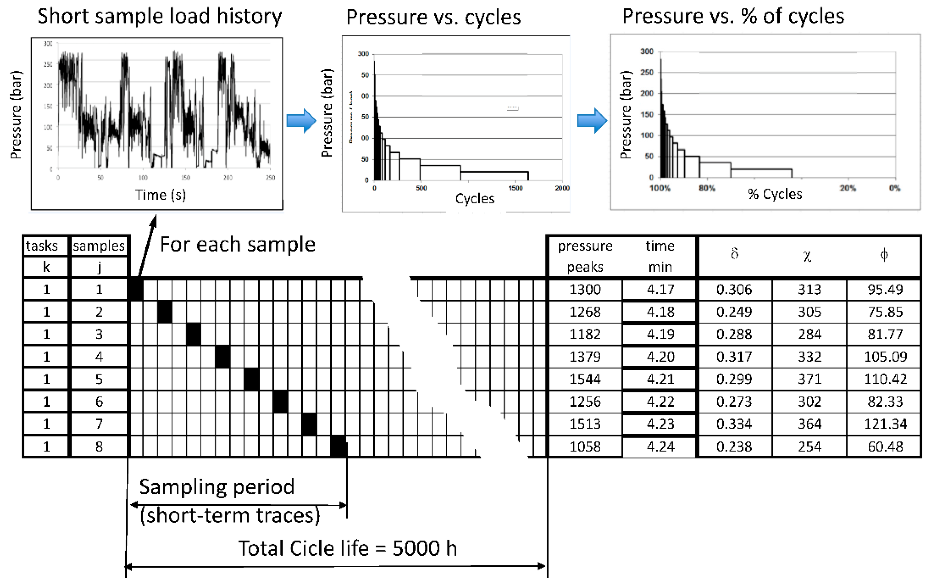
From the pressure spectrum vs. percent cycles (Figure 1), the step damage for every pressure step of the spectrum(εi) can be defined as
where εi is the spectrum relative damage for the ith pressure step of a task, νi is the portion of the task in unified percentage during the Pi pressure level, m is the material coeficient from Basquin equation (m = 3 for steel for hydraulic cylinders [10]), Pi is the pressure value assigned to the ith pressure step of a task, and i is the index that identifies the pressure step number.
The spectrum relative damage (δk) is defined as the sum of all step damages (εi) for this spectrum
where k is the index that identifies the task number.
Although the spectrum relative damage (δk) provides a quantification of the severity of the kth task, it does not take into account the loading frequency. The damage factor (k) is defined as the multiplication of the relative damage factor () by the frequency of the application pressure cycles, (). This frequency is defined as the number of pressure peaks in a time unit.
At this point, only the damage of one portion of the work performed by the machine was calculated (task k). Following the steps described above, it was possible to calculate the damage generated to the hydraulic components by the other tasks.
To illustrate the method, Figure 1 shows eight recorded trace samples (j = 8) that represent the load spectrum variability. From each trace, the pressure spectrum (200 steps are recommended) and the associated damage factor were calculated [15].
Table 1 and Figure 2 show that the statistical distribution (variability) of the damage factors for the task k = 1 (loading task) follows a log-normal distribution where is the accumulated frequency.
The damage factor statistical distribution for k = 1 (loading task) is
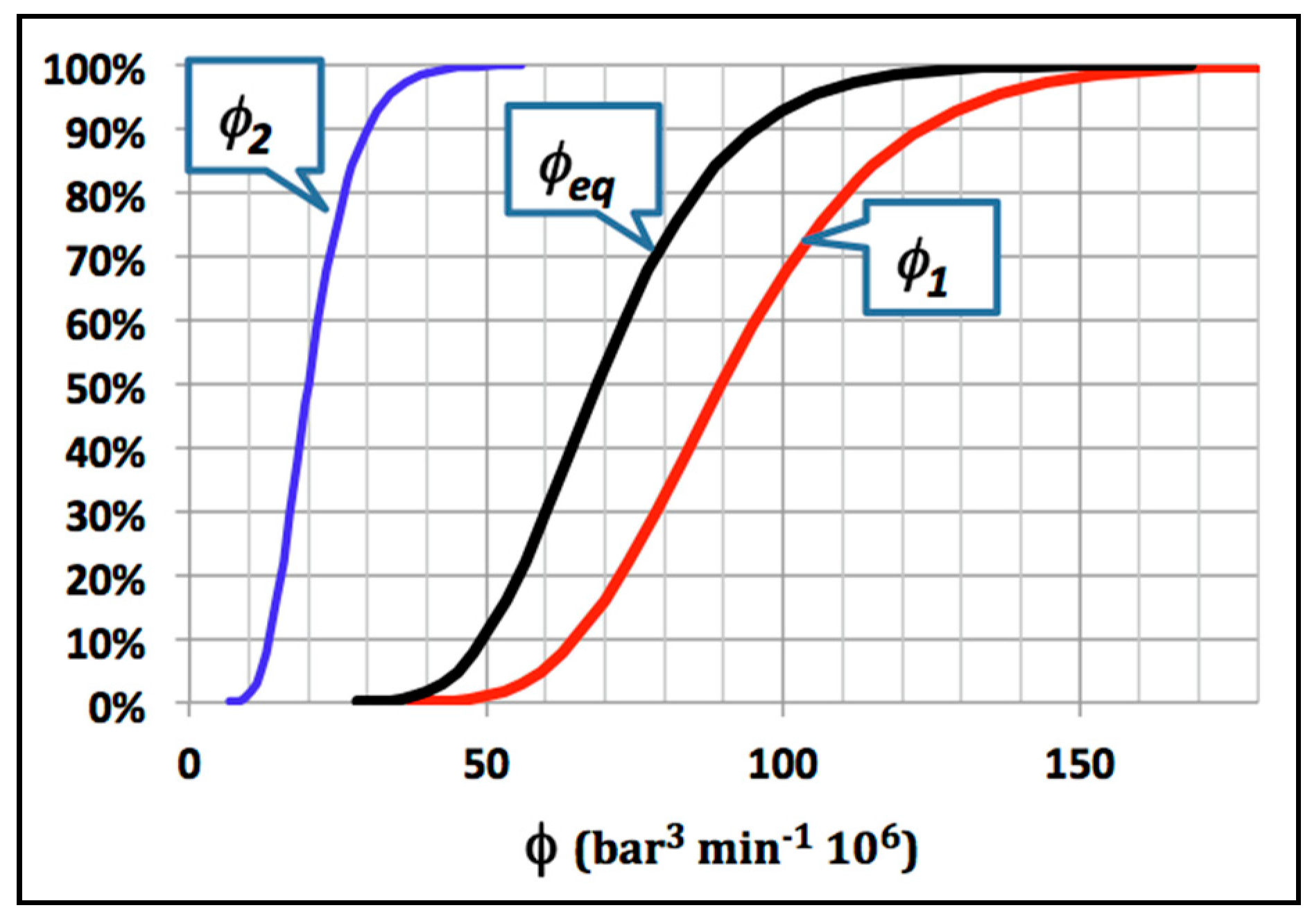
Following the same process, the statistical distributions of the other tasks were calculated. For the task k = 2 (transport task), the following statistical distribution was considered:
To estimate the equivalent damage produced in the cylinder during the full life, we worked with the following data supplied by the machine manufacturer (Table 2).
The equivalent damage factor can be obtained as the sum of the damage factors for all the tasks weighted by a time factor as follows:
Figure 3 shows the statistical distributions of the damage factors of the two considered tasks, as well as the statistical distribution of the equivalent damage. This statistical distributio follows the log-normal type, given that the sum of two (or more) log-normal random variables approaches a log-normal distribution [16].
3. Pressure Specifications
Commonly, the market defines machine life expectancy using different modes, but always specifying working hours, such as 5000 h without failures. More often, statistical concepts are considered, so the life expectancy is expressed as “5000 h β10” [17]. The latter means that when a sampling of 100 machines are tested over 5000 h, only 10 of them (10%) are expected to fail before reaching those working hours. Therefore, the damages generated during the useful life of the machine, when the identified tasks are performed by the machine, cannot generate a failure before the life of the objective T. This can be stated as
which is analogous to the Basquin equation. Then,
where is the Basquin coefficient and Neq is the equivalent number of cycles at a pressure level Peq under constant amplitude conditions.
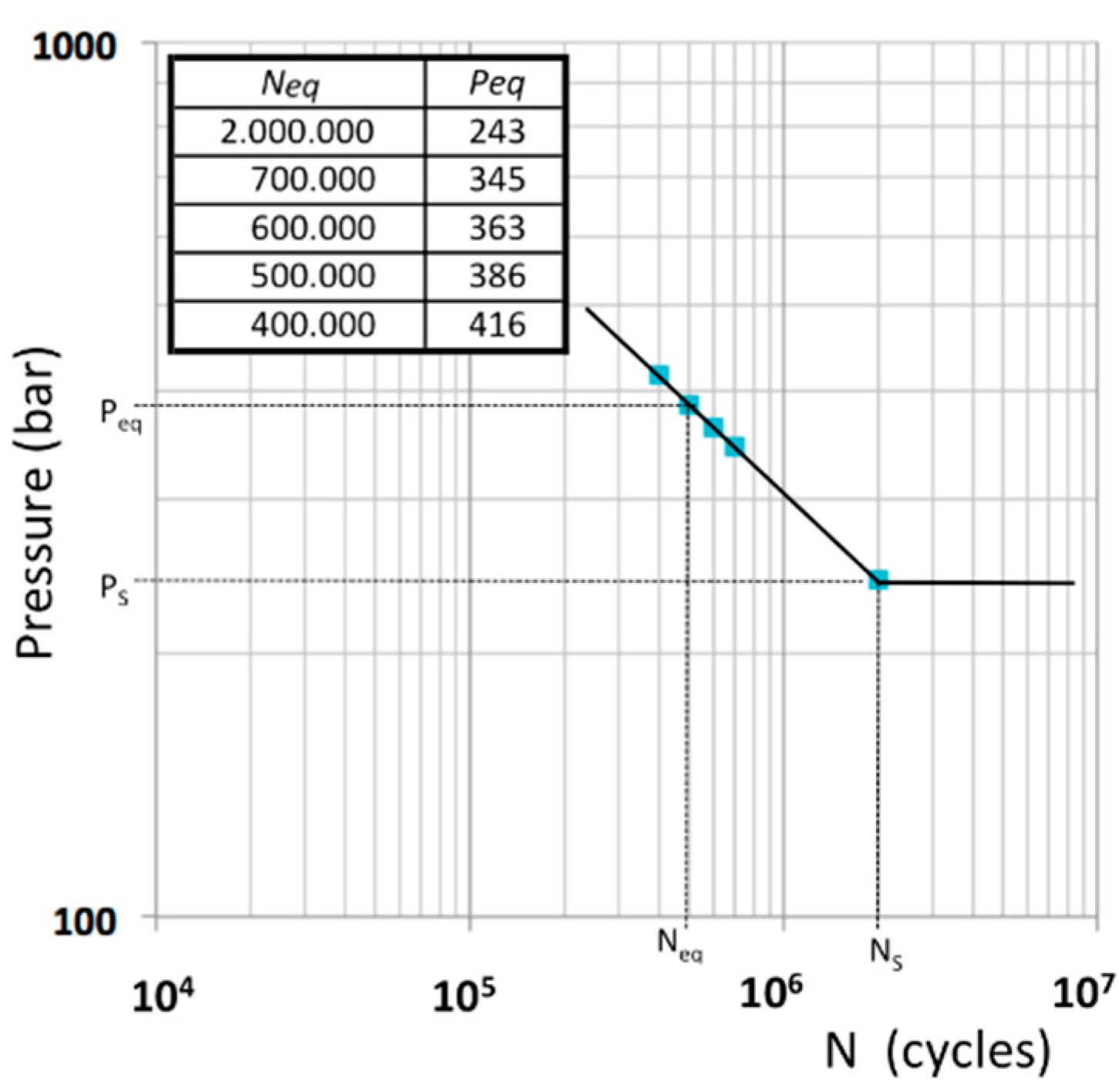
The pair of values (Neq, Peq) defines a line in logarithmic coordinates with slope m (for steel m = 3). From this curve and analogous to what is proposed in standard ISO 13445-3 [9], the curve (Neq, Peq) is identified by equivalent pressure value corresponding to 2 × 10⁶ cycles, which constitutes the class curve :
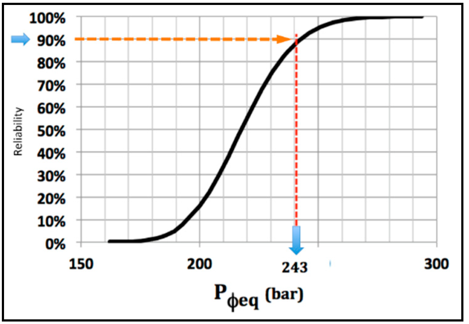
values also follow a log-normal distribution,
At this step, once the statistical distribution of load is known, according to the desired or accepted reliability value, the machine manufacturer may define hydraulic cylinder pressure life specification (laboratory). As an example, if we considered a load reliability of 90%, then (see Figure 4),
The specified pressure PS defines the equivalent damage produced in laboratory test. So, laboratory test parameters (Peq, Neq) that produce an equivalent damage in the cylinder are any values according to Equation (13):
Figure 5 shows that any values of (Peq, Neq) fulfills the specification conditions and produces equal damage to the cylinder (i.e., 386 bar over 500,000 cycles).
.
4. Reliability of Hydraulic Component
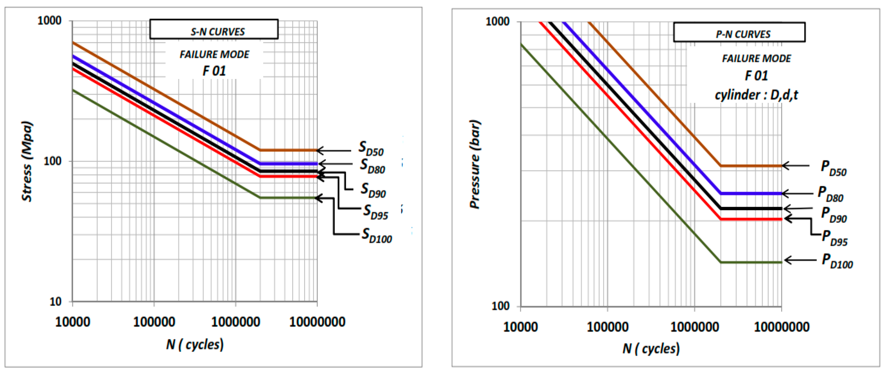
Once the load variability is defined, the structural variability of the hydraulic component is considered. Assuming that a hydraulic component manufacturer knows the S–N curves corresponding to any main possible failure modes and according to its know-how (design and manufacturing technology), determining the fatigue resistance reliability of a hydraulic component is possible. Figure 6 shows the typical S–N curves and corresponding P–N curves for a specific cylinder geometry for the same failure mode (F-01) defined by the value of the pressure PD (or stress SD), which correspond to N = 2 × 10⁶ cycles and nn % of reliability (known as the pressure class nn, or stress class nn of the curve) [10].
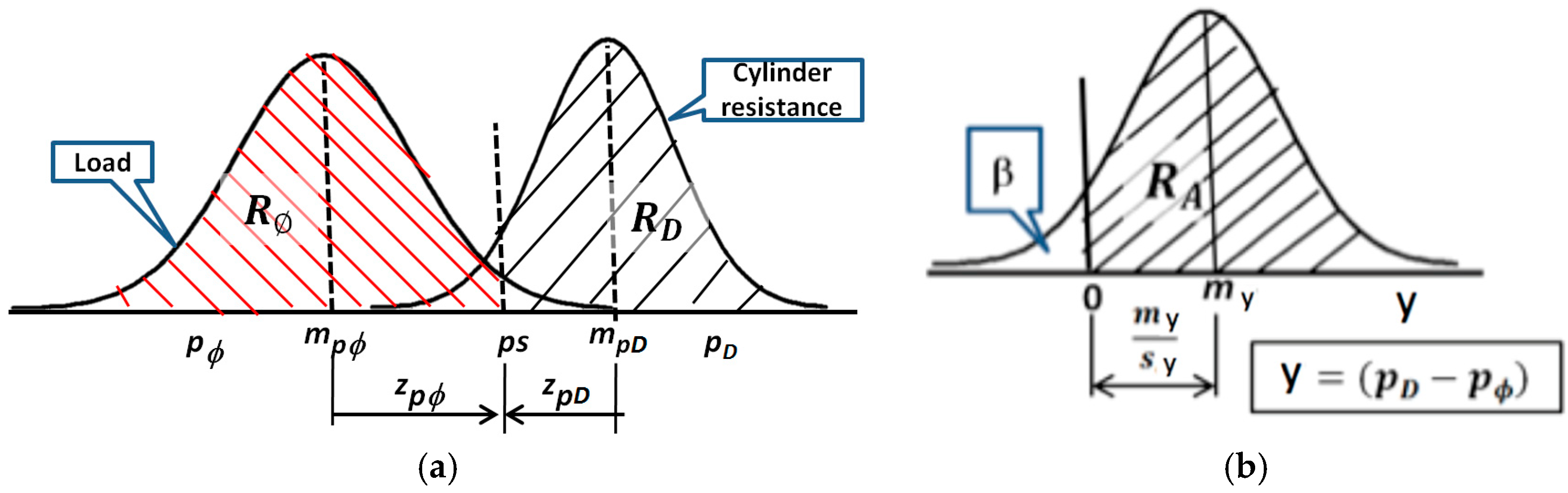
Recalling that fatigue damage due to load conditions is represented by , and damage resistance of the hydraulic cylinder is represented by PD:
Both distributions have PS as a common linkage, which meets the conditions
Any cylinder with a resistance PD may be mounted in a machine with any of the loads . The condition for the cylinder to resist is set by the resistance that is superior to the load (see Figure 7).
The variable y follows a normal distribution:
where
fulfilling
The design data is β = (1 RA), which means “at the end of the life (desired) will not fail more than β% of cylinders”.
If we consider
then,
Equation (22) allows us to estimate the life expectancy, defined by reliability RA, (or the design data β) as a function of load spectrum variability (defined by the reliability, ), resistance variability of the hydraulic component (defined by the reliability, RD) and standard deviation ratio, ks. In practice, the load standard deviation () is known according the proposed approach, but the resistance standard deviation of the hydraulic cylinder () and consequently, the value of the ratio ks cannot be known at the design stage because, sometimes, the selected cylinder manufacturer is still not known. In Table 3, RD values have been tabulated applying Equation (22), see diagram Figure 8, for values within the following ranges: , , and .
Let’s see an example, to satisfy the specifications indicated in Section 3. If β = 10%, (equivalent RA = 90%) and admitting that the load reliability is , Table 3 allows infering that it must demand a hydraulic cylinder resistance variability larger than 84% (for the assumption that ks = 0.25) or larger than 62% (for the assumption that ks = 2). Adopting a conservative position, it leads to demand a minimum resistance reliability of the hydraulic cylinder RD = 85%.
5. Conclusions
Reliability assessment in fatigue failures is a difficult problem: the structural area due to the large scatter in fatigue life and the load history due to highly varying machine user profiles. On one hand, an assessment procedure must therefore be simple enough to be able to quantify vague input information; on the other hand, it must be sophisticated enough to be a useful engineering tool for improvements.
Earlier models of fatigue damage accumulation reported in literature focus on deterministic nature of the process whereas in practice, damage accumulation is of stochastic nature. The main differences in the present method compared to the reported ones are [3,12] that (i) it uses random variables to include the stochasticity in both external loadings and material properties and (ii) the quality of the hydraulic component is represented by the reliability values.
In literature, some similar approaches to the probabilistic damage accumulation paradigm can be found. Shen et al. [18] developed a probabilistic distribution model of stochastic fatigue damage, wherein they have considered the randomness of loading process as well as the randomness of fatigue resistance of material by introducing a random variable of single cycle fatigue damage. Liu and Mahadevan [19] proposed a general methodology for stochastic fatigue life under variable amplitude loading by combining a nonlinear fatigue damage accumulation rule and stochastic S–N curve representation technique. These models are conceptually in the vein of the approach presented in this work. Nevertheless they are more complex and none of them explained how to define the specifications of a component based on the required reliability or a specific algorithm for component reliability prediction.
The major limitation of our approach is that it treats damage accumulation as linear phenomenon (both laboratory and fields tests). It is known that the application of Miner’s rule for variable amplitude life calculation is erroneous. Its effect is weak, specially for typical random loading [20]. However, as cumulative calculations with such values result only in an estimated fatigue life, they still contain a certain risk due to possible lower real damage sums. Therefore, in the case of safety-critical components, which must never fail, an experimental verification is recommended [21,22].
The methodology presented in this work allows, not only the determination of the hydraulic cylinder pressure specifications for laboratory tests, but also provides a simple and quick method to select a hydraulic cylinder since there is a continuous need to improve the durability requirements of the hydraulics components, making them more correlated to the actual customer needs. The potential here is to differentiate the requirements, for example, allowing the offer of a light-weight hydraulic component for specific demanding applications.
Author Contributions
Conceptualization, P.R. and E.C.; Methodology, P.R. and E.C.; Formal Analysis, P.R., E.C., P.J.G.-M., R.C. and G.R.; Investigation, P.R., E.C., P.J.G.-M., R.C. and G.R.; Writing—Original Draft Preparation, P.R. and E.C.; Writing—Review & Editing, P.J.G.-M.
Funding
The authors disclosed receipt of the following financial support for the research, authorship, and/or publication of this article: This research program has received funding from the European Union Seventh Framework Programme FP6 NMP-CT-2004-505466 ‘New design and manufacturing processes for high pressure fluid power products’ (Acronym: PROHIPP).
Conflicts of Interest
The authors declare no conflict of interest.
Nomenclature
| D | fraction of life consumed (damage) |
| F | accumulate frequency |
| j | trace samples |
| m | material coefficient from Basquin equation |
| ni | number of cycles accumulated at pressure Pi |
| Neq | equivalent number of cycles to failure at pressure Peq |
| Ni | number of cycles to failure at pressure Pi |
| PD | damage resistance of the hydraulic cylinder |
| Pi | pressure level assigned to the ith pressure step of a task |
| PS | equivalent damage produced in laboratory test |
| loads | |
| fatigue damage due to load conditions | |
| RA | life expectancy reliability |
| RD | resistance reliability |
| load reliability | |
| load standard deviation | |
| resistance standard deviation of the hydraulic cylinder | |
| SD | stress |
| T | life objective |
| z | standard normal variable |
Greek Symbols
| α | Basquin coefficient |
| β | live expectancy |
| δi | spectrum relative damage |
| δk | relative damage factor |
| εi | step damage for every pressure step of the spectrum |
| πk | time factor |
| χk | frequency of the application pressure cycles |
| feq | equivalent damage factor |
| fk | damage factor |
References
- Hydraulic Cylinders. Class Guideline DNVGL-CG-0194. Edition July 2017. Available online: https://www.dnvgl.com (accessed on 27 July 2018).
- Heuler, P.; Klätschke, H. Generation and use of standardised load spectra and load-time histories. Int. J. Fatigue 2005, 27, 974–990. [Google Scholar] [CrossRef]
- Johannesson, P.; Speckert, M. Guide to Load Analysis for Durability in Vehicle Engineering; John Wiley & Sons Ltd.: Chichester, UK, 2013; pp. 1–456. ISBN 978-1-118-64831-5. [Google Scholar]
- Johannesson, P. Extrapolation of Load Histories and Spectra. Fatigue Fract. Eng. Mater. Struct. 2006, 29, 209–217. [Google Scholar] [CrossRef]
- Shen, R.; Zhang, X.; Zhou, C. Dynamic Simulation of the Harvester Boom Cylinder. Machines 2017, 5, 13. [Google Scholar] [CrossRef]
- Jerabek, I.; Horky, L.; Weigel, K. Long-term test- analysis and monitoring. In Proceedings of the EAN-55th Conference on Experimental Stress Analysis, Novy Smokovec, Slovakia, 30 May–1 June 2017; Available online: http://experimentalni-mechanika.cz/konference/2017.html?download=1339:long-term-cyclic-test-analysis-and-monitoring (accessed on 15 May 2018).
- Qiang, R.; Hongyan, W. Frequency Domain Fatigue Assessment of Vehicle Component under Random Load Spectrum. J. Phys. Conf. Ser. 2011, 305, 012060. [Google Scholar] [CrossRef] [Green Version]
- ASTM. Standard Practices for Cycle Counting in Fatigue Analysis, Annual Book of ASTM Standards; ASTM E1049-85; ASTM International: West Conshohocken, PA, USA, 2017; Volume 03.01, pp. 710–718. [Google Scholar]
- Wang, J.; Chen, H.; Li, Y.; Wu, Y.; Zhang, Y. A Review of the Extrapolation Method in Load Spectrum Compiling. J. Mech. Eng. 2016, 62, 60–75. [Google Scholar] [CrossRef]
- EN 13445. Unfired Pressure Vessels is a Standard that Provides Rules for the Design, Fabrication, and Inspection of Pressure Vessels; (EN 13445 Consists of 10 Parts). Part 3: Dedicated to Design Rules; 2004; Available online: http://www.unm.fr/main/download.php?file=107_FICHIER_0.pdf (accessed on 27 July 2018).
- Yang, X.H.; Yao, W.X.; Duan, C.M. The development of deterministic fatigue cumulative damage theory. Eng. Sci. 2003, 15, 81–87. [Google Scholar]
- Fatemi, A.; Yang, L. Cumulative fatigue damage and life prediction theories: A survey of the state of the art for homogeneous materials. Int. J. Fatigue 1998, 20, 9–34. [Google Scholar] [CrossRef]
- Zhu, S.P.; Huang, H.Z.; Liu, Y. A practical method for determining the Corten-Dolan exponent and its application to fatigue life prediction. Int. J. Turbo Jet-Engines 2012, 29, 79–87. [Google Scholar] [CrossRef]
- Miner, M.A. Cumulative damage in fatigue. J. Appl. Mech. 1945, 12, 159–164. [Google Scholar]
- Roquet, P.; Codina, E.; Perez, J. Hydraulic Components Fatigue Assessment Based on Real Life Load Histories; Conference TEH2017; INMA Bucharest: Bucarest, Romania, 2017. [Google Scholar]
- Lo, C.F. The Sum and Difference of Two Log-normal Random Variables. J. Appl. Math. 2012, 2012, 1–13. [Google Scholar] [CrossRef]
- Stimson, W.A. Appendix B: Introduction to Product Reliability. In Forensic Systems Engineering: Evaluating Operations by Discovery; John Wiley & Sons Ltd.: Hoboken, NJ, USA, 2018; pp. 1–368. ISBN 978-1-119-42275-4. [Google Scholar]
- Shen, H.; Lin, J.; Mu, E. Probabilistic model on stochastic fatigue damage. Int. J. Fatigue 2000, 22, 569–572. [Google Scholar] [CrossRef]
- Liu, Y.; Mahadevan, S. Stochastic fatigue damage model-ing under variable amplitude loading. Int. J. Fatigue 2007, 29, 1149–1161. [Google Scholar] [CrossRef]
- Vormwalda, M. Classification of load sequence effects in metallic structures. Procedia Eng. 2015, 101, 534–542. [Google Scholar] [CrossRef]
- Gamez-Montero, P.J.; Salazar, E.; Castilla, R.; Freire, J.; Khamashta, M.; Codina, E. Misalignment effects on the load capacity of a hydraulic cylinder. Int. J. Mech. Sci. 2009, 51, 105–113. [Google Scholar] [CrossRef]
- Gamez-Montero, P.J.; Salazar, E.; Castilla, R.; Freire, J.; Khamashta, M.; Codina, E. Friction effects on the load capacity of a column and a hydraulic cylinder. Int. J. Mech. Sci. 2009, 51, 141–151. [Google Scholar] [CrossRef]
Figure 1.
Scheme of load histories sampling and treatment.

Figure 2.
Statistical distribution of damage factor for k = 1 (loading task).
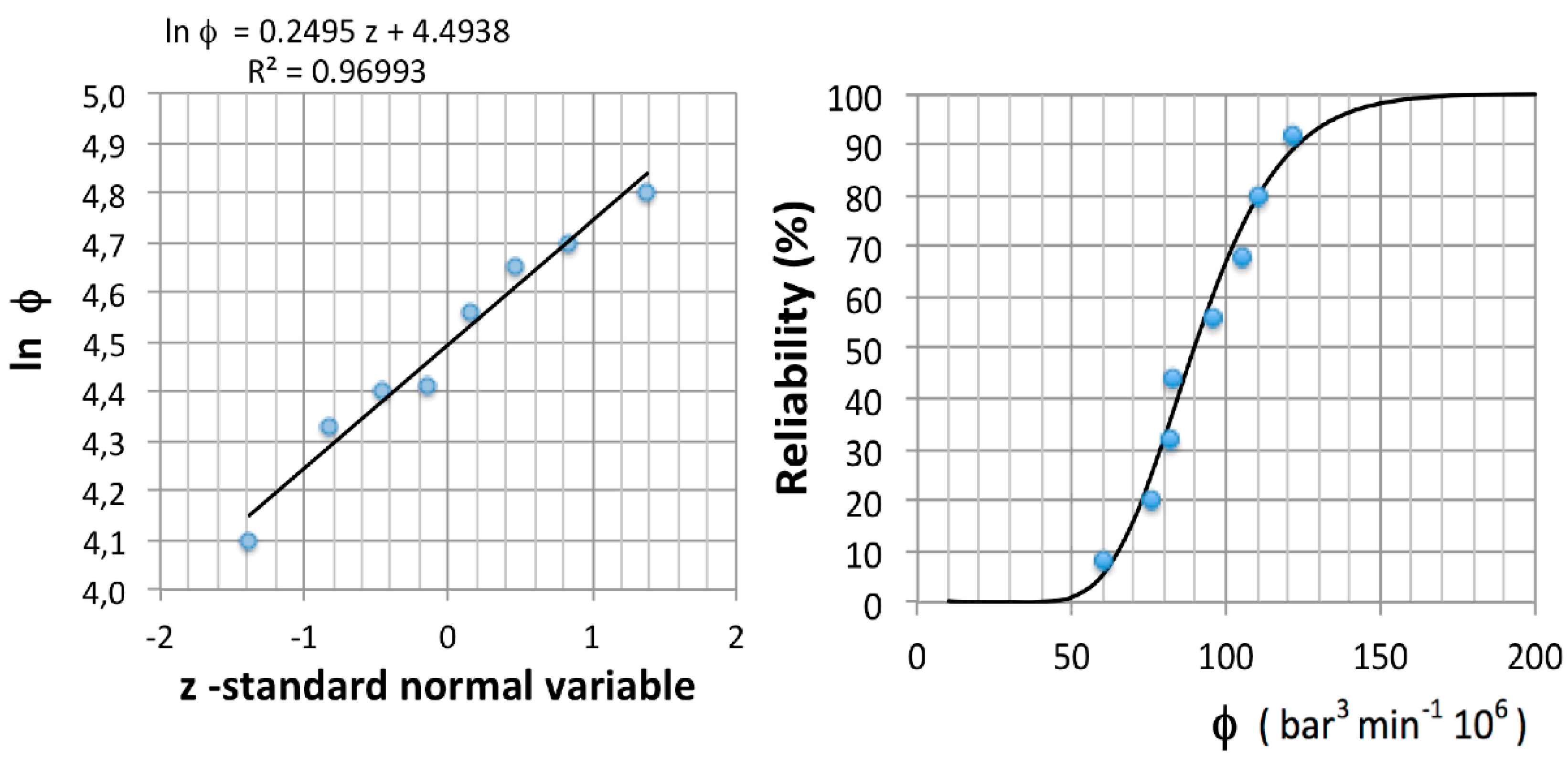
Figure 3.
Statistical distribution of damage factors.

Figure 4.
Statistical distribution of .

Figure 5.
Laboratory test parameters according pressure specifications.

Figure 6.
Typical (left) S–N curves and (right) P–N curves for specific hydrauklic cylinder geometry for this same failure mode (F-01).
Figure 6.
Typical (left) S–N curves and (right) P–N curves for specific hydrauklic cylinder geometry for this same failure mode (F-01).

Figure 7.
Cylinder mounted in a machine with any of the loads: (a) Load variability and structural variability functions; (b) At the end of the life will not fail more than β % of cylinders.
Figure 7.
Cylinder mounted in a machine with any of the loads: (a) Load variability and structural variability functions; (b) At the end of the life will not fail more than β % of cylinders.

Figure 8.
Scheme to calculate the required resistance reliability (RD).


Table 1.
Damage factors for the task k = 1 (loading task).
| k | j | (bar3·min−1·106) | F (%) | ln () | z |
|---|---|---|---|---|---|
| 1 | 8 | 60.48 | 8.3 | 4.10 | −1.38 |
| 1 | 5 | 75.85 | 20.2 | 4.33 | −0.83 |
| 1 | 3 | 81.77 | 32.1 | 4.40 | −0.46 |
| 1 | 6 | 82.33 | 44.0 | 4.41 | −0.15 |
| 1 | 1 | 95.49 | 56.0 | 4.56 | 0.15 |
| 1 | 4 | 105.09 | 67.9 | 4.65 | 0.46 |
| 1 | 5 | 110.42 | 79.8 | 4.70 | 0.83 |
| 1 | 7 | 121.34 | 91.7 | 4.80 | 1.38 |
Table 2.
Cylinder data from the machine manufacturer.
| k | Task | T (Hour) | πk |
|---|---|---|---|
| 1 | Loading | 3500 | 0.70 |
| 2 | Transport | 1500 | 0.30 |
Table 3.
Values of hydraulic cylinder resistance reliability RD.
| Rφ (%) | B (%) | ks 0.25 | ks 0.65 | ks 0.85 | ks 1 | ks 1.5 | ks 2 |
|---|---|---|---|---|---|---|---|
| 50 | 3 | 98 | 99 | 99 | 100 | ||
| 50 | 5 | 96 | 98 | 98 | 99 | 100 | |
| 50 | 10 | 91 | 94 | 95 | 97 | 99 | 100 |
| 80 | 3 | 96 | 96 | 97 | 97 | 99 | 100 |
| 80 | 5 | 93 | 92 | 93 | 93 | 96 | 98 |
| 80 | 10 | 87 | 84 | 83 | 83 | 85 | 88 |
| 85 | 3 | 96 | 95 | 95 | 96 | 98 | 99 |
| 85 | 5 | 92 | 90 | 90 | 90 | 92 | 95 |
| 85 | 10 | 86 | 80 | 79 | 78 | 78 | 79 |
| 90 | 3 | 96 | 93 | 93 | 93 | 95 | 97 |
| 90 | 5 | 92 | 87 | 86 | 85 | 85 | 87 |
| 90 | 10 | 84 | 76 | 72 | 70 | 65 | 62 |
| 95 | 3 | 95 | 90 | 88 | 87 | 86 | 86 |
| 95 | 5 | 90 | 81 | 78 | 75 | 69 | 65 |
| 95 | 10 | 82 | 68 | 61 | 57 | 44 | 34 |
© 2018 by the authors. Licensee MDPI, Basel, Switzerland. This article is an open access article distributed under the terms and conditions of the Creative Commons Attribution (CC BY) license (http://creativecommons.org/licenses/by/4.0/).
Share and Cite
MDPI and ACS Style
Roquet, P.; Gamez-Montero, P.J.; Castilla, R.; Raush, G.; Codina, E. A Simplified Methodology to Evaluate the Design Specifications of Hydraulic Components. Appl. Sci. 2018, 8, 1612. https://doi.org/10.3390/app8091612
AMA Style
Roquet P, Gamez-Montero PJ, Castilla R, Raush G, Codina E. A Simplified Methodology to Evaluate the Design Specifications of Hydraulic Components. Applied Sciences. 2018; 8(9):1612. https://doi.org/10.3390/app8091612
Chicago/Turabian StyleRoquet, Pedro, Pedro Javier Gamez-Montero, Robert Castilla, Gustavo Raush, and Esteban Codina. 2018. "A Simplified Methodology to Evaluate the Design Specifications of Hydraulic Components" Applied Sciences 8, no. 9: 1612. https://doi.org/10.3390/app8091612
Note that from the first issue of 2016, this journal uses article numbers instead of page numbers. See further details here.