Adaptive Impedance-Based Fault Location Algorithm for Active Distribution Networks

Abstract

Modern fault location methods are robust; however, they depend strongly on the availability of the measurements given by Distributed Energy Resources (DER). If the communication or synchronism of this information is lost, the fault location is not possible. This paper proposes an adaptive impedance-based fault location algorithm for active distribution systems. The proposal combines information provided by Intelligent Electronic Devices (IEDs) located at the substation, the knowledge of the network topology and parameters, as well as the distributed power sources, to estimate the fault location. Its adaptive feature is given by the use of a Distributed Energy Resources (DER) electrical model. This model is used to estimate the DER current contribution to the fault, in case the information provided by a local IED is not available. The method takes two types of DER technologies into account: Inverter non-interfaced DER (INIDER) and Inverter-interfaced DER (IIDER). The proposed method is validated on a modified IEEE 34-node test feeder, which was simulated with ATP/EMTP. The results obtained using the IEDs information, presented a maximum error of 0.8%. When this information is not available, the method’s performance decreases slightly, obtaining a maximum error of 1.1%. The proposed method showed better performance when compared with two state of the art methods, indicating potential use for real-life applications.

1. Introduction

Fault location (FL) is one of the most important tasks in the supervision and management of electrical networks with self-healing features. This task plays an important role on the fast maintenance and restoration of the electricity supply for the costumers [1,2]. However, despite technological advancements, the FL process is still based on the calls from customers who provide useful information for identifying the fault region. This procedure proves to be inefficient, since it requires the maintenance team to visually inspect a potentially large region to locate the fault point. Currently, there are several techniques that are based on mathematical formulations proposed for FL estimation. They use information such as the system topology, its electrical parameters, and recorded voltage and currents at the substation [3,4]. Among them, there are methods based on traveling waves, artificial intelligence, and impedance-based methods. Traveling-wave methods for FL have been presented previously [5,6]. These techniques present some limitations, such as the requirement of high sampling rate [3]. On the other hand, artificial intelligence-based methods present a high performance. Still, they need large databases to perform their learning process, and their accuracy depends on the database information quality [3,6,7,8].

The impedance-based methods are one of the most successful techniques for FL [3]. These methods are easy to implement in real life applications, have good precision, and a high cost/benefit relationship [9,10,11,12]. However, these techniques present some limitations like the estimation of multiple FL. This problem can be reduced by artificial intelligence-, traveling waves-, or circuital analysis-based strategies [4,13,14]. Additionally, with the development of smart grids and the use of renewable energy, distribution grids are being transformed from passive to active networks. With this, including the effect of Distributed Energy Resources (DER) on the formulation of the FL problem becomes necessary; DER comprise Distributed Generation (DG) technologies and energy storage technologies [15]. Most DER require a power electronic based interface—defined in this paper as Inverter-interfaced DER (IIDER)—to connect them and ensure their synchronization with the Power Distribution System (PDS). The remaining DER are connected directly to the network, and are defined as Inverter non-interfaced DER (INIDER).

Some strategies to consider the DER effect on FL have been proposed in the technical literature [16,17,18,19,20,21,22,23,24,25,26,27]. In [16,17,25] the DER effect is considered by using a model of the synchronous machine, which is only valid for INIDER [28]. In [26,27] the DER effect is considered by using a model of the inverter, which is only valid for IIDER. Further, the methods exposed in the literature [18,19,20,21,22,23,24] are formulated using synchronized current and voltage phasors, provided by Intelligent Electronic Devices (IED), in order to consider the DER effect on the FL. These methods are robust, but depend strongly on the availability of measurements given by IED, which are installed in DER. If the IED communication or its synchronization with the Distribution Management System (DMS) is lost; the FL is not possible. In this context, it is most important to create models that allow the FL estimation without relying on the availability of measurements on DER location.

Considering such, the main contribution of this work is the development of an adaptive impedance-based FL algorithm for active distribution networks. It combines the information provided by IEDs, located at the substation, and the DER to estimate the FL. Nevertheless, if the information provided by the IED is not available, the DER effect is considered by the use of its equivalent linear analytical models. Two DER electrical models are considered: the approximate model of the synchronous machine for considering the INIDER effect, and the inverter model operating in limiting current to consider the IIDER effect. These models are used to estimate the current contribution from DER units to the fault point. In this work, the fault resistance was considered to be constant over time, and the problem of multiple estimation of FL was not addressed.

The remaining of this paper is organized as follows. Section 2 presents the proposed fault location equations for ground and phase faults. Section 3 presents the proposed adaptive impedance-based fault location algorithm for active distribution systems. Section 4 presents the case study, and Section 5 the results. Section 6 presents the discussion of the results and finally, in Section 7, the main conclusions of this work are presented.

2. Proposed Generalized Fault Location Equations

This work proposes an Adaptive Impedance-Based fault location algorithm for active distribution networks. The proposed method is an extension of the mathematical formulation presented in [11]. Ref. [11] considers typical features of distribution systems for its formulation, such as the unbalanced operation; capacitive effect; single, two-phase, and three-phase laterals; making it a robust fault location method. However, it does not consider the presence of DER.

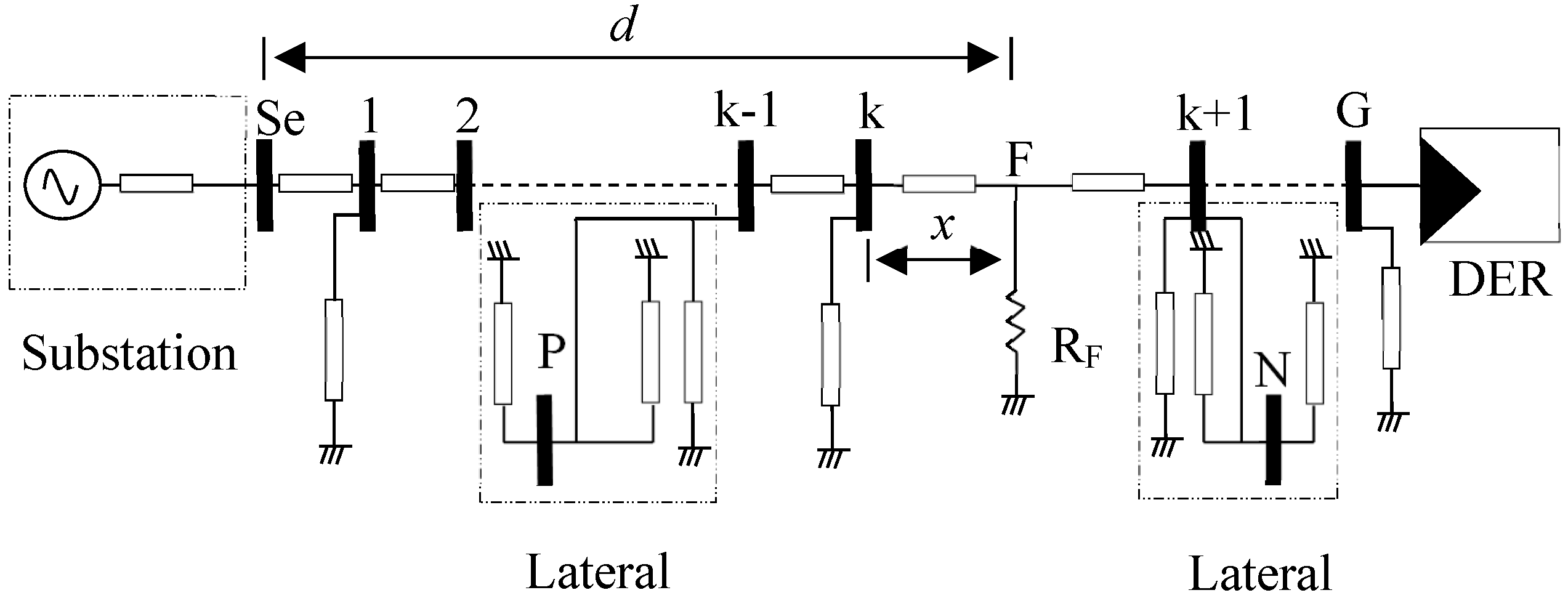
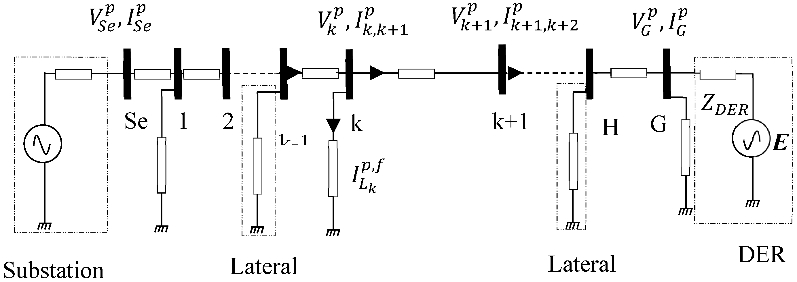
Consider the power distribution system illustrated in Figure 1. This system has a fault between nodes $k$ and $k+1$.

The main objective of a fault location formulation is to estimate the distance d from the substation up to the fault point. Therefore, considering that the fault section is unknown, all sections of the system are assumed in fault and a distance x is estimated for each section. This estimation is made until a convergence criterion is achieved. For this reason, the fault location analysis is reduced to a particular line section.

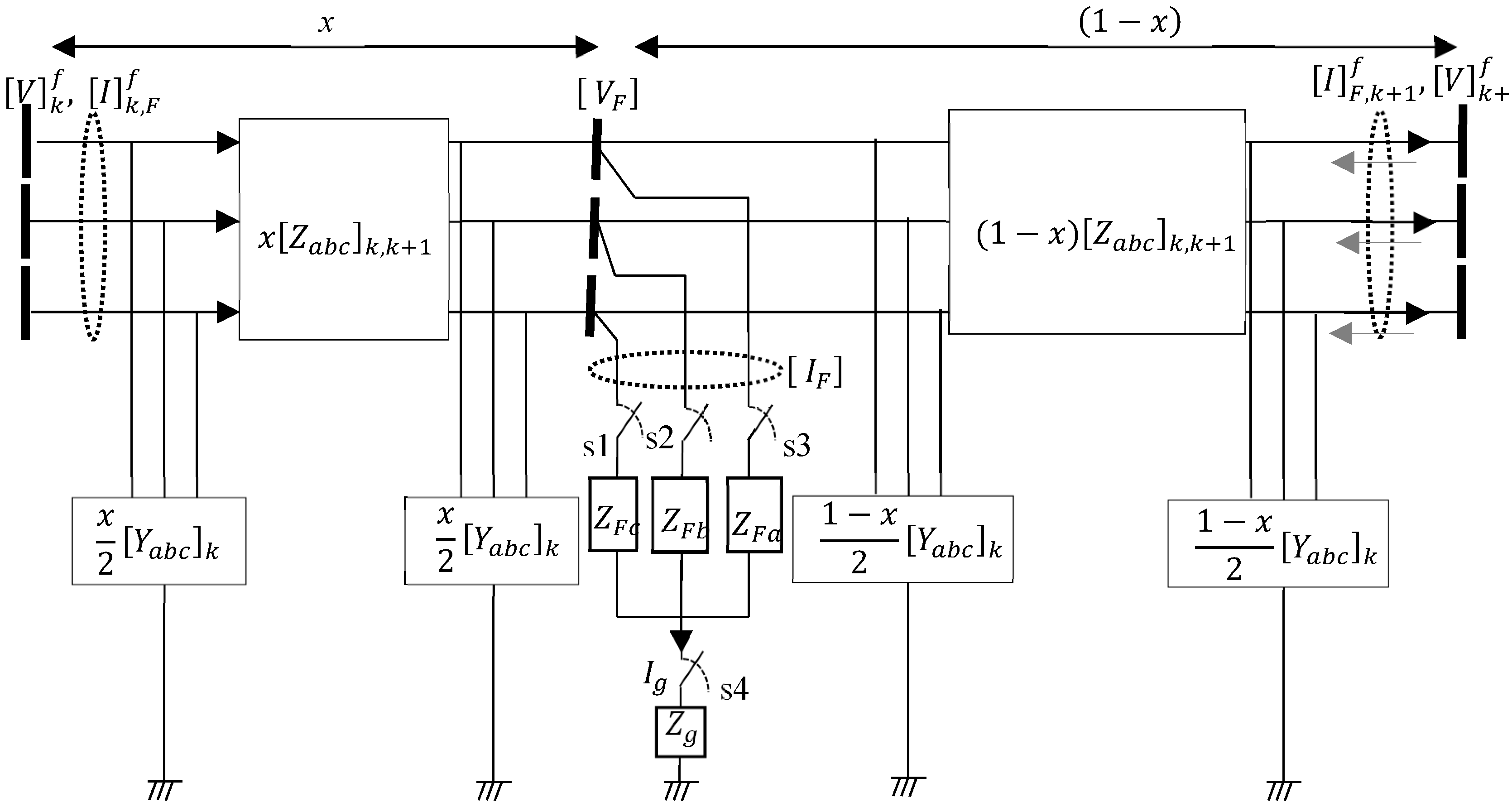
Consider now a distribution line under fault, which is represented by its exact line segment model, as shown in Figure 2. Different types of faults can be obtained from the combination of switches $s1,s2,s3$, and $s4$.

2.1. Ground Faults

Consider the generalized model of a fault illustrated in Figure 2. By modifying the states of the switches $s1,s2$, $s3$, and maintaining switch s4 closed, any phase-to-ground fault type is obtained.

Using this model it is possible to derive [11]:

$$\left[\begin{array}{c}{V}_{F_a}\\ V_{F_b}\\ V_{F_c}\end{array}\right]=\left[\begin{array}{ccc}{Z}_{F_a}+Z_{F_g}& Z_{F_g}& Z_{F_g}\\ Z_{F_g}& Z_{F_b}+Z_{F_g}& Z_{F_g}\\ Z_{F_g}& Z_{F_g}& Z_{F_c}+Z_{F_g}\end{array}\right]·\left[\begin{array}{c}{I}_{F_a}\\ I_{F_b}\\ I_{F_c}\end{array}\right]$$

(1)

In Equation (1), only the faulty phases have fault currents that are different from zero. From Figure 2, an expression for the fault point voltage is obtained, depending on the fault distance.

$${\mathit{V}}_F={\mathit{d}}_x·{\mathit{V}}_k-{\mathit{b}}_x·{\mathit{I}}_{k,F}$$

(2)

where,

$${\mathit{d}}_x=\mathit{I}+0.5·x^2·{\mathit{Z}}_{abc}·{\mathit{Y}}_{abc}$$

(3)

$${\mathit{b}}_x=x·{\mathit{Z}}_{abc}$$

(4)

Replacing Equation (2) in Equation (1), splitting into its real and imaginary parts, and considering $Z_{F_w}$ and $Z_{F_g}$ as pure resistances, a generalized expression for phase-to-ground faults is obtained, as shown by Equation (5).

$$x^2·\left[0.5·{\displaystyle \sum _{w\in {\Omega }_w}}\Im \left\{M_w·I_{F_w}^{*}\right\}\right]-x·\left[{\displaystyle \sum _{w\in {\Omega }_w}}\Im \left\{N_w·I_{F_w}^{*}\right\}\right]+\left[{\displaystyle \sum _{w\in {\Omega }_w}}\Im \left\{V_{k_w}·I_{F_w}^{*}\right\}\right]=0$$

(5)

The variables $M$ and $N$ are defined as:

$$\left[\begin{array}{c}{M}_a\\ M_b\\ M_c\end{array}\right]=\left[\begin{array}{ccc}{Z}_{aa}& Z_{ab}& Z_{ac}\\ Z_{ba}& Z_{bb}& Z_{bc}\\ Z_{ca}& Z_{cb}& Z_{cc}\end{array}\right]·\left[\begin{array}{ccc}{Y}_{aa}& Y_{ab}& Y_{ac}\\ Y_{ba}& Y_{bb}& Y_{bc}\\ Y_{ca}& Y_{cb}& Y_{cc}\end{array}\right]·\left[\begin{array}{c}{V}_{k_a}\\ V_{k_b}\\ V_{k_c}\end{array}\right]$$

(6)

$$\left[\begin{array}{c}{N}_a\\ N_b\\ N_c\end{array}\right]=\left[\begin{array}{ccc}{Z}_{aa}& Z_{ab}& Z_{ac}\\ Z_{ba}& Z_{bb}& Z_{bc}\\ Z_{ca}& Z_{cb}& Z_{cc}\end{array}\right]·\left[\begin{array}{c}{I}_{k,F_a}\\ I_{k,F_b}\\ I_{k,F_c}\end{array}\right]$$

(7)

2.2. Line-To-Line (LL) Faults

Consider the generalized model of a fault illustrated in Figure 2. By modifying the states of the switches $s1,s2$, and $s3$, and maintaining switch S4 open, any line-to-line (LL) fault type can be obtained. According to this model, voltages at the faulted location are estimated according to Equation (9).

$$I_{F_b}=-I_{F_a}$$

(8)

$$V_{F_a}=V_{k_a}+x^2·0.5·M_a-x·N_a=V_{k_b}+x^2·0.5·M_b-x·N_b+Z_F·I_{F_a}$$

(9)

Making the same procedure as for phase-to-ground faults, a generalized expression for line-to-line (LL) faults is achieved, where $u$ and $v$ are faulted phases.

$$x^2·0.5·\Im \left\{\left(M_u-M_v\right)·I_{F_u}^{*}\right\}-x·\Im \left\{\left(N_u-N_v\right)·I_{F_u}^{*}\right\}+\Im \left\{\left(V_{k_u}-V_{k_v}\right)·I_{F_u}^{*}\right\}=0$$

(10)

Equations (5) and (10) are second-order polynomials in $x$; consequently, two solutions are estimated. Thus, the fault distance $x$, which represents the physically correct solution, must be estimated as shown in [11].

The previous analysis allows the fault distance estimation in a line section. However, it is necessary to develop an algorithm which allows its application in each line section of the power distribution system. An algorithm, such as the one presented previously [14], can be used. The limitation of such algorithm is that it does not consider the presence of DER.

Consider now for INIDER, the approximate model of the synchronous machine given by an ideal voltage source that represents the internal voltage of the generator, and the reactance of direct axis during the subtransient period [29,30]. The choice of the subtransient period ensures that the concatenated flows in the rotor remain constant, as well as the internal voltage of the machine between the period of prefault and the time taken for analysis in the fault [17,29,30]. Therefore, the machine’s prefault period internal voltage is estimated. In the case that the reactance is not known, typical values reported in the technical literature can be used [31]. The knowledge of the internal voltage in the DG model allows modeling its behavior in the fault period. This enables the estimation of the current contribution to the fault point by the application of circuit reduction theorems such as the Thevenin’s theorem [16].

Similarly, IIDER are considered in this method by including the fault response model of the inverter operating in current limiting mode. In this case, DER are represented as a voltage source and an impedance, which are defined in function of the saturation current of the inverter and the filter parameters [27].

3. Adaptive Fault Location Algorithm for Active Distribution Systems

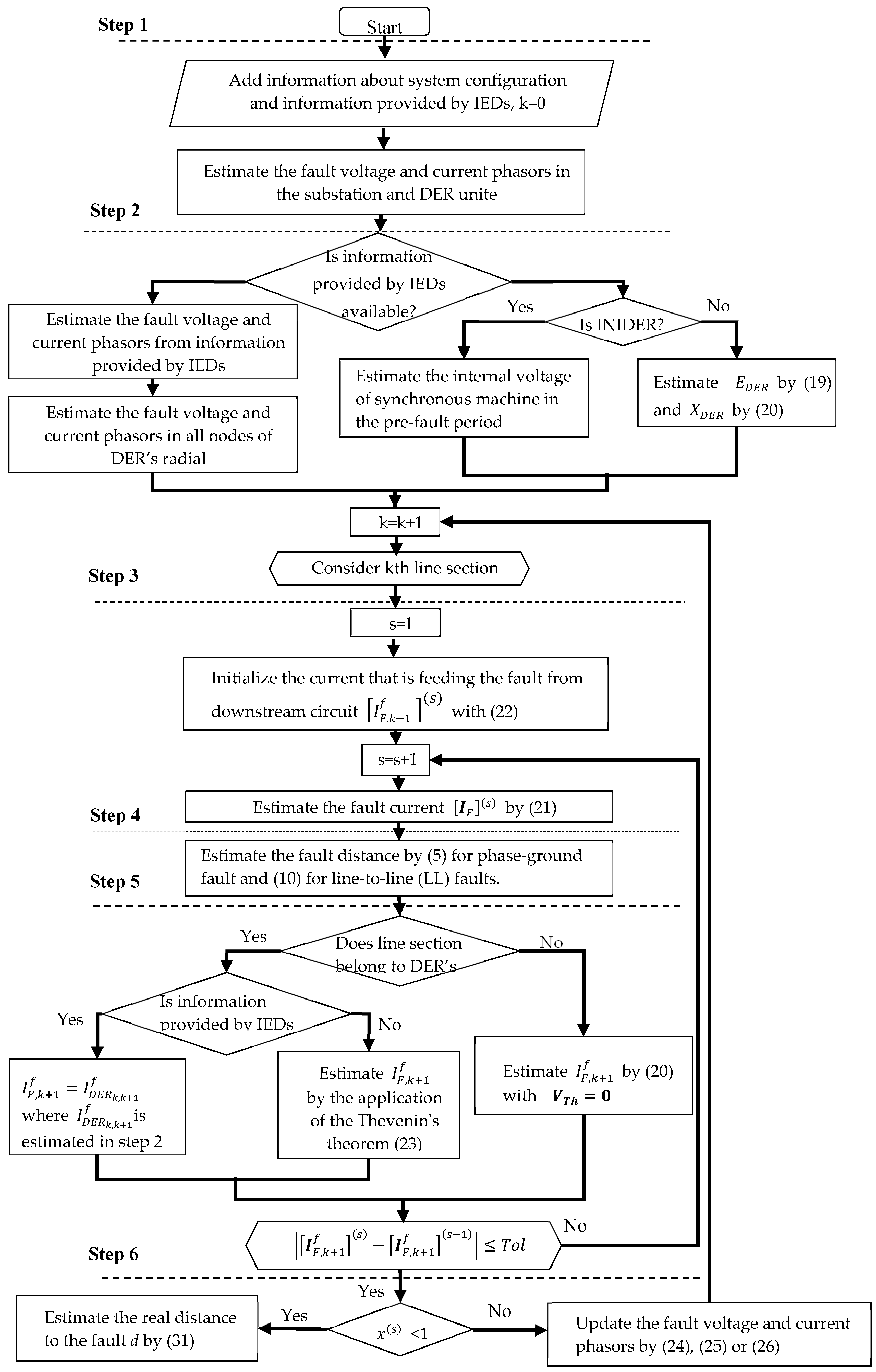
The proposed algorithm for fault location is capable to estimate the fault current with the DER’s available information. The generalized algorithm for estimating the fault distance is divided in 5 steps, as illustrated in Figure 3. The algorithm is explained in detail in the following.

3.1. Step 1: Processing Information of Power Distribution System and Substation Fault Records

In this step the information of the power distribution system is added, such as its topology and the electrical parameters of loads and distribution lines. Also, the substation fault voltage and current phasors are estimated by the application of the Fourier transform [3].

3.2. Step 2: Processing of DER Information

In this step the DER available information is processed, in order to consider its effect on the fault location algorithm. For the adaptive feature, the proposed method has two options: using DER electrical models or using the information provided by IEDs installed at the DER location. The algorithm was developed considering one DER. Nevertheless, multiple distributed generators can be considered by using the superposition and Thevenin’s theorem.

3.2.1. Using the Information Provided by IEDs Installed at the DER

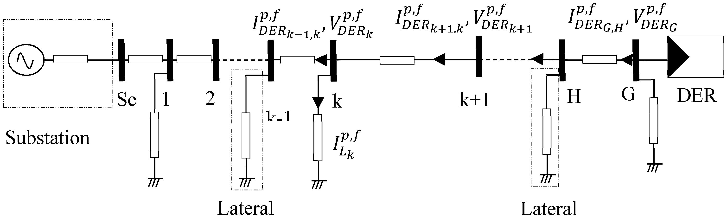
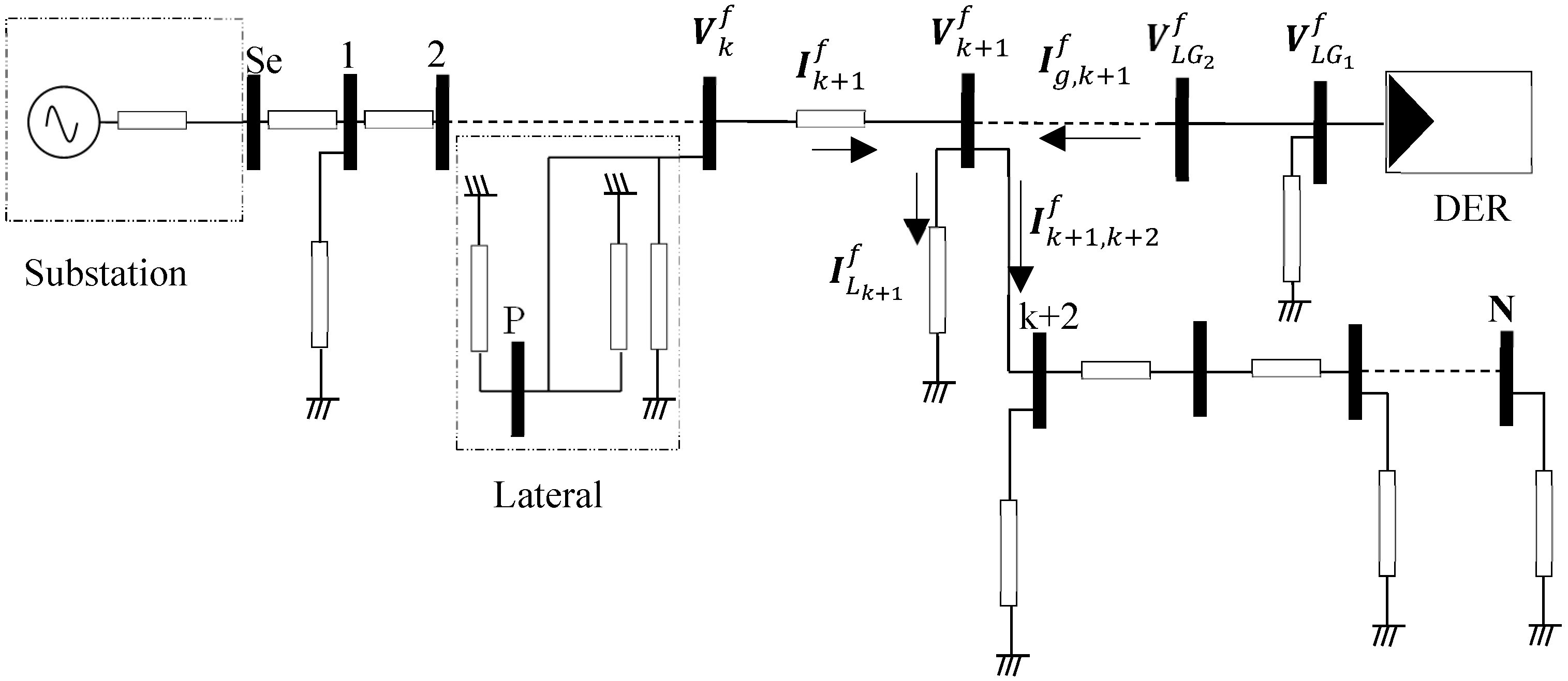
First, fault voltage and current phasors in DER are estimated. Then, the system parameters, line currents, and nodal voltages are estimated. Consider the power distribution system illustrated in Figure 4.

With the DER fault voltage and current phasors, a backward-sweep process from DER to substation can be performed, using Equations (11) and (12).

$$\left[\begin{array}{c}{\mathit{V}}_{DE{R}_k}^{p,f}\\ {\mathit{I}}_{DE{R}_k}^{p,f}\end{array}\right]=\left[\begin{array}{cc}{\mathit{d}}_l& -{\mathit{b}}_l\\ -{\mathit{c}}_l& {\mathit{a}}_l\end{array}\right]·\left[\begin{array}{c}{\mathit{V}}_{DE{R}_{k+1}}^{p,f}\\ {\mathit{I}}_{DE{R}_{k+1,k}}^{p,f}\end{array}\right]$$

(11)

$${\mathit{I}}_{DE{R}_{k-1,k}}^{p,f}={\mathit{I}}_{DE{R}_k}^{p,f}-{\mathit{I}}_{L_k}^{p,f}$$

(12)

where,

$${\mathit{a}}_l={\mathit{d}}_l=\mathit{I}+0,5·{\mathit{Z}}_{k,k+1}·{\mathit{Y}}_k$$

(13)

$${\mathit{b}}_l={\mathit{Z}}_{k,k+1}$$

(14)

$${\mathit{c}}_l={\mathit{Y}}_k+0.25·{\mathit{Y}}_k·{\mathit{Z}}_{k,k+1}·{\mathit{Y}}_k$$

(15)

Superscripts $\left(p\right)$ and $\left(f\right)$ indicate that prefault or fault period measurements are used. Moreover, for each line section under study between the substation and the DER illustrated in Figure 4, the current ${\mathit{I}}_{F,k+1}^f$ is assumed to be equal to ${\mathit{I}}_{DE{R}_{k-1,k}}^f$. This is in order to estimate the fault current, as it will be shown in step 3.

3.2.2. Using the Approximate Model of the Synchronous Machine for INIDER Model

If the DER parameters are known, the approximate model of the synchronous machine is used. This model is suitable for INIDER, given that their main element is a synchronous generator.

The main objective of this stage is to estimate the internal voltage of the synchronous generator model, using the prefault period substation voltage and current phasors (${\mathit{V}}_{Se}^p$ and ${\mathit{I}}_{Se}^p$). Therefore, considering Figure 5, a backward-sweep process from the substation to the DER node is implemented using Equations (16) and (17).

$$\left[\begin{array}{c}{\mathit{V}}_{k+1}^p\\ {\mathit{I}}_{k+1}^p\end{array}\right]=\left[\begin{array}{cc}{\mathit{d}}_l& -{\mathit{b}}_l\\ -{\mathit{c}}_l& {\mathit{a}}_l\end{array}\right]·\left[\begin{array}{c}{\mathit{V}}_k^p\\ {\mathit{I}}_{k,k+1}^p\end{array}\right]$$

(16)

$${\mathit{I}}_{k+1,k+2}^{p,f}={\mathit{I}}_{k+1}^p-{\mathit{I}}_{L_{k+1}}^p$$

(17)

In this process, the load is modeled as a constant impedance, which is appropriate in the subtransient fault period [31].

Once ${\mathit{V}}_G^p$ and ${\mathit{I}}_G^p$ are known, the synchronous machine internal voltage is estimated by Equation (18).

$$\mathit{E}={\mathit{V}}_G^p-{\mathit{Z}}_{DER}·{\mathit{I}}_G^p$$

(18)

This process eliminates the use of a load flow, as it is proposed previously [16,17,32]. Knowledge of the internal voltage in the DER model allows determining its behavior in the fault period, which allows the estimation of its current contribution to the fault point. The last is done by application of circuit reduction theorems such as Thevenin’s theorem, as it is presented in step 5 [16,32].

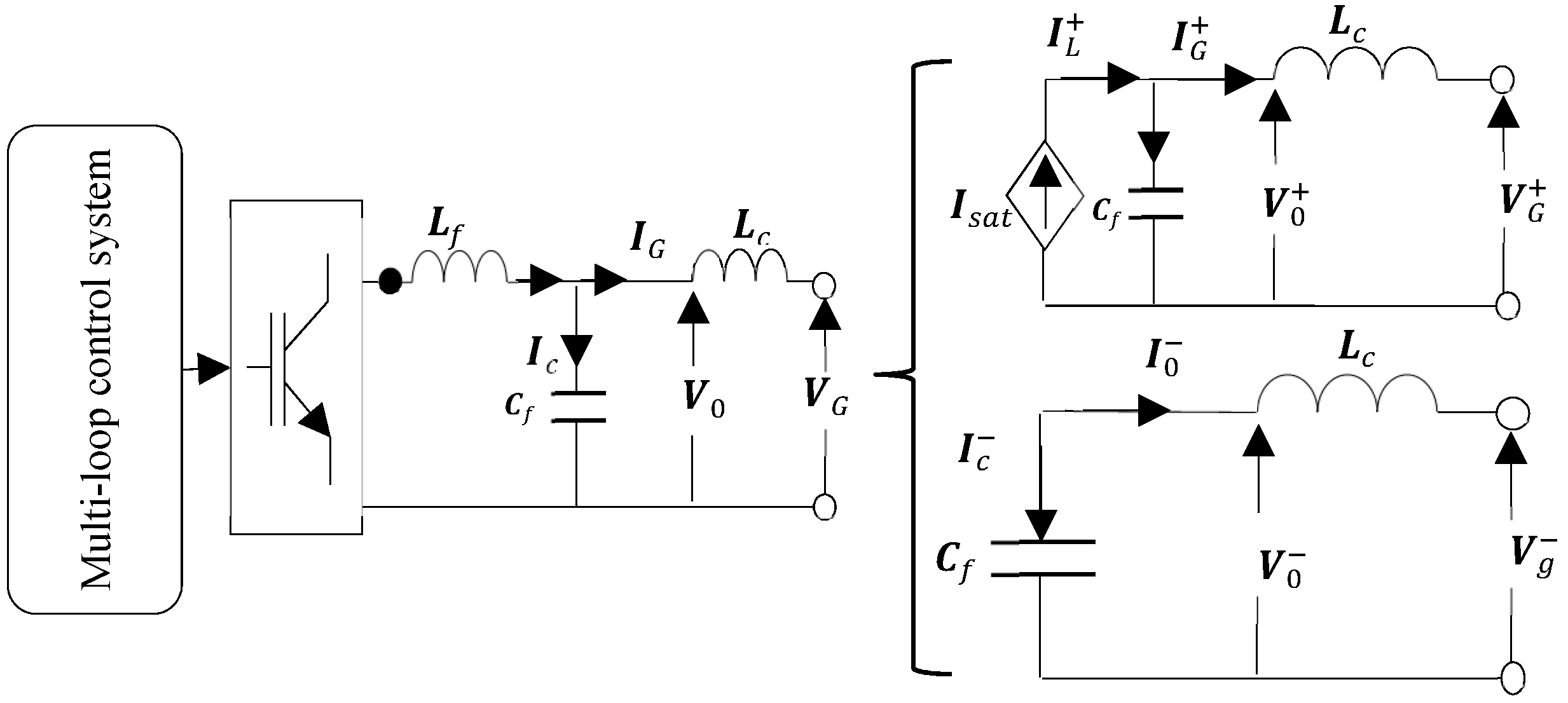
3.2.3. Using the IIDER Model in Current Limiting Mode

For IIDER, as for the inverter-based ones, the model will work well if the fault enables the DER to work on the current limiting mode. Thus, this study is focused on the model shown in Figure 6 as it is presented previously [27].

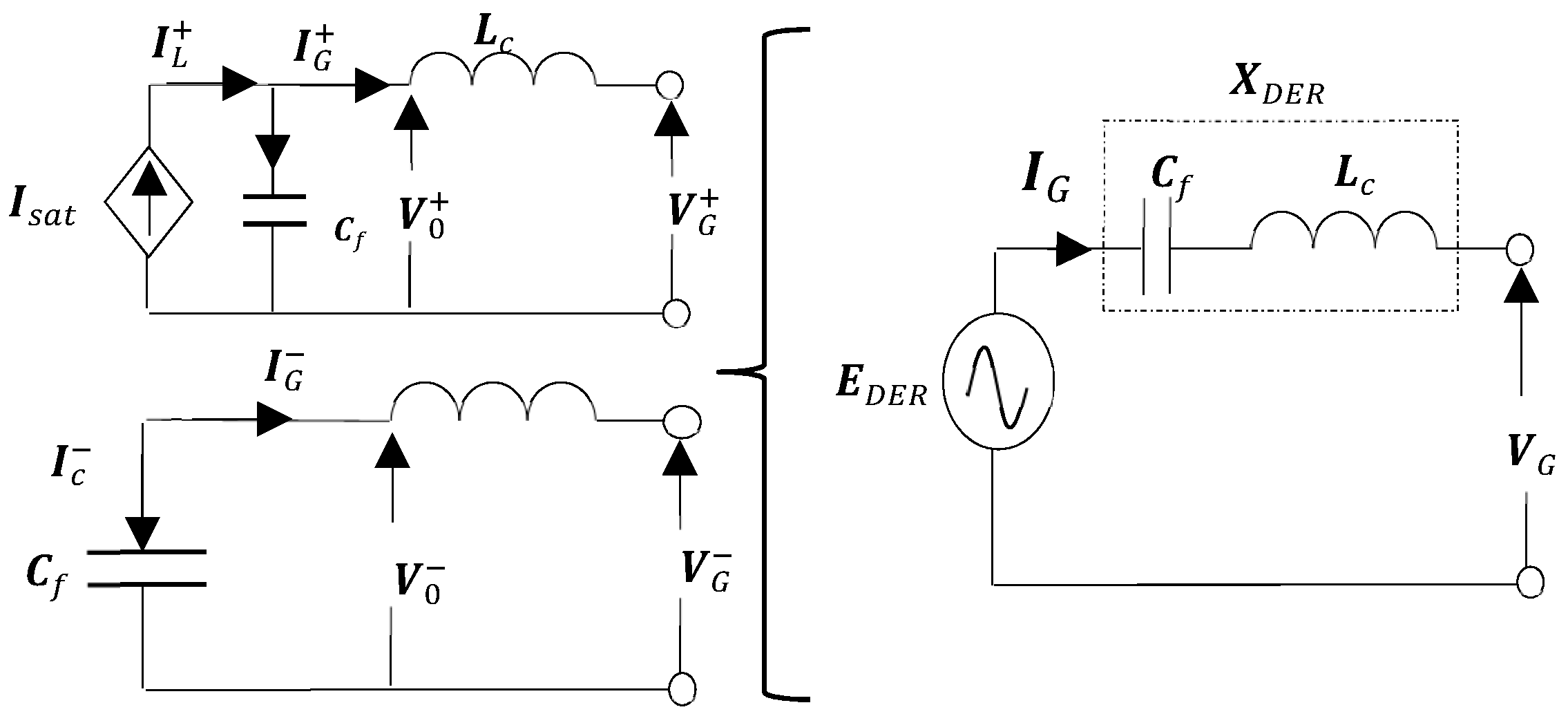
Making some algebraic manipulations, the circuit can be represented by a voltage source ${\mathit{E}}_{DER}$ and a reactance ${\mathit{X}}_{DER}$, which is a similar model to the synchronous generator model as shown in Figure 7.

Where, $E_{DER}$ and $X_{DER}$ are given by Equations (19) and (20).

$$E_{DER}=\frac{1}{j\omega C_f}·I_{sat}$$

(19)

$$X_{DER}=j\omega L_c+\frac{1}{j\omega C_f}$$

(20)

The previous analysis allows estimating the fault current contribution from DER to the fault point. The voltage $E_{DER}$ is known, since the saturation current $I_{sat}$ is typically twice the nominal current of the inverter. The inverter parameters are generally provided to the utilities when access to the distribution system is requested. However, if these parameters are not available, appropriate values may be obtained from technical catalogues by using the rated power and operating voltage of the inverter.

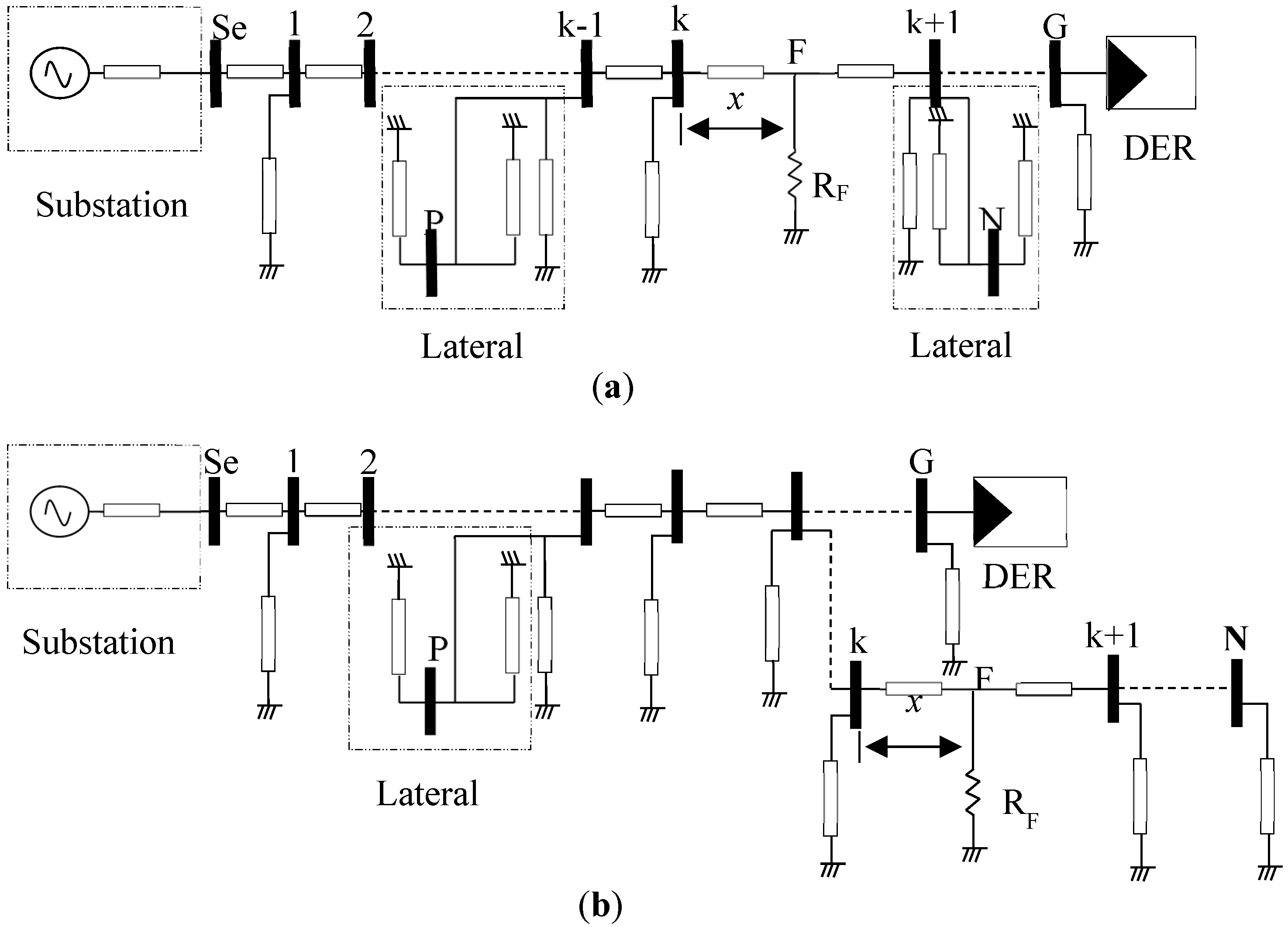
3.3. Step 3: Estimation of the Fault Current

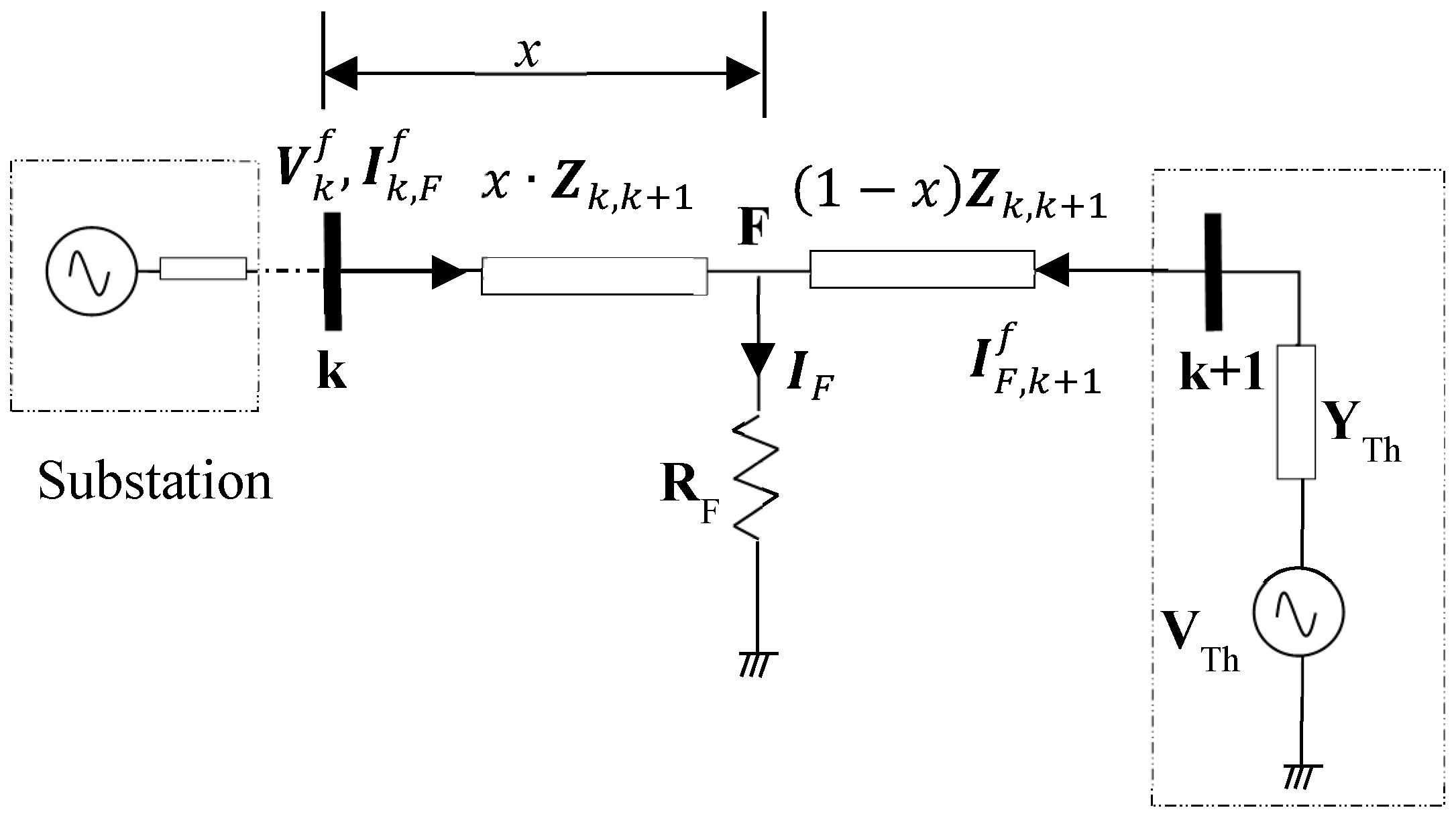
The estimation of the fault current depends on the location of the DER relative to the line section analyzed. The two possible conditions are illustrated in Figure 8.

A fault between the substation and the DER is represented in Figure 8a. In this case the DER effect is considered in the current feeding the fault from the downstream circuit. For this condition, the strategies of Section 3.5.1 and Section 3.5.2 are used. For the second condition, the DER effect is considered in the current feeding the fault from the upstream circuit. Therefore, the fault current is estimated on the basis of the fault distance $x$; as in the original formulation proposed previously [11]. Therefore, the fault current is given by Equation (21).

$${\mathit{I}}_F={\mathit{I}}_{k,F}^f+{\mathit{I}}_{F,k+1}^f$$

(21)

Given that the fault current is a function of $x$, it is necessary to perform an iterative process to determine a precise value for the current ${\mathit{I}}_{F,k+1}^f$, as shown in Figure 3. The initial value adopted for ${\mathit{I}}_{F,k+1}^f$ is given by Equation (22).

$${\mathit{I}}_{F,k+1}^f={\mathit{I}}_{k,F}^p$$

(22)

3.4. Step 4: Estimation of the Fault Location for Each Section

Given the fault current, the fault distance in each section is calculated by means of Equation (5) if it is from a ground-phase fault, or by means of Equation (10) if it is from a line-line fault, as presented previously.

3.5. Step 5: Iterative Process to Determine the Fault Current

The iterative process to determine the fault current can be carried out in two different ways: by using the information provided by IEDs or by using the DER electrical model.

3.5.1. Estimation of the Fault Current by Using the Information Provided by IEDs

When the information provided by IEDs is available, the estimation of the fault current is straightforward. For this case, the current feeding the fault from the downstream circuit ${\mathit{I}}_{F,k+1}^f$ is assumed to be ${\mathit{I}}_{F,k+1}^f={\mathit{I}}_{DE{R}_{k-1,k}}^f$, where ${\mathit{I}}_{DE{R}_{k-1,k}}^f$ is the current estimated in step 2.

3.5.2. Estimation of the Fault Current by Using the DER Model

When the information provided by the IEDs is not available, the DER model is used. In this case, the DER contribution current to the fault point is calculated by the application of Thevenin’s theorem.

Considering the power distribution system illustrated in Figure 8a, it is reduced to the circuit shown by Figure 9.

The Thevenin’s voltage is estimated from the internal voltage vector of the synchronous generator calculated in the step 2 for INIDER, or from the current saturation and DER filter parameters for IIDER. The Thevenin’s admittance matrix is estimated by short-circuiting the internal generator voltage, and calculating the equivalent admittance of the system downstream from the DER to node k + 1. ${\mathit{I}}_{F,k+1}^f$ is estimated from the fault voltage vector ${\mathit{V}}_F$, the Thevenin voltage vector ${\mathit{V}}_{Th}$, and the Thevenin’s admittance matrix ${\mathit{Y}}_{Th}$, as shown by Equation (23).

$${\mathit{I}}_{F,k+1}^f={\mathit{Y}}_{Th}·{\left[\left(1-x\right)·{\mathit{Z}}_{k,k+1}·{\mathit{Y}}_{Th}+\mathit{I}\right]}^{-1}·\left({\mathit{V}}_F-{\mathit{V}}_{Th}\right)$$

(23)

Voltage and current vectors are estimated from the circuit parameters, current, and voltage measurements at the substation. Therefore, the fault current is given by the same Equation (21).

3.6. Step 6: Update the Voltage and Current Vectors, and Distance from the Substation Up to the Fault Point

In this step, one of the following two actions are taken: the update of the voltage and current vectors, or the calculation of the distance from the fault point. If the first action is taken, the algorithm goes back to step 3 and continues with a new line section. On the other hand, if the second action is taken, the algorithm determines the fault distance and finishes. The two actions are detailed to continue:

3.6.1. Update the Voltage and Current Vectors

As shown in the algorithm presented in Figure 3, the fault is estimated downstream of the first system section and then, the values of voltage and current measured at the local terminal are updated to the next system buses by Equations (24) and (25).

$$\left[\begin{array}{c}{\mathit{V}}_{k+1}^{p,f}\\ {\mathit{I}}_{k+1}^{p,f}\end{array}\right]=\left[\begin{array}{cc}{\mathit{d}}_l& -{\mathit{b}}_l\\ -{\mathit{c}}_l& {\mathit{a}}_l\end{array}\right]·\left[\begin{array}{c}{\mathit{V}}_k^{p,f}\\ {\mathit{I}}_{k,k+1}^{p,f}\end{array}\right]$$

(24)

$${\mathit{I}}_{k+1,k+2}^{p,f}={\mathit{I}}_{k+1}^{p,f}-{\mathit{I}}_{L_{k+1}}^{p,f}$$

(25)

Equation (25) is used for all system nodes, except for the node where the lateral of the DER is connected. For this node, the current ${\mathit{I}}_{\mathit{k}+1,\mathit{k}+2}^{\mathit{p},\mathit{f}}$ is updated by Equation (26).

$${\mathit{I}}_{k+1,k+2}^{p,f}={\mathit{I}}_{k+1}^{p,f}-{\mathit{I}}_{L_{k+1}}^{p,f}+{\mathit{I}}_{g,k+1}^{p,f}$$

(26)

where ${\mathit{I}}_{g,k+1}^{p,f}$ is the current contribution from the DER to the node $k+1$, as shown in Figure 10.

The proposed fault location algorithm considers that the DER can be allocated in any node of the system. Therefore, the current contribution from the DER to the node $k+1$ is calculated from the nodal admittance matrix of the lateral of the DER, as shown by Equations (27) and (28).

$$\left[\begin{array}{c}\begin{array}{c}{\mathit{V}}_{L{G}_1}^f\\ {\mathit{V}}_{L{G}_2}^f\\ {\mathit{V}}_{L{G}_3}^f\end{array}\\ \begin{array}{c}⋮\\ ⋮\\ {\mathit{V}}_{L{G}_k}^f\end{array}\end{array}\right]={\left[\begin{array}{cccccc}{\mathit{Y}}_{l{g}_{11}}& {\mathit{Y}}_{l{g}_{12}}& 0& 0& \cdots & 0\\ {\mathit{Y}}_{l{g}_{21}}& {\mathit{Y}}_{l{g}_{21}}& {\mathit{Y}}_{l{g}_{23}}& 0& \cdots & 0\\ 0& {\mathit{Y}}_{l{g}_{32}}& {\mathit{Y}}_{l{g}_{33}}& {\mathit{Y}}_{l{g}_{23}}& \cdots & 0\\ 0& 0& 0& \ddots & \cdots & 0\\ ⋮& ⋮& ⋮& ⋮& \ddots & ⋮\\ 0& 0& 0& 0& {\mathit{Y}}_{l{g}_{k,k-1}}& {\mathit{Y}}_{l{g}_{k,k}}\end{array}\right]}^{-1}·\left[\begin{array}{c}\begin{array}{c}{\mathit{y}}_{DER}·\mathit{E}\\ 0\\ 0\end{array}\\ \begin{array}{c}⋮\\ ⋮\\ {\mathit{y}}_{l{g}_{k,k+1}}·{\mathit{V}}_{k+1}^f\end{array}\end{array}\right]$$

(27)

$${\mathit{I}}_{g,k+1}^f={\mathit{y}}_{l{g}_{k,k+1}}·\left({\mathit{V}}_{L{G}_k}^f-{\mathit{V}}_{k+1}^f\right)$$

(28)

with,

$${\mathbf{Y}}_{{\lg }_{\mathrm{ii}}}={\displaystyle \sum _{\mathrm{j}\Omega \mathrm{i}}^{\mathrm{k}}}{\mathbf{y}}_{{\lg }_{\mathrm{ij}}}$$

(29)

$${\mathbf{Y}}_{{\lg }_{\mathrm{ij}}}=-{\mathbf{y}}_{{\lg }_{\mathrm{ij}}}$$

(30)

3.6.2. Calculation of Distance from the Substation to the Fault Point

After estimating the fault point, distance $d$ from the substation to the fault point is also estimated. This is made by means of Equation (31),

$$d={\displaystyle \sum _{i=1}^{nt-1}}{L}_i+x·L_{nt}$$

(31)

4. Case Studies

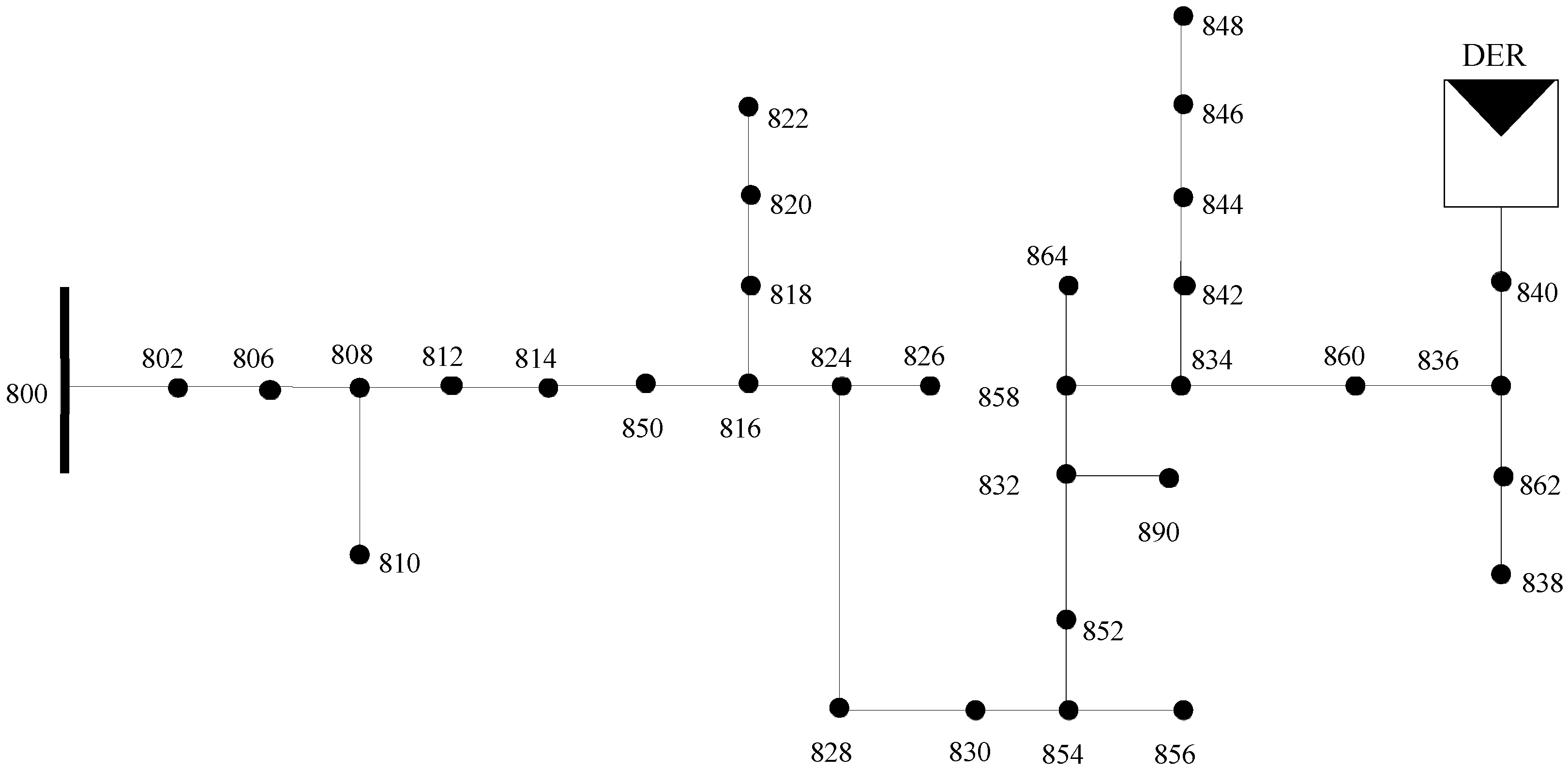
The proposed method was validated with a modified IEEE 34-node test feeder [33]. This feeder is located in the state of Arizona (USA) and operates at a voltage of 24.9 kV. Figure 11 presents the IEEE 34-node test feeder.

The relevant characteristics of the test feeder are the presence of single, two-phase, and three-phase laterals, multiple wire sizes, and unbalanced loads of concentrated and distributed nature. This system is simulated with the software EMTP-ATP, and modified by inserting a DER. This test feeder has been widely used for fault location studies in distribution networks [13,20,21,22,23]. Two considerations for validation of the algorithms are made. The first consideration is to assume that IEDs have been installed in the substation and the DER location. It is also assumed that the information gathered is sufficient to determine the voltage and current phasors during the prefault and fault periods. The second consideration assumes that there is no available information collected by IEDs at the DER location; therefore, the electrical model of the DER is used. Under these conditions, the method is validated by considering three scenarios:

Scenario 1: This scenario considers only the influence of the fault resistance and the fault type.

Table 1. Simulation data for scenario 1. DER: distributed energy resources; IED: intelligent electronic devices.

Parameters	Information Available of IEDs	Factors	Located Faults
DER penetration level: 10%	Yes	Faults resistance between: 0–100 Ω in steps of 5 Ω	5481
Load condition: Nominal	NO DER type: INIDER	Fault types: A-g, B-g, C-g, AB, BC, CA, AB-g, BC-g, CA-g, ABC, and ABC-g	5481
	Total faults		10,862

presents the description for this scenario.

Scenario 2: This scenario considers only the influence of the load. Three ranges of nominal load are considered, according to the information given in

Table 2. Simulation data for scenario 2.

Parameters	Information Available of IEDs	Factors	Located Faults
DER penetration level: 10%	Yes	Random load variation: 30–60%, 60–100%, 100–140%	129
Fault resistance: 10 Ω.	NO DER type: INIDER		129
Fault type: Three phase faults	NO DER type: IIDER		129
	Total faults		987

. For each of these ranges, a uniformly distributed value is used as the system load.

Scenario 3: This scenario considers only the influence of the DER penetration level. Three different values of penetration level are considered in

Table 3. Simulation data for scenario 3.

Parameters	Information Available of IEDs	Factors	Located Faults
Load condition: Nominal Fault resistance: 10 Ω. Fault type: Three phase faults	Yes	DER penetration level: 10%, 20%, 30%	129
	NO DER type: INIDER		129
	NO DER type: IIDER		129
	Total faults		987

.

5. Results and Analysis

The results obtained with the proposed method are given in terms of a percentage error, which is calculated by means of Equation (32).

$$\%\mathrm{Error}=\frac{{\mathrm{d}}_{\mathrm{real}}-{\mathrm{d}}_{\mathrm{estimated}}}{{\mathrm{d}}_{\mathrm{total}}}·100\%$$

(32)

In the following, the results are analyzed for each simulated scenario.

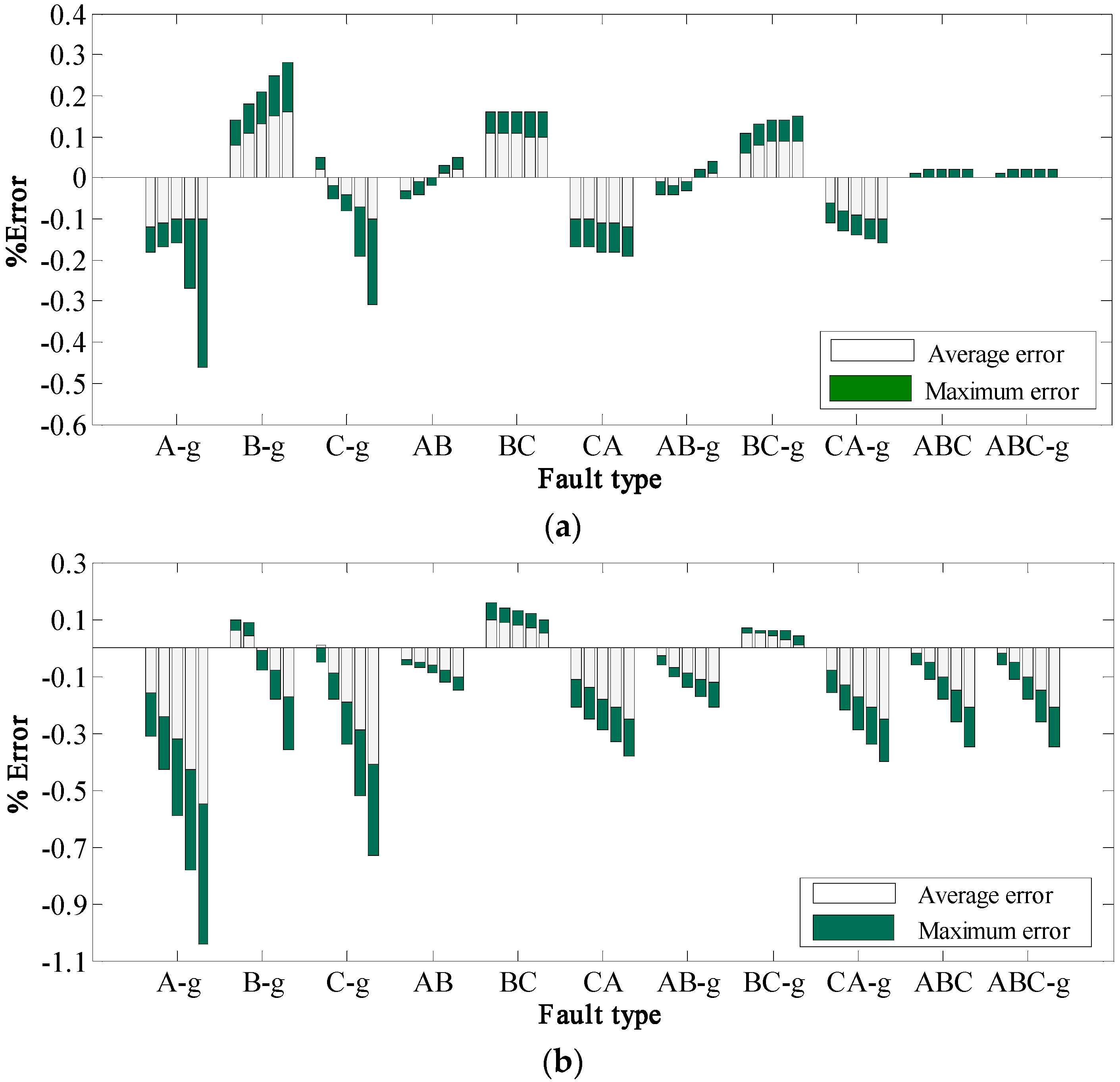
5.1. Scenario 1: Fault Resistance Effect

The FL errors are classified for each fault type. At the same time, the errors of each fault type are presented in five different ranges of fault resistance with 20 Ω intervals. Average and maximum errors are also identified in Figure 12a,b.

The results obtained using the information of IEDs show a maximum average error of 0.16% and a maximum error of −0.46%. It is worth noticing here that both errors occurred for the single-phase to ground fault. These errors correspond to 90 m and 270 m, considering a feeder with 58 km of length. On the other hand, when the DER electrical model is used, the method’s performance decreases, obtaining a maximum average error of 0.55% and a maximum error of 1.04%. These errors were also obtained for the single-phase to ground fault. As expected, the lowest location errors are found with the model that uses the information of the IEDs.

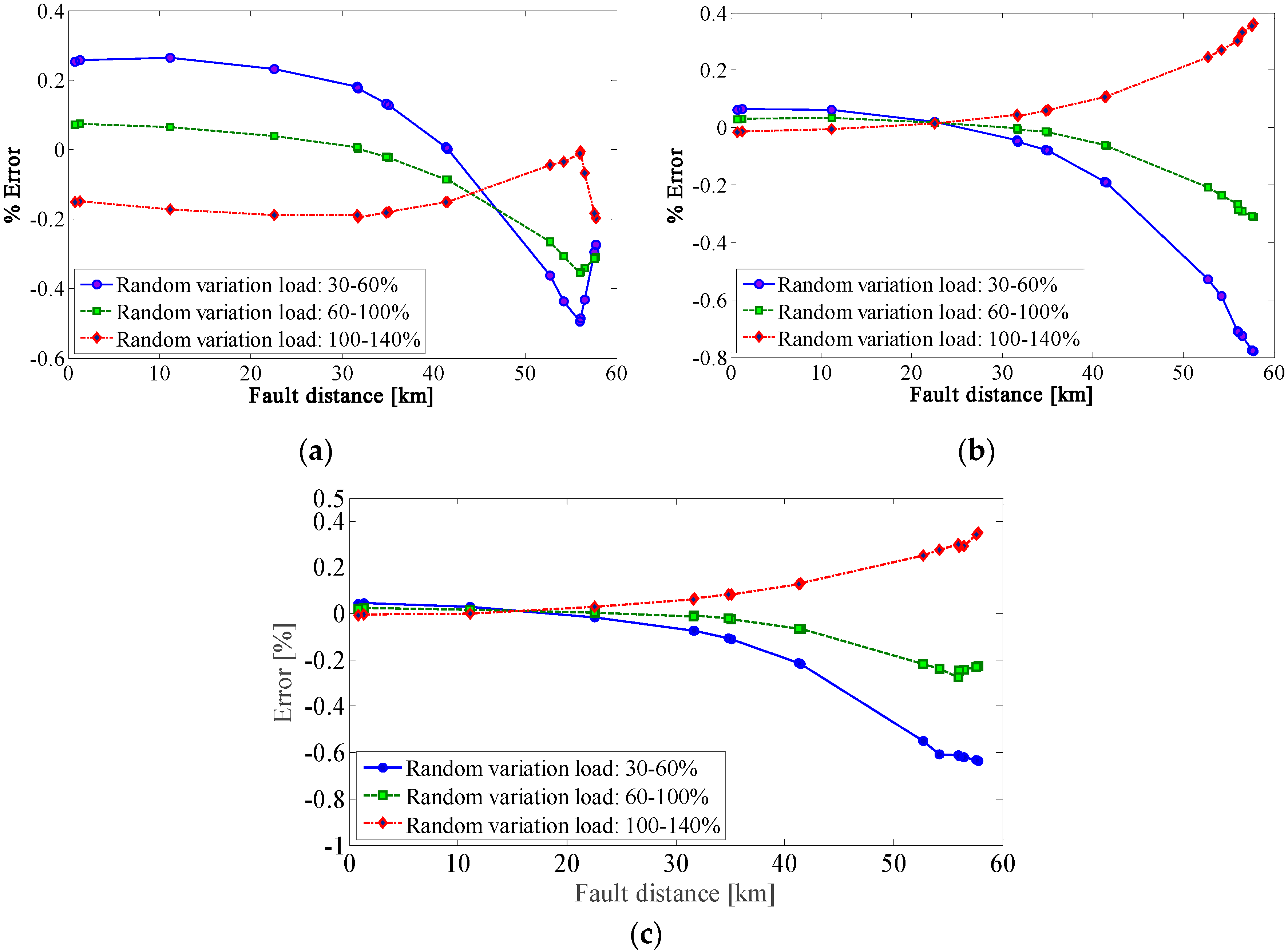
5.2. Scenario 2: Load Variation Effect

The results for this scenario are presented in Figure 13, which shows the estimated error of the fault distance calculated by Equation (32), and the actual distance to the fault.

For this scenario, a small difference of the method’s performance is observed, especially from the substation to the middle of the feeder. When IEDs information is used, the method presents a performance with errors below 0.2%. However, when IEDs information is not available, the proposed method presents a better performance. The errors are below 0.05% for both models of DER (INIDER and IIDER). On the contrary, for faults located after 30 kms, and using IED information, the method presented better performance than using the DER model. However, the maximum error for these cases is of about 0.8%. Additionally, the test results show a small correlation between the method’s performance and the load value. This behavior occurs because in this work, no load compensation strategy was implemented. Nevertheless, a compensation strategy can be used as proposed previously [34].

For the nominal-high load condition, the behavior of the method is of subestimation. In other words, the method tends to estimate a distance lower than the real distance to the fault. In contrast, for scenarios where the load decreases, the method tends to overestimate the distance to the fault. This is explained because as the load increases, the method observes a lower impedance of the system and estimates a lower distance to the fault. Nevertheless, test results show very low error values. This is because the use of Thevenin models, decreases the impact of individual model parameter errors.

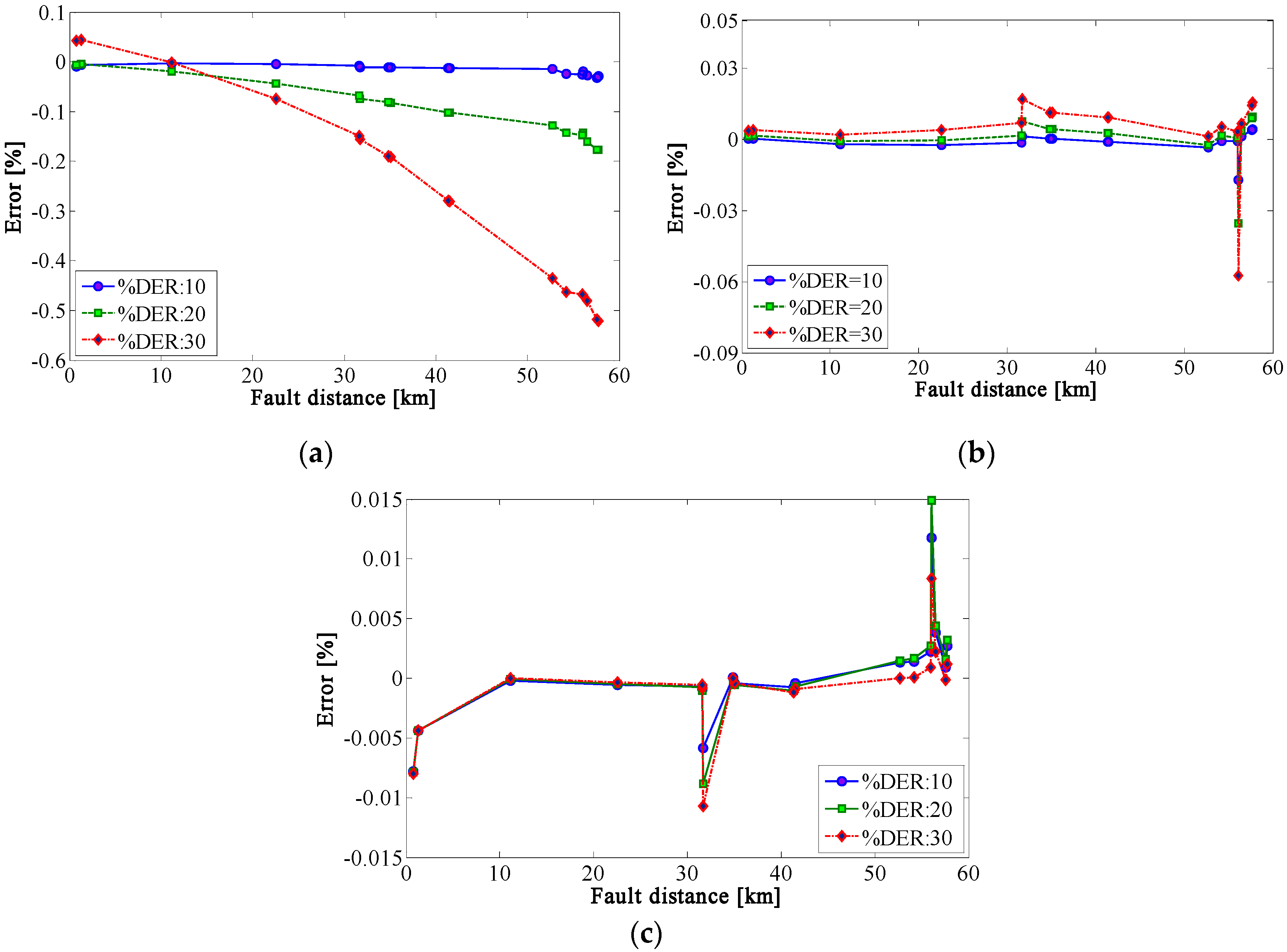
5.3. Scenario 3: DER Penetration Level Effect

Figure 14a–c presents the performance for the proposed method using the IEDs information and using the DER electrical model.

For this scenario, a clear difference is observed in the performance of the method. When IEDs information is used, the method exhibits an excellent performance with errors below 0.02% (approximately 10 m in a feeder with 58 km of length). Also, its performance is quasi-invariant for different DER penetration levels. When the DER electrical model for INIDER is used, the performance of the method decreases significantly in relation to the performance obtained with IEDs information. For this case, a clear tendency to overestimate the fault distance as DER penetration level increases are observed; reaching an error of 0.5% for a penetration level of 30%. This behavior is due to the increasing penetration, which increases the error in the estimation of the current supplied to the fault point from the DER. On the other hand, the method presents errors lower than 0.06% when using the DER electrical model for IIDER. A tendency to underestimate the fault distance when the DER penetration level increases, is observed. However, its performance is better than when the INIDER model is used. This occurs because the contribution of the current from the IIDER to the fault point is lower than in the case of the INIDER, and this current is estimated by an iterative process.

5.4. Comparison Test

Two state-of-the-art methods were implemented and compared with the proposed analytical methodology: Nunes et al.’s method [16,17] and Bedoya et al.’s method [21]. These methods were validated and compared using scenario 1.

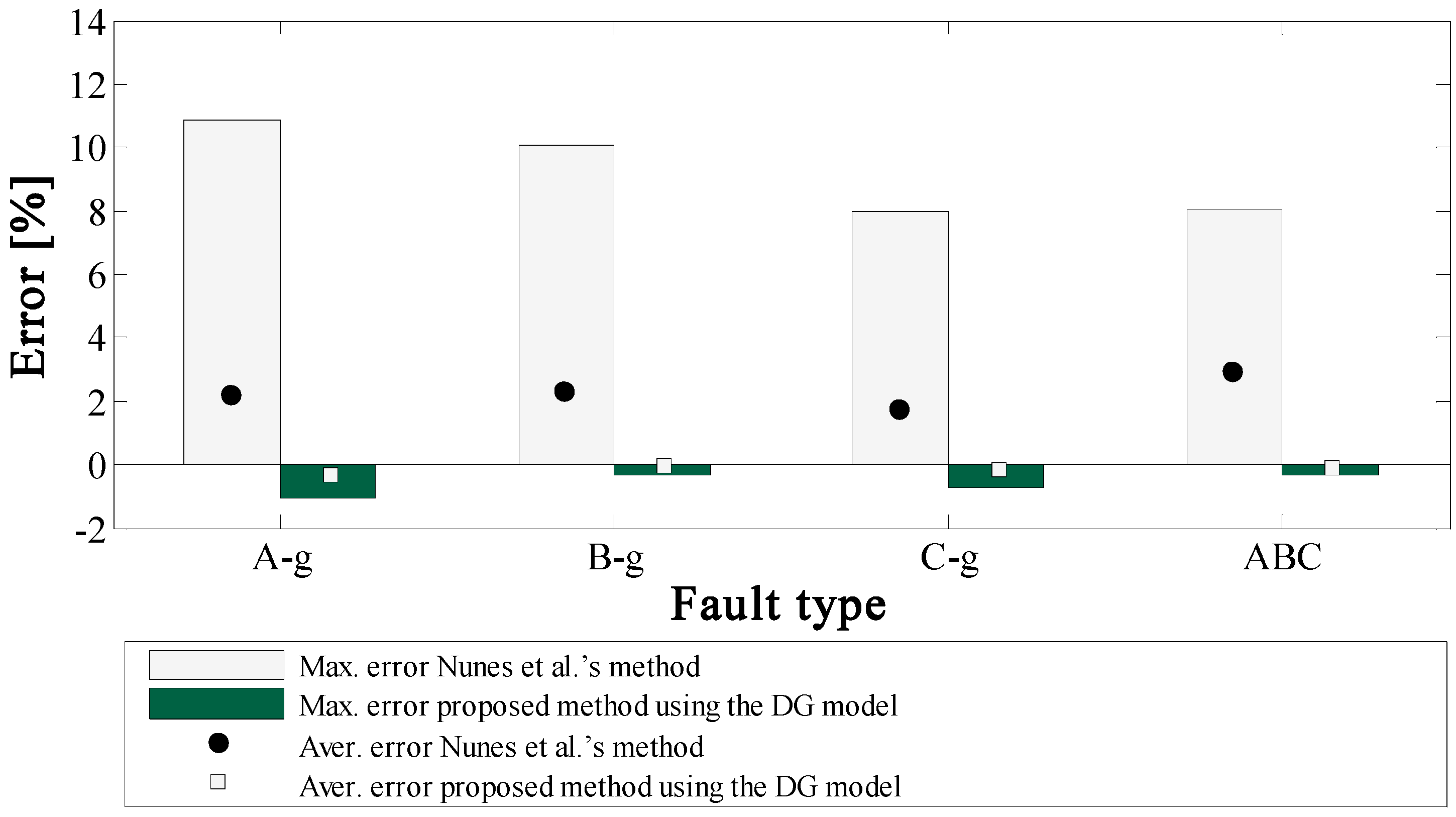
The method proposed by Nunes et al. uses the synchronous machine model to consider the DG effect on the fault location. Therefore, it was compared with the method of this paper, using also the INIDER electrical model. Because of the large number of results, they are presented in a bar graph using the average and maximum errors obtained for each fault type, as shown in Figure 15.

The test results show the better accuracy of our method when compared with the method proposed by Nunes et al. Nunes et al.’s method presents errors of up to 11% and an average error of 2% for faults with fault resistances between 0 and 100 ohms. While for our method, the errors in estimating the fault distance are lower than 1.1%, and the average error is 0.6%. This difference in accuracy between both methods is caused mainly because of the capacitive effect, which is not considered in the formulation of Nunes et al.

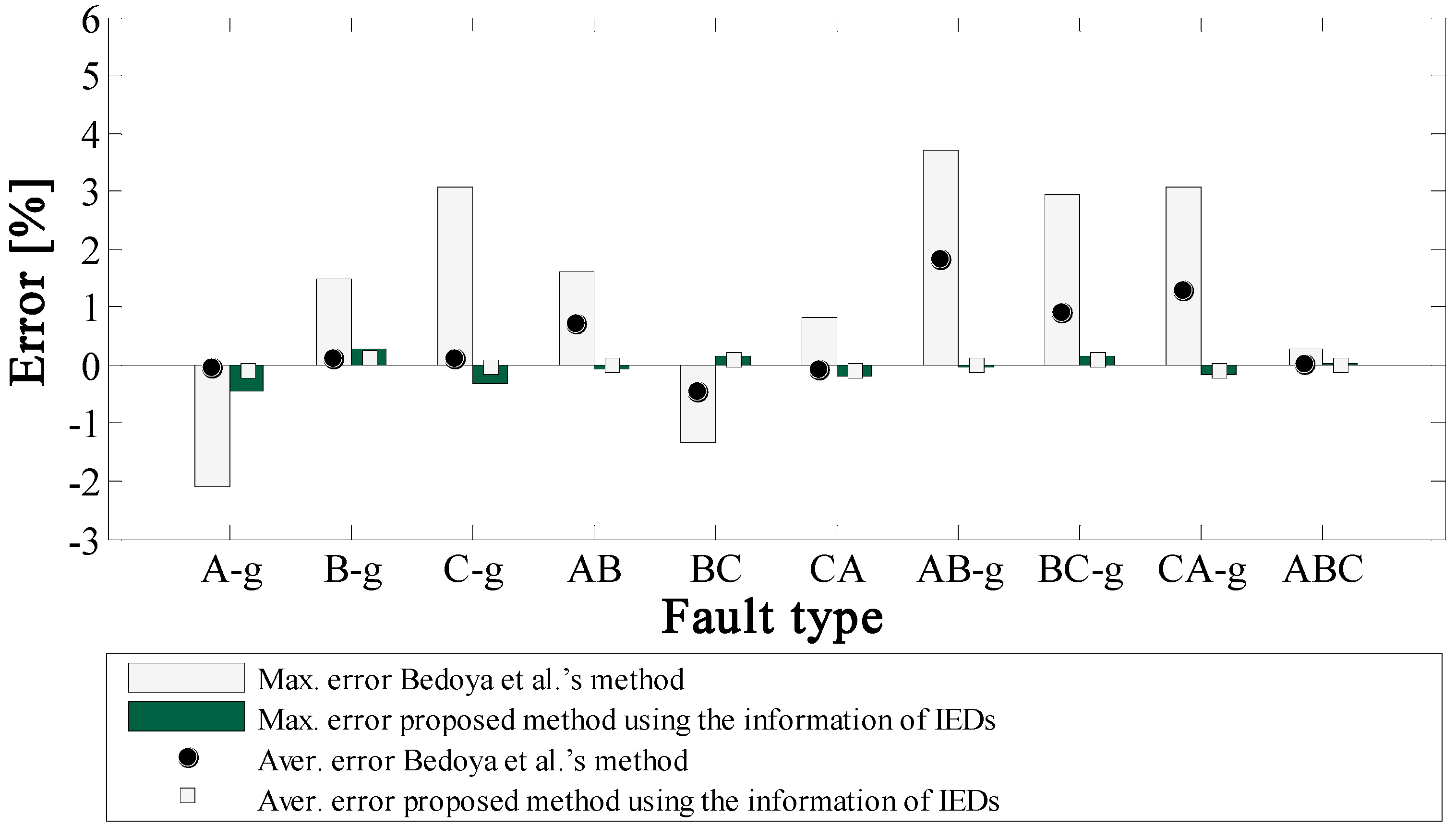
Similarly, the method proposed by Bedoya et al. was compared with our method. For this comparative test, our method used information from the IED located at the DER, since the Bedoya et al.’s method uses synchronized measurements at the DER terminal. Figure 16 presents the results obtained for Bedoya et al.’s method and our method.

The results obtained show the better accuracy of our method when compared with the method proposed by Bedoya et al. This better accuracy is observed in the maximum errors obtained for each fault type. Nonetheless, for some fault types (A-g, B-g, C-g, C-A, and ABC) the average errors are very low and are comparable to those obtained with the method of this paper.

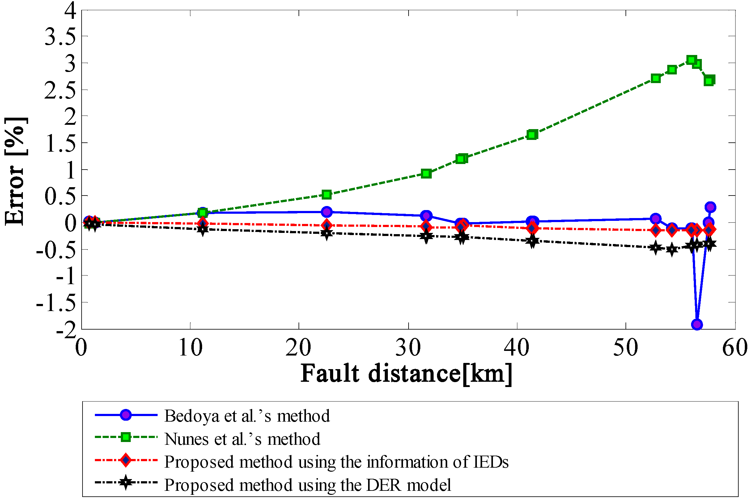
Figure 17 compares two state-of-the-art methods with the one proposed in this paper; the last one considering IED information, or the DER electrical model. This comparison is made for one case of the scenarios evaluated in the comparison tests. The figure allows to understand why the Nunes method presents a low performance: it depends on the fault resistance and the location of the fault. The figure also shows that the performance of the method proposed in this paper, using the DER electrical model, is comparable with the performance of Bedoya et al.’s method. This is relevant because it shows the robustness of our method, even when the IED information is not available.

6. Discussion

The fault location method proposed in this paper showed to be robust for the validation scenarios. The effect of the fault resistance, random variation of the load, level of penetration of dispersed generation sources, and the location of the fault, were analyzed.

The performance of the method is adequate, with errors lower than 1.1%. The factor that produces the highest error is the fault resistance. This effect is significantly intensified with the type of fault; the single-phase faults the ones that affect the location accuracy the most. This is expected, since being shown previously [35], with the increase of the fault resistance, the impedance seen by the impedance-based fault location methods tends to be greater than the real impedance of the power system.

However, the factor that produces a greater location error is the DER penetration level: the greater the DER penetration level, the greater the error. However, the error decreases if the IED information is available. Nevertheless, when IED information is not available, the DER electrical model is used, and an iterative process is made to determine the DER contribution to the fault current. This process is less accurate than using the current measured by the IEDs in the DER and the accuracy is affected by the location of the fault.

On the other hand, the load variation also showed an effect on the performance of the proposed method. This is expected for two reasons: first, the proposed method is as impedance-based method; therefore, any variation in the load will affect the impedance of the power system. The second reason is that the power system impedance variation due to the load variation must be compensated in the fault location formulation. If a compensation strategy is not used, a significant error on the estimation of the fault distance will be introduced. For the proposed method, a compensation strategy was not used, which produces an increase in the error with a behavior depending on the load variation features.

7. Conclusions

This work presented an adaptive impedance-based fault location algorithm for active distribution systems. This method showed to be robust and adaptive, obtaining estimation errors lower than 1.1% with or without available information provided by IEDs.

The proposed method showed a satisfactory performance under the effect of different features and fault situations. In the case of the fault resistance effect, the method presented a small increase in the estimation error, which could be increased by the faulted phases’ loading and the fault incidence angle. However, this increase is acceptable. The load variation effect shows that when load decreases relative to its nominal value, the proposed method tends to overestimate the fault distance. On the other hand, when the load increases relative to its nominal value, the method tends to underestimate the fault distance. This is justified because as the load increases, the method sees a lower impedance from the substation to the fault point and therefore, estimates a lower fault distance and vice versa.

The effect of the DER penetration level was very small when the IEDs information was used. However, when this information was not available, an increase in the estimated error of the fault distance was observed and showed to be directly proportional to the DER penetration level. This error is caused by the model used for the DER, since it corresponds to an approximate model; the impedance-based fault location methods are very sensitive to the correct estimation of the fault current. However, this increase was not significant, presenting errors lower than 1.1% on the estimation of the fault distance.

Finally, the proposed method performance was compared with two state-of-the-art methods, showing outstanding performance.

References

- Reddy, M.J.; Rajesh, D.V.; Gopakumar, P.; Mohanta, D.K. Smart Fault Location for Smart Grid Operation Using RTUs and Computational Intelligence Techniques. IEEE Syst. J. 2014, 8, 1260–1271. [Google Scholar] [CrossRef]
- Napis, N.F.; Abd Kadir, A.F.; Khatib, T.; Hassan, E.E.; Sulaima, M.F. An Improved Method for Reconfiguring and Optimizing Electrical Active Distribution Network Using Evolutionary Particle Swarm Optimization. Appl. Sci. 2018, 8, 804. [Google Scholar] [CrossRef]
- Saha, M.M.; Izykowski, J.; Rosolowski, E. Fault Location on Power Networks; Springer: Berlin, Germany, 2010. [Google Scholar]
- Pavlatos, C.; Vita, V.; Dimopoulos, A.C.; Ekonomou, L. Transmission lines’ fault detection using syntactic pattern recognition. Energy Syst. 2018. [Google Scholar] [CrossRef]
- Liang, R.; Fu, G.; Zhu, X.; Xue, X. Fault location based on single terminal travelling wave analysis in radial distribution network. Int. J. Electr. Power Energy Syst. 2015, 66, 160–165. [Google Scholar] [CrossRef]
- Ye, L.; You, D.; Yin, X.; Wang, K.; Wu, J. An improved fault-location method for distribution system using wavelets and support vector regression. Int. J. Electr. Power Energy Syst. 2014, 55, 467–472. [Google Scholar] [CrossRef]
- Rafinia, A.; Moshtagh, J. A new approach to fault location in three-phase underground distribution system using combination of wavelet analysis with ANN and FLS. Int. J. Electr. Power Energy Syst. 2014, 55, 261–274. [Google Scholar] [CrossRef]
- Pavlatos, C.; Vita, V. Linguistic Representation of Power System Signals. In Electricity Distribution: Intelligent Solutions for Electricity Transmission and Distribution Networks; Springer: Berlin/Heidelberg, Germany, 2016; pp. 285–295. [Google Scholar]
- Xiu, W.; Liao, Y. Novel fault location methods for ungrounded radial distribution systems using measurements at substation. Electr. Power Syst. Res. 2014, 106, 95–100. [Google Scholar] [CrossRef]
- Gabr, M.A.; Ibrahim, D.K.; Ahmed, E.S.; Gilany, M.I. A new impedance-based fault location scheme for overhead unbalanced radial distribution networks. Electr. Power Syst. Res. 2017, 142, 153–162. [Google Scholar] [CrossRef]
- Salim, R.H.; Salim, K.C.; Bretas, A.S. Further improvements on impedance-based fault location for power distribution systems. IET Gener. Transm. Distrib. 2011, 5, 467–476. [Google Scholar] [CrossRef]
- Dashti, R.; Salehizadeh, S.M.; Shaker, H.R.; Tahavori, M. Fault Location in Double Circuit Medium Power Distribution Networks Using an Impedance-Based Method. Appl. Sci. 2018, 8, 1034. [Google Scholar] [CrossRef]
- Adewole, A.C.; Tzoneva, R. Distribution network fault detection and diagnosis using wavelet energy spectrum entropy and neural networks. Int. Rev. Electr. Eng. 2014, 9, 165–173. [Google Scholar]
- Gazzana, D.S.; Ferreira, G.D.; Bretas, A.S.; Bettiol, A.L.; Carniato, A.; Passos, L.F.; Silva, J.E. An integrated technique for fault location and section identification in distribution systems. Electr. Power Syst. Res. 2014, 115, 65–73. [Google Scholar] [CrossRef]
- Akorede, M.F.; Hizam, H.; Pouresmaeil, E. Distributed energy resources and benefits to the environment. Renew. Sustain. Energy Rev. 2010, 14, 724–734. [Google Scholar] [CrossRef] [Green Version]
- Nunes, J.U.N.; Bretas, A.S. Impedance-based fault location formulation for unbalanced primary distribution systems with distributed generation. In Proceedings of the 2010 International Conference on Power System Technology, Hangzhou, China, 24–28 October 2010; pp. 1–6. [Google Scholar]
- Nunes, J.U.N.; Bretas, A.S. An extended fault location formulation for unbalanced distribution feeders with distributed generation. In Proceedings of the 2010 Modern Electric Power Systems, Wroclaw, Poland, 20–22 September 2010; pp. 1–6. [Google Scholar]
- Brahma, S.M. Fault location in power distribution system with penetration of distributed generation. IEEE Trans. Power Deliv. 2011, 26, 1545–1553. [Google Scholar] [CrossRef]
- Jamali, S.; Bahmanyar, A. A new fault location method for distribution networks using sparse measurements. Int. J. Electr. Power Energy Syst. 2016, 81, 459–468. [Google Scholar] [CrossRef]
- Alwash, S.F.; Ramachandaramurthy, V.K.; Mithulananthan, N. Fault-location scheme for power distribution system with distributed generation. IEEE Trans. Power Deliv. 2015, 30, 1187–1195. [Google Scholar] [CrossRef]
- Bedoya-Cadena, A.F.; Herrera-Orozco, R.A.; Mora-Flórez, J.J. Fault location considering load uncertainty and distributed generation in power distribution systems. IET Gener. Transm. Distrib. 2015, 9, 287–295. [Google Scholar]
- Grajales-Espinal, C.; Mora-Flórez, J.; Pérez-Londoño, S. Advanced fault location strategy for modern power distribution systems based on phase and sequence components and the minimum fault reactance concept. Electr. Power Syst. Res. 2016, 140, 933–941. [Google Scholar] [CrossRef]
- Orozco-Henao, C.; Bretas, A.S.; Chouhy-Leborgne, R.; Herrera-Orozco, A.R.; Marín-Quintero, J. Active distribution network fault location methodology: A minimum fault reactance and fibonacci search approach. Int. J. Electr. Power Energy Syst. 2017, 84, 232–241. [Google Scholar] [CrossRef]
- Jamali, S.; Bahmanyar, A.; Bompard, E. Fault location method for distribution networks using smart meters. Measurement 2017, 102, 150–157. [Google Scholar] [CrossRef]
- Bahmanyar, A.; Jamali, S. Systems Fault location in active distribution networks using non-synchronized measurements. Int. J. Electr. Power Energy Syst. 2017, 93, 451–458. [Google Scholar] [CrossRef]
- Orozco-Henao, C.; Bretas, A.S.; Herrera-Orozco, A.R.; Pulgarín-Rivera, J.D.; Dhulipala, S.; Wang, S. Towards active distribution networks fault location: Contributions considering DER analytical models and local measurements. Int. J. Electr. Power Energy Syst. 2018, 99, 454–464. [Google Scholar] [CrossRef]
- Orozco-Henao, C.; Bretas, A.; Leborgne, R.; Herrera, A.; Martinez, S. Fault location in distribution network with inverter-interfaced distributed energy resources in limiting current. In Proceedings of the 2016 17th International Conference on Harmonics and Quality of Power (ICHQP), Belo Horizonte, Brazil, 16–19 October 2016; pp. 231–236. [Google Scholar]
- Orozco-Henao, C.; Bretas, A.S.; Herrera-Orozco, A.; Chouhy-Leborgne, R.; Schwanz, D. Inverter-based DG impact on impedance-based fault location algorithms. In Proceedings of the 2014 11th IEEE/IAS International Conference on Industry Applications, Juiz de Fora, Brazil, 7–10 October 2014; pp. 231–236. [Google Scholar]
- Kundur, P. Power System Stability and Control; McGraw-Hill Education: New York, NY, USA, 1994. [Google Scholar]
- Saadat, H. Power System Analysis; Butterworth-Heinemann: New York, NY, USA, 2002; pp. 335–340. [Google Scholar]
- Anderson, P. Analysis of Faulted Power Systems; Institute of Electrical and Electronics, Inc.: Iowa City, IA, USA, 1995; pp. 19–93. [Google Scholar]
- Bretas, A.; Salim, K.C. Fault location in unbalanced DG systems using the positive sequence apparent impedance. In Proceedings of the 2006 IEEE/PES Transmission & Distribution Conference and Exposition: Latin America, Caracas, Venezuela, 15–18 August 2006; pp. 1–6. [Google Scholar]
- Distribution System Analysis and the Future Smart Grid. IEEE 34 Node Test Feeder. 2001. Available online: http://sites.ieee.org/pes-testfeeders/resources/ (accessed on 3 September 2018).
- Ferreira, G.D.; Gazzana, D.D.S.; Bretas, A.S.; Ferreira, A.H.; Bettiol, A.L.; Carniato, A. Impedance-based fault location for overhead and underground distribution systems. In Proceedings of the 2012 North American Power Symposium (NAPS), Champaign, IL, USA, 9–11 September 2012; pp. 1–6. [Google Scholar]
- Herrera-Orozco, A.; Mora-Flórez, J.; Pérez-Londoño, S. An impedance relation index to predict the fault locator performance considering different load models. Electr. Power Syst. Res. 2014, 107, 199–205. [Google Scholar] [CrossRef]
Figure 1.
Power distribution system model with a fault between nodes k and k + 1. DER: distributed energy resources.
Figure 2.
Distribution line model for different types of fault.
Figure 3.
Flow chart of the adaptive fault location algorithm for active distribution networks.
Figure 4.
Estimation of the fault voltage and current phasor in all nodes of the Distributed Energy Resources’ (DER) radial.
Figure 5.
Estimation of the internal voltage in the model of the synchronous generator.
Figure 6.
Equivalent sequence circuits of the inverter during current limiting operation.
Figure 7.
Equivalent circuit in phase components during current limiting operation.
Figure 8.
Analysis conditions to calculate the fault current: (a) analysis of a fault upstream of the DER and (b) analysis of a fault downstream of the DER.
Figure 9.
Distribution system representation with fault upstream to the DER.
Figure 10.
Update of the current for the node where the lateral of the DER is connected.
Figure 11.
IEEE 34-node test feeder.
Figure 12.
Percentage errors as a function of the fault resistance for the proposed method: (a) using the Intelligent Electronic Devices (IEDs) information, (b) using DER electrical model instead of IEDs information.
Figure 13.
Performance curve for Scenario 2: (a) using the IEDs information, (b) using INIDER model instead of IEDs information, and (c) using the Inverter-interfaced DER model in limiting current mode instead of IEDs information.
Figure 14.
Performance curve for Scenario 3: (a) using the synchronous machine model, (b) using the Inverter-interfaced DER model in limiting current mode, and (c) using the IEDs information.
Figure 15.
Fault error comparison: Nunes et al.’s method [
16,
17] and the proposed formulation using the electrical model of the DER. DG: distributed generation.
Figure 16.
Fault error comparison: Bedoya et al.’s method [
21] and proposed formulation using the information of IEDs.
Figure 17.
Performance curve for the proposed method and comparison with Nunes et al.’s [
17] and Bedoya et al.’s [
21] methods. Single-phase faults with resistance of 50 Ω.