A Filter Feature Selection Algorithm Based on Mutual Information for Intrusion Detection


1
National Engineering Laboratory for Disaster Backup and Recovery, Information Security Center, School of Cyberspace Security, Beijing University of Posts and Telecommunications, Beijing 100876, China
2
Guizhou Provincial Key Laboratory of Public Big Data, Guizhou University, Guiyang 550025, China
*
Author to whom correspondence should be addressed.
Appl. Sci. 2018, 8(9), 1535; https://doi.org/10.3390/app8091535
Submission received: 26 July 2018
/
Revised: 29 August 2018
/
Accepted: 30 August 2018
/
Published: 1 September 2018
Abstract
:For a large number of network attacks, feature selection is used to improve intrusion detection efficiency. A new mutual information algorithm of the redundant penalty between features (RPFMI) algorithm with the ability to select optimal features is proposed in this paper. Three factors are considered in this new algorithm: the redundancy between features, the impact between selected features and classes and the relationship between candidate features and classes. An experiment is conducted using the proposed algorithm for intrusion detection on the KDD Cup 99 intrusion dataset and the Kyoto 2006+ dataset. Compared with other algorithms, the proposed algorithm has a much higher accuracy rate (i.e., 99.772%) on the DOS data and can achieve better performance on remote-to-login (R2L) data and user-to-root (U2R) data. For the Kyoto 2006+ dataset, the proposed algorithm possesses the highest accuracy rate (i.e., 97.749%) among the other algorithms. The experiment results demonstrate that the proposed algorithm is a highly effective feature selection method in the intrusion detection.
1. Introduction
Along with network the development and application, serious security threats have emerged. Intrusion detection based on networks is an important step of cyber security [1,2,3,4,5,6,7,8,9,10,11,12,13,14,15]. By analyzing large amounts of network data, network-based intrusion detection can effectively mitigate security threats [16,17,18,19,20,21,22,23,24,25,26,27,28,29,30,31,32,33,34,35]. Therefore, data processing plays a vital role in intrusion detection. Feature selection, known as variable selection, attribute selection or variable subset selection in pattern recognition and machine learning, is a method of data processing [7]. In particular, it can affect accuracy and generalization capabilities of a classifier [8] and promote learning and classification with reduced and simplified data dimensionality in high-dimensional data processing [9,10].
Unlike feature extraction which creates new features from original data features, feature selection is a process of selecting the best and most relevant subset of features from the original data features. It is divided into three categories: the filter method [11,12], the wrapper method [13,14] and the embedded method. The filter method selects the most useful features from original features and does not depend on model types. On the contrary, the wrapper method evaluates the feature subsets from the original features, which is part of a model or a learning algorithm. The embedded method combines the filter method and wrapper method.
In the filter methods, feature selection is always related to a certain evaluation function. According to different evaluation functions, the filter methods are divided into five categories: distance, information (or uncertainty), dependence, consistency and the classifier error rate [15].
In recent years, many feature selection algorithms have been proposed [16,17,18,19,20,21,22,23,24,25,26,27,28,29,30,31,32,33,34,35]. When feature selection is applied properly, it can significantly improve classification processing time and performance. A feature selection method based on deep learning is shown for intrusion detection in Reference [6], which can improve the detection rate and reduce the false positive rate. However, it needs to add more time for parameter design and cannot achieve good results for small samples. Although the best individual feature model (BIF) is the simplest method based on mutual information (MI), it does not consider the redundancy between features [18]. In the mutual information feature selection (MIFS) method proposed by Battiti [19], the MI between features is applied to evaluate the feature correlation. Nevertheless, the impact between candidate features and classes is not taken into consideration. In the minimal-redundancy and maximal-relevance (mRMR) method described by Peng et al. [20], the impact between candidate features and classes is neglected. In Reference [21], the improved mutual information feature selection (MIFS-U) was described but it does not consider the redundancy between candidate features and classes. In Reference [22], the conditional mutual information-based feature selection (mMIFS-U or CIMI) method was proposed. It uses the conditional MI to evaluate the feature importance and assumes that the class has no effect on the feature, which is not true in feature selection. The modified mutual information-based feature selection (MMIFS) method [32] has the disadvantage of ignoring the impact between features and classes in the penalty and the flexible mutual information-based feature selection (FMIFS) method [33] does not consider the relationship between candidate features and classes. In Reference [34,35], a unifying viewpoint on the existing information theoretic feature ranking literature was presented but it does not consider the relationship between candidate features and classes and the impact between selected features and classes in the penalty.
There are three penalty factors that affect feature subset selection: MI between features to reduce redundancy between features, MI between selected features and classes and MI between candidate features and classes. However, A weakness of the already reported feature selection algorithms is that they only consider the part of penalty factors to affect the feature subset selection and intrusion detection efficiency. Aiming at the shortcomings of the above algorithms, a new filter-based feature selection algorithm is proposed in the paper. The new algorithm considers three penalty factors to maximize relevancy and minimize redundancy between features. By using the proposed algorithm, the selected feature subset is superior to those selected by the above algorithms and the intrusion detection performance can be effectively improved in Section 4.
The paper is structured as follows. In Section 2, we introduce some concepts about MI. Section 3 reports the proposed new filter-based feature selection algorithm. Experimental results with this feature selection algorithm are shown in Section 4. Finally, conclusions with a discussion on future work are presented in Section 5.
2. Related Technologies
In this section, we describe some basic concepts about information theory and feature selection, which are used in the proposed feature selection algorithm.
In the classification process, the relevant features containing important information about the classification result are useful, whereas irrelevant features, which are also known as redundant features, are not preferred because they have little useful information about the classification result. Therefore, the purpose of feature selection is to select as many as possible relevant features and to avoid irrelevant features. As such, tools to measure whether the feature is related to the classification result are highly required, including information theory which provides a way to measure the correlation using MI [36,37].
The entropy, as a function of probability, describes the uncertainty of a random variable. Given two continuous variables and , where is the total number of features, the entropy and MI [19,20,21,22] are defined as
where and are the information entropy of variables and , respectively [32]; is the joint entropy of variables and [33]; , and are the probability density functions. The MI of variables and can be written as [38,39]:
It can be seen that is symmetrical [22].
3. Filter Feature Selection Algorithm
This section consists of two parts. The first part introduces a new filter feature selection algorithm. The second part presents the theoretical analysis of the new algorithm and the comparison between the new algorithm and other algorithms.
In the process of feature selection, many types of features containing sufficient information are selected from the original data to determine the output class. In MI-based feature selection proposed by Battiti [19], the task maximizes the relevance between the selected features from the original data and the output class and minimizes the redundancy of the selected features.
In order to maximize the relevance between the selected features from the original data and the output class, is computed. In order to minimize the redundancy of the selected features, the function of the redundant penalty between features (RPF) can be calculated as:
where is the MI of class and candidate feature . is the MI of class and selected feature ; is the MI of candidate feature and selected feature .
Therefore, the feature selection criterion is:
where is the original feature set of the input data, is the selected feature set from the original feature set , is the number of selected features in and is the class set of the output. Our algorithm named as the redundant penalty between features mutual information algorithm (RPFMI) can be described in Algorithm 1.
| Algorithm 1. The Proposed New Algorithm. The Redundant Penalty Between Features Mutual Information Algorithm (RPFMI) |
| Input: {initial set of all original features}, {empty set} |
| Output: |
| 01 for do |
| 02 calculate , , and |
| 03 end for |
| 04 select the feature that maximizes |
| 05 and |
| 06 for and do |
| 07 compute and |
| 08 end for |
| 09 while do |
| 10 select the feature using Equation (10) |
| 11 and |
| 12 if do |
| 13 for and do |
| 14 compute and |
| 15 end for |
| 16 end if |
| 17 end while |
In Algorithm 1, is the information entropy of classes . is the information entropy of candidate feature . is the joint entropy of classes and candidate feature . is the MI of classes and candidate feature . is the MI of classes and selected feature . is the MI of candidate feature and selected feature .
Given the importance of features and the relevance between features, the proposed selection feature algorithm can only rank the features and cannot optimally select the subset of the selected features. Therefore, we start with the best feature and incrementally add features to the classifier one by one. The final optimal feature subset is selected in the training data [32].
On the one hand, the proposed RPFMI algorithm is based on MI, which is the same as other algorithms, such as MIFS [19], mRMR [20], MIFS-U [21], CIMI [22], MMIFS [32] and FMIFS [33] methods. If other algorithms are valid, the proposed RPFMI algorithm is valid. The effectiveness of the proposed algorithm will be demonstrated with experimental results in Section 4.
On the other hand, the proposed RPFMI algorithm is different from other algorithms in terms of penalty factors, which considers not only the relationship between features but also the relationship between selected features and classes. Moreover the RPFMI algorithm takes into account the relationship between candidate features and classes. Involving considerations into these three relationships makes the proposed algorithm more effective than other algorithms.
To analyze the complexity of the proposed filter feature selection algorithm, the training data is arranged in the following manner: is the number of each sample feature; is the number of samples; and is the number of the selected features. In the first three phases of the proposed algorithm, has time complexity ; has time complexity ; has time complexity ; has time complexity . In the fourth phase of the proposed algorithm, has time complexity . Therefore, the proposed filter feature selection algorithm has time complexity and space complexity in the training dataset. In addition, in the testing dataset, the proposed filter feature selection algorithm has time complexity and space complexity .
4. Experiment and Results
In this section, the proposed algorithm is applied to the intrusion detection. Firstly, the dataset used in the experiment is introduced and the intrusion detection data preprocessing is described. Secondly, performance metrics are applied to evaluate the proposed algorithm. Thirdly, by using the dataset, the proposed algorithm is tested and compared with other methods.
4.1. Data Set
The datasets used in this paper are the Knowledge Discovery and Data Mining (KDD) Cup 1999 [23,24,25] and Kyoto 2006+ datasets [33,40]. Although the KDD Cup 1999 dataset has existed for a long time, it is still the standard tagged dataset [27,28,29,30] and has been widely used in the research and evaluation of network intrusion detection. In comparison, the Kyoto 2006+ dataset is relatively new. It is built on real 10-year traffic data from 2006 to 2015, which are obtained from diverse types of honeypots. Researchers specialized in intrusion detection may take advantage of the Kyoto 2006+ dataset to obtain more practical, useful and accurate evaluation results. It can also be used as a public dataset for verifying network intrusion detection algorithms.
Although the KDD Cup 99 data set has some shortages, it is widely used as a benchmark for IDS evaluation. There are three independent datasets: the entire KDD training data, 10% KDD training data and KDD correct data. In the KDD Cup 99 dataset, every network connection represents a data record that consists of 41 features and a label specifying the status of this record.
In the 10% KDD training data, the label includes the normal class and 22 attack types [26,27]. The 22 attack types are divided into four groups: the remote-to-login (R2L), the denial-of-service (DOS), the user-to-root (U2R) and the Probe.
In the KDD correct data, the label includes the normal class and 37 attack types. The 37 attack types are also divided into four groups: the R2L, the DOS, the U2R and the Probe. In the 37 attack types, there are 17 new attack types, which are not present in the 10% KDD training data.
Like many experiments, the size of the dataset is reduced by random selection in our experiment. The data used is the 10% KDD training data and the KDD correct data. The distributions of these data are shown in Table 1 and Table 2.
As mentioned above, in the KDD Cup 1999 dataset, each record contains 41 features: 3 nonnumeric features and 38 numeric features. These nonnumeric features are the protocol type, service and flag, and must be transformed into numeric data. The protocol type has three kinds of types: tcp, udp and icmp. Based on the different types, the “protocol type” feature is transformed into three features. Because the “service” feature containing 70 different types will heavily increase the dimensionality, it is not used in our experiments. As can be seen in Table 3, the nonnumeric feature conversion is achieved.
The Kyoto 2006+ dataset is described for evaluating the performance of intrusion detection in Reference [40,41]. In Section 4.3.5, the dataset in 2015 from the Kyoto 2006+ dataset is used. There are 24 features for each data in the Kyoto 2006+ dataset [40,42]. In addition, 4 nonnumeric features and 20 kinds of numeric features are included in 24 features. These nonnumeric features need to be converted to numerical ones.
Data normalization is a process of scaling the value of each feature into a well-proportioned range so that the bias in favor of features with greater values is eliminated from the dataset [33]. In the detection process, the test data are normalized by the Min-Max standardized method. The data conversion is shown as following:
where is a particular feature of normalization; is the smallest value in a feature column; and is the largest value in a feature column [3]. Every feature falls into the same range (0–1).
4.2. Performance Metrics
In order to quantify the detection performance and effectiveness of the proposed algorithm, four performance metrics are applied, which are the detection rate (DR, also known as the true positive rate), precision rate (PR), false positive rate (FPR) and accuracy (ACC) [28]. They can be calculated using the confusion matrix in Table 4.
In Table 4, True Positive (TP) is the number of attack samples correctly predicted as attacks; False Positive (FP) is the number of normal samples incorrectly predicted as attacks; True Negative (TN) is the number of normal samples correctly predicted as normal; False Negative (FN) is the number of attack samples incorrectly predicted as normal [43,44]. According to Table 4, these four performance metrics are defined as follows.
The DR is the proportion of attack samples that are correctly predicted as attacks in the test dataset; it is an important metric reflecting the attack detection model’s ability to identify attack samples and can be written as:
The PR is the ratio of the number of actual attack samples to the number of all attack samples predicted in the test dataset [45]. It measures the number of correct classifications penalized by the number of incorrect classifications [3] and is described as:
The FPR is the ratio of the number of normal samples that are incorrectly predicted as attacks in the test dataset to the number of all attack samples predicted in the test dataset [46]; it is a metric that reflects the ability to identify normal samples and is defined as:
4.3. Experiment and Analysis
The computer environment of the experiments is 3 GB memory, 500 GB hard disk, windows 2007 operating system and 2.93 GHz CPU. To evaluate the detection accuracy of the proposed feature selection algorithm, the Support Vector Machine (SVM) classifier is selected and to give a radial basis function kernel [29,30,31]. After the feature selection, the proposed algorithm is tested by the classification algorithm. As three types of attack data in the KDD Cup 99 dataset [23,24,25] are used in the experiments, three SVM classifiers are needed. For every SVM classifier, there are two types of data in the training and test data: normal data and attack data. According to the distributions of the training and test data, the number of DOS type is larger than the numbers of U2R and R2L types. Therefore, the ratio of the normal data to attack data is 1:1 in the experiments with DOS type. In addition, the ratio of the normal data to attack data is 9:1 in the experiments with U2R and R2L types. Also, the ratio of the normal data to attack data is 1:1 in the experiments of Kyoto 2006+ dataset [33,40]. Every experiment result is represented by the mean value from 100 experiments performed on the KDD Cup 99 and Kyoto 2006+ datasets using the proposed feature selection algorithm.
4.3.1. Denial-of-Service Test Experiment
This section presents the detection performance of the proposed feature selection model RPFMI and other models for DOS and normal samples in the KDD Cup 99 test set. In the training phase, the numbers of normal and DOS samples are 10,000 and 10,000, respectively, while in the test phase, the numbers of normal and DOS samples are 2000 and 2000, respectively.
With the different feature selection methods and the SVM classifier, the selected features are summarized in Table 5. It is shown that the number of selected features using the MMIFS [32] method is smallest. The numbers of selected features in the MIFS-U () [21] and RPFMI methods are the same.
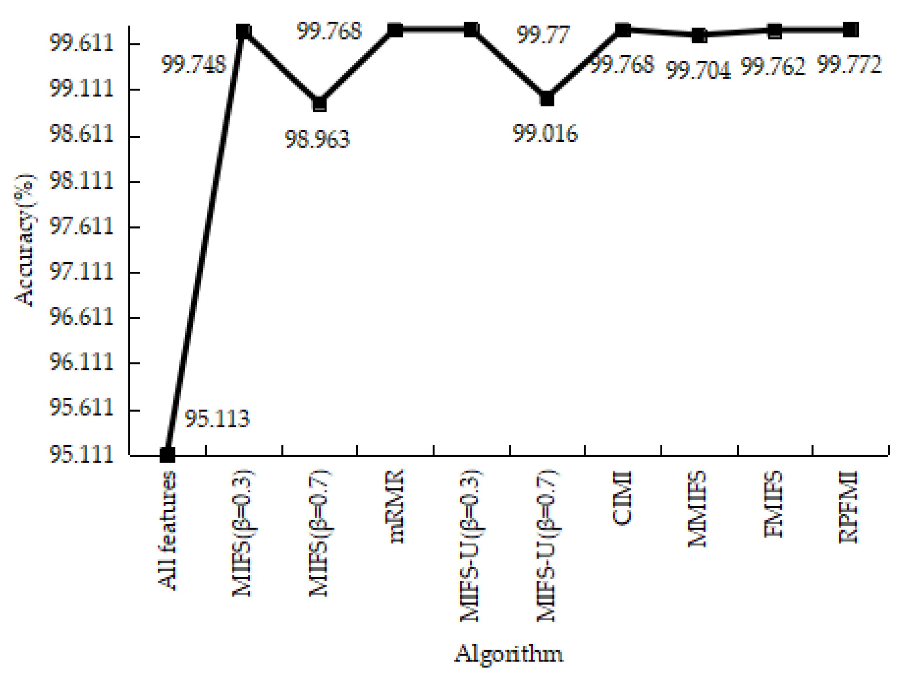
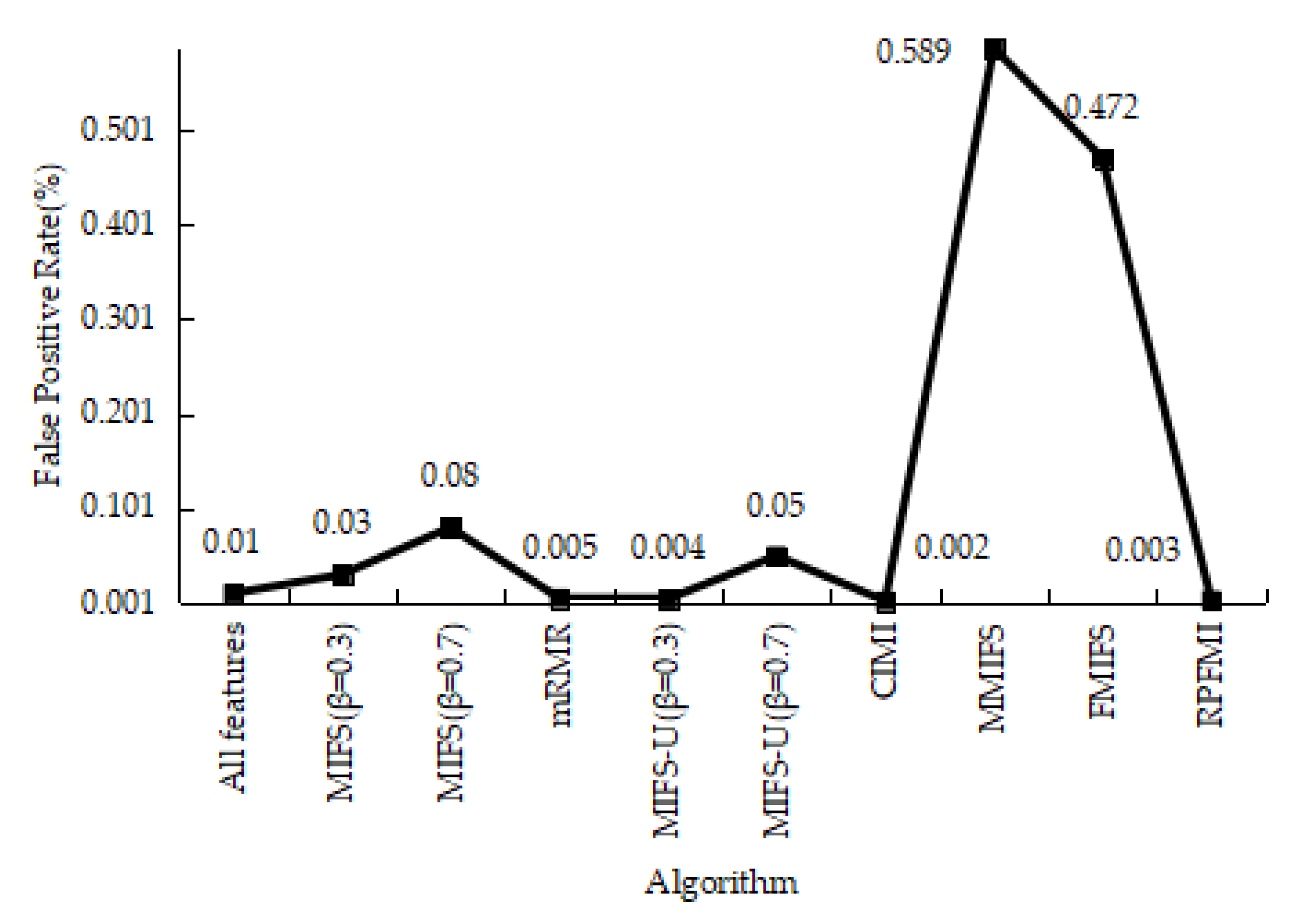
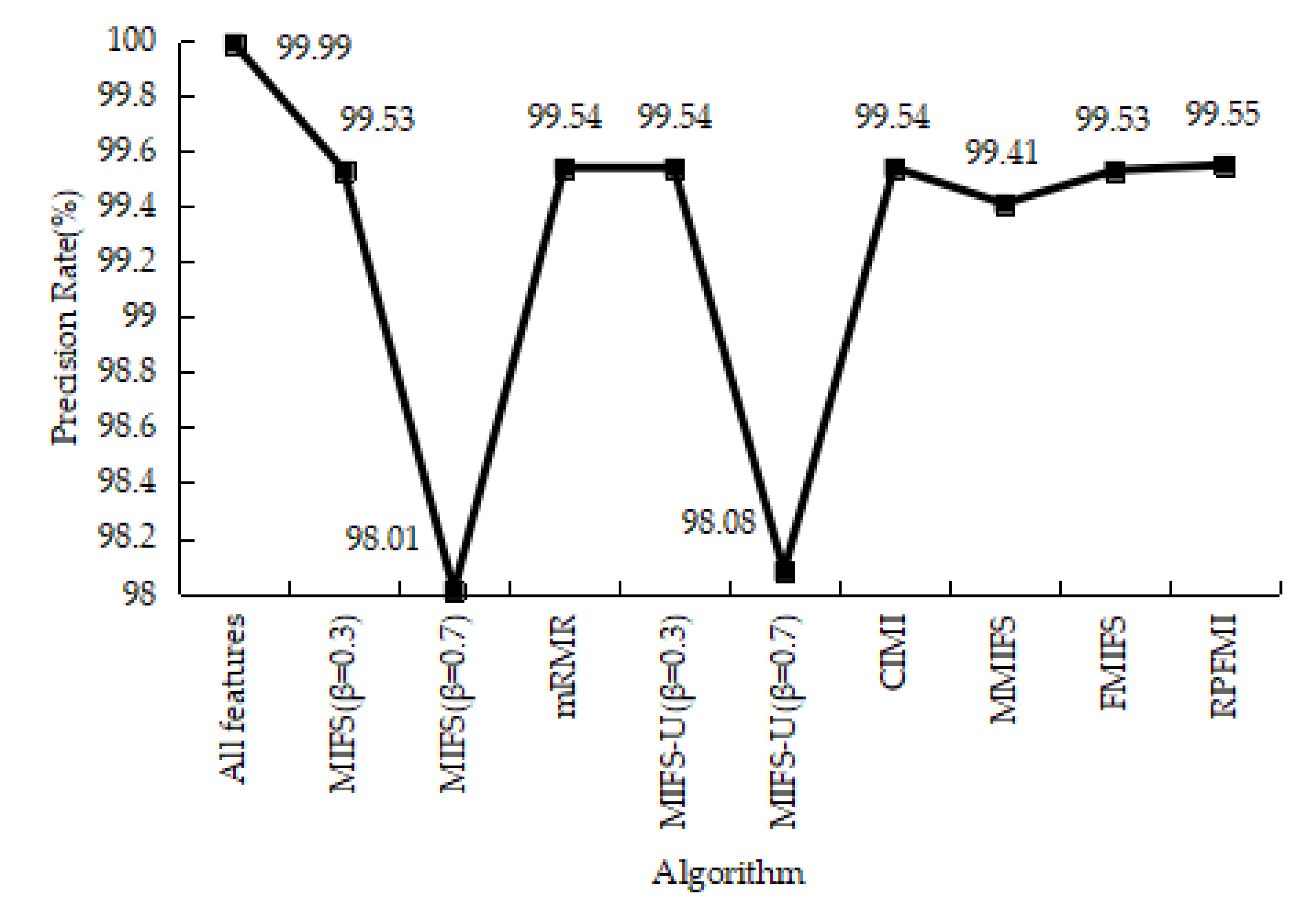
Table 6 shows the confusion matrices regarding the normal and DOS data in different models. It is obvious that the sum of the FP and FN in the RPFMI + SVM model is the smallest. Comparisons between different models in terms of the ACC, DR, FPR and PR are performed. Compared with the other feature selection algorithm, the highest ACC (i.e., 99.772%) can be obtained with the proposed algorithm (Figure 1). Figure 2 shows that RPFMI + SVM model has the same DR as other feature selection methods. The FPR of RPFMI + SVM is 0.003%, which is only larger than that of the CIMI model [22], as shown in Figure 3. Although the PR of the RPFMI model ranks second (Figure 4), it is higher than the other feature selection methods. Therefore, the RPFMI algorithm is advantageous over the other feature selection methods in improving both the ACC and PR and reducing the FPR.
4.3.2. User-to-Root Test Experiment
In this section, the detection performances of different models are shown for the U2R and normal samples in the test set. In the training phase, the numbers of normal samples and U2R samples are 1800 and 200, respectively, while in the testing phase, the numbers of normal samples and U2R samples are 1800 and 200, respectively.
In the U2R test data, due to the small amount of data, repeated sampling is used. The selected features with different feature selection methods are summarized in Table 7 and are used to detect U2R. It can be seen that the numbers of selected features with the MIFS (β = 0.3) [19], mRMR [20], MMIFS [32] and RPFMI algorithms are almost the same.
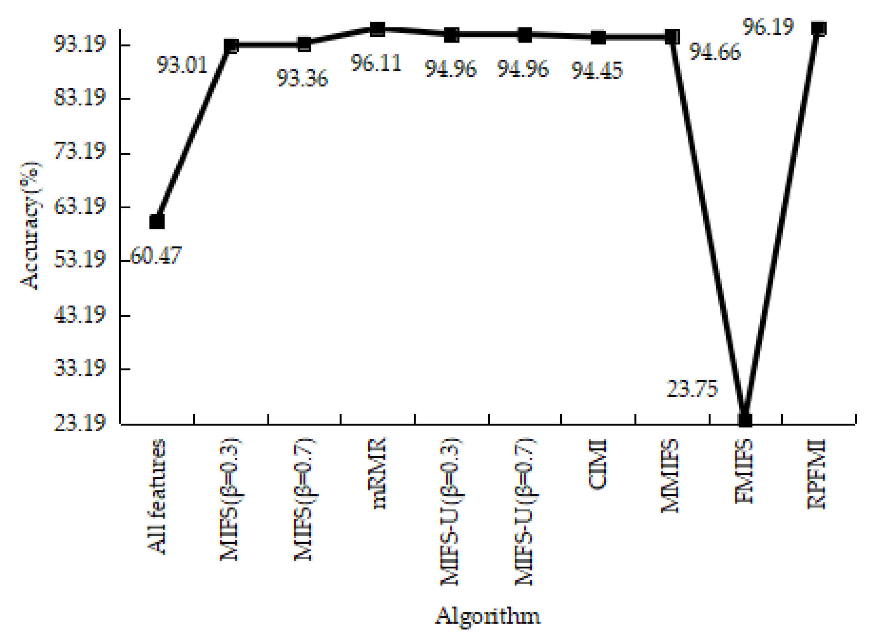
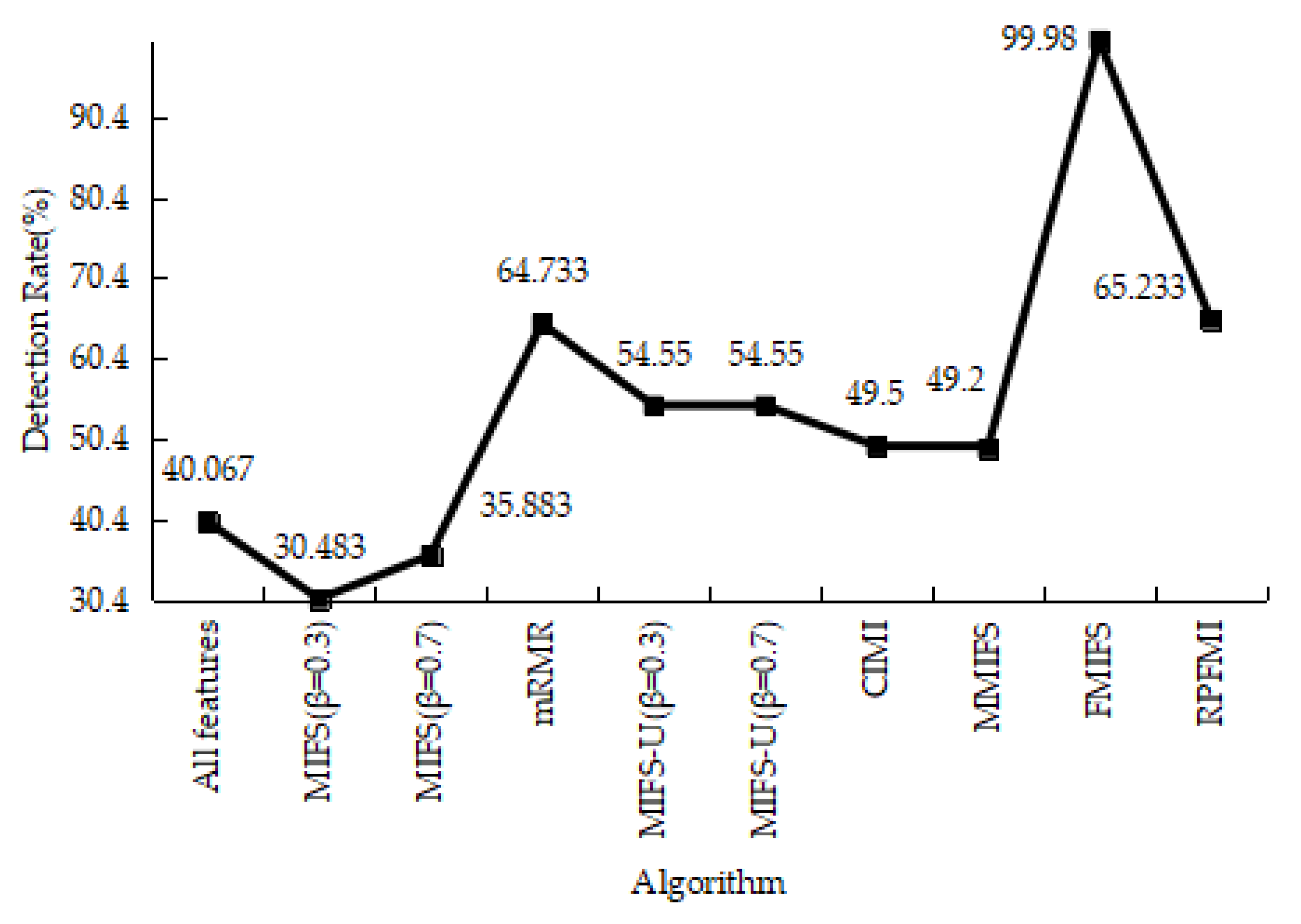
Table 8 shows the results of the confusion matrices for the normal and U2R data in different models. Among these 10 models, the RPFMI + SVM models has fourth largest TN and the second highest TP. The ACC, DR, FPR and PR with these models are illustrated. The highest ACC (i.e., 96.19%) is obtained with the RPFMI algorithm (Figure 5). Compared with the other models, the RPFMI model has the second highest DR (Figure 6) and the FPR of RPMI is only larger than those of the MIFS [19] and FMIFS [33] models (Figure 7). The RPRMI model ranks second in terms of the PR (Figure 8). Therefore, the proposed RPFMI algorithm demonstrates its ability to improve both the ACC and the PR.
4.3.3. Remote-to-Login Test Experiment
This section presents the detection performance of different models for the R2L and normal samples in the test set. In the training phase, the numbers of normal and R2L samples are 1800 and 200, respectively, while in the testing phase, the numbers of normal and R2L samples are 1800 and 200, respectively.
In Table 9, the selected features of the different feature selection methods, which are used to detect R2L, are summarized. It can be seen that the number of selected features with the RPFMI algorithm is smallest.
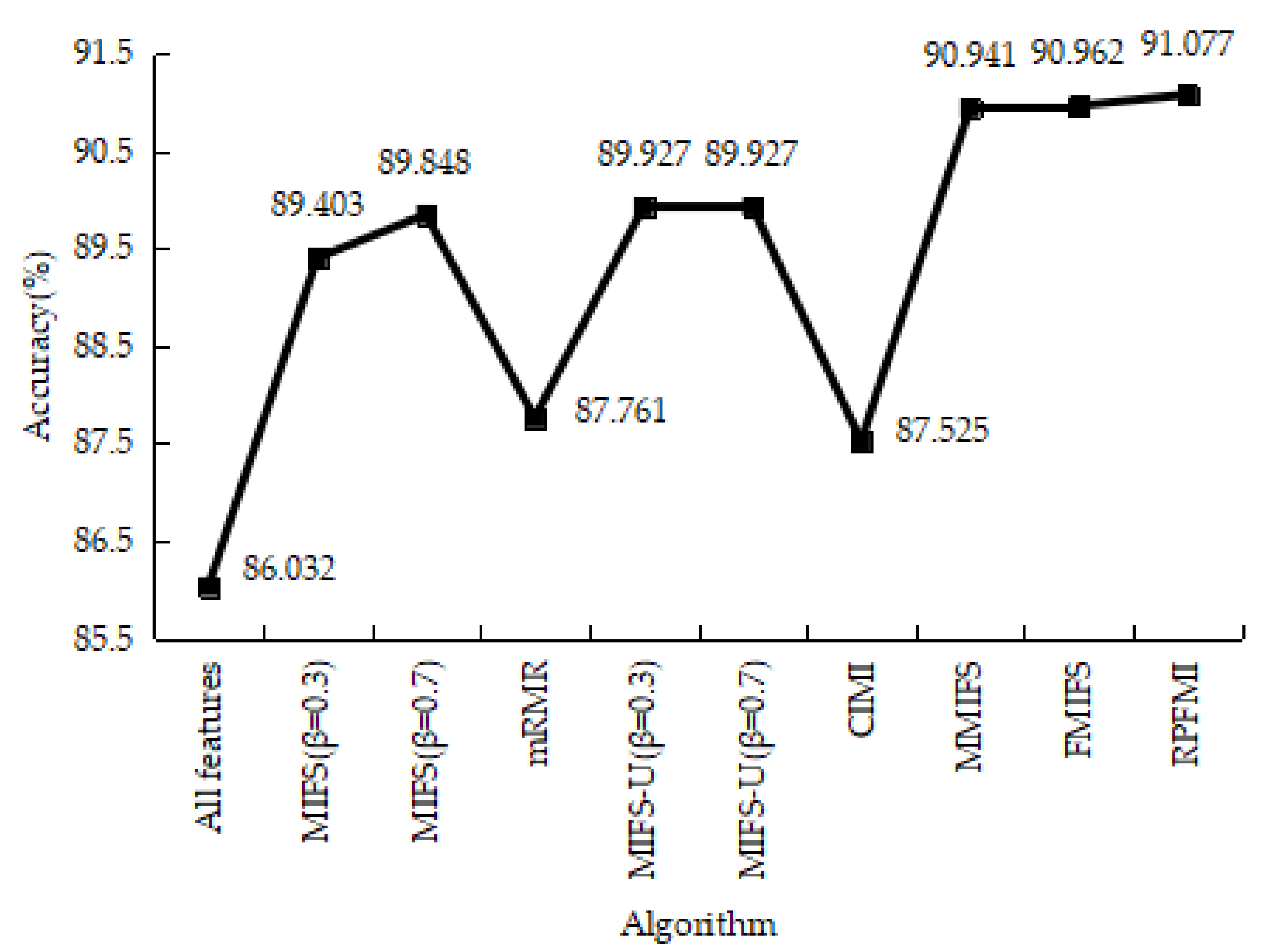
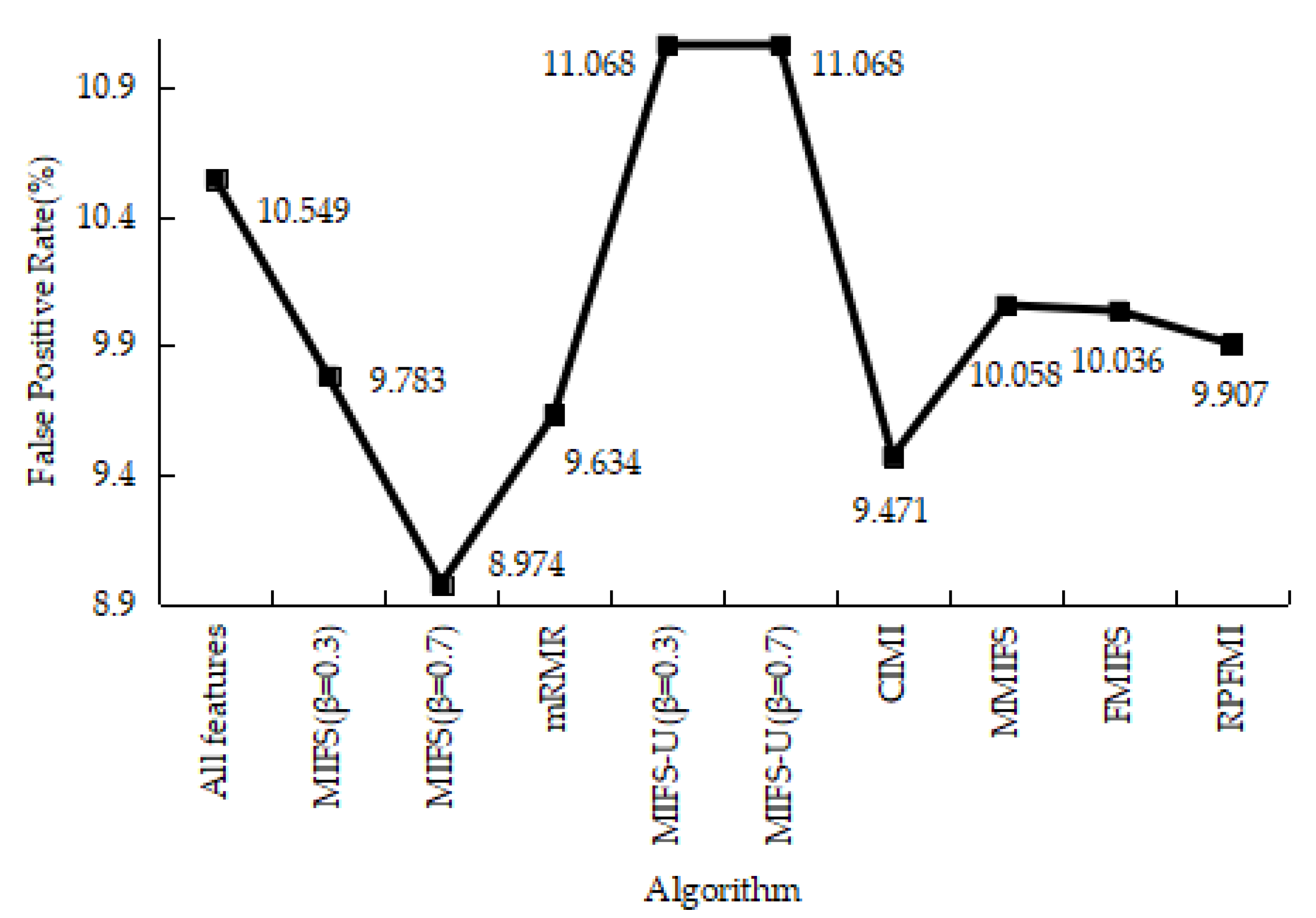
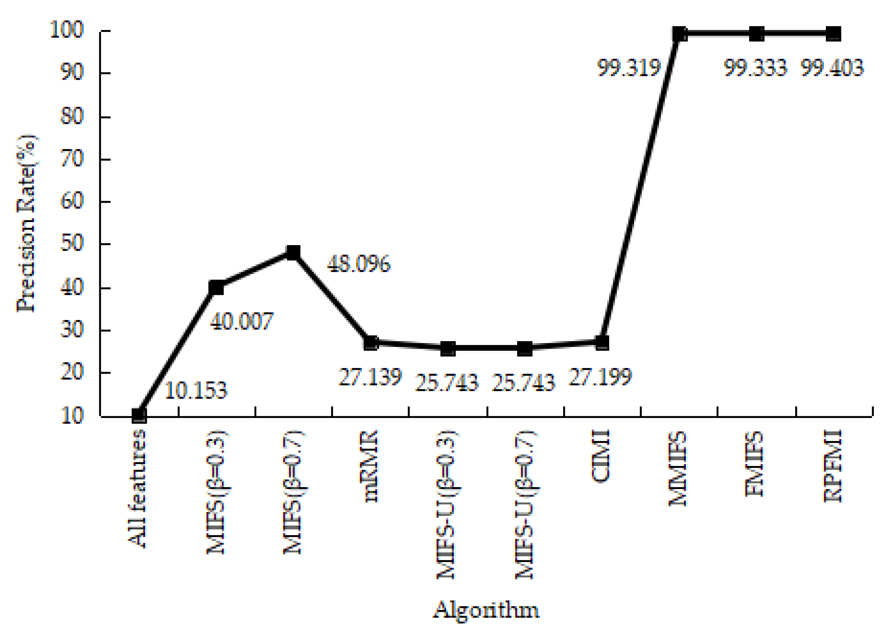
Table 10 shows the results of the confusion matrices for the normal and R2L data in different models. Among these methods, the RPFMI algorithm has the smallest FP and the largest TN. Comparisons between these methods regarding the ACC, DR, FPR and PR are carried out. The ACC of the RPFMI algorithm (i.e., 91.077%) is highest (Figure 9). Compared with other methods, the DR of the RPFMI algorithm ranks fourth in the DR (Figure 10), whereas its FPR is only larger than those of the MIFS [19], mRMR [20] and CIMI [22] algorithms (Figure 11). The largest PR obtained with the RPFMI algorithm (i.e., 99.403%) is also confirmed (Figure 12). In summary, the proposed RPFMI algorithm can improve the ACC and PR.
4.3.4. Kyoto 2006+ Test Experiment
This section presents the detection performances of different models for the attack and normal samples in the Kyoto 2006+ dataset of which the dataset in 2015 is used. In the training phase, the numbers of normal and attack samples are 10,000 and 10,000, respectively, while in the testing phase, the numbers of normal and attack samples are 2000 and 2000, respectively.
In Table 11, the selected features of the different feature selection methods, which are used to detect attacks, are summarized.
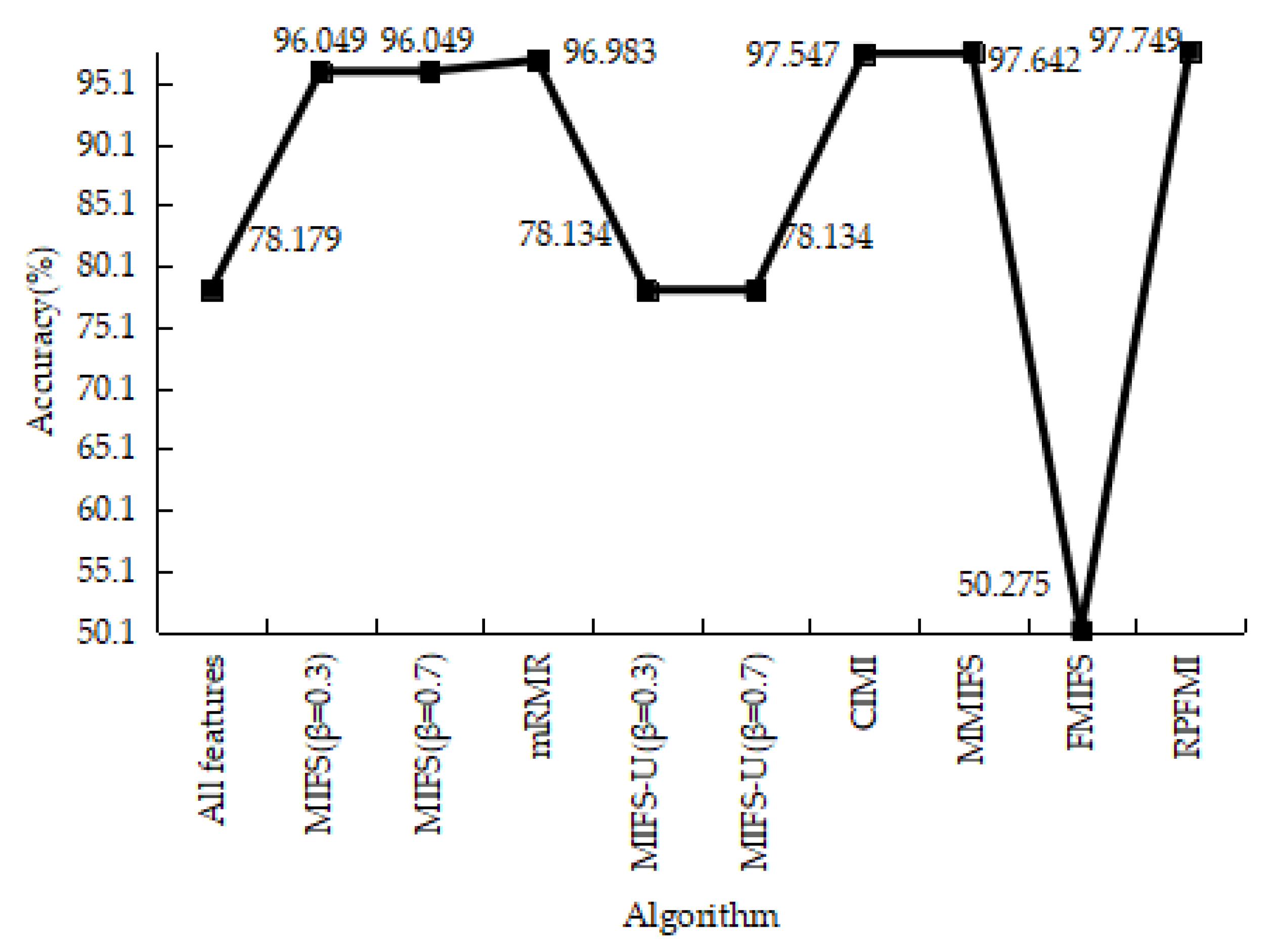
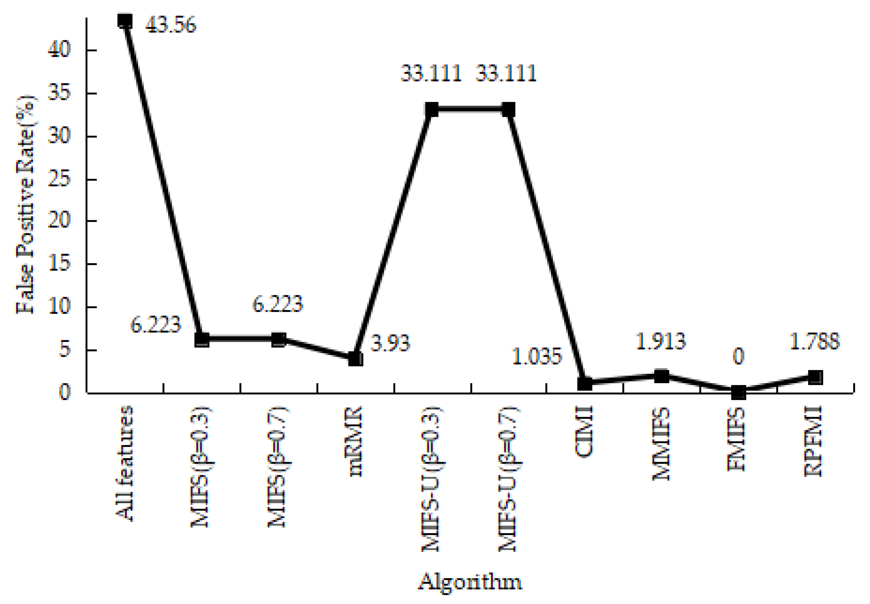
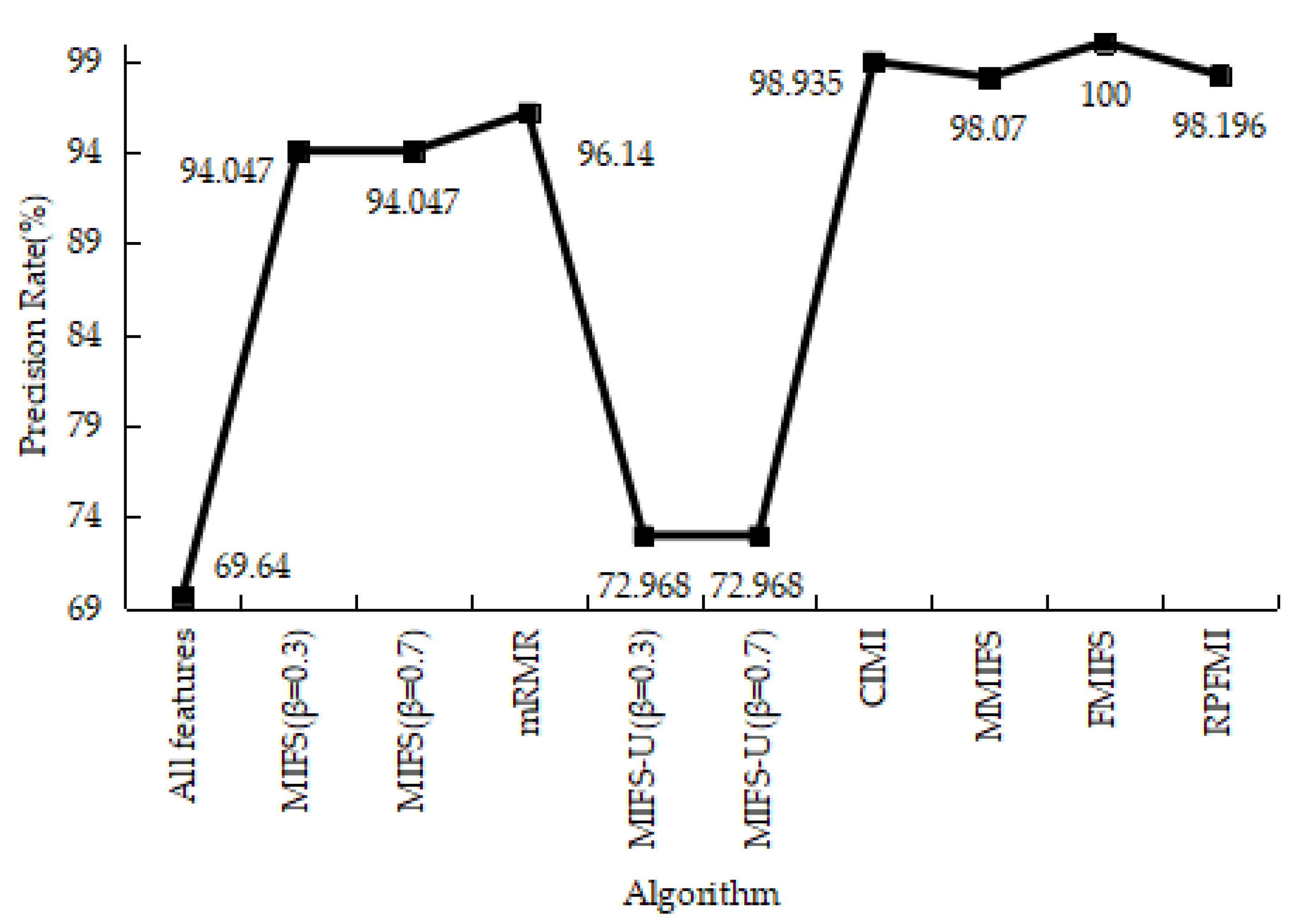
Table 12 shows the results of the confusion matrices with the normal and attack data in different models. It can be seen that the FP of the RPFMI + SVM model is only bigger than those of the CIMI [22] and FMIFS [33] models. The ACC, DR, FPR and PR of various models are presented. The ACC of the RPFMI algorithm (i.e., 97.749%) is highest (Figure 13). The DR of the RPFMI algorithm is higher than the MIFS-U [21], CIMI [22], MMIFS [32] and FMIFS [33] algorithms (Figure 14) and its FPR is only larger than the CIMI [22] and FMIFS [33] algorithms (Figure 15). In terms of the PR, the RPFMI algorithm ranks third among all the other methods (Figure 16). As a consequence, the ability of the proposed RPFMI algorithm to enhance the ACC and decrease the FPR has been verified.
4.3.5. Experiments Conclusion
There are DOS, U2R, R2L and Kyoto 2006+ test datasets in the experiments. These datasets are divided into 2 types. One type is large samples, such as DOS and Kyoto 2006+ datasets. The other type is small samples, such as U2R and R2L datasets. For large samples, the experiments show the proposed RPFMI algorithm can get best result in ACC using DOS and Kyoto 2006+ test datasets. For small samples, the experiments show the proposed RPFMI algorithm can get best result in ACC using U2R and R2L test datasets. Also, the experiments show it can get good result in PR on the premise of high ACC.
5. Conclusions and Future Work
In this paper, a new filter-based feature selection algorithm called the RPFMI algorithm, which is on a basis of MI, has been proposed. In this algorithm, three factors are considered: the redundancy between features, the impact between selected features and classes and the relationship between candidate features and classes. Through the proposed RPFMI algorithm, a good subset of features is selected to improve the accuracy of intrusion detection. Moreover the experiments show the proposed RPFMI algorithm can be well applied to large and small samples. For large samples, the proposed RPFMI algorithm can improve ACC. For small samples, the proposed RPFMI algorithm can improve ACC and get good result in PR on the premise of high ACC.
Author Contributions
F.Z. proposed the idea and conceptualization. F.Z. performed experiments, data analysis and scientific discussions and wrote the article. J.Z., X.N. and S.L. revised the clarity of the work as well as helping to write and organize the paper. Finally, Y.X. assisted in the proper preparations, English corrections and submission of the paper.
Funding
This research was supported in part by the National High Technology Research and Development Program of China (863 Program) under Grant 2015AA016005 and Grant 2015AA017201 and in part by the National Key Research and Development Program of China under Grant 2017YFB0802300.
Acknowledgements
The authors thank the reviewers for their valuable comments and suggestions, which improved the technical content and the presentation of the paper.
Conflicts of Interest
The authors declare no conflicts of interest.
References
- Singh, R.; Kumar, H.; Singla, R.K.; Ketti, R.R. Internet attacks and intrusion detection system: A review of the literature. Online Inf. Rev. 2017, 41, 171–184. [Google Scholar] [CrossRef]
- Xin, Y.; Kong, L.S.; Liu, Z.; Chen, Y.L.; Li, Y.; Zhu, H.; Gao, M.; Hou, H.; Wang, C. Machine Learning and Deep Learning Methods for Cybersecurity. IEEE Access 2018, 6, 35365–35381. [Google Scholar] [CrossRef]
- Wang, Z. Deep Learning-Based Intrusion Detection with Adversaries. IEEE Access 2018, 6, 38367–38384. [Google Scholar] [CrossRef]
- Karim, I.; Vien, Q.T.; Le, T.A.; Mapp, G. A comparative experimental design and performance analysis of Snort-based intrusion detection system in practical computer networks. MDPI Comput. 2017, 6, 6. [Google Scholar] [CrossRef]
- Inayat, Z.; Gani, A.; Anuar, N.B.; Khan, M.K.; Anwar, S. Intrusion response systems: Foundations, design, and challenges. J. Netw. Comput. Appl. 2016, 62, 53–74. [Google Scholar] [CrossRef]
- Chen, J.L.; Qi, Y.S. Intrusion Detection method Based on Deep Learning. J. Jiangsu Univ. Sci. Technol. 2017, 6, 18. [Google Scholar]
- Chung, I.F.; Chen, Y.C.; Pal, N. Feature selection with controlled redundancy in a fuzzy rule based framework. IEEE Trans. Fuzzy Syst. 2017, 26, 734–748. [Google Scholar] [CrossRef]
- Tao, P.Y.; Sun, Z.; Sun, Z.X. An Improved Intrusion Detection Algorithm Based on GA and SVM. IEEE Access 2018, 6, 13624–13631. [Google Scholar] [CrossRef]
- Zhang, T.; Ren, P.; Ge, Y.; Zheng, Y.; Tang, Y.Y.; Chen, C.P. Learning Proximity Relations for Feature Selection. IEEE Trans. Knowl. Data Eng. 2016, 28, 1231–1244. [Google Scholar] [CrossRef]
- Yan, B.H.; Han, G.D. Effective feature extraction via stacked sparse autoencoder to improve intrusion detection system. IEEE Access 2018, 6, 41238–41248. [Google Scholar] [CrossRef]
- Peng, H.C.; Long, F.H.; Ding, C. Feature selection for high-dimensional data: A fast correlation-based filter solution. In Proceedings of the 20th International Conference on Machine Learning, Washington, DC, USA, 21–24 August 2003. [Google Scholar]
- Mohamed, N.S.; Zainudin, S.; Othman, Z.A. Metaheuristic approach for an enhanced mRMR filter method for classification using drug response microarray data. Expert Syst. Appl. 2017, 90, 224–231. [Google Scholar] [CrossRef]
- Kohavi, R.; John, G. Wrappers for feature subset selection. Artif. Intell. 1997, 97, 273–324. [Google Scholar] [CrossRef]
- Hui, K.H.; Ooi, C.S.; Lim, M.H.; Leong, M.S.; Al-Obaidi, S.M. An improved wrapper-based feature selection method for machinery fault diagnosis. PLoS ONE 2017, 12, e0189143. [Google Scholar] [CrossRef] [PubMed]
- Dash, M.; Liu, H. Feature Selection for Classification. Intell. Data Anal. 1997, 1, 131–156. [Google Scholar] [CrossRef]
- Wang, L.M.; Shao, Y.M. Crack Fault Classification for Planetary Gearbox Based on Feature Selection Technique and K-means Clustering Method. Chin. J. Mech. Eng. 2018, 31, 4. [Google Scholar] [CrossRef] [Green Version]
- Viegas, E.K.; Santin, A.O.; Oliveira, L.S. Toward a reliable anomaly-based intrusion detection in real-world environments. Comput. Netw. 2017, 127, 200–216. [Google Scholar] [CrossRef]
- Jain, A.K.; Duin, R.P.W.; Mao, J.C. Statistical pattern recognition: A review. IEEE Trans. Pattern Anal. Mach. Intell. 2000, 22, 4–37. [Google Scholar] [CrossRef]
- Battiti, R. Using mutual information for selecting features in supervised neural net learning. IEEE Trans. Neural Netw. 1994, 5, 537–550. [Google Scholar] [CrossRef] [PubMed] [Green Version]
- Peng, H.; Long, F.; Ding, C. Feature selection based on mutual information: Criteria of max-dependency, max-relevance, and min-redundancy. IEEE Trans. Pattern Anal. Mach. Intell. 2005, 27, 1226–1238. [Google Scholar] [CrossRef] [PubMed]
- Kwak, N.; Choi, C.H. Input feature selection for classification problems. IEEE Tran. Neural Netw. 2002, 13, 143–159. [Google Scholar] [CrossRef] [PubMed]
- Novovičová, J.; Somol, P.; Haindl, M.; Pudil, P. Conditional Mutual Information Based Feature Selection for Classification Task; Springer: Berlin/Heidelberg, Germany, 2007. [Google Scholar]
- Guo, C.; Ping, Y.; Liu, N.; Luo, S.S. A two-level hybrid approach for intrusion detection. Neurocomputing 2016, 214, 391–400. [Google Scholar] [CrossRef]
- Jia, B.; Ma, Y.; Huang, X.H.; Lin, Z.; Sun, Y. A Novel Real-Time DDoS Attack Detection Mechanism Based on MDRA Algorithm in Big Data. Math. Probl. Eng. 2016, 2016, 1–10. [Google Scholar] [CrossRef]
- Kdd Cup 99 Intrusion Detection Dataset Task Description. University of California Department of Information and Computer Science, 1999. Available online: http://kdd.ics.uci.edu/databases/kddcup99/kddcup99.html (accessed on 20 December 2017).
- Wang, Y.W.; Feng, L.Z. Hybrid feature selection using component co-occurrence based feature relevance measurement. Expert Syst. Appl. 2018, 102, 83–99. [Google Scholar] [CrossRef]
- Boukhris, I.; Elouedi, Z.; Ajabi, M. Toward intrusion detection using belief decision trees for big data. Knowl. Inf. Syst. 2017, 53, 371–698. [Google Scholar] [CrossRef]
- Elshoush, H.T.; Osman, I.M. Alert correlation in collaborative intelligent intrusion detection systems-A survey. Appl. Soft Comput. 2011, 11, 4349–4365. [Google Scholar] [CrossRef]
- Tang, C.H.; Xiang, Y.; Wang, Y.; Qian, J.; Qiang, B. Detection and classification of anomaly intrusion using hierarchy clustering and SVM. Secur. Commun. Netw. 2016, 9, 3401–3411. [Google Scholar] [CrossRef]
- Chen, W.H.; Hsu, S.H.; Shen, H.P. Application of SVM and ANN for intrusion detection. Comput. Oper. Res. 2005, 32, 2617–2634. [Google Scholar] [CrossRef]
- Diosan, L.; Rogozan, A.; Pecuchet, J.P. Improving classification performance of support vector machine by genetically optimising kernel shape and hyper-parameters. Appl. Intell. 2012, 36, 280–294. [Google Scholar] [CrossRef]
- Amiri, F.; Yousefi, M.M.R.; Lucas, C.; Shakery, A.; Yazdani, N. Mutual information-based feature selection for intrusion detection systems. J. Netw. Comput. Appl. 2011, 34, 1184–1199. [Google Scholar] [CrossRef]
- Ambusaidi, M.A.; He, X.J.; Nanda, P.; Tan, Z. Building an intrusion detection system using a filter-based feature selection algorithm. IEEE Trans. Comput. 2016, 65, 2986–2998. [Google Scholar] [CrossRef]
- Brown, G.; Pocock, A.; Zhao, M.J.; Luján, M. Conditional Likelihood Maximisation: A Unifying Framework for Information Theoretic Feature Selection. J. Mach. Learn. Res. 2012, 13, 27–36. [Google Scholar]
- Brown, G. A New Perspective for Information Theoretic Feature Selection. In Proceedings of the International Conference on Artificial Intelligence & Statistics, Clearwater Beach, FL, USA, 16–18 April 2009; Volume 5. [Google Scholar]
- Kumar, S.; Sharma, A.; Tsunoda, T. An improved discriminative filter bank selection approach for motor imagery EEG signal classification using mutual information. In Proceedings of the 16th International Conference on Bioinformatics (InCoB)-Bioinformatics, Shenzhen, China, 20–22 September 2017. [Google Scholar]
- Bostani, H.; Sheikhan, M. Hybrid of binary gravitational search algorithm and mutual information for feature selection in intrusion detection systems. Soft Comput. 2017, 21, 2307–2324. [Google Scholar] [CrossRef]
- Aiello, M.; Mogelli, M.; Cambiaso, E.; Papaleo, G. Profiling DNS tunneling attacks with PCA and mutual information. Logic J. IGPL 2016, 24, 957–970. [Google Scholar] [CrossRef]
- Bhuyan, M.H.; Bhattacharyya, D.K.; Kalita, J.K. A multi-step outlier-based anomaly detection approach to network-wide traffic. Inf. Sci. 2016, 348, 243–271. [Google Scholar] [CrossRef]
- Song, J.; Takakura, H.; Okabe, Y.; Eto, M.; Inoue, D.; Nakao, K. Statistical analysis of honeypot data and building of Kyoto 2006+ dataset for NIDS evaluation. In Proceedings of the First Workshop on Building Analysis Datasets and Gathering Experience Returns for Security, Salzburg, Austria, 10 April 2011. [Google Scholar]
- Cheong, Y.G.; Park, K.; Kim, H.; Kim, J.; Hyun, S. Machine Learning Based Intrusion Detection Systems for Class Imbalanced Datasets. J. Korea Inst. Inf. Secur. Cryptol. 2017, 27, 1385–1395. [Google Scholar]
- Belhadj-Aissa, N.; Guerroumi, M. A New Classification Process for Network Anomaly Detection Based on Negative Selection Mechanism. In Proceedings of the 9th International Conference on Security, Privacy, and Anonymity in Computation, Communication and Storage (SpaCCS), Zhangjiajie, China, 16–18 November 2016. [Google Scholar]
- Kevric, J.; Jukic, S.; Subasi, A. An effective combining classifier approach using tree algorithms for network intrusion detection. Neural Comput. Appl. 2017, 28, 1051–1058. [Google Scholar] [CrossRef]
- Meena, G.; Choudhary, R.R. A review paper on IDS classification using KDD 99 and NSL KDD dataset in WEKA. In Proceedings of the International Conference on Computer, Communications and Electronics (Comptelix), Jaipur, India, 1–2 July 2017. [Google Scholar]
- Wan, M.; Shang, W.L.; Zeng, P. Double Behavior Characteristics for One-Class Classification Anomaly Detection in Networked Control Systems. IEEE Trans. Inf. Forensics Secur. 2017, 12, 3011–3023. [Google Scholar] [CrossRef] [Green Version]
- Kushwaha, P.; Buckchash, H.; Raman, B. Anomaly based intrusion detection using filter based feature selection on KDD-CUP 99. In Proceedings of the IEEE Region 10 Conference, Penang, Malaysia, 5–8 November 2017. [Google Scholar]
- Duan, S.; Levitt, K.; Meling, H.; Peisert, S.; Zhang, H. ByzID: Byzantine Fault Tolerance from Intrusion Detection. In Proceedings of the IEEE International Symposium on Reliable Distributed Systems, Nara, Japan, 6–9 October 2014. [Google Scholar]
- Rosas, F.; Chen, K.C. Social learning against data falsification in sensor networks. In Proceedings of the International Conference on Complex Networks and their Applications, Lyon, France, 29 November–1 December 2017. [Google Scholar]
Figure 1.
Accuracy on the DOS test data.

Figure 2.
Detection Rate on the DOS test data.
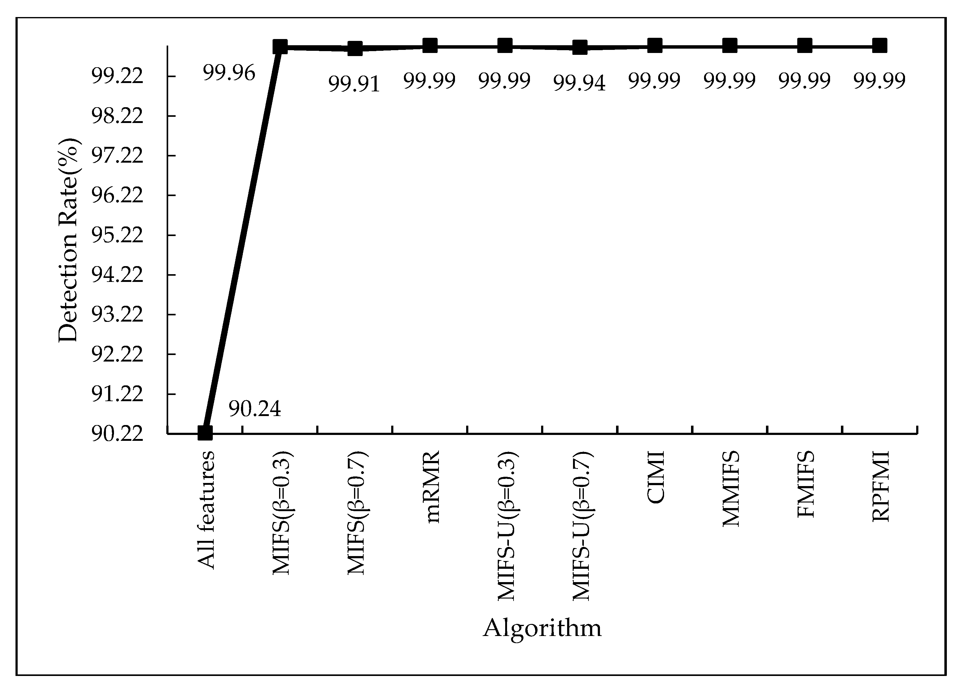
Figure 3.
False Positive Rate on the DOS test data.

Figure 4.
Precision Rate on the DOS test data.

Figure 5.
Accuracy on the U2R test data.

Figure 6.
Detection Rate on the U2R test data.

Figure 7.
False Positive Rate on the U2R test data.
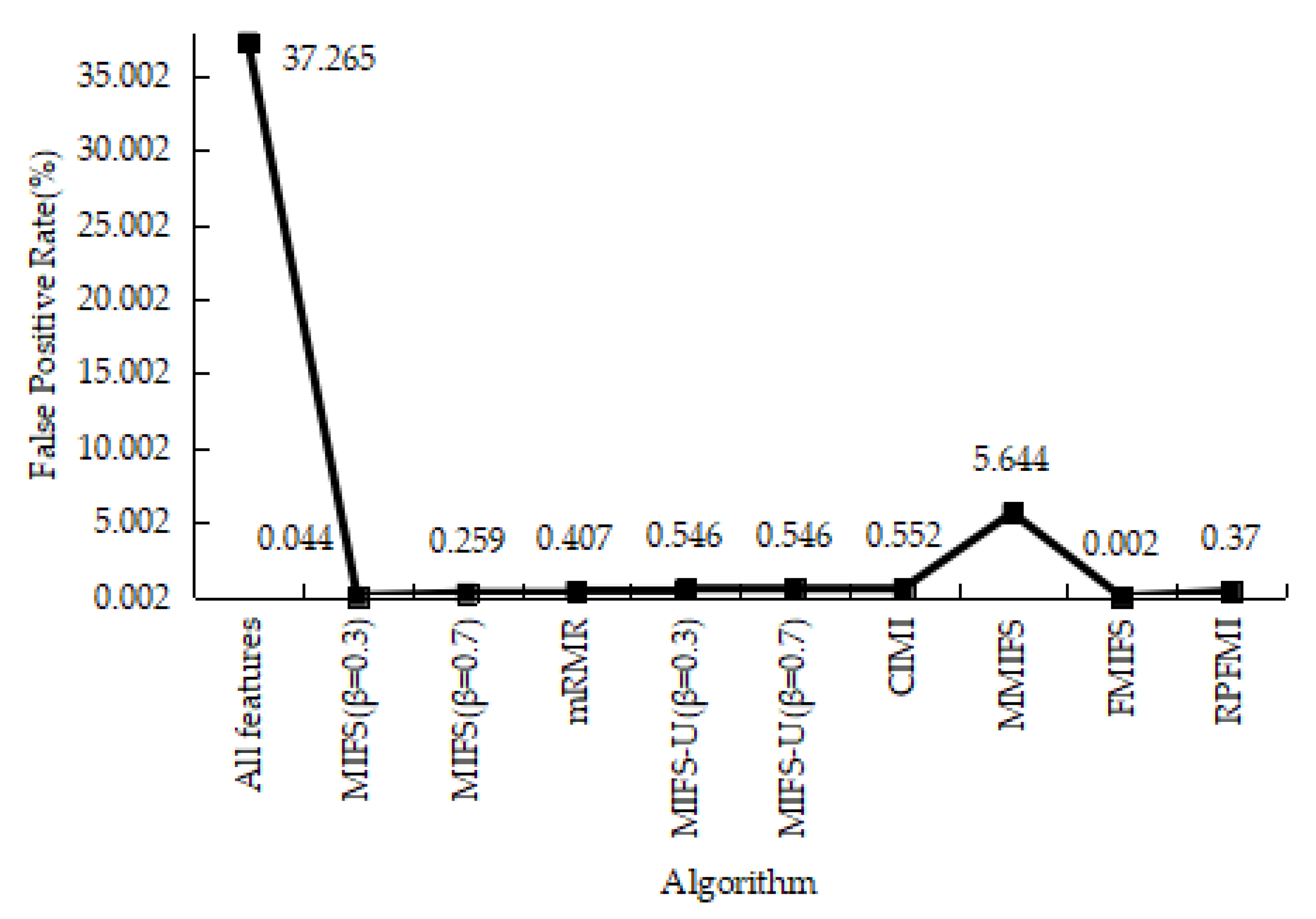
Figure 8.
Precision Rate on the U2R test data.
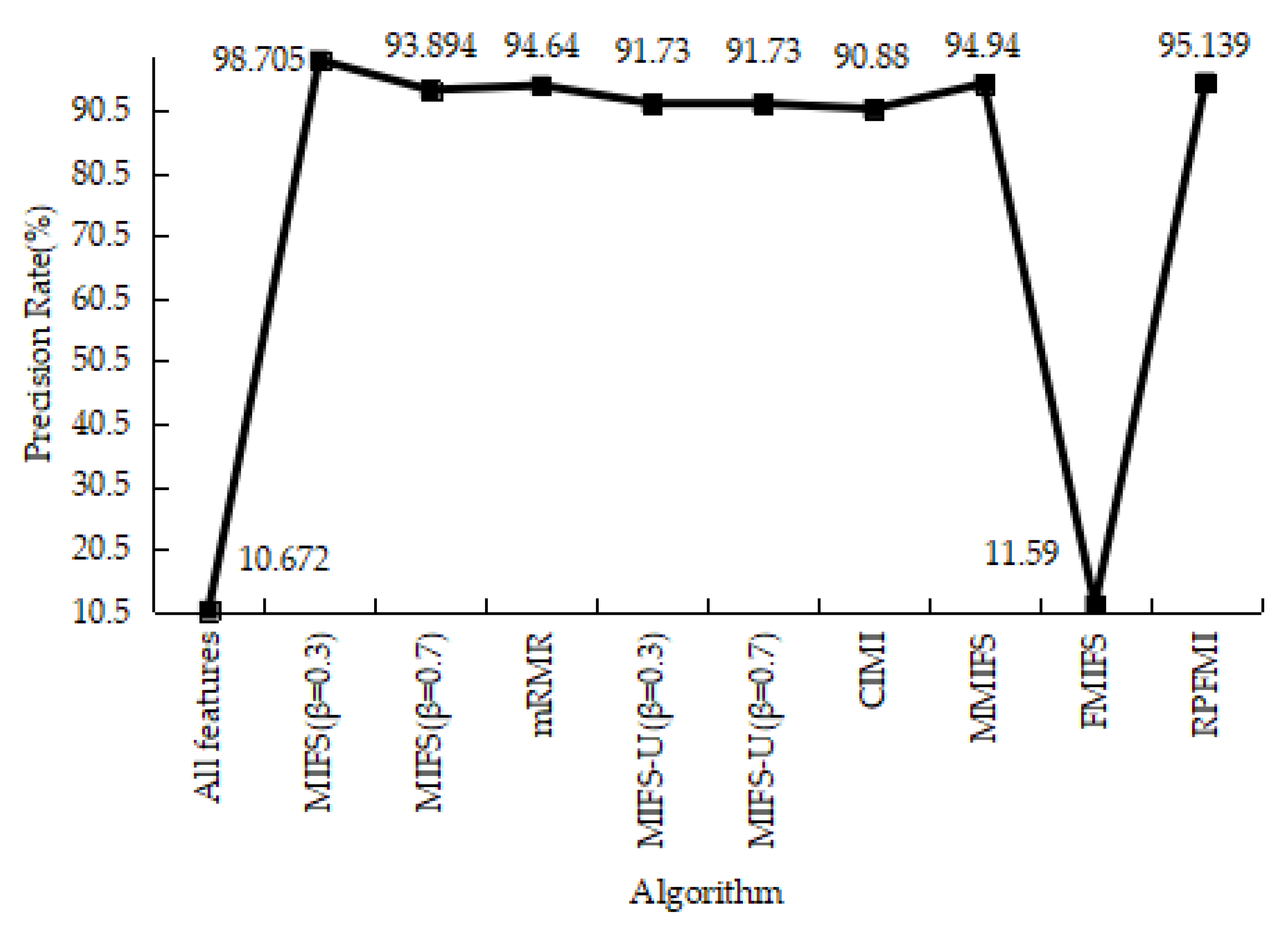
Figure 9.
Accuracy on the R2L test data.

Figure 10.
Detection Rate on the R2L test data.
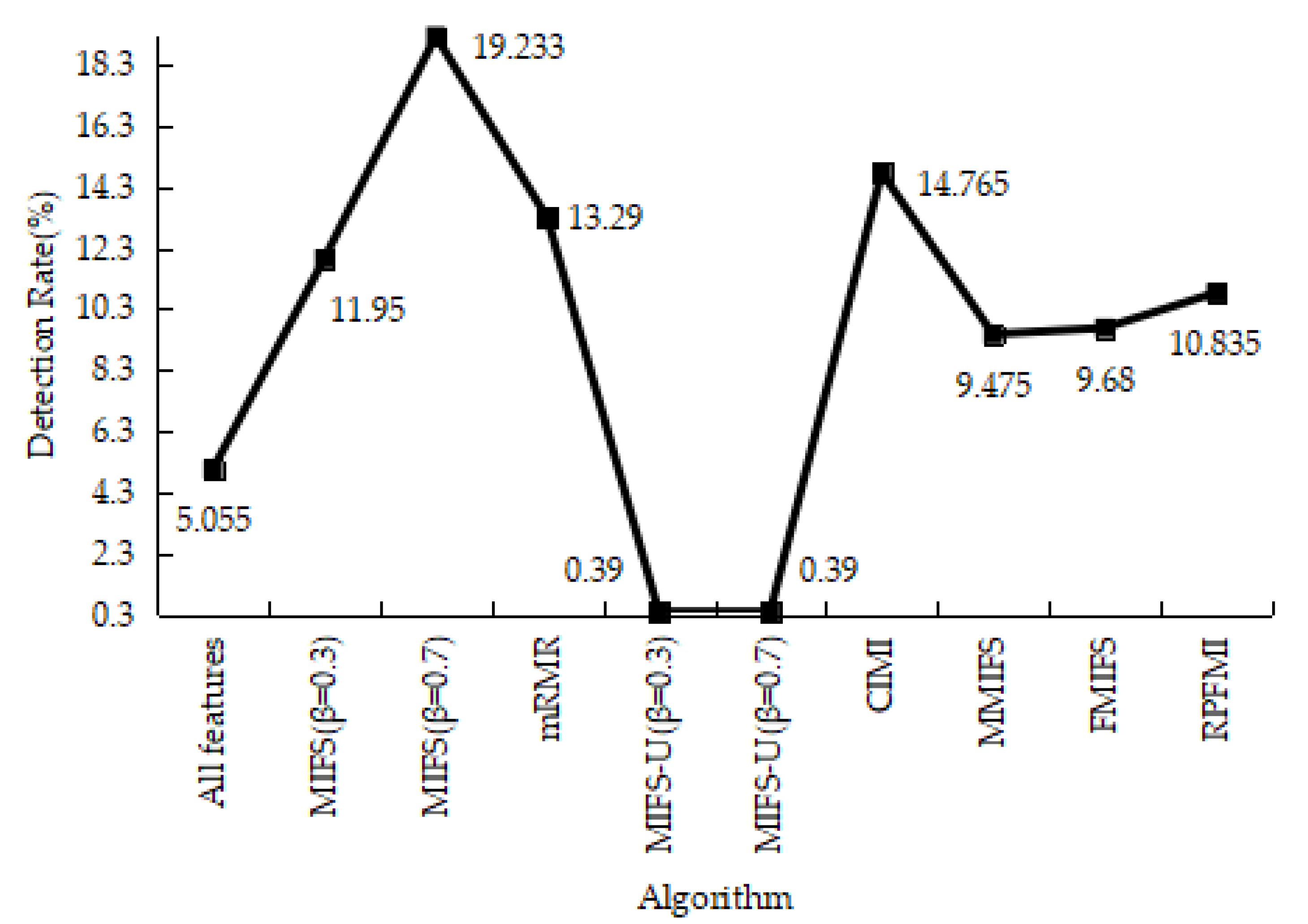
Figure 11.
False Positive Rate on the R2L test data.

Figure 12.
Precision Rate on the R2L test data.

Figure 13.
Accuracy on the Kyoto 2006+ test data.

Figure 14.
Detection Rate on the Kyoto 2006+ test data.
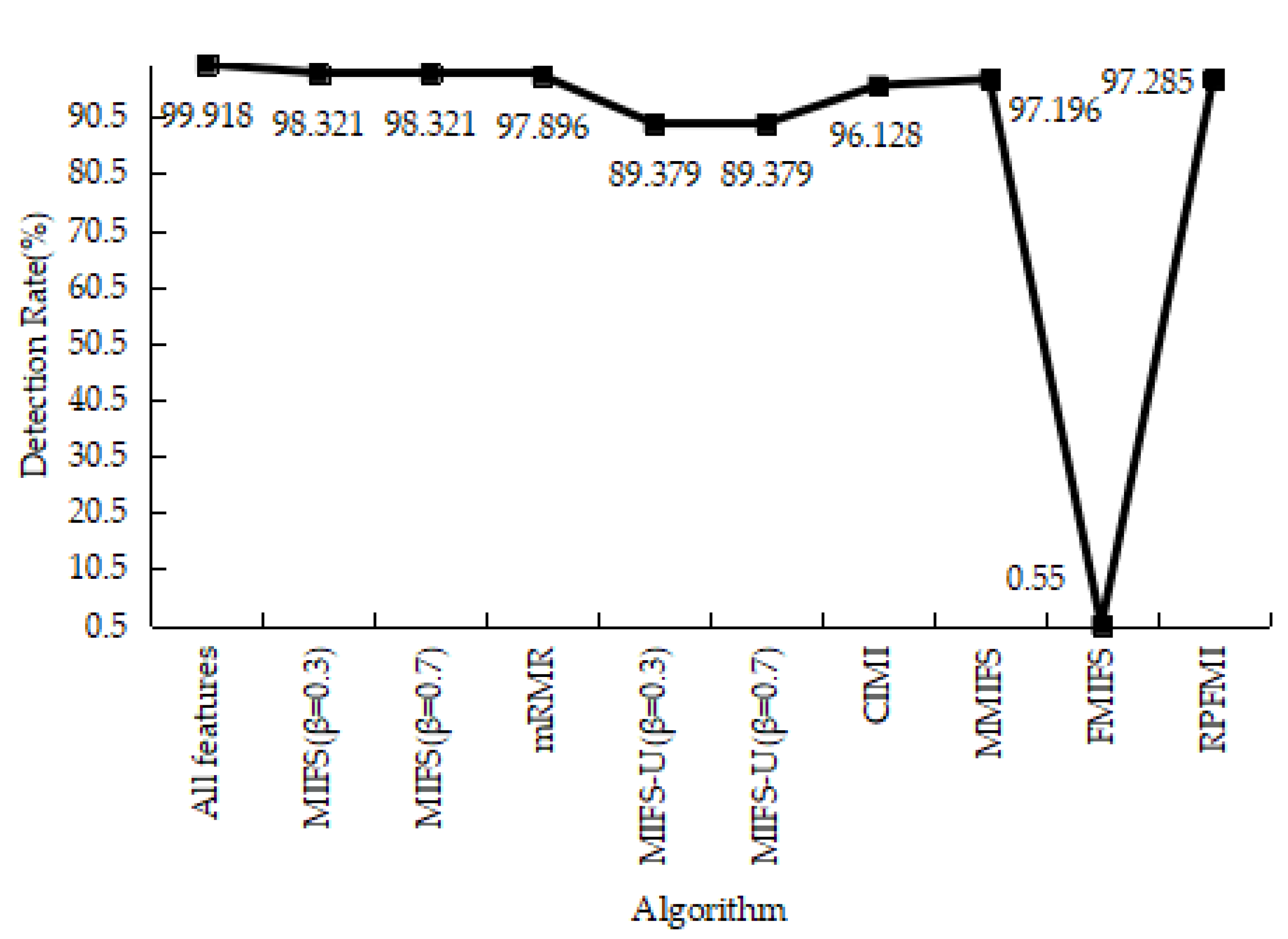
Figure 15.
False Positive Rate on the Kyoto 2006+ test data.

Figure 16.
Precision Rate on the Kyoto 2006+ test data.


Table 1.
The distribution of the 10% knowledge discovery and data mining (KDD) training data.
| Class | Number of Records | Percentage |
|---|---|---|
| Normal | 97,278 | 19.69 |
| DOS | 391,458 | 79.24 |
| U2R | 52 | 0.01 |
| Probe | 4107 | 0.83 |
| R2L | 1126 | 0.23 |
| Total | 494,021 | 100 |
Table 2.
The distribution of the KDD test data.
| Class | Number of Records | Number of Novel Attacks |
|---|---|---|
| Normal | 60,593 | — |
| DOS | 229,853 | 6555 |
| U2R | 228 | 189 |
| Probe | 4166 | 1789 |
| R2L | 16,189 | 10,196 |
| Total | 311,029 | 18,729 |
Table 3.
The nonnumeric feature conversion in the KDD Cup 99 data.
| Feature Name | Type Setting 1 | Type Setting 2 |
|---|---|---|
| protocol type = tcp | tcp = 1 | others = 0 |
| protocol type = udp | udp = 1 | others = 0 |
| protocol type = icmp | icmp = 1 | others = 0 |
| flag | SF = 1 | others = 0 |
Table 4.
Confusion matrix.
| Class | Predicted Negative Class | Predicted Positive Class |
|---|---|---|
| Actual negative class | True Negative (TN) | False Positive (FP) |
| Actual positive class | False Negative (FN) | True Positive (TP) |
Table 5.
Features selected by different feature selection algorithms using the denial of service (DOS) classifier.
Table 5.
Features selected by different feature selection algorithms using the denial of service (DOS) classifier.
| Model | Number of Features | Selected Features |
|---|---|---|
| ) [19] | 28 | 7, 2, 4, 19, 15, 16, 18, 17, 31, 14, 28, 23, 20, 26, 11, 27, 40, 3, 29, 1, 42, 13, 32, 38, 30, 39, 5, 41 |
| ) [19] | 31 | 7, 2, 19, 15, 16, 18, 17, 14, 23, 20, 31, 26, 28, 11, 27, 40, 29, 3, 1, 42, 39, 30, 4, 5, 32, 13, 41, 36, 38, 35, 34 |
| mRMR [20] | 11 | 7, 19, 2, 4, 28, 13, 3, 38, 31, 32, 40 |
| ) [21] | 23 | 7, 2, 13, 3, 32, 28, 19, 15, 18, 23, 31, 26, 16, 27, 20, 29, 14, 4, 11, 17, 40, 42, 38 |
| ) [21] | 31 | 7, 2, 31, 19, 15, 18, 23, 27, 28, 3, 16, 26, 20, 32, 14, 29, 11, 17, 40, 4, 30, 42, 39, 13, 5, 38, 41, 1, 36, 35, 37 |
| CIMI [22] | 17 | 7, 2, 13, 3, 32, 28, 19, 15, 18, 23, 31, 26, 16, 27, 20, 29, 14 |
| MMIFS [32] | 6 | 7, 2, 4, 13, 38, 3 |
| FMIFS [33] | 12 | 19, 15, 13, 31, 18, 20, 17, 38, 7, 4, 2, 16 |
| RPFMI | 23 | 7, 2, 13, 4, 19, 15, 16, 17, 18, 14, 28, 20, 23, 31, 29, 11, 26, 27, 40, 42, 3, 38, 1 |
Table 6.
Confusion matrices in different models using the DOS test data.
| Model | FP | FN | TN | TP |
|---|---|---|---|---|
| All features | 0.26 | 195.21 | 1999.74 | 1804.79 |
| MIFS ) [19] | 9.44 | 0.66 | 1990.56 | 1999.34 |
| MIFS ) [19] | 39.84 | 1.64 | 1960.16 | 1998.36 |
| mRMR [20] | 9.2 | 0.1 | 1990.8 | 1999.9 |
| MIFS-U ) [21] | 9.11 | 0.09 | 1990.89 | 1999.91 |
| MIFS-U ) [21] | 38.3667 | 0.9833 | 1961.633 | 1999.017 |
| CIMI [22] | 9.2667 | 0.0333 | 1990.733 | 1999.967 |
| MMIFS [32] | 11.78 | 0.07 | 1988.22 | 1999.93 |
| FMIFS [33] | 9.44 | 0.07 | 1990.56 | 1999.93 |
| RPFMI | 9.08 | 0.06 | 1990.92 | 1999.94 |
Table 7.
Features selected by different feature selection algorithms using the user to root (U2R) classifier.
Table 7.
Features selected by different feature selection algorithms using the user to root (U2R) classifier.
| Algorithm | Number of Features | Selected Features |
|---|---|---|
| ) [19] | 15 | 8, 9, 16, 21, 22, 23, 4, 27, 10, 12, 20, 19, 26, 39, 15 |
| ) [19] | 19 | 8, 9, 16, 21, 22, 23, 10, 4, 27, 12, 20, 19, 26, 17, 15, 5, 39, 14, 18 |
| mRMR [20] | 16 | 8, 9, 16, 21, 22, 23, 4, 27, 10, 39, 15, 12, 11, 18, 14, 19 |
| ) [21] | 3 | 8, 1, 2 |
| ) [21] | 3 | 8, 1, 2 |
| CIMI [22] | 2 | 8, 1 |
| MMIFS [32] | 14 | 8, 9, 16, 21, 22, 23, 4, 27, 39, 10, 15, 11, 18, 14 |
| FMIFS [33] | 9 | 8, 9, 16, 21, 22, 23, 27, 4, 10 |
| RPFMI | 16 | 8, 9, 16, 21, 22, 23, 10, 4, 27, 39, 15, 11, 14, 18, 12, 19 |
Table 8.
Confusion matrices in different models using the U2R test data.
| Model | FP | FN | TN | TP |
|---|---|---|---|---|
| All features | 670.7667 | 119.8667 | 1129.233 | 80.1333 |
| ) [19] | 0.8 | 139.0333 | 1799.2 | 60.9667 |
| ) [19] | 4.6667 | 128.2333 | 1795.333 | 71.7667 |
| mRMR [20] | 7.3333 | 70.5333 | 1792.667 | 129.4667 |
| ) [21] | 9.8333 | 90.9 | 1790.167 | 109.1 |
| ) [21] | 9.8333 | 90.9 | 1790.167 | 109.1 |
| CIMI [22] | 9.9333 | 101 | 1790.067 | 99 |
| MMIFS [32] | 5.2400 | 101.6 | 1794.76 | 98.4 |
| FMIFS [33] | 1525 | 0.0273 | 275 | 199.9727 |
| RPFMI | 6.6667 | 69.5333 | 1793.333 | 130.4667 |
Table 9.
Features selected by different feature selection algorithms using the R2L classifier.
| Algorithm | Number of Features | Selected Features |
|---|---|---|
| ) [19] | 14 | 8, 9, 10, 14, 15, 16, 19, 21, 22, 20, 4, 17, 12, 18 |
| ) [19] | 20 | 8, 9, 10, 14, 15, 16, 19, 21, 22, 20, 12, 18, 4, 17, 26, 27, 23, 31, 30, 11 |
| mRMR [20] | 12 | 8, 9, 10, 14, 15, 16, 19, 21, 22, 20, 4, 17 |
| ) [21] | 30 | 8, 1, 2, 3, 4, 5, 6, 7, 11, 12, 13, 17, 18, 20, 23, 24, 25, 26, 27, 28, 29, 30, 31, 32, 33, 34, 35, 36, 37, 38 |
| ) [21] | 30 | 8, 1, 2, 3, 4, 5, 6, 7, 11, 12, 13, 17, 18, 20, 23, 24, 25, 26, 27, 28, 29, 30, 31, 32, 33, 34, 35, 36, 37, 38 |
| CIMI [22] | 27 | 8, 1, 9, 10, 14, 15, 16, 19, 21, 22, 32, 3, 4, 17, 20, 12, 23, 6, 34, 38, 18, 26, 27, 11, 24, 37, 31 |
| MMIFS [32] | 10 | 8, 9, 10, 12, 15, 16, 21, 22, 14, 19 |
| FMIFS [33] | 8 | 8, 9, 10, 12, 15, 16, 21, 14 |
| RPFMI | 5 | 8, 9, 10, 12, 15 |
Table 10.
Confusion matrices in different models using the remote to login (R2L) test data.
| Model | FP | FN | TN | TP |
|---|---|---|---|---|
| All features | 89.47 | 189.89 | 1710.53 | 10.11 |
| MIFS () [19] | 35.84 | 176.1 | 1764.16 | 23.9 |
| MIFS () [19] | 41.51 | 161.535 | 1758.49 | 38.465 |
| mRMR [20] | 71.36 | 173.42 | 1728.64 | 26.58 |
| MIFS-U () [21] | 2.25 | 199.22 | 1797.75 | 0.78 |
| MIFS-U () [21] | 2.25 | 199.22 | 1797.75 | 0.78 |
| CIMI [22] | 79.04 | 170.47 | 1720.96 | 29.53 |
| MMIFS [32] | 0.13 | 181.05 | 1799.87 | 18.95 |
| FMIFS [33] | 0.13 | 180.64 | 1799.87 | 19.36 |
| RPFMI | 0.13 | 178.33 | 1799.87 | 21.67 |
Table 11.
Features selected by different feature selection algorithms.
| Algorithm | Number of Features | Selected Features |
|---|---|---|
| MIFS () [19] | 14 | 16, 4, 17, 14, 20, 15, 12, 7, 13, 8, 2, 11, 6, 19 |
| MIFS () [19] | 14 | 16, 4, 17, 14, 20, 15, 12, 7, 13, 8, 2, 11, 6, 19 |
| mRMR [20] | 7 | 16, 17, 4, 14, 20, 19, 2 |
| MIFS-U () [21] | 14 | 16, 1, 2, 3, 4, 5, 6, 7, 8, 9, 10, 11, 12, 13 |
| MIFS-U () [21] | 14 | 16, 1, 2, 3, 4, 5, 6, 7, 8, 9, 10, 11, 12, 13 |
| CIMI [22] | 4 | 16, 1, 19, 17 |
| MMIFS [32] | 7 | 16, 17, 4, 19, 14, 2, 3 |
| FMIFS [33] | 3 | 16, 17, 4 |
| RPFMI | 6 | 16, 17, 4, 14, 19, 2 |
Table 12.
Confusion matrices in different models using the Kyoto 2006+ test data.
| Model | FP | FN | TN | TP |
|---|---|---|---|---|
| All features | 871.2 | 1.64 | 1128.8 | 1998.36 |
| ) [19] | 124.46 | 33.58 | 1875.54 | 1966.42 |
| ) [19] | 124.46 | 33.58 | 1875.54 | 1966.42 |
| mRMR [20] | 78.6 | 42.09 | 1921.4 | 1957.91 |
| ) [21] | 662.22 | 212.42 | 1337.78 | 1758.58 |
| ) [21] | 662.22 | 212.42 | 1337.78 | 1758.58 |
| CIMI [22] | 20.69 | 77.45 | 1979.31 | 1922.55 |
| MMIFS [32] | 38.25 | 56.09 | 1961.75 | 1943.91 |
| FMIFS [33] | 0 | 1989 | 2000 | 11 |
| RPFMI | 35.75 | 54.31 | 1964.25 | 1945.69 |
© 2018 by the authors. Licensee MDPI, Basel, Switzerland. This article is an open access article distributed under the terms and conditions of the Creative Commons Attribution (CC BY) license (http://creativecommons.org/licenses/by/4.0/).
Share and Cite
MDPI and ACS Style
Zhao, F.; Zhao, J.; Niu, X.; Luo, S.; Xin, Y. A Filter Feature Selection Algorithm Based on Mutual Information for Intrusion Detection. Appl. Sci. 2018, 8, 1535. https://doi.org/10.3390/app8091535
AMA Style
Zhao F, Zhao J, Niu X, Luo S, Xin Y. A Filter Feature Selection Algorithm Based on Mutual Information for Intrusion Detection. Applied Sciences. 2018; 8(9):1535. https://doi.org/10.3390/app8091535
Chicago/Turabian StyleZhao, Fei, Jiyong Zhao, Xinxin Niu, Shoushan Luo, and Yang Xin. 2018. "A Filter Feature Selection Algorithm Based on Mutual Information for Intrusion Detection" Applied Sciences 8, no. 9: 1535. https://doi.org/10.3390/app8091535
Note that from the first issue of 2016, this journal uses article numbers instead of page numbers. See further details here.