Optimal Location of the Access Points for MIMO-UWB Systems


1
Department of School of Electric and Information Engineering, Qinzhou University, Qinzhou 535000, China
2
Department of Electrical Engineering, Tamkang University, Tamsui 25137, Taiwan
*
Author to whom correspondence should be addressed.
Appl. Sci. 2018, 8(9), 1509; https://doi.org/10.3390/app8091509
Submission received: 30 July 2018
/
Revised: 20 August 2018
/
Accepted: 26 August 2018
/
Published: 1 September 2018
(This article belongs to the Special Issue Selected Papers from IEEE ICICE 2018..)
Abstract
:Featured Application
Provide a secure, fast, and adaptable wireless transmission network for manufacturing systems.
Abstract
A multiple-input and multiple-output ultra-wideband (MIMO-UWB) system provides a higher data rate. However, the multipath effect of the intersymbol interference (ISI) increases the bit error rate (BER) and outage probability of the MIMO-UWB system. For this paper, the authors applied the real orthogonal design (ROD) to an MIMO-UWB system to improve the efficiency of that system. A ray-tracing technique and an inverse fast Fourier transform were used to get the impulse response of the indoor environment. In addition, a rake receiver was used to increase the strength of the received signal to minimize the multipath effect. For this paper, two cases of an indoor wireless MIMO-UWB system were studied: case (A) used different antenna arrays, whereas case (B) placed antenna arrays in different locations to find the best position of the transmitter. In case (A), three different shapes of antenna arrays, namely L-shape, circular-shape, and Y-shape, were used for the transmitter and receiver. The BER performance for these arrays in the UWB frequency of 3.1–10.6 GHz was examined. Numerical results showed that the outage probability of the circular array was better than that of the other two arrays. In case (B), the transmitter used was an array with two antenna elements. The optimal location for the transmitter was found by using both asynchronous particle swarm optimization (APSO) and self-adaptive dynamic differential evolution (SADDE). The numerical results indicated that the performance of APSO was better than that of SADDE.
1. Introduction
Ways and means to improve the quality of communication and to reduce its cost have become popular research topics in the field of wireless personal networks. It is expected that a combination of ultra-wideband (UWB) systems and multi-antenna systems will increase the transmission data rate. The UWB technology has the advantages of high-speed transmission, low-transmit power, low duty cycle, low-cost and simple transceiver structures, and less interference as compared to other applications. UWB is a valuable technology for future wireless applications such as indoor communication [1,2,3] and the intra-vehicular wireless sensor network (IVWSN) [4,5,6]. Indoor communication is limited to short distances and subjected to severe attenuation and multipath effect. In an IVWSN, the vehicle control systems and energy budgets of the sensor nodes in an in-car channel contain a large number of metal reflectors because of the short distance. Specifically, the distance between the transmitter and the receiver in an in-car channel is less than 10 m.
Smart antenna technology allows the device to collect more energy to improve the signal-to-noise ratio (SNR) at the receiver, while the multiple-input and multiple-output (MIMO) system has the advantage of high capacity gain [7,8,9,10,11]. MIMO systems are well-suited for working in diverse systems. In rich multipath channels, the probability of having more than one independent path increases. The properties of an MIMO channel, especially its capacity, are highly dependent on the spatial structure of the channel. Different diversity techniques have been applied to communication systems to improve their quality of communication [12,13,14,15].
UWB is mainly applied to indoor environments characterized by the multipath effect. The UWB technique has a plurality of diversity techniques and has almost exclusively been applied to MIMO to improve its quality of communication. The MIMO-UWB system has the potential for short-range, high-speed transmission requirements, and is especially suitable for complex indoor environments. It is a wireless solution that performs better in the current system design. MIMO-UWB has become a compelling candidate for extremely high data-rate communications [16,17,18,19].
This paper applies the real orthogonal design (ROD) [20,21], a diversity technique, in an MIMO-UWB system. Using an ROD to increase the transmit diversity scheme, the transmitter does not require any feedback from receivers. The computation complexity of the ROD is equal to maximal ratio receive combining.
Applying an ROD in an MIMO-UWB system addresses the market demands for quality and efficiency without requiring a significant redesign of existing UWB systems. The bit error rate (BER) performance is better when applying a high-order ROD. However, the intersymbol interference (ISI) effect is proportional to the size of the ROD. The multipath effect of the ISI, which increases the BER and outage probability, degrades the performance of an MIMO-UWB system. The rake receiver combines signals arriving on multiple propagation paths, and the tapped delay line (TDL) is used in this matched filter [22,23,24]. Therefore, a rake receiver is deployed to not only suppress the ISI multipath effect, but also utilize the energy present in multiple propagation paths.
Ray-tracing techniques are used to calculate the channel state information for different antenna radiation patterns [25]. The process can be carried out through simulation to overcome these drawbacks as long as the accuracy of the simulation tools can be proven. It conceptually assumes that a pincushion of rays is sent out from the transmitter, and is traced over the environments until either the ray has reached the receiver or the ray has lost enough power and its contribution to the received signal is negligible. The transmitting ray will be transmitted, reflected, or diffracted to the receiver. The receiver collects a narrowband signal around a given frequency range and converts it to the complex equivalent baseband signals.
For this paper, the authors used three different shapes of 8 × 8 antenna arrays (i.e., L-shape, circular-shape, and Y-shape arrays) for the transmitter and receiver. The BER performances for these arrays in MIMO-UWB communication systems are presented. To the best of the authors’ knowledge, there is still no published work using asynchronous particle swarm optimization (APSO) and self-adaptive dynamic differential evolution (SADDE) to search for transmission locations to minimize the outage probability of indoor wireless communication channels. In this paper, two different optimization algorithms are proposed and compared to find the optimal transmitter location for the MIMO-UWB communication system [26,27,28]. The outage probability of the MIMO-UWB systems is investigated. The MIMO-UWB system and its bit error rate calculation formula are described in Section 2.1. APSO and the SADDE evolution algorithms are described in Section 2.2. The results of applying different shape of antenna arrays and finding an optimal transmitter location by applying APSO and SADDE are shown and discussed in Section 3.
2. Method
2.1. System Description
UWB combined with MIMO is a viable way to achieve high data rates in wireless communication. The authors focused on the application of RODs, because they are key to achieving low BER and cost reduction in MIMO-UWB systems. A plurality of complex orthogonal designs for narrowband is available in the literature [20,24].
Figure 1 shows the basic idea of a binary pulse amplitude modulation (BPAM) for a UWB system consisting of NT transmitting and NR receiving antennas with NF rake fingers. Each information symbol is being conveyed through monocycle pulses with a period of Td and with different polarities. A frame is associated with a set of slots. Multi-antenna systems provide a diversity order without any feedback signal from the receiver to the transmitter. Diversity techniques are used to mitigate degradation in the error performance of the radio channel without using additional radiated power or spectral bandwidth [29]. The transmit symbols are applied to the ROD [20,21], where each symbol with a slot time Ts seconds is pulse-shaped by the second order of Gaussian waveform in the transmitters.
The received signal Y(t) passes through a matching filter whose impulse response is hij(t) and the sampled signal in the first frame is divided into two branches. These signals are fed to the rake receiver and combined with the MRC algorithm, producing signals r1(t) and r2(t) respectively. Finally, the transmitted symbols S1(t) and S2(t) can be independently decoded from the output r(t). The same procedure is repeated for the next frame. The signals Ŝ(t) are summed up to collect all the diversities provided by multiple receive antennas, multi-time slot, and multipath. The figure shows that the inherent diversity of UWB signals in the temporal domain is collected by the rake receiver, while the diversity in the spatial domain is harvested by the use of the space–time code (STC). It is beneficial to employ an ROD code for collecting more diversities.
An ROD of size n is an n by n orthogonal square matrix with entries in the indeterminate ±S; the rows of the matrix represent antennas, whereas its columns represent transmission time slots [24,30]. The ROD of size 2 is as shown below:
S1 and S2 are two information symbols transmitted simultaneously from two transmitted antennas (NT = 2). Then, the authors attempted to detect the information symbols S1 and S2 based on the consecutive time slot 1 and time slot 2 (Nslot = 2). Finally, they combined all the spatial diversities provided by the receiving antennas (NR = 2) and the signal components that propagated through the channel by different paths.
The ROD codes were developed, and the decoding algorithm was given. Based on the Hurwitz-Radon theorem, the full rate can be achieved by using RODs of size 8, that is, with eight transmitted antennas [20,24]. The ROD of size 8 is as shown below:
For this paper, an impulse radio with a BPAM was applied. Time-modulated UWB communication is based on the discontinuous emission of a very short waveform as a train of pulses. Each pulse has ultra-wide spectral requirements in the frequency domain. Because the pulse propagates well in the radio channel, it does not require additional carrier modulation. This radio concept is referred to as impulse radio.
The transmitted PAM signals are as follows:
where Sj is the transmitted signal of transmitter j, Td is the transmitting signal duration, and the value of Td is usually much larger than the pulse duration. Es is the average transmitted energy per symbol. In a BPAM, each symbol takes only two values S = {+1,−1} and is assumed to be independent and identically distributed (i.i.d.). The second derivative of the Gaussian waveform is used here as the transmit waveform p(t) at the nanosecond scale. The second derivative of Gaussian waveform p(t) can be described by the following expression:
where σ is the standard deviation of the Gaussian wave
The channel state information (CSI) is available at the receiver, which is the channel impulse response between a receiving antenna and a transmitting antenna. A ray-tracing channel model was developed to calculate the channel state information for the UWB-MIMO system.
The ray-tracing technique can deal with radio wave propagation in any environment. A ray-tracing approach based on frequency domain was applied to the deterministic simulation for the indoor channel. A pincushion of rays was sent out from the transmitter and traced over a given environment until either it had reached the receiver or it had lost enough power, and its contribution to the received signal was negligible. During transmission, the ray was transmitted, reflected, or diffracted before reaching the receiver. The receiver collected a narrowband signal around the given frequency range and converted the signal to a complex equivalent baseband signal. The goal of channel modeling was to determine the impulse response for any given transmitter-receiver location in the system.
where hij is the channel impulse response between a receiving antenna i and a transmitting antenna j, L is the path index, βij,L and τij,L are the amplitude and the time delay of L-th path between receiving antenna i and transmitting antenna j. NL is the number of paths.
The impulse response with input transmitted signal S(t) and received signal Y(t) is described by convolution. The corresponding received signals are as follows:
where * denotes the convolution operator.
After receiving the signals through the channel, they are processed with a correlator in receivers with rake finger NF. With rake receivers, the ability to improve the received signal can be increased in multi-path fading channels. The different signal paths propagated by different paths are combined by rake receivers [31,32,33]. These programs produce time diversity. Combining different signal components increases the signal-to-noise ratio (SNR) and also improves the link performance. The rake receiver is designed to compensate the UWB channel’s multipath. It is assumed that the receiver noise n(t) at the corresponding time instant, including the effect of correlation, is Gaussian white noise with zero mean and variance N0/2. The probability of BER can be represented as [24]:
where αij,f is the corresponding receiving amplitude for Sj at receiver antenna i with rake finger f, and erfc is the complementary error function.
Making the generalization for the case with the ROD of size 8 and rake receiver, the BER formula is as follows:
Alternatively, the outage probability can also be used for evaluating the system. The bit error rate (BER) is an essential factor when calculating the outage probability in an MIMO-UWB system. The receiver is defined as the “outage point” as its BER > 10−6. The definition of the outage probability is as follows [25,34]:
2.2. Evolution Algorithms
The following two algorithms were used to minimize the value of the objective function (OF), which is defined in Equation (7).
2.2.1. Self-Adaptive Dynamic Differential Evolution
The SADDE is based on the DDE scheme with the ability to automatically adjusting scaling factors without increasing the time complexity [28,35]. The SADDE algorithm starting from the initial population consists of a randomly generated set of individual coordinates that represent each location of the transmitter antenna. The SADDE algorithm contains the following steps:
Step 1: According to the problem, initialize the population of a set of D-dimensional vectors in the starting population, parameter space is , where D is the number of parameters to be optimized, and Mp is the population size.
Step 2: Evaluate the objective function (7) for each individual in the population.
Step 3: The mutation operation is performed by an arithmetic combination of individuals. Each trial vector is generated from the parent’s generation parameter vector according to the following equation:
where and are the scaling factors associated with the vector differences and , respectively. The disturbance vector V of the mutation mechanism consists of the parameter vector , the best particle , and two randomly selected vectors, and , which are adjusted automatically.
Control parameters in SADDE continue to evolve from generation to generation. The new vector is generated by using the evolution values of the control parameters. During the selection process, these new carriers have a better chance of surviving and passing improved control parameters to the next generation. Each generation’s control parameters for each individual here are self-adjusting according to the following scheme:
where and are the lower limits of and , their values being set at 0.1. and are the upper limits of and , and their values are set at 0.9 [28,36]; rand1, rand2, rand3, and rand4 are random numbers with values uniformly distributed between 0 and 1.
Step 4: Perform crossover operations to increase the diversity of parameter vectors. The cross vector is replaced by the current vector or trial vector based on the probability of crossover . It can be expressed as follows:
where is the random number generated uniformly between 0 and 1. is the crossover probability, . Rand5 and rand6 are random numbers with the values uniformly distributed between 0 and 1. is the crossover probability, . The bigger the value of , the more rapidly the termination criteria can be reached. However, a smaller value of increases the diversity of the parameter vectors.
Step 5: The selection operation is used to generate offspring. Compare the parent vector with the cross vector and select the vector with the smaller objective function value as the next generation member. The selection operation is shown below:
SADDE is a self-adaptive evolutionary algorithm. Specifically, if the offspring has a better objective function value than its parent, then this offspring individual can be used to replace each parent. If there are individuals in the offspring that meet the termination criteria, stop this process and get the best individual; otherwise, return to step 2 to continue the entire cycle.
2.2.2. Asynchronous Particle Swarm Optimization
Asynchronous particle swarm optimization (APSO), proposed by Clerc, is an alternative to the particle swarm optimization (PSO) algorithm [36]. APSO uses a different velocity update equation, which utilizes a parameter called constriction factor. The purpose of the constriction factor is to improve the convergence. As APSO updates the global best particle position as soon as one is found that is less than the value of the objective function. APSO will converge more quickly than PSO. For this paper, APSO contains six steps in minimizing the value of the objective function, as shown below.
The number of particles Xi (i = 1, 2, …, Np) with D dimensional vectors is chosen, where D is the number of parameters to be optimized, and Np is the population size:
Step 1: Randomly set the initial particle position based on the search range.
Step 2: Evaluate the value of the objective function for each particle and record the particle information, that is, the particle position which has a value less than the current value of the objective function, and the new and smaller value of the objective function.
Step 3: Update the global best particle position xgb and best particle position xpb for the gth generation based on the data recorded in Step 2.
Step 4: Ten percent of xgb will be mutated by the following equation:
where c1 and c2 are the scaling parameters. Both φ1 and φ2 are random real numbers from zero to one. g (g = 1, 2, 3, ..., gmax) is the current iteration number. The space limit of the environment is between xmax and xmin. If the objective function of the mutation particle is the best, update the xgb with xmu.
Step 5: Calculate the particle velocity using the following equation:
where ij is the ith particle and jth dimension, is the constriction factor, , c3 is set as 2.8 and c4 is set as 2.8, c3 and c4 are both positive constants, and 1.3 to control the impact of the local and global component in velocity;
Step 6: Stop the algorithm and output the final data when the termination criteria have been reached.
3. Numerical Results
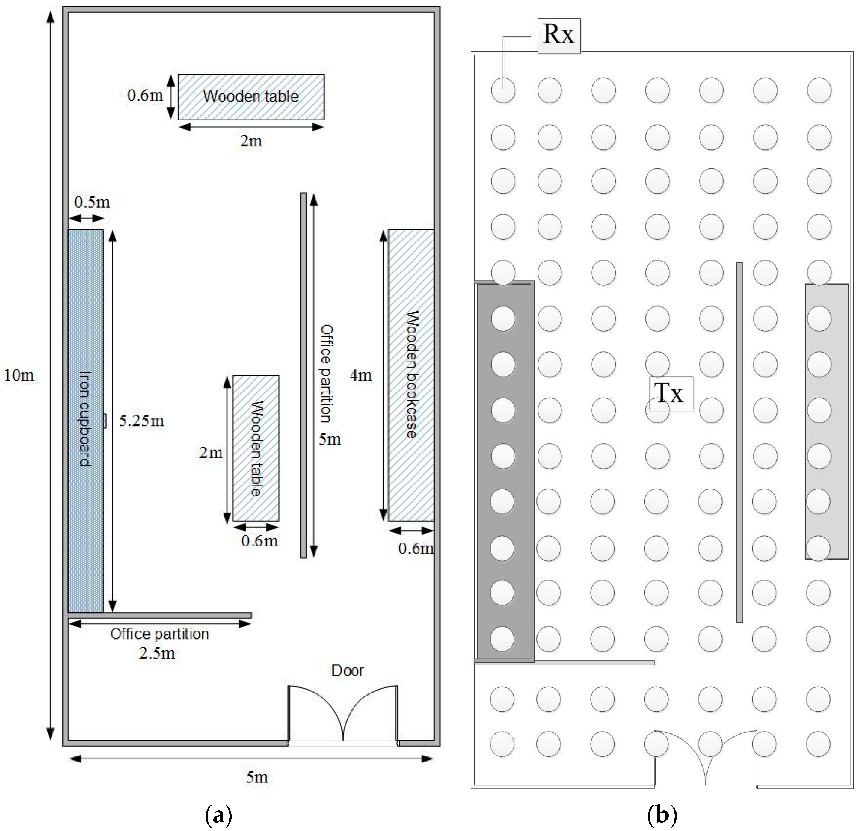
Figure 2a is the indoor environment layout, and the actual office was simulated for this paper. In this simulation, the dimension of the office was 5 m long, 10 m wide, and 4.5 m high. A partition, a wooden desk, and an iron cabinet were put inside the office. All the floors, walls, and ceilings were made of 20 cm thick concrete. The transmitter was placed at the center of the office at axis (2.5, 5.0, 2.5) m, and 105 receivers were uniformly distributed in the office, as shown in Figure 2b The height of the receivers was 1.5 m above the ground. The number of fingers for the rake receiver was 4 (NF = 4).
In a real environment, the dielectric constant and conductivity change with the frequency. Therefore, the frequency dependence for the dielectric constant and conductivity was also considered in the simulation. Since there were many receivers, the average BER and the outage probability were used for evaluating the system.
3.1. Case (A): Antenna Array
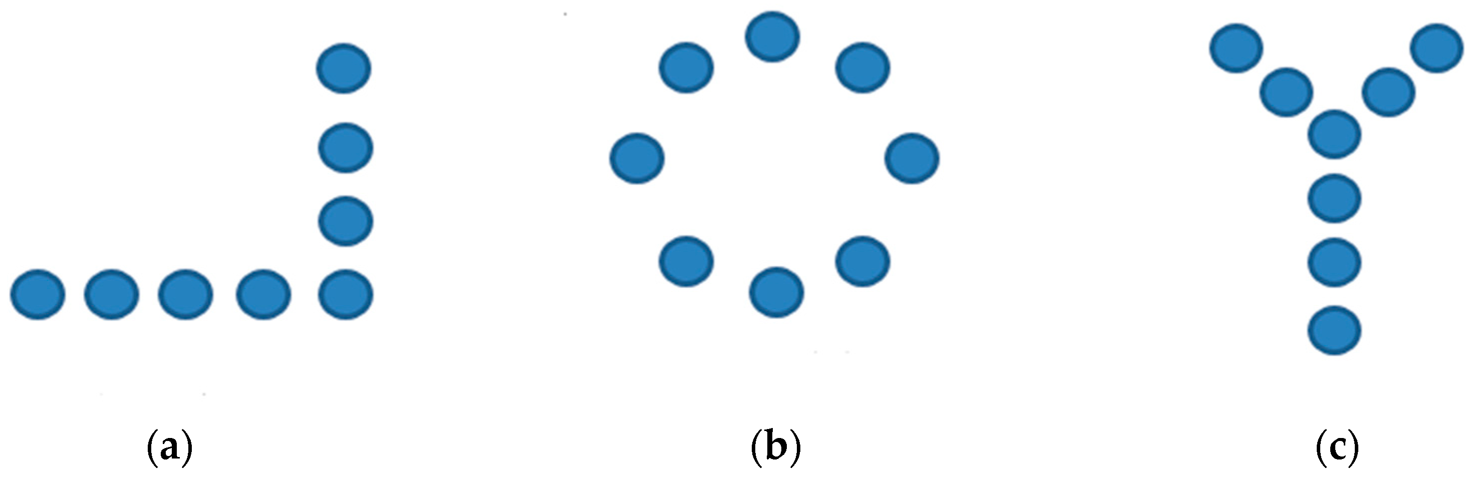
Both the transmitter and the receiver used an eight-antenna array arranged in different shapes (i.e., L-shape, circular-shape, and Y-shape), as shown in Figure 3. The transmitter was located at the center of the office at 2 m height.
The receivers were evenly distributed in the office at 1.5 m height. The performance for each shape of the antenna array in UWB frequency of 3.1–10.6 GHz was evaluated. The average BER versus SNR, the ratio of transmitting signal power to the noise power, for the 105 receivers are shown in Figure 4a, whereas the outage probability versus SNR for these receivers is shown in Figure 4b. In both figures, for most of the SNR values, the circular array has the smallest average BER and outage probability. For example, in Figure 4a, when the SNR is 68 dB, the BER values for the circular array, the L array, and the Y array are 0.18%, 0.61%, and 0.87%, respectively. In Figure 4b, when the SNR is 68 dB, the outage probability values for the circular array, the L array, and the Y array are 0.95%, 1.90%, and 1.90%, respectively. It is clear that the BER and the outage probability of the circular-shape array are better than those of the other two arrays in most of the circumstances.
3.2. Case (B): Optimal Location by Evolution Algorithm
Case (B) used SADDE and APSO to find the optimal transmitter location. To save computing time, both the transmitter and the receiver used an array of two antennas. The height of the transmitter was 2 m, and that of the receiver was 1.5 m. The outage probability was calculated as defined in Equation (7).
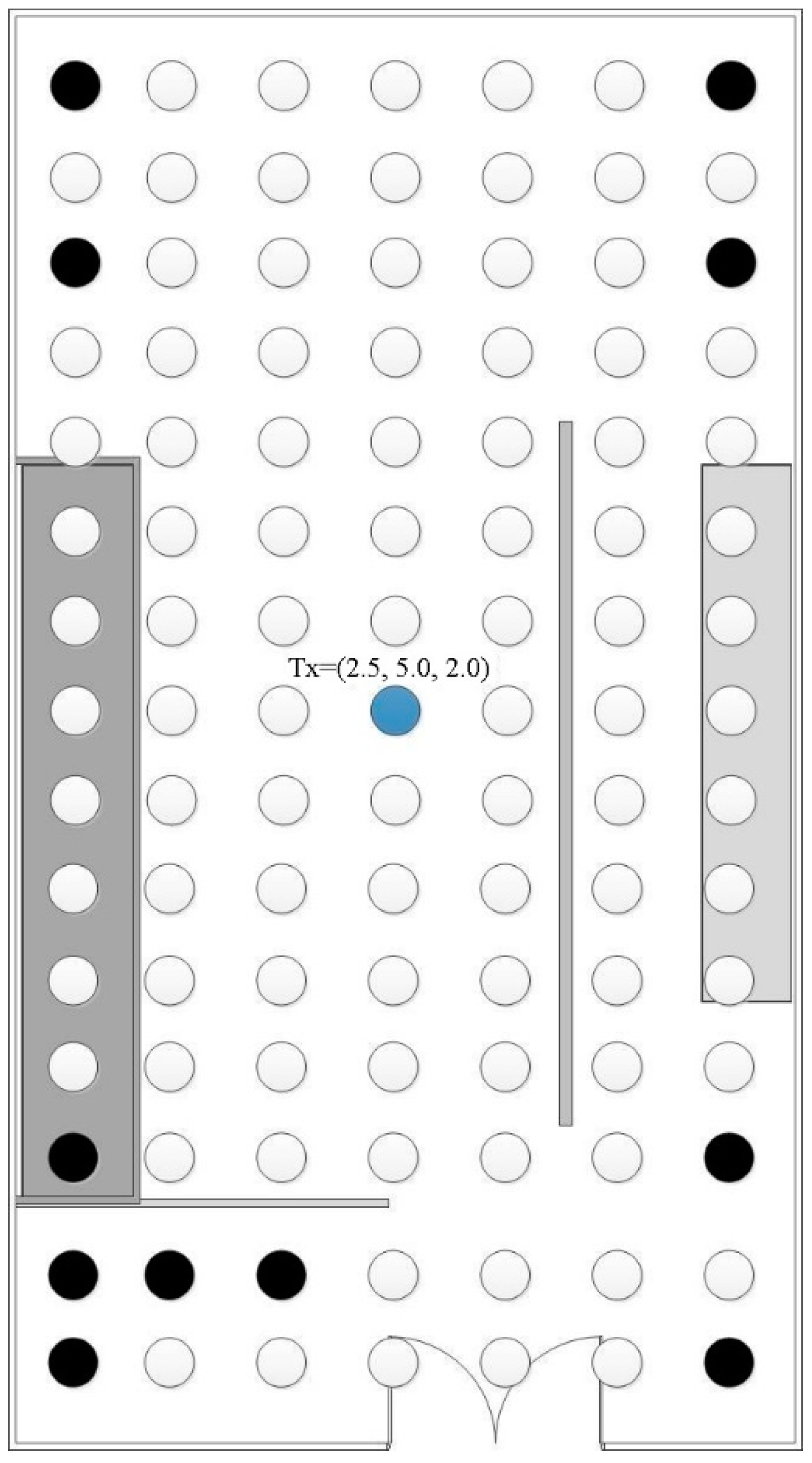
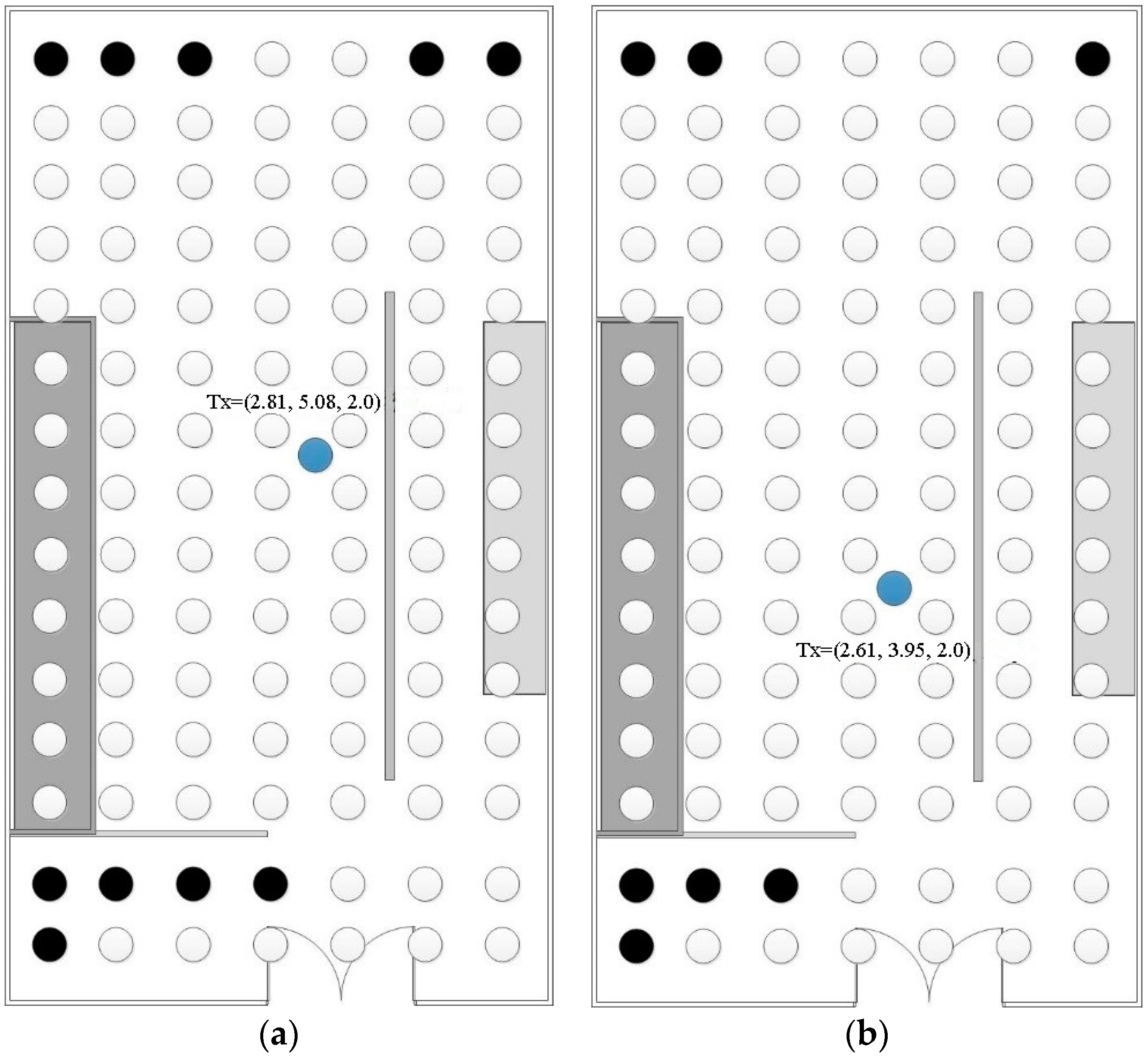
Initially, the optimal transmitter location was set at axis (2.5, 5.0, 2.0) m, the center of the office. The parameter values are shown in Table 1. As shown in Figure 5, when the SNR was 56 dB, there were 11 outage points. To improve the communication quality and reduce the outage probability [26], SADDE and APSO were used to find the optimal location of the transmitter. In Figure 6a, after using the SADDE to adjust the optimal transmitter location to axis (2.81, 5.08, 2.0) m, the outage points dropped from 11 to 10. After using the APSO to adjust the optimal transmitter location to axis (2.61, 3.95, 2.0) m, the outage points dropped from 11 to 7, as shown in Figure 6b. When the SNR increases from 56 dB to 64 dB, the number of the outage points for SADDE was reduced from 10 to 1, whereas the number for APSO dropped from 7 to 0. This result demonstrated that APSO was better than SADDE in finding an optimal transmitter location, as shown in Table 2.
4. Conclusions
For this paper, the authors applied an ROD in an MIMO-UWB system to achieve low BER and to reduce cost. Moreover, a rake receiver was used to increase the strength of the received signals to minimize the multipath effect. Three different shapes of antenna arrays, namely L-shape, circular-shape, and Y-shape, were used for both the transmitter and the receiver, and the BER performance and outage probability of each shape of the antenna array were compared. The BER and the outage probability of the circular array were better than those of the other two arrays. Two-antenna element arrays were used for the transmitter and receiver, and asynchronous particle swarm optimization (APSO) and self-adaptive dynamic differential evolution (SADDE) were used to find the optimal location of the transmitter. The results showed that APSO performs better than SADDE.
Author Contributions
W.C. initiated the idea and led the project. C.-C.C. and C.-Y.Y. conceived and designed the experiments. P.-H.H. performed the experiments. W.C. and C.-C.C. analyzed the data. C.-Y.Y. and C.-C.C. wrote the manuscript. All authors have read and approved the final version of the manuscript.
Funding
This research received no external funding.
Conflicts of Interest
The authors declare no conflicts of interest.
References
- Migliore, M.D.; Pinchera, D.; Massa, A.; Azaro, R.; Schettino, F.; Lizzi, L. An Investigation on UWB-MIMO Communication Systems Based on an Experimental Channel Characterization. IEEE Trans. Antennas Propag. 2008, 56, 3081–3083. [Google Scholar] [CrossRef] [Green Version]
- Chen, C.-H.; Liu, C.-L.; Chiu, C.-C.; Hu, T.-M. Ultra-wide Band Channel Calculation by SBR/Image Techniques for Indoor Communication. J. Electromagn. Waves Appl. 2006, 20, 41–51. [Google Scholar] [CrossRef]
- Alavi, B.; Alsindi, N.; Pahlavan, K. UWB channel measurements for accurate indoor localization. In Proceedings of the 2006 IEEE Military Communications Conference (MILCOM), Washington, DC, USA, 23–25 October 2006; pp. 1–7. [Google Scholar] [CrossRef]
- Demir, U.; Bas, C.U.; Ergen, S.C. Engine compartment UWB channel model for intra-vehicular wireless sensor networks. IEEE Trans. Veh. Technol. 2014, 63, 2497–2505. [Google Scholar] [CrossRef]
- Bas, C.U.; Ergen, S.C. Ultra-wideband channel model for intra-vehicular wireless sensor networks beneath the chassis: From statistical model to simulations. IEEE Trans. Veh. Technol. 2013, 62, 14–25. [Google Scholar] [CrossRef]
- Sadi, Y.; Ergen, S.C. Optimal power control, rate adaptation, and scheduling for UWB-based intravehicular wireless sensor networks. IEEE Trans. Veh. Technol. 2013, 62, 219–234. [Google Scholar] [CrossRef]
- Chiu, C.C.; Yu, C.Y.; Liao, S.H.; Wu, M.K. Channel capacity of multiple-input multiple-output systems for optimal antenna spacing by particle swarm optimizer. Wirel. Pers. Commun. 2013, 69, 1865–1876. [Google Scholar] [CrossRef]
- Asif, H.M.; Honary, B.; Ahmed, H. Multiple-input multiple-output ultra-wide band channel modelling method based on ray tracing. IET Commun. 2012, 6, 1195–1204. [Google Scholar] [CrossRef]
- Boche, H.; Bourdoux, A.; Fonollosa, J.R.; Kaiser, T.; Molisch, A.; Utschick, W. Antennas: State of the art. IEEE Veh. Technol. Mag. 2006, 1, 8–17. [Google Scholar] [CrossRef]
- Paulraj, A.J.; Gore, D.A.; Nabar, R.U.; Bolcskei, H. An overview of MIMO communications—A key to gigabit wireless. Proc. IEEE 2004, 92, 198–218. [Google Scholar] [CrossRef]
- He, S.; Huang, Y.; Yang, L.; Ottersten, B.; Hong, W. Energy Efficient Coordinated Beamforming for Multicell System: Duality-Based Algorithm Design and Massive MIMO Transition. IEEE Trans. Commun. 2015, 63, 4920–4935. [Google Scholar] [CrossRef]
- Zhu, D.; Choi, J.; Heath, R.W. Two-dimensional AoD and AoA acquisition for wideband millimeter-wave systems with dual-polarized MIMO. IEEE Trans. Wirel. Commun. 2017, 16, 7890–7905. [Google Scholar] [CrossRef]
- Rappaport, T.S.; Heath, R.W., Jr.; Daniels, R.C.; Murdock, J.N. Millimeter Wave Wireless Communications, 1st ed.; Prentice Hall: Upper Saddle River, NJ, USA, 2014; ISBN 978-0132172288. [Google Scholar]
- Chang, W.-J.; Tarng, J.-H.; Peng, S.-Y. Frequency-Space-Polarization on UWB MIMO Performance for Body Area Network Applications. IEEE Antennas Wirel. Propag. Lett. 2008, 7, 577–580. [Google Scholar] [CrossRef]
- Xin, Y.; Lin, Q.; Zheng, D. The BER Performance of MB-IR-UWB System Based on MIMO. In Proceedings of the 2014 3rd Asia-Pacific Conference on Antennas and Propagation, Harbin, China, 26–29 July 2014; pp. 1384–1388. [Google Scholar]
- Rahman, M.; Ko, D.-S.; Park, J.-D. A Compact Multiple Notched Ultra-Wide Band Antenna with an Analysis of the CSRR-TO-CSRR Coupling for Portable UWB Applications. Sensors 2017, 17, 2174. [Google Scholar] [CrossRef] [PubMed]
- D’Amico, A.A. Code-Multiplexing-Based One-Way Detect-and-Forward Relaying Schemes for Multiuser UWB MIMO Systems. IEEE Trans. Veh. Technol. 2017, 66, 4859–4873. [Google Scholar] [CrossRef]
- Rahman, M.; Khan, W.T.; Imran, M. Penta-notched UWB antenna with sharp frequency edge selectivity using combination of SRR, CSRR, and DGS. AEU-Int. J. Electron. Commun. 2018, 93, 116–122. [Google Scholar] [CrossRef]
- Tsao, G.H.S. Performance Characterisation of MIMO-UWB Systems for Indoor Environments. Ph.D. Thesis, University of Strathclyde, Glasgow, UK, 2014. [Google Scholar]
- Tarokh, V.; Jafarkhani, H.; Calderbank, A.R. Space-time block codes from orthogonal designs. IEEE Trans. Inf. Theory 1999, 45, 1456–1467. [Google Scholar] [CrossRef] [Green Version]
- Alamouti, S.M. A simple transmit diversity technique for wireless communications. IEEE J. Sel. Areas Commun. 1998, 16, 1451–1458. [Google Scholar] [CrossRef] [Green Version]
- Minoli, D.; Fried, S. Transmission Techniques for Emergent Multicast and Broadcast Systems; Auerbach Publications: New York, NY, USA, 2010; ISBN 9781439840665. [Google Scholar]
- Oppermann, I.; Hamalainen, M.; Iinatti, J. UWB Theory and Application; John Wiley & Sons: Hoboken, NJ, USA, 2004; ISBN 0470869178. [Google Scholar]
- Kaiser, T.; Zheng, F. Ultra Wideband Systems with MIMO; Wiley: Hoboken, NJ, USA, 2010; ISBN 9780470740002. [Google Scholar]
- Ho, M.-H.; Liao, S.-H.; Chiu, C.-C. UWB Communication Characteristics for Different Distribution of People and Various Materials of Walls. Tamkang J. Sci. Eng. 2010, 13, 315–326. [Google Scholar]
- Sun, C.-H.; Chiu, C.-C. Inverse scattering of dielectric cylindrical target using dynamic differential evolution and self-adaptive dynamic differential evolution. Int. J. RF Microw. Comput. Eng. 2013, 23, 579–585. [Google Scholar] [CrossRef]
- Lee, W.-T.; Sun, C.-H.; Chiu, C.-C.; Li, J.-F. Nondestructive Evaluation of Buried Dielectric Cylinders by Asynchronous Particle Swarm Optimization. J. Test. Eval. 2015, 43, 212–220. [Google Scholar] [CrossRef]
- Brest, J.; Greiner, S.; Boskovic, B.; Mernik, M.; Zumer, V. Self-adapting control parameters in differential evolution: A comparative study on numerical benchmark problems. IEEE Trans. Evol. Comput. 2006, 10, 646–657. [Google Scholar] [CrossRef]
- Ko, J.; Cho, Y.J.; Hur, S.; Kim, T.; Park, J.; Molisch, A.F.; Haneda, K.; Peter, M.; Park, D.J.; Cho, D.H. Millimeter-Wave Channel Measurements and Analysis for Statistical Spatial Channel Model in In-Building and Urban Environments at 28 GHz. IEEE Trans. Wirel. Commun. 2017, 16, 5853–5868. [Google Scholar] [CrossRef]
- Chalise, B.K.; Suraweera, H.A.; Zheng, G.; Karagiannidis, G.K. Beamforming Optimization for Full-Duplex Wireless-Powered MIMO Systems. IEEE Trans. Commun. 2017, 65, 3750–3764. [Google Scholar] [CrossRef]
- Ahmadi-Shokouh, J.; Tavakoli, S.; Talepour, Z. Optimality of transmitter location in a wireless network with RAKE receivers. IET Commun. 2012, 6, 3059–3064. [Google Scholar] [CrossRef]
- Cassioli, D.; Win, M.Z.; Vatalaro, F.; Molisch, A.F. Low complexity Rake receivers in ultra-wideband channels. IEEE Trans. Wirel. Commun. 2007, 6, 1265–1274. [Google Scholar] [CrossRef]
- Mielczarek, B.; Wessman, M.O.; Svensson, A. Performance of coherent UWB Rake receivers with channel estimators. In Proceedings of the 2003 IEEE 58th Vehicular Technology Conference, VTC 2003-Fall (IEEE Cat. No. 03CH37484), Orlando, FL, USA, 6–9 October 2003; Volume 3, pp. 1880–1884. [Google Scholar] [CrossRef]
- Liao, S.-H.; Chiu, C.-C.; Ho, M.-H.; Lin, C.H. Optimal Relay Antenna Location in Indoor Environment Using Particle Swarm Optimizer and Genetic Algorithm. Wirel. Pers. Commun. 2012, 62, 599–615. [Google Scholar] [CrossRef]
- Goudos, S.K.; Siakavara, K.; Samaras, T.; Vafiadis, E.E.; Sahalos, J.N. Self-adaptive differential evolution applied to real-valued antenna and microwave design problems. IEEE Trans. Antennas Propag. 2011, 59, 1286–1298. [Google Scholar] [CrossRef]
- Clerc, M. The swarm and the queen: Towards a deterministic and adaptive particle swarm optimization. In Proceedings of the 1999 Congress on Evolutionary Computation-CEC99 (Cat. No. 99TH8406), Washington, DC, USA, 6–9 July 1999; Volume 3, pp. 1951–1957. [Google Scholar] [CrossRef]
Figure 1.
System block diagram.

Figure 2.
(a) The simulated environment (top view); (b) The location of transmitting and receiving points in the simulated environment.
Figure 2.
(a) The simulated environment (top view); (b) The location of transmitting and receiving points in the simulated environment.

Figure 3.
Three different shapes of arrays for the transmitter and receiver. (a) L array; (b) circular array; (c) Y array.
Figure 3.
Three different shapes of arrays for the transmitter and receiver. (a) L array; (b) circular array; (c) Y array.

Figure 4.
(a) Average bit error rate (BER) vs. signal-to-noise ratio (SNR) for three different antenna arrays; (b) Outage probability vs. SNR for three different antenna arrays.
Figure 4.
(a) Average bit error rate (BER) vs. signal-to-noise ratio (SNR) for three different antenna arrays; (b) Outage probability vs. SNR for three different antenna arrays.
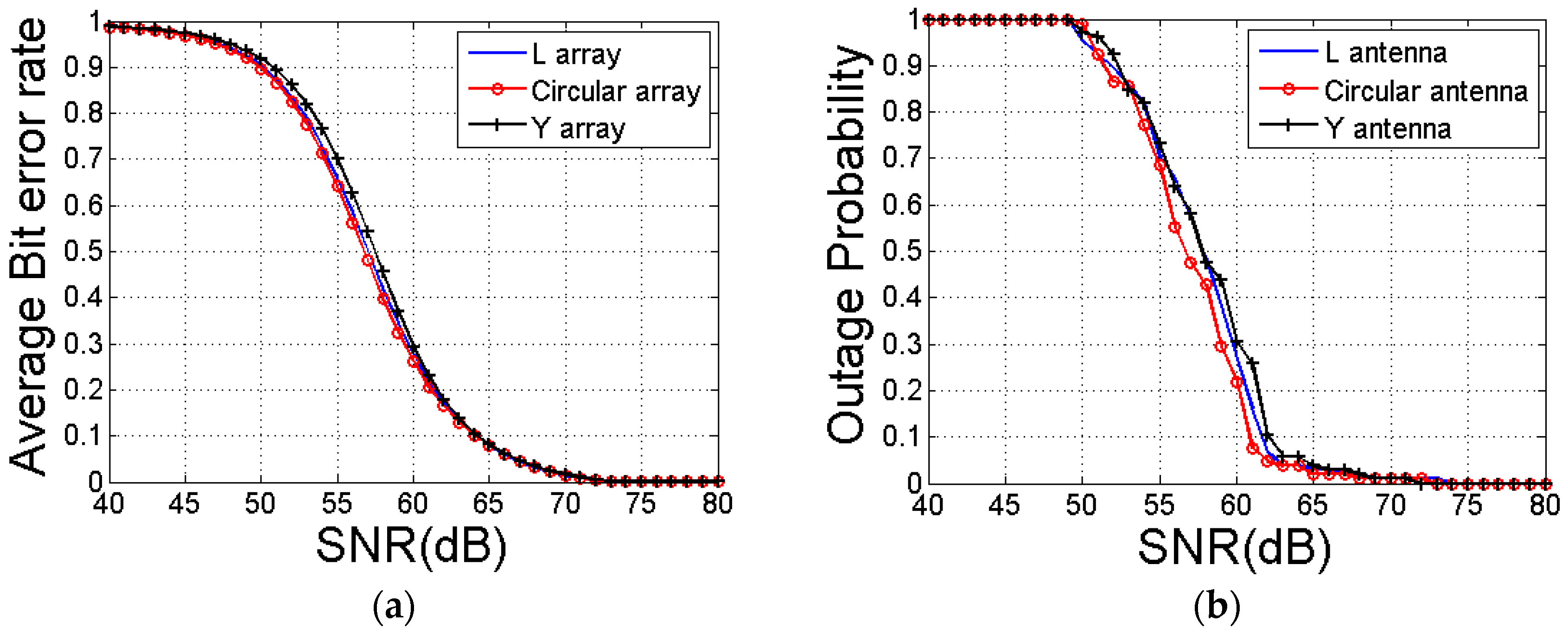
Figure 5.
The distribution of the outage points for the transmitter at (2.5, 5.0, 2.0) m. (SNR = 56 dB).
Figure 5.
The distribution of the outage points for the transmitter at (2.5, 5.0, 2.0) m. (SNR = 56 dB).

Figure 6.
(a) The distribution of the outage points for the transmitter at (2.81, 5.08, 2.0) m by self-adaptive dynamic differential evolution (SADDE); (b) The distribution of the outage points for the transmitter at (2.61, 3.95, 2.0) m by asynchronous particle swarm optimization (APSO).
Figure 6.
(a) The distribution of the outage points for the transmitter at (2.81, 5.08, 2.0) m by self-adaptive dynamic differential evolution (SADDE); (b) The distribution of the outage points for the transmitter at (2.61, 3.95, 2.0) m by asynchronous particle swarm optimization (APSO).


Table 1.
Simulation setup.
| Parameter | Value |
|---|---|
| search target (m) = (x, y, z) | location of the transmitter (x, y, 2.0) |
| fitness function | outage probability of the receivers |
| frequency range | 3.1–10.6 GHz |
| SNR | 40 dB to 80 dB |
Table 2.
Performance comparison for SADDE and APSO.
| Algorithm | SADDE | APSO | |
|---|---|---|---|
| SNR | |||
| SNR = 56 dB | Number of outage points = 10 | Number of outage points = 7 | |
| SNR = 70 dB | Number of outage points = 1 | Number of outage points = 0 | |
© 2018 by the authors. Licensee MDPI, Basel, Switzerland. This article is an open access article distributed under the terms and conditions of the Creative Commons Attribution (CC BY) license (http://creativecommons.org/licenses/by/4.0/).
Share and Cite
MDPI and ACS Style
Chien, W.; Yu, C.-Y.; Chiu, C.-C.; Huang, P.-H. Optimal Location of the Access Points for MIMO-UWB Systems. Appl. Sci. 2018, 8, 1509. https://doi.org/10.3390/app8091509
AMA Style
Chien W, Yu C-Y, Chiu C-C, Huang P-H. Optimal Location of the Access Points for MIMO-UWB Systems. Applied Sciences. 2018; 8(9):1509. https://doi.org/10.3390/app8091509
Chicago/Turabian StyleChien, Wei, Chia-Ying Yu, Chien-Ching Chiu, and Po-Hsuan Huang. 2018. "Optimal Location of the Access Points for MIMO-UWB Systems" Applied Sciences 8, no. 9: 1509. https://doi.org/10.3390/app8091509
Note that from the first issue of 2016, this journal uses article numbers instead of page numbers. See further details here.