Multi-Objective Virtual Power Plant Construction Model Based on Decision Area Division

Abstract

Virtual power plant (VPP) is an effective technology form to aggregate the distributed energy resources (DERs), which include distributed generation (DG), energy storage (ES) and demand response (DR). The establishment of a unified and coordinated control of VPP is an important means to achieve the interconnection of energy internet. Therefore, this paper focuses on the research of VPP construction model. Firstly, a preliminary introduction on all kinds of the DERs is carried out. According to the relevant guidelines, the decision area of the VPP is carefully divided, and the decision variables representing the various resources in the area are determined. Then, in order to get a VPP with low daily average cost, good load characteristics, high degree of DG consumption and high degree of resource aggregation, a multi-objective VPP construction model based on decision area division is established, and various constraints including geographic information are considered. The improved bat algorithm based on priority selection is used to solve this model. Finally, the correctness and effectiveness of the model are verified by an example.

1. Introduction

With the increasing demand for electricity and the increasingly severe problems of energy shortage and environmental pollution in the world, the disadvantages of traditional energy generation are becoming more and more prominent [1]. As a result, countries around the world have introduced policies to encourage companies to optimize their energy structure, promote energy conservation and emission reduction, and achieve sustainable economic development. In this new situation, the distributed energy resources (DERs) have been vigorously developed. These DERs have the characteristics of environmental protection and low energy consumption, and small investment can also improve the flexibility of the power system [2,3]. However, single DER is difficult to directly participate in market transactions, so aggregation technology is widely used. To this end, virtual power plant (VPP), microgrids and load aggregators (LAs) have been developed one after another. The microgrid takes the distributed generation (DG) and user as the main control targets, but it is restricted by geographical areas [4]. The VPP can reduce the geographical restrictions of DG aggregation and aggregate various DERs. Either microgrids or VPPs are more widely used in the generation side, focusing more on the integration of DERs and optimal scheduling. The LA is a resource aggregator with external load characteristic and strong responsive capability [5]. Therefore, this paper mainly studies the VPP.

In order to achieve effective management of DERs with large quantities and scattered geographical locations, and eliminate the intermittent and random effects of renewable energy power generation, the concept of VPP has been mentioned [6,7,8]. The VPP can aggregate DERs based on their respective characteristics, achieve efficient use of various types of resources, and reduce the generation of abandoned wind power (WP) and photovoltaic (PV). The VPP has developed rapidly in recent years, such as Vattenfall and Next Kraftwerke in Germany [9]. In China, a VPP demonstration project has come into use in Yunnan Province [10]. Moreover, the VPPs constructed in different regions have different characteristics, so the actual geographic information should be taken into account when constructing VPPs. From a microscopic perspective, the VPP can be considered as the integration and coordination optimization of DERs through advanced information and communication technologies and software systems. The VPP is a power coordination management system that participates in the power market and grid operation as a special power plant [11]. Therefore, how to select various DERs for the construction of VPP is a prerequisite for the efficient use of resources, and it has important research significance.

In the reasonable selection of DERs for aggregation and construction of VPPs, it is necessary to research the characteristics and correlation of various DERs. Many scholars have achieved research results. In Reference [12], the VPP components are introduced, including the wind power plants (WPPs), PVs, conventional gas turbines (CGTs), energy storage systems (ESSs) and demand resource providers (DRPs). In Reference [13], the conditional value at risk (CVaR) and confidence degree theory are introduced to build models for VPP connections with the WPP, PV, CGT, ESSs and incentive-based demand response (IBDR). In Reference [14], the implementation costs of demand response (DR) has been firstly taken into account, and then WPPs, PV, electric vehicles and conventional power plants have also been researched.

The VPP is selective to select DERs for aggregation and there are different methodological guidelines in the aggregation process. In Reference [12], a two-tier robust scheduling model is established. The upper layer uses the VPP operating revenue as the maximum objective function, and the lower layer uses the minimum system payload and operating cost as objective functions. In Reference [15], using the minimum operating cost of 24-h VPP as the objective function, the teaching–learning based optimization (TLBO) heuristic algorithm is proposed to solve the model. In Reference [16], after considering the electric boiler in the VPP operation mode of the integrated thermoelectric system, a multi-objective model is established, including the carbon emission cost, the total operating cost of VPP, and the transaction electricity between the VPP and the main transaction power. In Reference [17], a mixed-integer linear programming model is proposed, which targets the maximum weekly profit of VPP and is subject to long-term bilateral contracts and technical conditions. In Reference [18], the actual location and specific functions of each DER in the public network can be considered, and a large-scale VPP optimization model has been established. In Reference [19], the technical VPP (TVPP) takes into account the real-time influence of the local network on the DER-aggregated profile. In Reference [20], for EES units with integer constraints, a mixed integer linear programming (MILP) algorithm, which takes into account the grid constraints, is proposed.

Based on the above-mentioned references, the research on the related scheduling of VPP is more mature. However, there are few studies on how to construct VPPs. The disadvantages and deficiencies of the aforementioned references are as follows: the types of involved DERs are few, the differences between different types of DERs in different functional areas are less considered, the complementarity between various DERs is less considered, and the proposed construction indicators are also relatively single. In addition, the geographical information and resource characteristics are rarely combined to consider. Combined with the existing research results and shortcomings in the references, the contributions of this paper are as follows: (1) the idea of decision area division for determining decision variables is proposed. (2) A multi-objective VPP construction model with low daily average costs, fine load characteristics, a high degree of DG consumption and a high degree of resource aggregation is established. (3) The complementary constraints between various DERs have been considered and a fusion space distance that accounts for geographical information and load density has also been introduced. (4) The improved bat algorithm based on the preference degree is used to solve the multi-objective 0–1 programming model.

Therefore, the purpose of this paper is to propose a reasonable plan for selecting distributed generation (DG), energy storage (ES) and demand response (DR). The rest of this paper is organized as follows: in Section 1, some kinds of DERs are introduced, the decision area according to the relevant criterion is divided and then the decision variables are also determined. In Section 2, a multi-objective VPP construction model based on decision area division is established and various constraints including geographic information are also considered. In Section 3, an improved bat algorithm based on the preference degree, which is to solve this multi-objective 0–1 programming model, is introduced. In Section 4, the example analysis are conducted. In Section 5, summary and relevant analysis are given.

2. Decision Area Division and Decision Variable Determination of Virtual Power Plant

2.1. Distributed Energy Resource Output Model

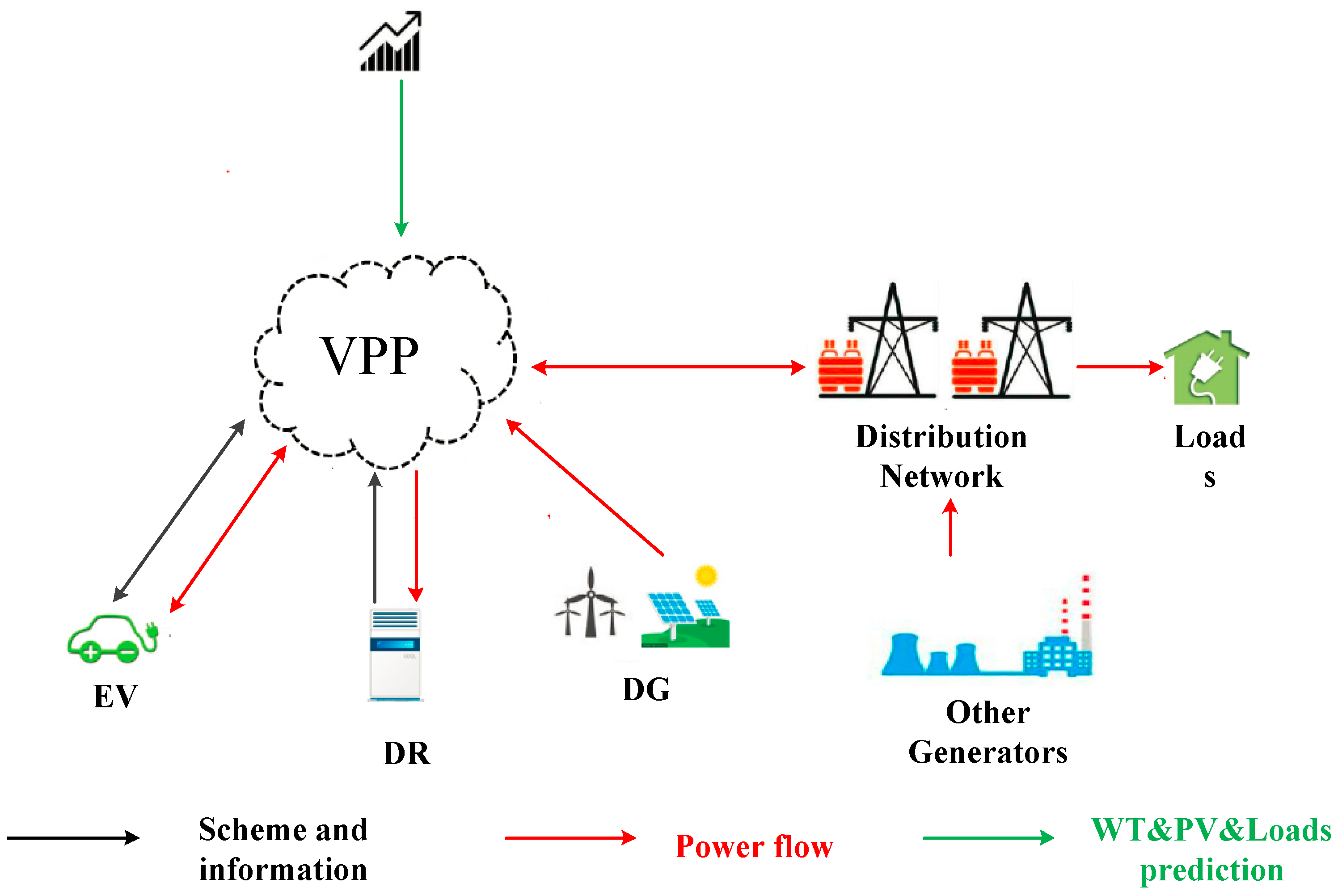
The distributed DERs of a certain area constitute a VPP; therefore, the whole VPP is not restricted by the geographical area, and the control mode can be decentralized or centralized. The VPP is proposed to integrate all kinds of DER, including the DG, ES and DR, which is shown in Figure 1.

By referring to the relevant references, most of authors take the DERs widely distributed in the city as research objectives in the study of VPP, such as the WP, PV, ES and flexible load [12,13,14,21]. First of all, the mathematical model of these DERs is briefly introduced according to the relevant references.

1. Wind power Generation Model

The output of WP is mainly affected by the wind speed and direction, and the wind speed and direction of different fans can be the same as those in the same power plant. Therefore, the output power P_t of a single fan is obtained according to the power characteristic curve of the wind turbine, the product of the sum of all the fan power and the coefficient representing the output power [13], and can be described as:

$$P_t=\{\begin{array}{c}0\\ A+B\times S{W}_t+C\times S{W}_t^2\\ P_r\\ 0\end{array}\begin{array}{c}0\le S{W}_t\le V_{ci}\\ V_{ci}\le S{W}_t\le V_r\\ V_r\le S{W}_t\le V_{co}\\ V_{co}\le S{W}_t\end{array}$$

(1)

where $A=\frac{1}{{(V_{ci}-V_r)}^2}\left[V_{ci}(V_{ci}+V_r)-4(V_{ci}{V}_r){\left(\frac{V_{ci}+V_r}{2V_r}\right)}^3\right]$, $B=\frac{1}{{(V_{ci}-V_r)}^2}\left[4(V_{ci}+V_r){\left(\frac{V_{ci}+V_r}{2V_r}\right)}^3-3(V_{ci}+V_r)\right]$, $C=\frac{1}{{(V_{ci}-V_r)}^2}\left[2-4{\left(\frac{V_{ci}+V_r}{2V_r}\right)}^3\right]$, SW_t is the wind speed at the location of the fan, V_ci is the threshold wind velocity of the fan, V_r is the rated wind speed of the fan, V_co is the resection wind speed of the fan, and P_r is the rated power of the fan.

2. Photovoltaic Generation Model

The PV generation system is mainly constituted by power generation and conversion systems, which is composed of PV panels, controllers, ESs and conversion devices. The output power of PV generation system is directly related to the light intensity, and its power output model is [14]:

$$P_{PV}=\{\begin{array}{c}{P}_{sn}{R}^2/R_r{R}_c\\ P_{sn}R/R_r\\ P_{sn}\end{array}\begin{array}{c}0\le R<R_c\\ R_c\le R<R_r\\ R\ge R_r\end{array}$$

(2)

where P_PV is the actual output power of PV generation system, P_sn is the rated power of the PV generation system, R_c is the characteristic intensity of solar irradiance which is generally 150 W/m², and R_r is the solar radiation intensity when the PV power generation system just reaches the rated power (generally 1000 W/m²).

3. Energy Storage Model

ES technologies can be classified into mechanical ES, electrical ES, electrochemical ES, thermal ES, and chemical ES, according to the different storage media. As an application form of ES, electric vehicles have the characteristics of flexible regulation and widely exist on the user side. Therefore, the ES devices in this paper mainly consider electric vehicles. The main factors affecting the charging curve of electric vehicles include the quantity, type, charging characteristics and user behavior of electric vehicles [22]. The initial charge state of a single electric vehicle battery is related to mileage, which is shown as follows:

$$SO{C}_0=1-D/L$$

(3)

where SOC₀ is the initial charging state, D is the actual mileage number, and L is the maximum mileage number.

According to the initial charge state of electric vehicle battery, the charging duration time and charging power of single vehicle can be obtained, and then the daily charging curve of all the electric vehicles can be obtained. Taking Toyota RAV4 electric vehicle as an example. According to the charging characteristics of a typical battery, the charging power of an electric vehicle can be calculated and expressed by a piecewise function [23]:

$$P=\{\begin{array}{c}3.65+9.15SOC\\ 5.48\\ 5.48+4.55(SOC-0.8)\end{array}\begin{array}{c}0\le SOC<0.2\\ 0.2\le SOC<0.8\\ 0.8\le SOC<1.0\end{array}$$

(4)

where P is the charging power and the unit is kW, SOC is the state of charge.

4. Flexible Load Model

From the user perspective, flexible loads can be divided into transferable loads, interruptible loads, and translational loads [24]. The transferable load is to maintain the power consumption within a certain period of time, but the power consumption can be flexibly adjusted at each time. It can reduce the power consumption during the peak period and increase the power consumption during the low period. The interruptible load can be responded to the demand side according to the demand for electricity. Generally, it has instantaneous power-off characteristics, but it does not require ES characteristics. The working time and power demand are flexible and controllable. The translational load is constrained by the production process and can only translate the power curve at different time periods, which is embodied in the overall transfer of the electric power curve [25]. Based on the electricity price response, the flexible load can be described as:

$$\Delta P_{shift}(k)=g_1(P_0(k),\Delta p_{shift}(k),k_{shift}(k),v_{shift}(k))$$

(5)

$${\displaystyle \sum _{k=1}^T\Delta P_{shift}(k)=0}$$

(6)

where ΔP_shift(k) is the response amount of the transferable load at period k, P₀(k) is the base load at period k, Δp_shift(k) is the power price difference between period k and other periods, k_shift(k) is the mutual elasticity between period k and other periods, v_shift(k) is the transfer rate, T is the time period.

The response amount of interruptible load within a certain period can be written as:

$$\Delta P_{re}(k)=g_3(P_0(k),\Delta p_{re}(k),l_{re}(k),v_{re}(k))$$

(7)

where Δp_re(k) is the change in price of period k, l_re(k) is the elastic coefficient of the period k, and v_re(k) is cutting speed.

The response amount of translatable load can be described as:

$$\Delta P_{shape}(k)=g_2(k+\Delta k(\Delta p))-g_2(k)$$

(8)

where g₂(t) is the initial power consumption curve, and Δk(Δp) is the load translation period caused by Δp.

2.2. Division of Decision Area

In order to reduce the number of decision variables, we first divide the decision area of VPP, that is, according to some criteria, a region can be divided into several blocks. At this time, the numbers of decision variables are changed from the numbers of distributed power, controllable load and ES device before the division area to the numbers of distributed power, controllable load and ES device in the region.

The main basis for determining the decision area of VPP is: regional load density, power consumption levels, administrative ranks, economic levels and user importance [26]. Then, we can choose whether to formulate appropriate service agreements for each area and participate in the construction of VPP. In this paper, the decision areas of VPP are divided according to the regional function, mixed resource power and regional area.

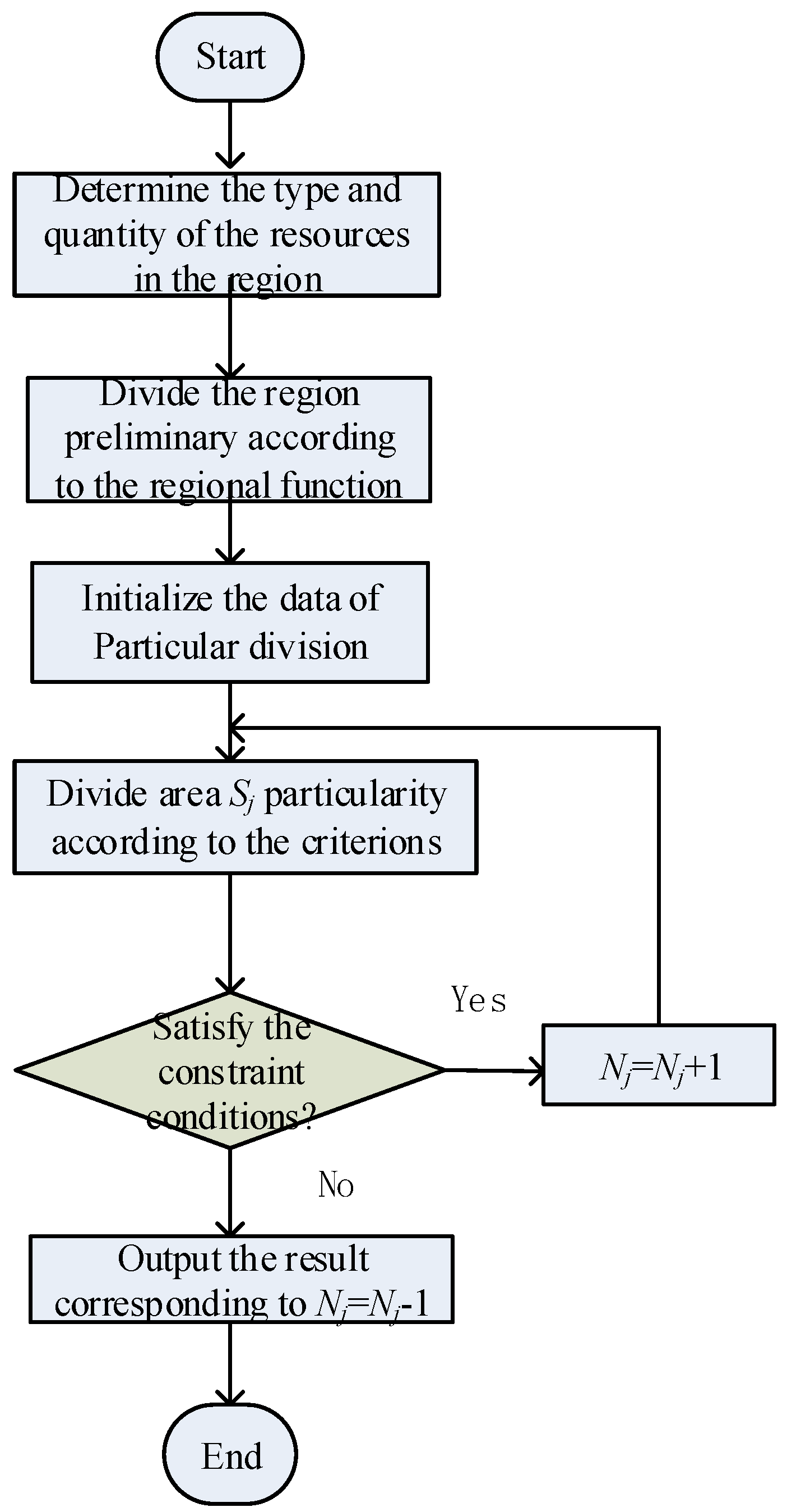
According to the different functions of urban areas, they can be divided into residence, industry, commercial finance, administrative office, culture and entertainment, medical and health, education and scientific research, municipal facilities, warehousing, transportation and agriculture. Mixed resources include the DG, ES and controllable load, and the mixed resource power is the sum of these three resources. According to the regional function, the region is divided into K blocks, and the area j can be recorded as S_j (j = 1, 2, …, K). Then, each area is carefully divided. The division criterion is to minimize the number of divided areas under certain constraints, that is, the regional area cannot exceed S_maxj, and the maximum power of the mixed resource in each area cannot exceed Q_maxj. The area S_j is divided according to the regional function, so the mixture resource density ρ_j is different. There is a negative function relationship between S_maxj and ρ_j. The steps for dividing the decision area of VPP are as follows:

(1)

Determine the type and quantity of resources in different locations of the region.

(2)

Divide the region preliminary according to the regional function, and record the area as S_j (j = 1, 2, …, K).

(3)

Divide area S_j particularity, initialize division block number N_j in each area, determine the parameters S_maxj and Q_maxj in the constraints.

(4)

According to the number N_j of areas, make S_j divided into equal areas. Determine whether to meet the constraints; if satisfied, turn (5), and vice versa (6).

(5)

N_j = N_j + 1, return to (3).

(6)

Obtain the final detailed division result of regional S_j, which is the corresponding division result of N_j = N_j − 1.

The flow chart of the decision area of VPP is shown in Figure 2.

This paper illustrates the steps of the decision area division of the VPP by the following figure.

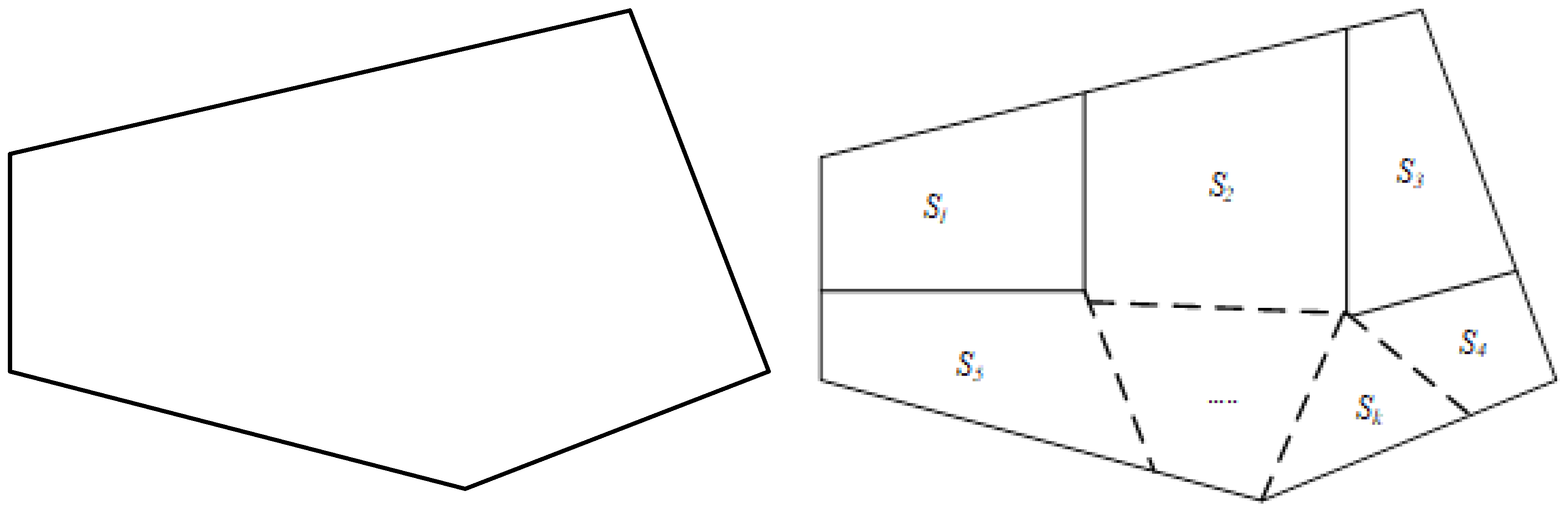
Firstly, a preliminary division is made according to the region function, which is shown in Figure 3. Then, each region is detailed divided according to the relevant criteria; for example, the area S₁ is finally divided into 4 parts, which is shown in Figure 4.

Assuming that the area S_j can be divided into C_j sub-areas, the region is divided into m areas after the detailed division, which is as follows:

$$m={\displaystyle \sum _{j=1}^K{C}_j}$$

(9)

The decision variables, which represent whether there are distributed power sources, ES devices and controllable loads in the area i (i = 1, 2, …, m), are represented by vector X_i which is made up of 0 and 1 elements and can be written as:

$$X_i={\left[X_i^{DG},X_i^{ES},X_i^{DR}\right]}^T$$

(10)

The set of decision variables in the whole region is:

$$\left(X_1,X_2,\dots ,X_{m-1},X_m\right)=\left[\begin{array}{ccccc}{X}_1^{DG}& X_2^{DG}& \dots & X_{m-1}^{DG}& X_m^{DG}\\ X_1^{ES}& X_2^{ES}& \dots & X_{m-1}^{ES}& X_m^{ES}\\ X_1^{DR}& X_2^{DR}& \dots & X_{m-1}^{DR}& X_m^{DR}\end{array}\right]$$

(11)

When modeling the construction of a VPP, the traditional method sets all resource in the large region as a decision variable, but the method of determining the decision variables by dividing the decision area greatly can reduce the numbers of decision variables and the difficulty of calculation.

3. The Construction Model of Virtual Power Plant

3.1. Objective Function

1. Minimum Daily Average Cost

The output power of the VPP at each time period is planned, and the power generation cost and charging cost are also considered. The punishment cost is used to indicate the degree of actual output deviating from the planned output, the power generation cost refers to the DG cost, and the charging cost refers to the ES cost. The objective function is:

$$\begin{array}{l}\min f_1=C^{DG}+C^{ES}+C^{SN}\\ ={\displaystyle \sum _{k=1}^n{\displaystyle \sum _{i=1}^m{C}_{ki}^{DG}{P}_{ki}^{DG}{X}_i^{DG}}}+{\displaystyle \sum _{i=1}^m{n}_i{C}_i^{ES}}{X}_i^{ES}+C_s\left|{\displaystyle \sum _{k=1}^n[{\displaystyle \sum _{i=1}^m(-P_{ki}^{DG}{X}_i^{DG}+P_{ki}^{ES}{X}_i^{ES}-P_{ki}^{DR}{X}_i^{DR})+P_{k0}]}}\right|\end{array}$$

(12)

where k is a time series, taking 1 h as a time period, k = 1, 2, …, 24; f₁ is the daily cost of VPP; C^DG is the daily average generation cost of DR; C^ES is the daily charging cost of ES device; C^SN is the punishment cost for the VPP to pay the grid; $P_{ki}^{DG}$ is the DR output of area i at time period k; $X_i^{DG}$ represents whether there is a DR generation in area i, and if satisfied, the value is 1, and vice versa 0; n_i is the daily average charging times of ES devices; $P_{ki}^{ES}$ is the charging power of ES device of area i at time period k; $X_I^{ES}$ represents whether there is a ES device in the area i, and if satisfied, the value is 1, and vice versa 0; $P_{ki}^{DR}$ is the controllable load power of area i at time period k; C_s is the unit punishment cost; and P_k0 is the planned output at time period k.

When there is a deviation between the actual output and the planned output of the VPP, the power grid needs to reserve the reservation to compensate for the deviation, which will produce the cost at this time; most of the electric power in the power grid is thermal power, so the unit punishment cost can be considered as the thermal power cost.

2. Optimal Daily Load Characteristics

If the curve L represents the difference between the actual output and the planned output of the VPP, the daily load characteristics can be measured by the volatility of the curve L. Volatility is defined as the ratio of standard deviation to geometric mean of active power. The standard deviation of the load reflects the degree of the load dispersion, the geometric mean of the load reflects the degree of the load concentration, and the ratio of the standard deviation to the geometric mean reflects the relative size of the load dispersion [27]. The objective function is:

$$\{\begin{array}{l}\min f_2=\frac{\sigma }{\mu }=\frac{\sqrt{\frac{1}{n}{\displaystyle \sum _{k=1}^n{(L_k-\overline{L})}^2}}}{\sqrt[n]{{\displaystyle \prod _{k=1}^n{L}_k}}}\\ L_k={\displaystyle \sum _{i=1}^m(-P_{ki}^{DG}{X}_i^{DG}+P_{ki}^{ES}{X}_i^{ES}-P_{ki}^{DR}{X}_i^{DR}})+P_{k0}\end{array}$$

(13)

where f₂ is the volatility of the curve L; σ is the standard deviation; μ is the geometric mean; L_k is the difference between the actual output and planned output of the VPP at time period k; and $\overline{L}$ is the arithmetic mean of output power.

The smaller the difference between the actual output and the planned output, the smoother the curve L is, the better the stability of the system is, and the easier the power grid is to be dispatched.

3. Highest Degree of Distributed Generation Consumption

One of the functions of the VPP construction is to promote the consumption of DG, reduce the abandoned wind the power rate and abandoned PV rate, and make full use of clean energy. In this paper, the optimal objective is to maximize the daily average power of DG, that is, when the power of the VPP is less than the planned power, the DG can be fully utilized. Otherwise, when the output is greater than the planned output, the DG cannot be fully utilized. The objective function is:

$$\{\begin{array}{l}\max f_3={\displaystyle \sum _{k=1}^n[a{\displaystyle \sum _{i=1}^m{P}_{k0}+(1-a){\displaystyle \sum _{i=1}^m{P}_{ki}^{DG}{X}_i^{DG}}]}}\\ a=\{\begin{array}{l}1,{\displaystyle \sum _{i=1}^m{P}_{ki}^{DG}{X}_i^{DG}-P_{ki}^{ES}{X}_i^{ES}+P_{ki}^{DR}{X}_i^{DR}-P_{k0}\ge 0}\\ 0,{\displaystyle \sum _{i=1}^m{P}_{ki}^{DG}{X}_i^{DG}-P_{ki}^{ES}{X}_i^{ES}+P_{ki}^{DR}{X}_i^{DR}-P_{k0}<0}\end{array}\end{array}$$

(14)

where a is the coefficient, which represents whether the DG is fully utilized; if satisfied, the value is 0, and vice versa. It is for 0, and vice versa 1.

Through the construction of VPP, the DG resources in the area can be utilized to the greatest extent, but if all the DG are selected to construct, these resources will cause a lot of waste, so we should make a reasonable choice to make the highest degree of DG consumption.

4. Highest Degree of Regional Polymerization

When selecting resources for every area, we need to consider the spatial location and load density of the area. The spatial location attribute and the load density attribute of each area are regarded as the attribute data of the spatial elements, and the correlation calculation of the degree of regional aggregation is carried out by using the fusion distance between the two kinds of attributes. The definition of fusion space distance is:

$$d(i,j)={\omega }_p\Vert p_i-p_j\Vert +{\omega }_{\rho }\Vert {\rho }_i-{\rho }_j\Vert$$

(15)

where ω_p and ω_ρ are the weights of spatial location and load density attributes, respectively, and the sum of them is 1; p_i and p_j are the position coordinates of area i and area j; ρ_i and ρ_j are the load densities of area i and area j, respectively.

In this paper, the degree of regional polymerization is measured by the sum of the maximum fusion space distance of m areas. The objective function is:

$$\{\begin{array}{l}\min f_4={\displaystyle \sum _{i=1}^m\max \{X_i{X}_{h}d(i,h)\}}\\ h=1,2,\dots ,m\end{array}$$

(16)

where X_i and X_h indicate whether there is any resources involved in the construction of the VPP in areas i and h, respectively, and if satisfied, the value is 1, and vice versa 0; d(i, h) represents the fusion space distance between areas i and h.

To sum up, the optimal objective function set of VPP is as follows:

$$F=(\min f_1,\min f_2,\max f_3,\min f_4)$$

(17)

The objective function F represents the minimum daily average cost, the optimal daily load characteristics, the highest degree of DG consumption and the highest degree of regional polymerization.

3.2. Constraint Condition

1. Virtual Power Plant Scale Constraint

The VPP can aggregate the DG, ES and controllable load into a whole, so that it can participate in the operation of the electricity market and the auxiliary service market, and the number of resources and the size of the power consumption scale should not be too small for the construction of the VPP, which satisfy:

$$\{\begin{array}{l}{\displaystyle \sum _{i=1}^m(X_i^{DG}+X_i^{ES}+X_i^{DR})\ge M_{\min }}\\ {\displaystyle \sum _{i=1}^m{\displaystyle \sum _{k=1}^n(P_{ki}^{ES}{X}_i^{ES}+P_{k0})}}\ge Q_{k\min }\end{array}$$

(18)

where M_min is the minimum number of resources; and Q_min is the minimum power consumption in time period k.

2. Fusion Space Distance Constraint

There is a fusion space distance between any two areas, and the fusion space distance should be controlled within a certain range, not too large, which satisfies:

$$\max d(i,j)\le d_{\max }$$

(19)

where d_max is the maximum fusion space distance.

3. Virtual Power Plant Output Constraint

The VPP output constraint can be written as:

$$P_{k\min }\le {\displaystyle \sum _{i=1}^m(P_{ki}^{DG}{X}_i^{DG}-P_{ki}^{ES}{X}_i^{ES}-P_{ki}^{DR}{X}_i^{DR})}\le P_{k\max }$$

(20)

where P_kmin and P_kmax are the minimum and maximum values of VPP output at time period k, respectively.

4. Curve Volatility Constraint

In order to make the actual output curve closer to the planned output curve and improve the operation stability of the VPP, the volatility of the curve L should not be too large, which is described as:

$$\frac{\sigma }{\mu }\le {\theta }_{\max }$$

(21)

where θ_max is the upper limit of the volatility.

5. Resource Complementarity Constraint

In order to minimize the influence of the uncertain factors on the VPP and improve the stability of the system, the complementarity among various resources should be fully considered in the construction of VPP. The measurement of resource complementarity is the measurement of the difference between different load curves in the same time period. The dissimilarity and similarity are corresponding to each other. The higher the similarity between the curves is, the lower the complementarity is, and vice versa [28]. The correlation among all kinds of resources is as follows:

$${\beta }_{xy}=\left[{\displaystyle \sum _{k=1}^n\frac{\Lambda (k)}{1+\left|\Delta x(k)/({\sigma }_k\Delta k)-\Delta y(k)/({\sigma }_k\Delta k)\right|}}\right]/\left[{\displaystyle \sum _{k=1}^n\Lambda (k)}\right]$$

(22)

where Λ(k) is the weighting function of active power at different time periods; σ_x is the standard deviation of the resource sequence x(k); and σ_y is the standard deviation of the resource sequence y(k).

The resource complementarity coefficient between resources x and y is:

$${\gamma }_{xy}=1-{\beta }_{xy}$$

(23)

In this paper, the DG, ES and controllable load are involved in the construction of VPP. Therefore, the sum of the complementarity coefficients among different resources is taken as the complementary coefficient of the whole VPP, which is recorded as γ_VPP.

In order to guarantee the complementarity among various resources, the condition should be restrained and is shown as following:

$${\gamma }_{VPP}\ge {\gamma }_{\min }$$

(24)

where γ_min is the lower limit of complementarity.

4. The Improved Bat Algorithm Based on Priority Selection

4.1. Basic Bat Algorithm

In this paper, for the multi-objective 0–1 programming model of VPP, the improved bat algorithm based on priority selection can be used to obtain the construction scheme of VPP, which satisfies the multi-objective programming.

The Bat algorithm is a new heuristic algorithm, which simulates the echolocation principle of microbats. Assuming that in a d-dimensional search space, the location of the bat i in the generation t is $x_i^t$, the speed is $v_I^t$, the pulse frequency is F_i, the current best position of bat population is x*, and the update formulas of $x_i^t$ and $v_i^t$ are as follows:

$$F_i=F_{\min }+(F_{\max }-F_{\min })\beta$$

(25)

$$v_i^t=v_i^{t-1}+(x_i^t-x^{*})f_i$$

(26)

$$x_i^t=x_i^{t-1}+v_i^t$$

(27)

The above update formula corresponds to global search. For local search, the current optimal solution x_old is selected from the known optimal solution set, and then a new location is generated near that location, which is obtained by:

$$x_{new}=x_{old}+\epsilon A^t$$

(28)

where ε is the random number between −1 and 1; and A^t is the average loudness of all bats.

In order to take account of global search and local search at the same time, we need to dynamically adjust loudness A_i and rate R_i. In general, the loudness will gradually decrease with the number of updates, and the rate will gradually increase with the number of updates, which are shown as:

$$A_i^{t+1}=\alpha A_i^t$$

(29)

$$R_i^{t+1}=R_i^o[1-\exp (-\gamma t)]$$

(30)

where α and γ are constants, i.e., 0 < α < 1, γ > 0; when t → ∞, $A_i^t$ → 0, $R_i^t$ → $R_i^o$.

4.2. Improved Bat Algorithm Based on Priority Selection

As the basic bat algorithm is used to solve the problem of function optimization in the continuous domain, it is necessary to redefine the bat position and update the speed equation to solve the 0–1 programming problem. After iterating many times, the pareto optimal solutions are finally obtained. Then, the priority selection of each bat in the pareto solution set is calculated [29], and the bat position with the largest priority selection is selected as the compromise optimal solution. First, Equations (26)–(28) are modified as:

$$v_i^{t+1}=xor(v_i^t,round(xor(x_i^t,x^{*})\times F_i))$$

(31)

$$x_i^{t+1}=or(x_i^t,v_i^{t+1})$$

(32)

$$\begin{array}{c}{x}_{i,new}(i)=or(x_{old},round(\epsilon A^t))\\ i=1,2,\dots ,n\end{array}$$

(33)

where round is the rounding operation; x_or and or refer to logical “xor operation” and “or operation”, respectively; x* is the best location for the bat population; and t is the algebra of bats.

The steps of the improved bat algorithm based on priority selection are as follows:

(1) Initialize the size of the bat population n, the location of the bat i x(i), the velocity v(i), the pulse emission speed R(i), the pulse frequency F(i), the pulse loudness A(i), and the target function f_i(x(i)), and then determine the current pareto optimal solution.

(2) Generate a new solution set x_new and update the bat’s speed and location according to Equations (34)–(36):

$$F_i=F_{\min }+(F_{\max }-F_{\min })\beta$$

(34)

$$v_i^{t+1}=xor(v_i^t,round(xor(x_i^t,x^{*})\times F_i))$$

(35)

$$x_i^{t+1}=or(x_i^t,v_i^{t+1})$$

(36)

(3) If rand > R(i), select a solution x_old randomly from the current pareto solution set and get a local solution x_new through Equation (37).

$$x_{i,new}(i)=or(x_{old},round(\epsilon A^t))$$

(37)

(4) Calculate the individual objective function set f_i(x_new)_new.

(5) If rand < A(i) and f_i(x_new)_new > f_i(x(i)), x(i) = x_new; use Equation (38) to reduce A(i), and use Equation (39) to increase R(i), shown as following:

$$A_i^{t+1}=\alpha A_i^t$$

(38)

$$R_i^{t+1}=R_i^o[1-\exp (-\gamma t)]$$

(39)

(6) Update the current pareto solution set. If x_new dominates some solutions of the solution set, the solutions that are dominated by x_new should be removed from the current pareto solution set. If there is no dominance relation between x_new and the solution set, x_new should be directly moved to the current pareto solution set.

(7) Determine whether the termination condition is satisfied. If it is, turn to (8), otherwise turn to (3).

(8) Output the final pareto optimal solution set.

(9) Calculate the membership degree and weights of each objective function in the pareto solution set by using Equations (40)–(42):

$${\epsilon }_{ab}=\frac{f_b^{\max }-f_{ab}}{f_b^{\max }-f_b^{\min }},b=1,2,4$$

(40)

$${\epsilon }_{ab}=\frac{f_{ab}-f_b^{\min }}{f_b^{\max }-f_b^{\min }},b=3$$

(41)

$${\omega }_b=\frac{{\displaystyle \sum _{c=1}^N{\displaystyle \sum _{d=c}^N{({\epsilon }_{cb}-{\epsilon }_{db})}^2}}}{{\displaystyle \sum _{l=1}^M{\displaystyle \sum _{c=1}^N{\displaystyle \sum _{d=c}^N{({\epsilon }_{cl}-{\epsilon }_{dl})}^2}}}}$$

(42)

where f_ab is the bth objective function value of the ath solution for the pareto solution set; $f_b^{\max }$ and $f_b^{\min }$ are the maximum and minimum values of the bth objective function, respectively; ω_b is the weight of the bth objective function; M is the number of objective functions; and N is the number of solutions for the pareto solution.

(10) Use Equation (43) to calculate the priority selection of each solution in the pareto solution set and select the solution set with the maximum priority selection degree value as the compromise optimal solution, which is shown as:

$$S_a={\displaystyle \sum _{b=1}^M{\epsilon }_{ab}}{\omega }_b$$

(43)

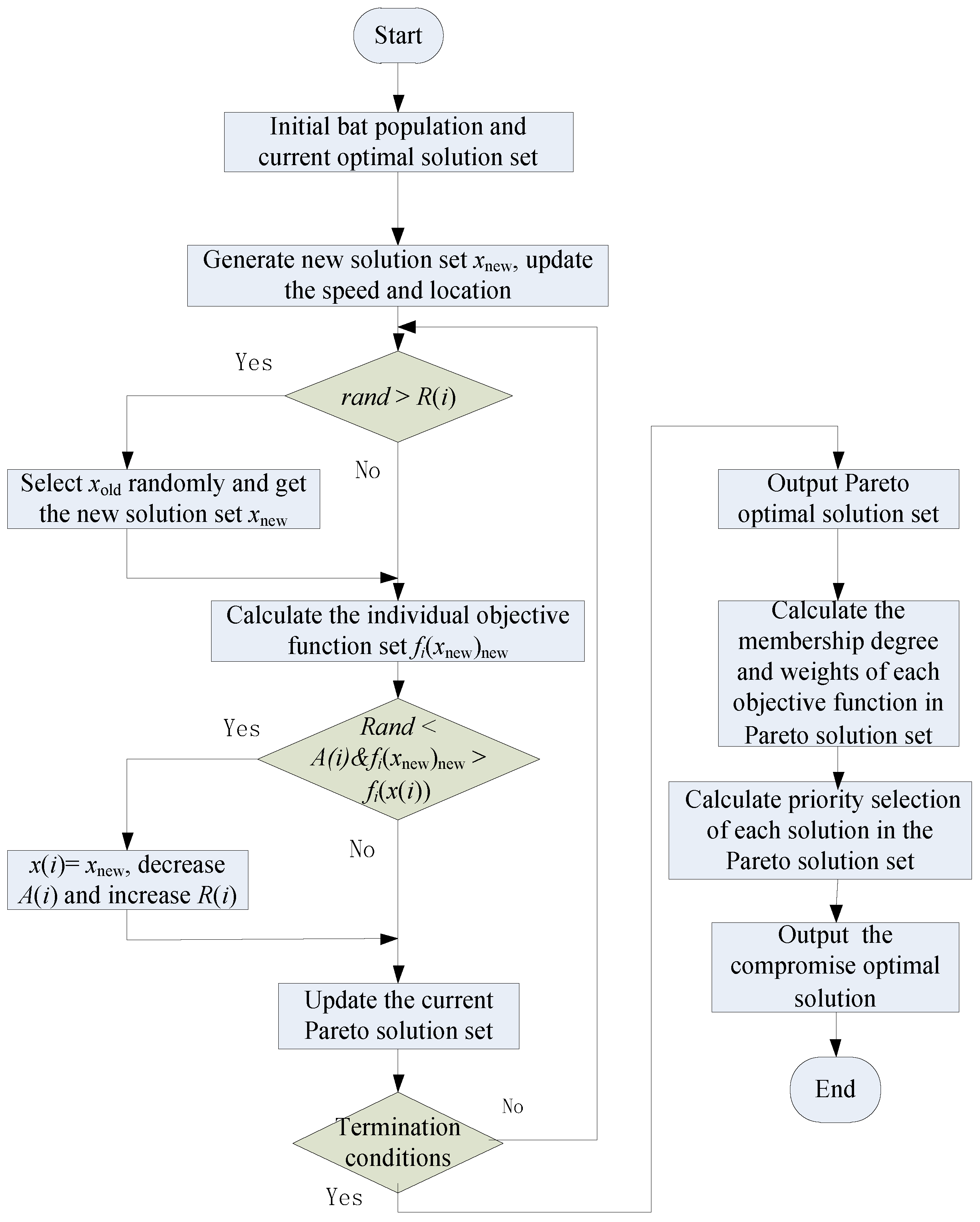
The flow chart of the improved bat algorithm based on the priority selection degree is shown in Figure 5.

5. Example Analysis

5.1. Division of Decision Areas and Determination of Regional Resources

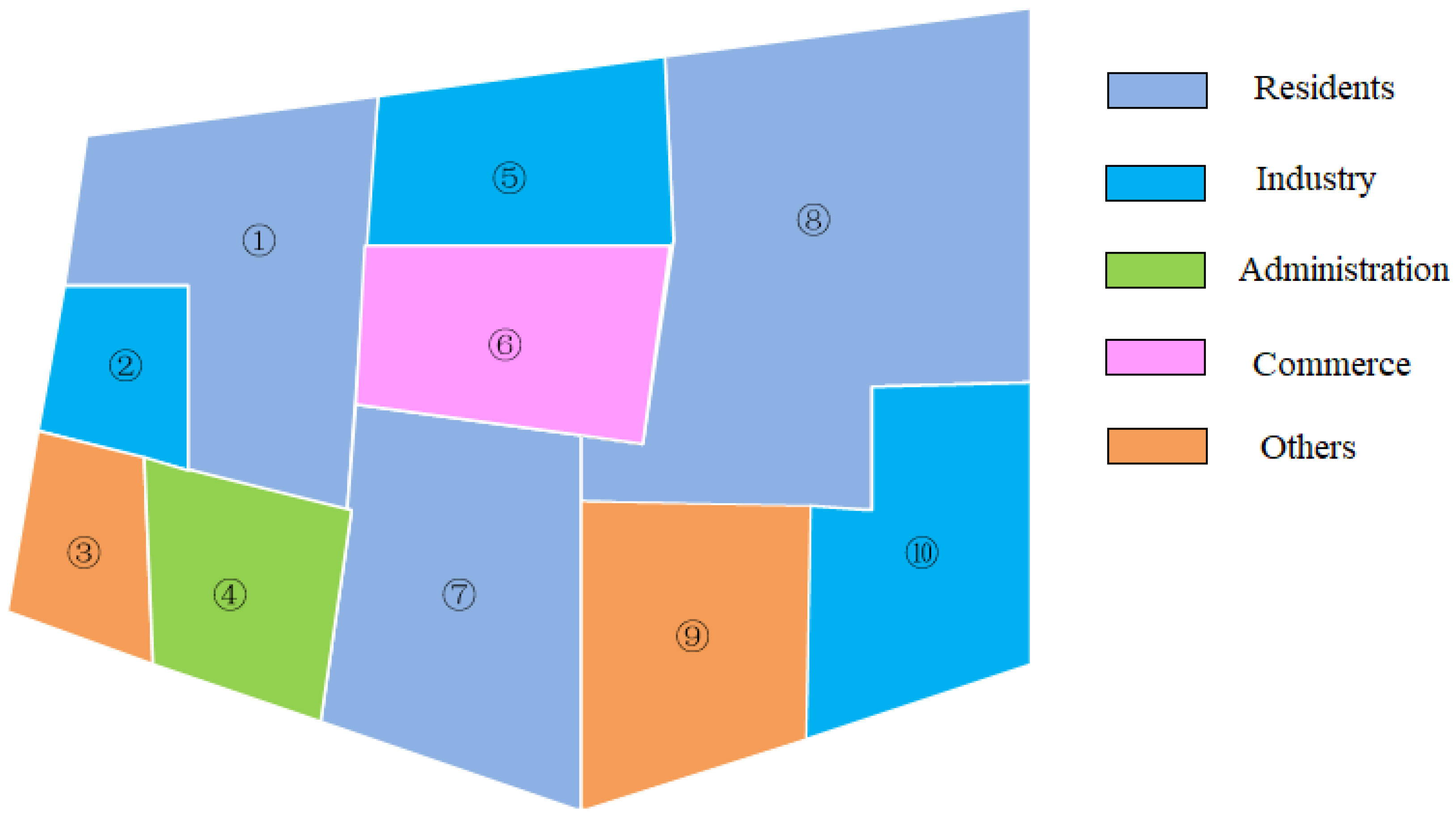
This paper selects a city area and makes a reasonable selection of DG, ES and DR to construct a VPP. Firstly, according to the different regional functions, the decision area of VPP is divided into five categories: residents, industry, administration, commerce and others, as shown in Figure 6.

Obviously, some areas divided according to regional functions have the problem of excessive area acreage and excessive regional resources. If the VPP is built according to the preliminary decision area method, it will be difficult to satisfy the relevant characteristics.

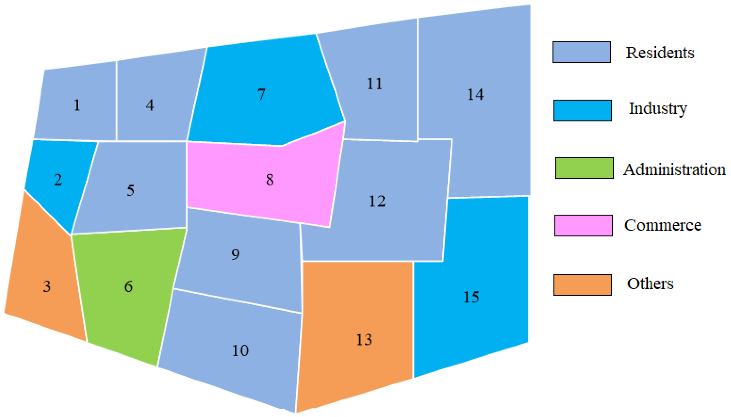
Therefore, the residents, industry, administration, commerce and other areas should be carefully divided according to certain constraints. Under the restriction of area acreage and mixed resources power, the number of areas should be minimized. According to the flow chart in Figure 2, the area eventually can be divided into 15 parts. The numbers and types of all the areas are shown in Figure 7.

The resource type of each area i (i = 1, 2, …, 15) is different. The corresponding decision variables $X_i^{DG}$, $X_I^{ES}$ and $X_I^{DR}$ represent the presence or absence of DG, ES and DR in this area, respectively. 1 represents yes, 0 represents no, and the specific information of each area resource is shown in

Table 1. Distribution of resources in each area.

Resources	1	2	3	4	5	6	7	8	9	10	11	12	13	14	15
DG	1	1	1	1	1	0	1	1	1	0	1	1	1	1	1
ES	1	0	0	1	1	0	0	0	1	1	1	1	0	0	1
DR	1	0	0	1	1	0	0	0	1	1	1	0	0	1	0

.

In Table 1, except for the DG in the 3rd and 13th areas representing the WP and the DG in the rest of the areas is PV. The distribution of resources fully reflects the characteristics of different functional areas. For example, most residential areas have PV generation, DR and ES; commercial areas and administrative areas have less DG, and the installation of wind turbine equipment is more located in a special area, rarely in residential areas, commercial areas and industrial areas.

DG is dominated by WP and PV, and there is a certain degree of complementarity between them. DR means that the power supply side can respond according to the requirements of the power supply department. Moreover, in the peak hours of electricity consumption, certain loads can be reduced to achieve the effect of peak load reduction and valley filling. The ES mainly considers the charging of electric vehicle, and its charging characteristic curve can be obtained through the relevant prediction technology.

5.2. Result Analysis of Virtual Power Plant Construction

In this paper, combining with the daily average time-series characteristic curve of different resources in each area, the resource selection in each region are carried out with the improved bat algorithm based on priority selection. The four elements in the objective function set represent the daily average cost, daily load characteristics, DG consumption degree, and regional aggregation degree, respectively. The value of each objective function is expressed in scientific notation as a*10^b, and the pareto optimal solution set containing 11 solutions is finally obtained, as shown in

Table 2. Optimal solution set of VPP.

Serial Number	Objective Function Set	Area Resources Not Involved in the Construction
1	(2.5, 8.7, 3.3, 1.8)	$X_1^{ES},X_1^{DR},X_2^{DG},X_5^{ES},X_5^{DR},X_9^{DR},X_{11}^{ES}$
2	(2.5, 7.3, 3.3, 1.8)	$X_1^{ES},X_4^{DR},X_9^{DR},X_{10}^{DR},X_{10}^{ES},X_{11}^{ES},X_{12}^{DG}$
3	(2.3, 6.4, 3.2, 1.7)	$X_1^{DR},X_2^{DG},X_4^{DG},X_4^{DR},X_5^{DR},X_{14}^{DG},X_{15}^{DG}$
4	(2.3, 6.3, 3.2, 1.8)	$X_1^{DR},X_4^{DG},X_4^{DR},X_5^{DR},X_{11}^{DG},X_{12}^{DG},X_{14}^{DG}$
5	(2.2, 6.8, 3.2, 1.8)	$X_1^{DG},X_1^{ES},X_4^{DG},X_9^{DG},X_{12}^{DG},X_{12}^{ES},X_{15}^{ES}$
6	(2.2, 5.8, 3.1, 1.7)	$X_1^{DR},X_2^{DG},X_2^{DR},X_{11}^{DG},X_{12}^{DG},X_{14}^{DG},X_{15}^{DG}$
7	(2, 4.1, 2.2, 1.5)	$X_1^{ES},X_1^{DR},X_5^{ES},X_5^{DR},X_{10}^{DR},X_{12}^{DG},X_{13}^{DG}$
8	(1.9, 3.4, 2, 1.1)	$X_2^{DG},X_2^{DR},X_3^{DG},X_9^{ES},X_{11}^{DR},X_{12}^{DG},X_{14}^{DG}$
9	(1.9, 3.5, 2.1, 1.1)	$X_1^{DG},X_1^{ES},X_3^{DG},X_4^{DR},X_8^{DG},X_{11}^{ES},X_{12}^{DG}$
10	(2.1, 4.2, 2.2, 1.1)	$X_1^{DR},X_2^{DG},X_3^{DG},X_4^{DR},X_9^{ES},X_{14}^{DR}$
11	(2.3, 6.7, 3.2, 1.9)	$X_1^{DG},X_1^{ES},X_4^{DG},X_{12}^{DG},X_{12}^{ES},X_{15}^{ES}$

. (The objective function set omits 10^b, and the pareto optimal solution set only lists the area resources which are not involved in the construction).

By calculating the membership degree of the objective function of the 11 solutions, the weight of each objective function is calculated, and the priority selection of each solution is finally obtained. Through the calculation, the variance weights of the four objective functions are 0.21, 0.18, 0.32, and 0.29, respectively. The priority selection of each scheme is obtained by adding the membership degree of each objective function through the weight, as shown in Figure 8.

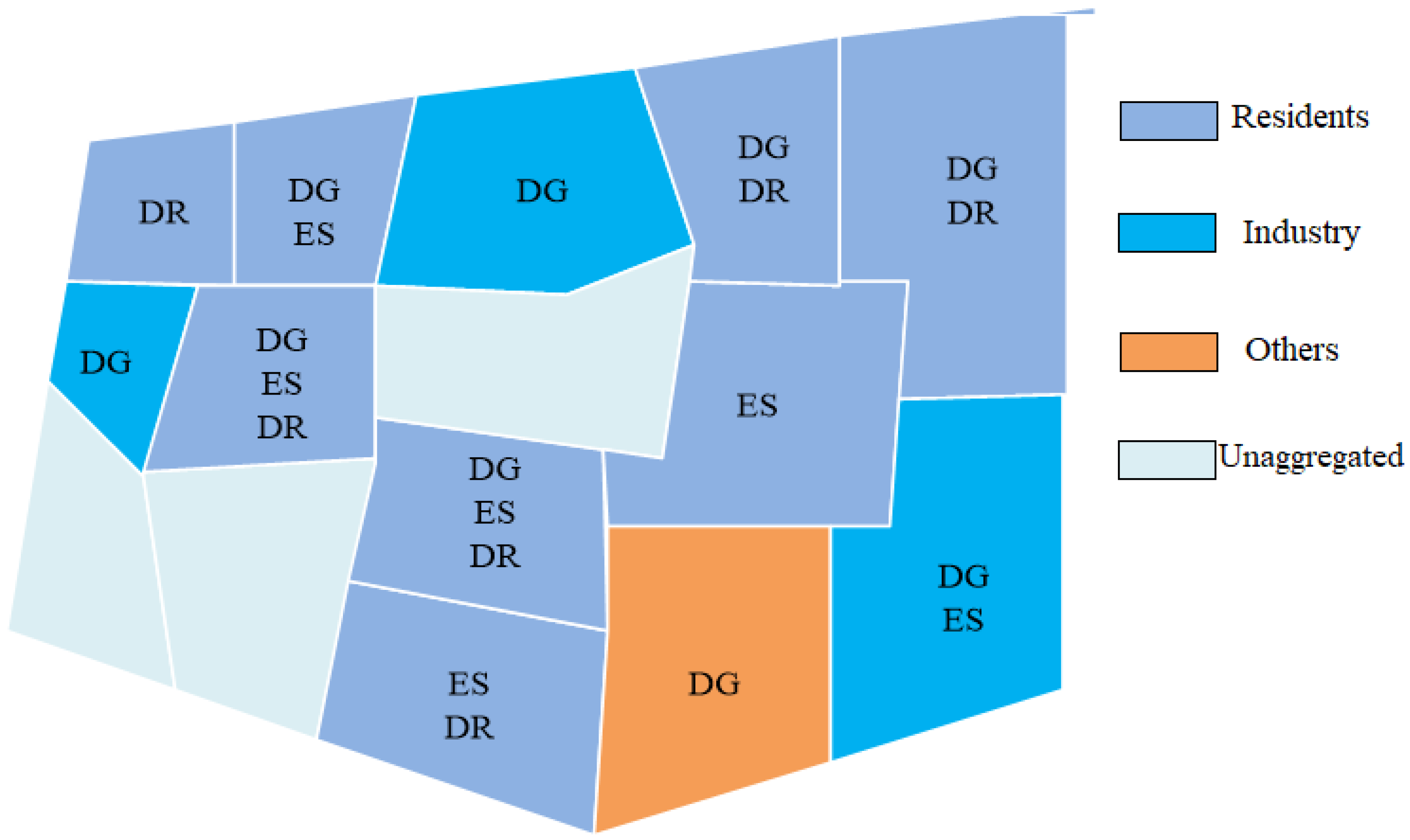
The 9th scheme solution has the highest priority selection, which is 0.71, so it can be chosen as the best compromise optimal solution. The corresponding average daily cost is 19,044 ¥, the volatility is 3.52%, the DG utilization power is 20,505 kW, and the fusion space distance representing the degree of regional polymerization is 1,133,120. The final construction scheme of VPP represented by this solution is shown in

Table 3. Final construction scheme.

Number	1	2	3	4	5	6	7	8	9	10	11	12	13	14	15
DG		✓		✓	✓		✓		✓		✓		✓	✓	✓
ES				✓	✓				✓	✓		✓			✓
DR	✓				✓				✓	✓	✓			✓

(✓ represents the area resources involved in the construction).

It can be seen that the construction of VPP includes various resources, such as PV, WP, ES and DR. Among them, the WP, PV, ES and DR have been used in one area, eight areas, six areas and six areas, respectively. The actual distribution of DER which participates in the aggregation is shown in Figure 9.

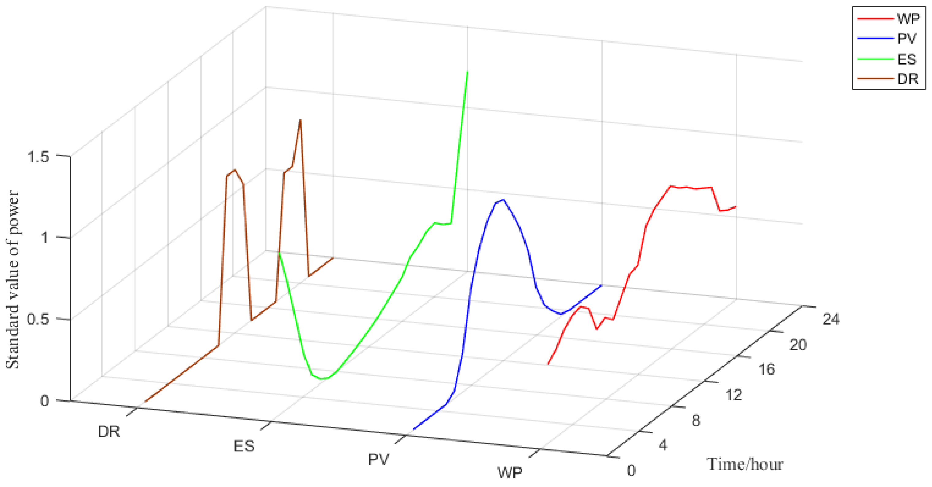
Among the construction of VPP, there are four categories of resources: WP, PV, ES and DR. In order to make the results more intuitive, the power of various loads is standardized. Moreover, the daily characteristic curve of various resources in the entire construction area is shown in Figure 10.

From Figure 10, it can be seen intuitively that there is a clear complementarity in the time series between various resources. The complementary types between any two resources is ${\mathrm{C}}_2^4$ = 6, and the complementary coefficients of various resources are shown in

Table 4. Complementary coefficients of various resources.

Resource Type	Complementary Coefficient
WP, PV	0.2375
WP, ES	0.3100
WP, DR	0.3341
PV, ES	0.3116
PV, DR	0.2534
ES, DR	0.3167

.

The 9th scheme solution is based on the detailed division of decision areas. In order to verify the validity of this method, this scheme is compared with the VPP construction scheme based on the preliminary division of decision areas (the number of each area is shown in Figure 6). The comparison example changes the division of decision area, but the multi-objective optimization model and the solution algorithm remain unchanged. The compromise optimal solution of the comparison example is shown in

Table 5. Construction scheme of the comparison example.

Number	①	②	③	④	⑤	⑥	⑦	⑧	⑨	⑩
DG	✓	✓			✓	✓		✓	✓	✓
ES	✓						✓	✓
DR	✓						✓

(✓ represents the area resources involved in the construction).

The comparison of the two different multi-objective construction models of VPP, which correspond to different decision area division methods, is shown in

Table 6. Comparison of objective function sets.

Number	F1	F2	F3	F4
Detailed division	19,044	3.52%	20,505	1,133,120
Preliminary division	19,121	5.89%	20,406	1,487,020

.

It can be seen from Table 5 and Table 6, F1, F2, F3 and F4 represent the daily average cost, daily load characteristics, DG consumption degree, and regional aggregation degree, respectively. The smaller the values of F1, F2 and F4 are, the better the model construction effect is, while F3 is the opposite. As shown in Table 6, the VPP construction scheme corresponding to detailed division method is better than the other one, especially in terms of the daily load characteristics and regional aggregation degree.

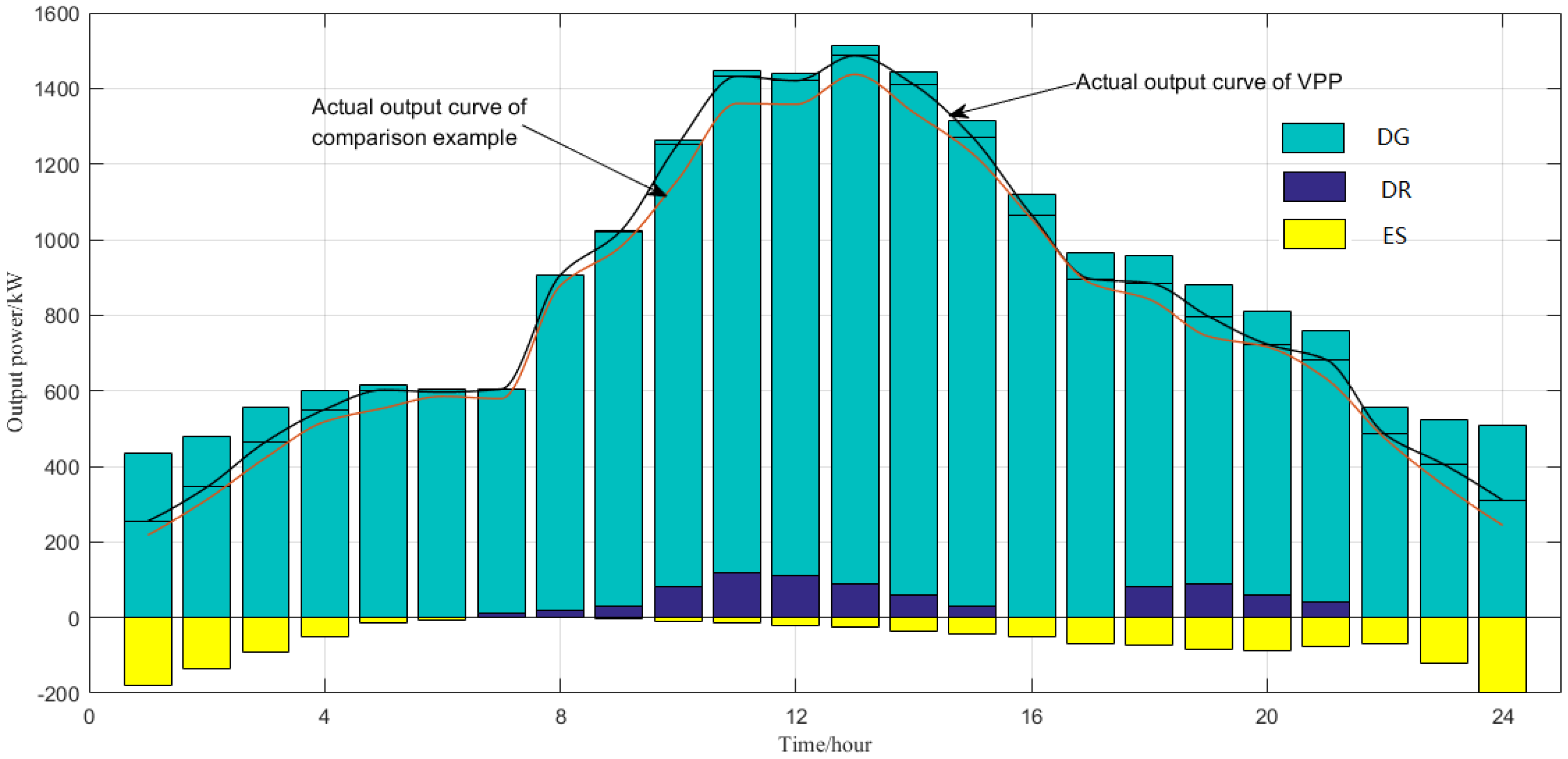
The construction of VPP according to the 9th scheme takes into account the cost, load characteristic, DG consumption and degree of resource aggregation. The actual output curve of the VPP is superimposed by the WP, PV, ES and DR. In addition, the output curve of the proposed scheme is superior to the output curve of the comparison example in terms of output size and curve volatility, as shown in Figure 11 (including the output curve of the comparison example).

The planed output curve of VPP is determined by the daily characteristic curve of DER. It can be seen from Figure 11, DG accounts for the overwhelming majority of the output of VPP, and a part of DR is also involved in the output of VPP. The ES in this paper serves as an electric device, similar to an electric vehicle; therefore, the columnar graph of the ES is shown in the lower part of the coordinate axis. Finally, these three kinds of resources are superimposed to obtain the actual output curve of VPP.

6. Conclusions

In the construction of a VPP, the method of making decisions on each resource in the whole area will bring about a disaster of dimensionality in calculation. This paper firstly divides the decision area of the VPP, reduces the decision variables at the time of aggregation and then determines the decision variables of the model. Then, a multi-objective optimization model, which takes into account the average daily cost, load characteristics, degree of DG consumption and degree of resource aggregation, is established. Finally, the improved bat algorithm based on priority selection is used to solve the model to obtain an optimal compromise solution. Through the example analysis, we can get:

(1)

The decision variables are used to represent all kinds of DER in each area; therefore, the final construction results of VPP are more intuitive.

(2)

The compromise selection of the multiple optimal solutions is achieved through the priority selection, and a compromise optimal solution can be obtained which provides an effective reference for planners.

(3)

The actual VPP output curve obtained by this example is generally determined by the output curve of DG, ES and DR, which play an auxiliary regulatory role.

In addition, the further work is needed to consider the uncertainty of some DER output. Some uncommon DER models, such as pumped storage and hydroelectric, can be studied, and the environmental problems also need to be considered in the model construction. Moreover, the decision area can be linked to a real physical topology of the distribution network part. Finally, the study of a single VPP can be extended to multiple VPPs and the relationship between multiple VPPs also can be considered.

References

- Petersen, M.K.; Hansen, L.H.; Bendtsen, J.; Edlund, K.; Stoustrup, J. Market Integration of Virtual Power Plants; IEEE: New York, NY, USA, 2013; pp. 2319–2325. [Google Scholar]
- Dabbagh, S.R.; Sheikh-El-Eslami, M.K. Risk-based profit allocation to DERs integrated with a virtual power plant using cooperative Game theory. Electr. Power Syst. Res. 2015, 121, 368–378. [Google Scholar] [CrossRef]
- Ehsan, A.; Yang, Q. Optimal integration and planning of renewable distributed generation in the power distribution networks: A review of analytical techniques. Appl. Energy 2018, 210, 44–59. [Google Scholar] [CrossRef]
- Fang, X.; Yang, Q.; Wang, J.; Yan, W. Coordinated dispatch in multiple cooperative autonomous island microgrids. Appl. Energy 2017, 162, 40–48. [Google Scholar] [CrossRef]
- Sun, Y.; Li, H.; Yang, W.; Gao, Y. Optimized Aggregation Model for Resident Users Based on SOM Demand Response Potential. Electr. Power Constr. 2017, 38, 25–33. [Google Scholar]
- Mnatsakanyan, A.; Kennedy, S.W. A Novel Demand Response Model with an Application for a Virtual Power Plant. IEEE Trans. Smart Grid 2014, 6, 230–237. [Google Scholar] [CrossRef]
- Cao, C.; Xie, J.; Yue, D.; Huang, C.; Wang, J.; Xu, S.; Chen, X. Distributed Economic Dispatch of Virtual Power Plant under a Non-Ideal Communication Network. Energies 2017, 10, 235. [Google Scholar] [CrossRef]
- Nosratabadi, S.M.; Hooshmand, R.A.; Gholipour, E. Stochastic profit-based scheduling of industrial virtual power plant using the best demand response strategy. Appl. Energy 2016, 164, 590–606. [Google Scholar] [CrossRef]
- Helms, T.; Loock, M.; Bohnsack, R. Timing-based business models for flexibility creation in the electric power sector. Energy Policy 2016, 92, 348–358. [Google Scholar] [CrossRef]
- Dong, W.; Wang, Q.; Yang, L. A coordinated dispatching model for a distribution utility and virtual power plants with wind/photovoltaic/hydro generators. Autom. Electr. Power Syst. 2015, 39, 75–81. [Google Scholar]
- Wang, J.; Yang, W.; Cheng, H.; Huang, L.; Gao, Y. The Optimal Configuration Scheme of the Virtual Power Plant Considering Benefits and Risks of Investors. Energies 2017, 10, 968. [Google Scholar] [CrossRef]
- Ju, L.; Tan, Z.; Yuan, J.; Tan, Q.; Li, H.; Dong, F. A bi-level stochastic scheduling optimization model for a virtual power plant connected to a wind–photovoltaic–energy storage system considering the uncertainty and demand response. Appl. Energy 2016, 171, 184–199. [Google Scholar] [CrossRef] [Green Version]
- Tan, Z.; Wang, G.; Ju, L.; Tan, Q.; Yang, W. Application of CVaR risk aversion approach in the dynamical scheduling optimization model for virtual power plant connected with wind-photovoltaic-energy storage system with uncertainties and demand response. Energy 2017, 124, 198–213. [Google Scholar] [CrossRef]
- Ju, L.; Li, H.; Zhao, J.; Chen, K.; Tan, Q.; Tan, Z. Multi-objective stochastic scheduling optimization model for connecting a virtual power plant to wind-photovoltaic-electric vehicles considering uncertainties and demand response. Energy Convers. Manag. 2016, 128, 160–177. [Google Scholar] [CrossRef]
- Kasaei, M.J.; Gandomkar, M.; Nikoukar, J. Optimal Operational Scheduling of Renewable Energy Sources Using Teaching-Learning Based Optimization Algorithm by Virtual Power Plant. J. Energy Resour. Technol. 2017, 139, 062003. [Google Scholar] [CrossRef]
- Xia, Y.H.; Liu, J.Y.; Huang, Z.W.; Zhang, X. Carbon emission impact on the operation of virtual power plant with combined heat and power system. Front. Inf. Technol. Electron. Eng. 2016, 17, 479–488. [Google Scholar] [CrossRef]
- Pandžić, H.; Kuzle, I.; Capuder, T. Virtual power plant mid-term dispatch optimization. Appl. Energy 2013, 101, 134–141. [Google Scholar] [CrossRef]
- Giuntoli, M.; Poli, D. Optimized Thermal and Electrical Scheduling of a Large Scale Virtual Power Plant in the Presence of Energy Storages. IEEE Trans. Smart Grid 2013, 4, 942–955. [Google Scholar] [CrossRef]
- Kardakos, E.G.; Simoglou, C.K.; Bakirtzis, A.G. Optimal Offering Strategy of a Virtual Power Plant: A Stochastic Bi-Level Approach. IEEE Trans. Smart Grid 2016, 7, 794–806. [Google Scholar] [CrossRef]
- Faqiry, M.N.; Edmonds, L.; Zhang, H.; Khodaei, A.; Wu, H. Transactive-Market-Based Operation of Distributed Electrical Energy Storage with Grid Constraints. Energies 2017, 10, 1891. [Google Scholar] [CrossRef]
- Wei, L.; Zhao, B.; Wu, H.; Zhang, X. Optimal Allocation Model of Energy Storage System in Virtual Power Plant Environment with a High Penetration of Distributed Photovoltaic Generation. Autom. Electr. Power Syst. 2015, 23, 66–74. [Google Scholar]
- Sun, S.; Yang, Q.; Yan, W. A novel Markov-based temporal-SoC analysis for characterizing PEV charging demand. IEEE Trans. Ind. Inform. 2018, 14, 156–166. [Google Scholar] [CrossRef]
- Ai, X.Y.; Gu, J.; Xie, D. Forecasting Method for Electric Vehicle Daily Charging Curve. Proc. CSU-EPSA 2013, 25, 25–30. [Google Scholar]
- Schwarz, H.; Cai, X.S. Integration of renewable energies, flexible loads and storages into the German power grid: Actual situation in German change of power system. Front. Energy 2017, 11, 107–118. [Google Scholar] [CrossRef]
- Sun, L.L.; Gao, C.W.; Tan, J.; Cui, L.; College, C. Load Aggregation Technology and Its Applications. Autom. Electr. Power Syst. 2017, 41, 159–167. [Google Scholar]
- Jiang, Y.Q.; Wong, S.C.; Zhang, P.; Choi, K. Dynamic Continuum Model with Elastic Demand for a Polycentric Urban City. Transp. Sci. 2017, 51, 931–945. [Google Scholar] [CrossRef]
- Gong, W.; Liu, J.; He, X.; Liu, Y. Load Restoration Considering Load Fluctuation Rate and Load Complementary Coefficient. Power Syst. Technol. 2014, 38, 2490–2496. [Google Scholar]
- Yang, X.S. A New Metaheuristic Bat-Inspired Algorithm. Comput. Knowl. Technol. 2010, 284, 65–74. [Google Scholar] [Green Version]
- Yang, Y.; Wang, X.; Luo, J.; Duan, J.; Gao, Y.; Li, H.; Xiao, X. Multi-Objective Coordinated Planning of Distributed Generation and AC/DC Hybrid Distribution Networks Based on a Multi-Scenario Technique Considering Timing Characteristics. Energies 2017, 10, 2137. [Google Scholar] [CrossRef]
Figure 1.
The illustration of the constitution of virtual power plant.
Figure 2.
Flow chart of decision area division of VPP.
Figure 3.
Preliminary division of decision area of VPP.
Figure 4.
Detailed division of decision area of VPP.
Figure 5.
Flow chart of the improved bat algorithm based on priority selection.
Figure 6.
The result of preliminary division of decision area.
Figure 7.
The result of detailed division of decision area.
Figure 8.
The priority selection of each scheme.
Figure 9.
Distribution of distributed energy resources.
Figure 10.
Daily characteristics curve of various resources.
Figure 11.
Output curve of VPP.