Inverse Analysis of Cellulose by Using the Energy-Based Method and a Rotational Rheometer


Chair of Continuum Mechanics and Constitutive Theory, Institute of Mechanics, Technische Universität Berlin, Einsteinufer 5, 10587 Berlin, Germany
Appl. Sci. 2018, 8(8), 1354; https://doi.org/10.3390/app8081354
Submission received: 25 July 2018
/
Revised: 7 August 2018
/
Accepted: 10 August 2018
/
Published: 12 August 2018
(This article belongs to the Section Materials Science and Engineering)
Abstract
:Featured Application
It is beneficial to have a clear method for determining material parameters, especially in the case of nonlinear material models. For soft materials, several material models exist, and an engineer can try out these different material models by using the method presented herein.
Abstract
Biological and polymer-type materials usually show a complicated deformation behavior. This behavior can be modeled by using a nonlinear material equation; however, the determination of coefficients in such a material equation is challenging. We exploit representation theorems in continuum mechanics and construct nonlinear material equations for cellulose in an oscillatory rheometer experiment. The material parameters are obtained by using the energy-based method that generates a linear regression fit even in the case of a highly nonlinear material equation. This method allows us to test different nonlinear material equations and choose the simplest material model capable of representing the nonlinear response over a broad range of frequencies and amplitudes. We present the strategy, determine the parameters for cellulose, discuss the complicated stress-strain response and make the algorithm publicly available to encourage its further use.
1. Introduction
Especially in polymer science and biological tissue modeling, the material response fails to be modeled accurately by a linear material equation. For a fluid-like material, Newtonian material model establishes a linear connection between stress and velocity gradient. The material coefficient, called viscosity, is a constant, and since a constant fails to attain an accurate modeling, there are various approaches to increase the complexity by choosing a viscosity depending on the velocity gradient [1]. There are several proposals about developing such nonlinear material (constitutive) equations starting from a microstructure or using chain interactions, as well as exploiting thermodynamical reasoning. There are various nonlinear models in the literature. None of them are delivering accurate results for all applications. For example, widely-used models as in [2,3,4] have been modified by [5,6] in order to obtain models providing results for different scenarios. Even the modified version was criticized in [7], and a possible modification was proposed in [8]. In order to include a rate, the objective time derivative was proposed by [9]. Instead of a material equation with a rate, integral equations were proposed in order to include the full history on deformation as in [10,11]. These equations were used as models in [12], and measurements were undertaken in [13]. However, in numerical mechanics, integral equations are more challenging to implement than differential equations. Hence, in this paper, we (author and reader) will benefit from representation theorems to generate nonlinear material equations; as already used in [14,15,16,17]. As stated in [18], the nonlinear modeling in rheology is still an open question, and we cannot expect to acquire a consensus; but we need tools making the inverse analysis for different suggestions possible. Such tools may lead to easier comparisons of different models. In this work, we present and use an approach capable of delivering coefficients for nonlinear material equations.
Cyclic measurements by using a rotary viscometer (rheometer) are optimized for linear rheology, where the material coefficients are constants. The output of such a measurement is given as two moduli, one modulus for elastic behavior and another modulus for viscous behavior. This interpretation is valid and appropriate for a linear material model. In the case of a nonlinear material behavior, we fail to investigate the elastic and viscous effects separately in these moduli. Thus, we need to extract the data in such a way that the coefficients in a nonlinear material model can be determined. A considerable amount of literature has been published in the last two decades. Among others, for example as in [19,20,21,22,23,24,25], various polynomial expansion techniques have been proposed in order to fit the experimental data. As shown in [26], they have mathematical similarities. In order to apply them, a revision is necessary of the control unit of a conventional rheometer. Newer devices deliver such functionality, so their approach is possible, but in a way also limited to the existing measurement device.
An energy-based method was proposed in [27] (Section 9) and applied in [28]. By using the energy-based method, we generate a linear regression problem out of the conventional output of an oscillatory measurement in a rheometer even in the case of nonlinear material equations. In a linear regression problem, the solution is unique and computationally far easier than any nonlinear regression problem. Hence, by using the energy-based method, an experimentalist can quickly try different material equations by increasing the complexity step by step. We emphasize that the inverse analysis lasts less than a minute on a moderate computer. The optimization is fast simply because of the linear regression. Hence, the whole method can be described as the approach for how to create a linear regression problem in the case of a nonlinear material equation.
The underlying work consists of three main sections. First, we explain the standard measurements of a polymeric carbohydrate, namely cellulose. We use the results of oscillatory measurements performed on a rotary viscometer. Such measurements are challenging in the case of a nonlinear response; see [29,30]. The probe was sheared by giving a harmonic stress function as the input. The outputs of these measurements were the elastic or storage modulus, , and the viscous or loss modulus, , as functions of the frequency and amplitude of the input function. Secondly, we present very briefly the tensor representation theorems and show a strategy to generate different material models. Other models can be used, as well, and we only present one possible method for how to construct more complicated material models to describe the physics. In this paper, the main goal is to present the energy-based method in action. Therefore, thirdly, a concrete example is presented. We analyze the material by applying the method and find out the simplest material equation modeling the measured nonlinear behavior. We discuss its stress-strain behavior in order to demonstrate the nonlinear character of the applied material model.
2. Materials and Method of Measurement
A nonlinear polymer has been selected for experimental analysis. Cellulose was discovered in 1838 by Anselme Payen, and it became the most common organic polymer [31]. Cellulose is a polymeric carbohydrate with repeating hydroxy groups of -1,4 linked D-glucose units of six-carbon monosaccharides; thus, its chemical formula reads (CHO). These hundreds to thousands of repeating units form linear chains. In order to produce individual cellulose microfibrils from the pulp, 2,2,6,6-tetramethylpiperidine 1-oxyl (known as TEMPO)-mediated oxidation was followed by a mechanical treatment such that the lengths of microfibrils were 1–2 m and the widths of microfibrils were 3–4 nm, corresponding to a parallel bundle of 5–7 cellulose chains. Sonication and ultracentrifugation were subsequently used for removing large aggregates. The progress was observed under an optical microscope, and the Brunauer–Emmett–Teller (BET) surface area was determined as m/g. The original suspension of nanofibrillated cellulose in pure water had a concentration of 0.125 wt %, and by using evaporation, the suspension of 0.74 wt % was prepared and used for the experiments.
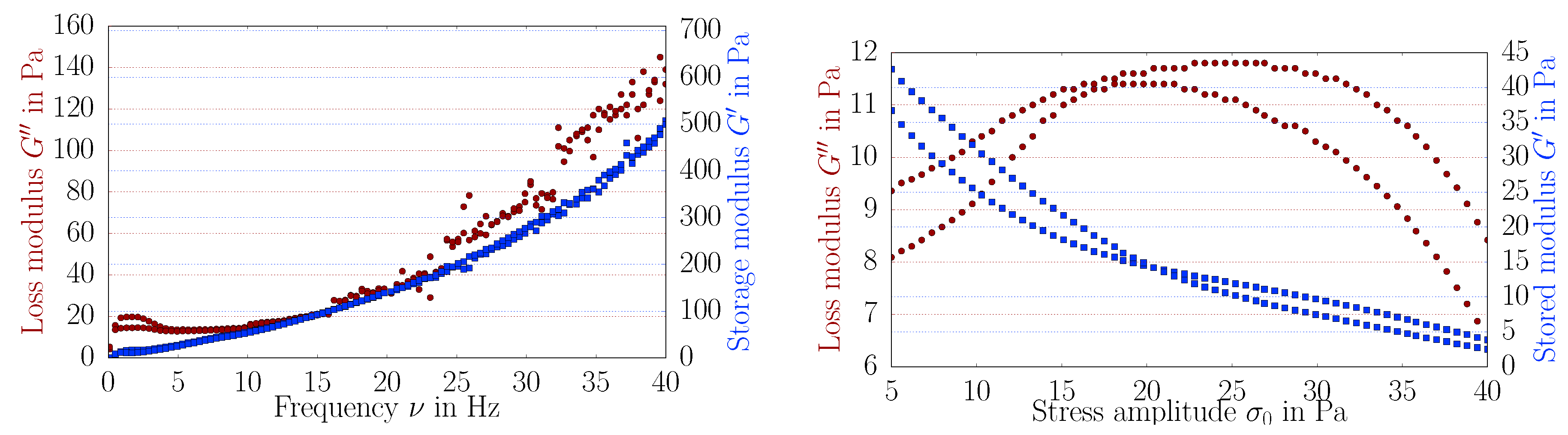
All preparations and measurements were performed by the group of Prof. V. Kocherbitov at the Biomedical Laboratory, Malmö University, and the dataset is published in [32]. A standard rotational viscometer, namely the Bohlin CVO rheometer from Malvern Instruments, with a cone-plate configuration, was selected with a steel cone of 40 mm in diameter and a 4° cone angle, with the truncated apex at 150 m to eliminate any contact between the cone and plate. After calibrating and placing the sample limited to the circumference, the cone and probe were covered with a plastic lid to avoid evaporation. All experiments were performed at 20 °C. With the same sample, a standard amplitude sweep and a frequency sweep were performed by controlling the shear stress; see Figure 1 for the results. A harmonic excitation was achieved by steering the shear stress with a given frequency and amplitude. For the amplitude sweep, the frequency was fixed at 1 Hz, and the amplitude was varied from 5–40 Pa. Analogously, for the frequency sweep, the amplitude was kept constant at 40 Pa, and the frequency was varied from 0.1–40 Hz. Each experiment was repeated two times, and all data are shown in Figure 1 by means of the so-called storage and loss moduli.
The represented experimental data are an example to present the strategy used in this work. Because of the highly-nonlinear character of the material, especially the frequency sweep has noise between 20–25 Hz. Furthermore, the precision of the amplitude sweep is low. However, we emphasize that the methodology explained in the next sections is not susceptible to experimental inaccuracies and performs well even under high repeatability errors.
3. Nonlinear Material Equations and the Energy-Based Method for the Inverse Analysis
In continuum mechanics, a Eulerian frame is used for a viscous fluid, where coordinates, x, denote the spatial positions. By using Cartesian coordinates, the velocity of a fluid particle currently at at the present time t is denoted by . Since the velocity of each fluid particle is challenging to monitor separately, in a rheometer measurement, the measurand of a system is the energy, E. The temperature is held constant such that the process is isothermal. In an isothermal process, the energy can be calculated in a domain of interest, , herein within the sample, for a period of time, , as follows:
where a comma indicates a partial derivative in space, and we understand a summation over every repeated index, known as Einstein’s summation convention. Cauchy’s stress, , is symmetric for non-polar materials such that we can rewrite the energy:
since the antisymmetric part of the velocity gradient vanishes by contracting it to the symmetric stress tensor. The symmetric part of the velocity gradient, , and the symmetric Cauchy stress, , are related by a material (or constitutive) equation. We aim at constructing this material equation and then at determining its coefficients.
In a rheometer, the energy is monitored precisely by measuring the electric power from the wall (minus the standard induction motor’s losses). The rheometer shears the sample, say, on the -plane, and holds the distance of the plates fixed such that . Hence, the velocity gradients read:
We know that for stress, more than the shear stress occurs in many materials. However, the velocity gradient has only shear terms even in the nonlinear case.
Instead of using this energy, in linear rheology, the storage and loss moduli are introduced. We will briefly explain their use and suggest a strategy to extract more information out of them. In the case of a stress-steered rheometer, a harmonic input for the shear component of stress is applied, written in an exponential form (in order to include sinus and co-sinus functions together):
Usually, it is assumed that the material response is collinear such that only a shear component of the symmetric velocity gradient appears. Moreover, in linear rheology, the strain rate is approximated as equal to the velocity gradient, , such that a linear response:
allows us to rewrite:
and propose a relation between stress and strain:
For a linear material, relates to the elastic modulus; relates to the viscosity since:
In order to determine and from the energy, we use:
since the velocity gradient in Equation (3) consists of only shear components. For a detailed analysis by using spherical coordinates, we refer to [27] (Section 8). By using a cone-plate or a small plate-plate geometry, we can justify the assumption of constant stress and strains within the sample such that we obtain the following energy density (energy per volume):
where V is the volume of the sample. Since the measurement is a shear experiment, we assume that the volume remains the same throughout the experiment. We use a sinusoidal excitation, , meaning that we need to employ the imaginary part,
As we have the relation, , we acquire:
such that:
For notational simplicity, we introduce:
Now, we can calculate the energy density under the aforementioned sinusoidal stress input,
Consider first the energy measured over the entire period, ,
which denotes the dissipated energy after one cycle. In a so-called Lissajous–Bowditch curve (stress on the abscissa and strain on the ordinate), the area inside the hysteresis loop is the dissipated energy. Secondly, consider the energy measured over the quarter period, ,
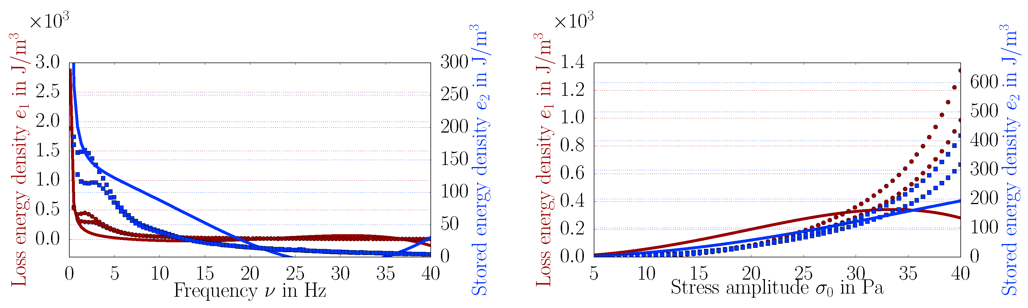
which indicates the stored energy within the quarter period. Instead of using and , we will use and as the output of the experiment. For a measurement at a specific (angular) frequency, , and amplitude, , we have , values. By varying the frequency and amplitude, we acquire a set of energies as observables. For the aforementioned measurements, the energies are plotted in Figure 2.
For the sake of clarity, we sum up. Output from a conventional rheometer is given as and for an amplitude and frequency range. This output can easily be transformed into and , for any set of measurements. This form is more useful than and since the real measurand is the energy. In order to present the idea clearly, the new outcome of energies and have the following relations:
for any non-polar material, with a linear or a nonlinear response. Since we use a stress-steered measurement, we aim at finding a relation of depending on .
3.1. Constructing Nonlinear Material Equations
For generating material equations, we use tensor representation theorems. For a more detailed introduction, we refer to [28] (Section 4). Since stress is the controlled parameter, we search for a functional relation, where depends on , in other words, we aim for . For an isotropic material, the most general form of such an equation reads:
The material coefficients, , , , are scalar functions depending on the stress via its invariants,
The first invariant, , is linear in ; the second invariant, , is quadratic in ; the third invariant, , is cubic in . The relation in Equation (19) represents the general equation in three-dimensional space. We can construct material equations in any complexity. In order to present it, we generate first a linear equation:
where , , are material constants to be determined by an inverse analysis. If and vanish for a material, the result is often called a Newtonian or Stokes fluid. Analogously, we can generate a quadratic equation:
or even a cubic equation:
The nonlinearity can be increased by using a polynomial decomposition. Instead of a polynomial function, we can apply a trigonometric function, capturing the nonlinearities successfully. We propose to use a sigmoid model:
The idea of using such a model is based on [33]; some applications and analysis about the behavior of such a material equation can be found in [34,35,36]. The sigmoid model allows a sharp change between positive and negative values of with a differentiable function . Hence, it is an adequate model for computations, as well as it captures high nonlinearities in materials’ response, as well.
In this straight-forward way, we can easily construct more complicated material equations by adding a rate-dependency. We will see that the following material model:
will be modeling the nonlinear response of the underlying material in experiments. The stress rate has to be an objective rate as in [9]. We will approximate it by a partial derivative for the sake of simplicity.
3.2. Inverse Analysis
The observables from a measurement are and for a set of frequencies and amplitudes. Suppose we want to try to fit the experimental data by using the sigmoid model as posed in Equation (24). Stress is the controlled variable:
and even normal stresses occur; we assume that the stress is deviatoric such that its trace (sum of diagonal components) vanishes. The sigmoid model has the following shear response:
With the help of Equation (18), we can now calculate the energies, and . We start with:
with:
since are constants. Analogously, we can calculate:
with:
We can rearrange in the form of a matrix A. Every component of A can be calculated for a measurement with the known function. The matrix A is for a specific frequency, , and amplitude, . Unknowns are the two material constants, . We already have discussed the measurement data in Equations (16) and (17), so we may rewrite a measurement for a specific frequency, , and amplitude, , as follows:
Suppose we have m measurements with different frequencies, viz., , , , ⋯, , at a specific amplitude. Moreover, we have n measurements with different amplitudes, , , , ⋯, , at a specific frequency. Then, the matrix A will be as follows:
By using linear algebra, we write all measurements:
where the unknowns, , are collected as above and the experimental results, b, for each frequency and amplitude are written among each other. This reformulation indicates that the problem is linear in ; in other words, it is an optimization problem of linear regression. The unknowns can be calculated uniquely by using the normal equation in statistics:
we refer to [28] (Section 6.1.1) for its well-known derivation based on the least squares minimization. It is important to recap that we have arrived at a linear regression problem with a unique set of solutions. In other words, the material constants obtained in this way are the only parameters matching the experiments by means of a least squares fit. Although the material equation is highly nonlinear, we exploited the energy-based method and found a way of determining the parameters just by solving a simple matrix multiplication.
4. Results
We have presented the measurements and the energy-based method for determining the material constants of a nonlinear material equation. From the measurements, we construct the b vector. The matrix of integrals, A, is generated by computing the integrals numerically with Simpson’s rule. We use standard numerical techniques accessible via open-source packages in Python language. Concretely, we employ NumPy [37] for computation and MatPlotLIB [38] for visualization. It is of paramount importance to recall that the solution of the material constants are unique since we solve a linear regression problem. The computation is only some linear algebra steps lasting no more than a minute (Python running in an Ubuntu 14.04 working on a single Intel Core i7-4650U with a 1700-MHz processor).
We start with a linear model and increase the complexity as explained in the latter section. Every trial is accomplished quickly owing to the energy-based method. In order to present the followed strategy clearly, we start with the linear material equation,
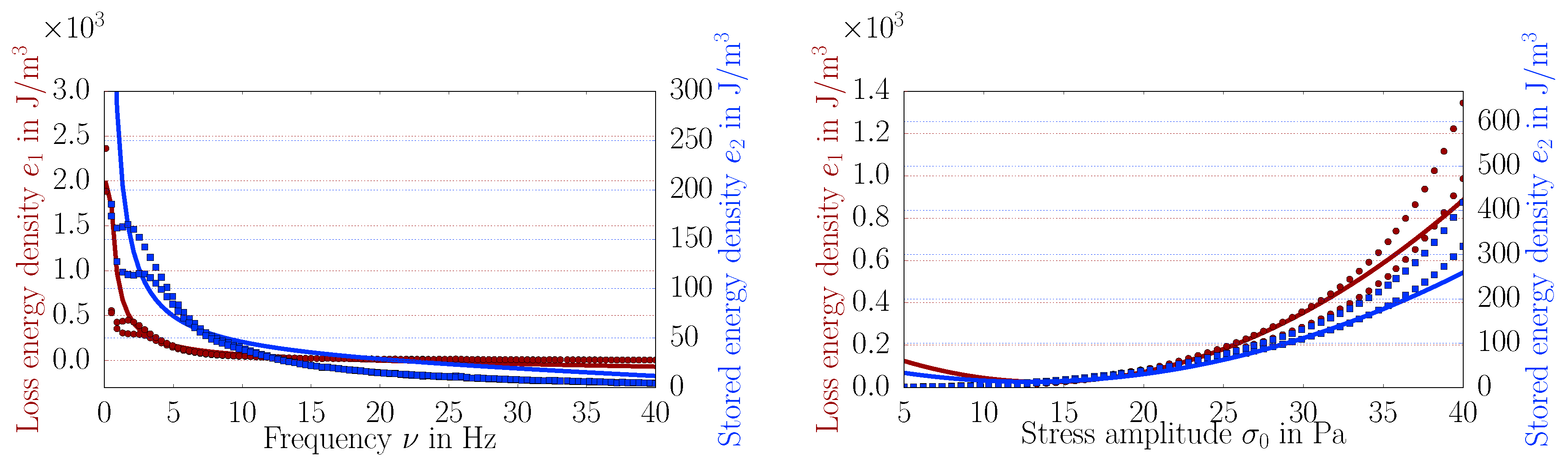
where the rate of stress is involved such that we may name it the Maxwell model. We apply the code for determining , , and plot experiments as dots and the material model as continuous lines in Figure 3.
The lower frequencies and small amplitudes can be approximated with this model. For higher frequencies and amplitudes, this model fails to approximate the behavior. Therefore, we try a more complicated model and determine the material parameters for the following cubic model:
This time, 12 material constants are obtained by using the code. Although the material equation is highly nonlinear, by using the energy-based method, we determine all of these material constants uniquely. With this cubic model, higher frequencies are modeled better; however, the general accuracy is limited, and actually, amplitudes cannot be modeled at all; see Figure 4.
Finally, we have applied the sigmoid model in different configurations and chosen the simplest model with only six material constants,
This model is capable of capturing the materials responses as accurately as possible. By setting Pa, Pa s, Pa s, we have obtained the following material constants:
The fit with the sigmoid model is shown in Figure 5.
It is obvious that the fit with the sigmoid model is better than linear and cubic models. Especially in the variation of frequency, the sigmoid model performs an accurate fit at the lower, as well as the higher values. The linear model does not capture higher frequencies well. The cubic model is missing the expected accuracy. The sigmoid model performs an adequate fit in the whole interval of amplitude sweep. Linear and cubic models are simply not capable of fitting higher amplitudes; but the sigmoid model shows a good agreement with experimental data.
It is important to address the lack of precision in the data. This fact is caused by extremely high stress amplitudes for this soft matter. Under 40 Pa of stress, depending on the frequency, the material can reach strain values around three (meaning 300% of stretching). Therefore, such measurements are challenging, and the lack of precision is fair. The quality of fit relies on the data’s precision. We fit at once all different measurements and variations. In total, we use eight datasets: two energies from two different measurements for amplitude and frequency variations. Since we use linear regression minimizing the squared error between measurement and estimation, using two different measurements is equal to constructing a geometric mean of these measurements and then fit. We emphasize that for all datasets, the same material equation with the same material parameters is used to capture all of these effects.
The sigmoid model performs with very good results only by using six parameters. The fit is in agreement for a large range of amplitudes and frequencies. As previously mentioned, for this kind of soft matter, the stress amplitude is large, providing a remarkable viscous character of the material, as well. In order to study this response, we exploit Lissajous–Bowditch plots. By applying the following harmonic shear stress:
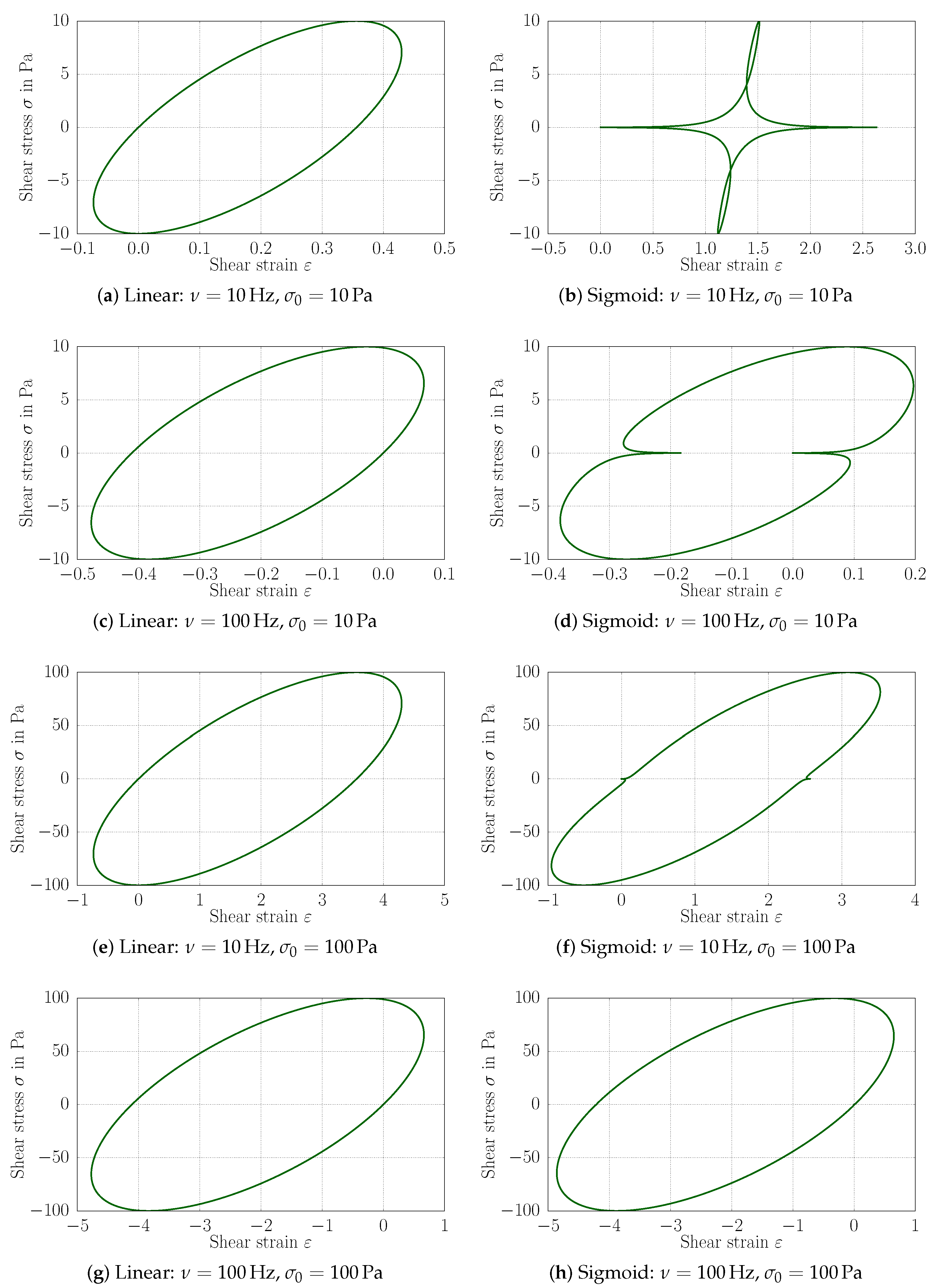
we solve numerically the strain by using the linear model as in Equation (36), as well as the sigmoid model as in Equation (38). By using the fit parameters as in Equation (39), we obtain the response as shown in Figure 6.
The linear model presents the same response function in lower, as well as higher frequencies and amplitudes. Conceivably, the sigmoid model presents different responses for the different amplitudes and frequencies. In the case of the high frequency and amplitude (see Figure 6h), the response is identical to the linear model. The value of the high frequency and amplitude depends on the material parameters; for the material used, 100 Hz and 100 Pa seem to be high enough. For lower frequencies and amplitudes, the response of the linear model remains the same; however, the sigmoid model shows a complex response. Indeed, we know that non-circular curves were reported previously by measuring the stress over shear; see for example [21] (Figure 9), [39] (Figure 6).
The sigmoid model is highly nonlinear, and it is quite challenging to comprehend its complex response. Further experiments are necessary to validate this model. The sigmoid model’s capabilities are demonstrated by using stress-strain curves for different amplitudes and frequencies. Technically, the highest frequency of 100 Hz is the rheometer’s limit because of its electronic data processing limit. Modern rheometers can measure the stress-strain directly such that a more accurate comparison might be acquired. The amplitude range used up to 40 Pa, as well as the frequency range up to 100 Hz can be seen as a very broad range for such a soft material. The material’s response for this range can be modeled accurately by using the sigmoid model in Equation (38) with the parameters as compiled in Equation (39).
5. Conclusions
The nonlinear response of cellulose has been investigated by using standard oscillatory rheometer measurements. The nonlinear material equation has been motivated by using tensor representation theorems such that a strategy for an experimentalist is proposed. With the aid of the energy-based method, the inverse analysis has been simplified dramatically so that different material equations can easily be tested and compared. By systematically increasing the nonlinearity of the material equation, we have determined the simplest material model, which is yet capable of modeling accurately the nonlinear response of the cellulose material. The proposed method enables a fit over a great range of frequencies and amplitudes. Higher frequencies are of interest in damping applications, and great amplitudes are necessary for soft matter in biological applications. The proposed strategy can be used for every material that can be deformed in a standard oscillatory measurement with a rheometer. No alteration or special equipment is necessary. The code is written in the user-friendly language, Python, by using open-source packages. The code is made publicly available in [40] under a GNU Public license [41] for promoting efficient scientific exchange.
Funding
The author B.E.A. acknowledges the support by the Open Access Publication Funds of TU Berlin.
Acknowledgments
The author B. E. Abali has the pleasure to thank J. Carlstedt for providing the experimental data and V. Kocherbitov for stimulating discussions.
Conflicts of Interest
The author declares no conflict of interest.
References
- Eberle, A.P.; Baird, D.G.; Wapperom, P. Rheology of non-Newtonian fluids containing glass fibers: A review of experimental literature. Ind. Eng. Chem. Res. 2008, 47, 3470–3488. [Google Scholar] [CrossRef]
- Thien, N.P.; Tanner, R.I. A new constitutive equation derived from network theory. J. Non-Newton. Fluid Mech. 1977, 2, 353–365. [Google Scholar] [CrossRef]
- Phan-Thien, N. A nonlinear network viscoelastic model. J. Rheol. 1978, 22, 259–283. [Google Scholar] [CrossRef]
- Giesekus, H. A simple constitutive equation for polymer fluids based on the concept of deformation-dependent tensorial mobility. J. Non-Newton. Fluid Mech. 1982, 11, 69–109. [Google Scholar] [CrossRef]
- Wiest, J. A differential constitutive equation for polymer melts. Rheol. Acta 1989, 28, 4–12. [Google Scholar] [CrossRef]
- Doufas, A.K. Analysis of the rheotens experiment with viscoelastic constitutive equations for probing extensional rheology of polymer melts. J. Rheol. 2006, 50, 749–769. [Google Scholar] [CrossRef]
- Baig, C.; Jiang, B.; Edwards, B.; Keffer, D.; Cochran, H. A comparison of simple rheological models and simulation data of n-hexadecane under shear and elongational flows. J. Rheol. 2006, 50, 625–640. [Google Scholar] [CrossRef]
- Stephanou, P.S.; Baig, C.; Mavrantzas, V.G. A generalized differential constitutive equation for polymer melts based on principles of nonequilibrium thermodynamics. J. Rheol. 2009, 53, 309–337. [Google Scholar] [CrossRef]
- Oldroyd, J. On the formulation of rheological equations of state. Proc. R. Soc. Lond. A 1950, 200, 523–541. [Google Scholar] [CrossRef]
- Wagner, M.; Rubio, P.; Bastian, H. The molecular stress function model for polydisperse polymer melts with dissipative convective constraint release. J. Rheol. 2001, 45, 1387–1412. [Google Scholar] [CrossRef]
- Rolon-Garrido, V.H.; Wagner, M.H. The damping function in rheology. Rheol. Acta 2009, 48, 245–284. [Google Scholar] [CrossRef]
- Keunings, R. Finite Element Methods for Integral Viscoelastic Fluids; Rheology Reviews; British Society of Rheology: London, UK, 2003; pp. 167–196. [Google Scholar]
- Costanzo, S.; Huang, Q.; Ianniruberto, G.; Marrucci, G.; Hassager, O.; Vlassopoulos, D. Shear and extensional rheology of polystyrene melts and solutions with the same number of entanglements. Macromolecules 2016, 49, 3925–3935. [Google Scholar] [CrossRef] [Green Version]
- Kate Gurnon, A.; Wagner, N.J. Large amplitude oscillatory shear (LAOS) measurements to obtain constitutive equation model parameters: Giesekus model of banding and nonbanding wormlike micelles. J. Rheol. 2012, 56, 333–351. [Google Scholar] [CrossRef]
- Jrad, H.; Dion, J.L.; Renaud, F.; Tawfiq, I.; Haddar, M. Experimental characterization, modeling and parametric identification of the non linear dynamic behavior of viscoelastic components. Eur. J. Mech.-A Solids 2013, 42, 176–187. [Google Scholar] [CrossRef]
- Duffy, J.J.; Hill, A.J.; Murphy, S.H. Simple Method for Determining Stress and Strain Constants for Non-standard Measuring Systems on a Rotational Rheometer. Appl. Rheol. 2015, 25, 38–43. [Google Scholar]
- Long, R.; Mayumi, K.; Creton, C.; Narita, T.; Hui, C.Y. Rheology of a dual crosslink self-healing gel: Theory and measurement using parallel-plate torsional rheometry. J. Rheol. 2015, 59, 643–665. [Google Scholar] [CrossRef]
- Marrucci, G.; Ianniruberto, G. Modelling nonlinear polymer rheology is still challenging. Korea-Aust. Rheol. J. 2005, 17, 111–116. [Google Scholar]
- Wilhelm, M. Fourier-Transform Rheology. Macromol. Mater. Eng. 2002, 287, 83–105. [Google Scholar] [CrossRef]
- Klein, C.; Spiess, H.; Calin, A.; Balan, C.; Wilhelm, M. Separation of the nonlinear oscillatory response into a superposition of linear, strain hardening, strain softening, and wall slip response. Macromolecules 2007, 40, 4250–4259. [Google Scholar] [CrossRef]
- Ewoldt, R.H.; Hosoi, A.; McKinley, G.H. New measures for characterizing nonlinear viscoelasticity in large amplitude oscillatory shear. J. Rheol. 2008, 52, 1427–1458. [Google Scholar] [CrossRef]
- Ewoldt, R.; Winter, P.; Maxey, J.; McKinley, G. Large amplitude oscillatory shear of pseudoplastic and elastoviscoplastic materials. Rheol. Acta 2010, 49, 191–212. [Google Scholar] [CrossRef]
- Hyun, K.; Wilhelm, M.; Klein, C.O.; Cho, K.S.; Nam, J.G.; Ahn, K.H.; Lee, S.J.; Ewoldt, R.H.; McKinley, G.H. A review of nonlinear oscillatory shear tests: Analysis and application of large amplitude oscillatory shear (LAOS). Prog. Polym. Sci. 2011, 36, 1697–1753. [Google Scholar] [CrossRef] [Green Version]
- Hoyle, D.; Auhl, D.; Harlen, O.; Barroso, V.; Wilhelm, M.; McLeish, T. Large amplitude oscillatory shear and Fourier transform rheology analysis of branched polymer melts. J. Rheol. 2014, 58, 969–997. [Google Scholar] [CrossRef] [Green Version]
- Kádár, R.; Abbasi, M.; Figuli, R.; Rigdahl, M.; Wilhelm, M. Linear and Nonlinear Rheology Combined with Dielectric Spectroscopy of Hybrid Polymer Nanocomposites for Semiconductive Applications. Nanomaterials 2017, 7, 23. [Google Scholar] [CrossRef] [PubMed]
- Argatov, I.; Iantchenko, A.; Kocherbitov, V. How to define the storage and loss moduli for a rheologically nonlinear material? Contin. Mech. Thermodyn. 2017. [Google Scholar] [CrossRef]
- Abali, B.E. Thermodynamically Compatible Modeling, Determination of Material Parameters, and Numerical Analysis of Nonlinear Rheological Materials. Ph.D. Thesis, Institute of Mechanics, Technische Universität Berlin, Berlin, Germany, 2014. [Google Scholar]
- Abali, B.E.; Wu, C.C.; Müller, W.H. An energy-based method to determine material constants in nonlinear rheology with applications. Contin. Mech. Thermodyn. 2016, 28, 1221–1246. [Google Scholar] [CrossRef]
- Andablo-Reyes, E.A.; Auhl, D.; de Boer, E.L.; Romano, D.; Rastogi, S. A study on the stability of the stress response of nonequilibrium ultrahigh molecular weight polyethylene melts during oscillatory shear flow. J. Rheol. 2017, 61, 503–513. [Google Scholar] [CrossRef]
- Del Giudice, F.; Tassieri, M.; Oelschlaeger, C.; Shen, A.Q. When Microrheology, Bulk Rheology, and Microfluidics Meet: Broadband Rheology of Hydroxyethyl Cellulose Water Solutions. Macromolecules 2017, 50, 2951–2963. [Google Scholar] [CrossRef]
- Klemm, D.; Heublein, B.; Fink, H.P.; Bohn, A. Cellulose: Fascinating biopolymer and sustainable raw material. Angew. Chem. Int. Ed. 2005, 44, 3358–3393. [Google Scholar] [CrossRef] [PubMed]
- Carlstedt, J.; Persson, D.; Kocherbitov, V. Rheological data on 0.75 wt % suspension of Nanofibrillated cellulose (NFC) in water. Mendeley Data 2017. [Google Scholar] [CrossRef]
- Ziegler, H. An Introduction to Thermomechanics; North Holland Publishing: Amsterdam, The Netherlands, 1977. [Google Scholar]
- Müller, W.H.; Abali, B.E. Quantification of the degree of irreversibility in terms of material parameters by using Ziegler’s non-linear constitutive relation for the stress-velocity gradient relationship. Proc. Appl. Math. Mech. 2011, 11, 407–408. [Google Scholar] [CrossRef]
- Müller, W.H.; Abali, B.E. Explicit forms of the entropy production and the degree of irreversibility for Navier-Stokes and Bingham fluids. In Mechanics of Materials; Oberwolfach Reports; European Mathematical Society Publishing House: Helsinki, Finland, 2012; Volume 9, pp. 42–45. [Google Scholar]
- Abali, B.E.; Müller, W.H. Determination of material coefficients for a non-linear viscous fluid by a numerical inverse analysis and its verification with a finite element simulation. Exp. Methods Numer. Simul. Eng. Sci. 2012, 1, 55–58. [Google Scholar]
- Oliphant, T.E. Python for Scientific Computing. Comput. Sci. Eng. 2007, 9, 10–20. [Google Scholar] [CrossRef] [Green Version]
- Hunter, J.D. Matplotlib: A 2D Graphics Environment. Comput. Sci. Eng. 2007, 9, 90–95. [Google Scholar] [CrossRef]
- Lim, H.T.; Ahn, K.H.; Hong, J.S.; Hyun, K. Nonlinear viscoelasticity of polymer nanocomposites under large amplitude oscillatory shear flow. J. Rheol. 2013, 57, 767–789. [Google Scholar] [CrossRef]
- Abali, B.E. Supply Code, Computational Reality, Technical University of Berlin, Institute of Mechanics, Chair of Continuum Mechanics and Material Theory. 2016. Available online: http://www.lkm.tu-berlin.de/ComputationalReality/ (accessed on 10 August 2018).
- GNU Public. Gnu general Public License. 2007. Available online: http://www.gnu.org/copyleft/gpl.html (accessed on 10 August 2018).
Figure 1.
Output from the oscillatory measurement. Left: Frequency variation by fixed amplitude, Pa. Blue squares denote the storage moduli, and red dots indicate the loss moduli. Right: Amplitude variation by fixed frequency, Hz. Blue squares denote the storage moduli, and red dots indicate the loss moduli.

Figure 2.
Loss (red circles) and stored (blue squares) energy densities obtained from the measurement: Left: Frequency variation by fixed amplitude, Pa. Right: Amplitude variation by fixed frequency, Hz.
Figure 2.
Loss (red circles) and stored (blue squares) energy densities obtained from the measurement: Left: Frequency variation by fixed amplitude, Pa. Right: Amplitude variation by fixed frequency, Hz.
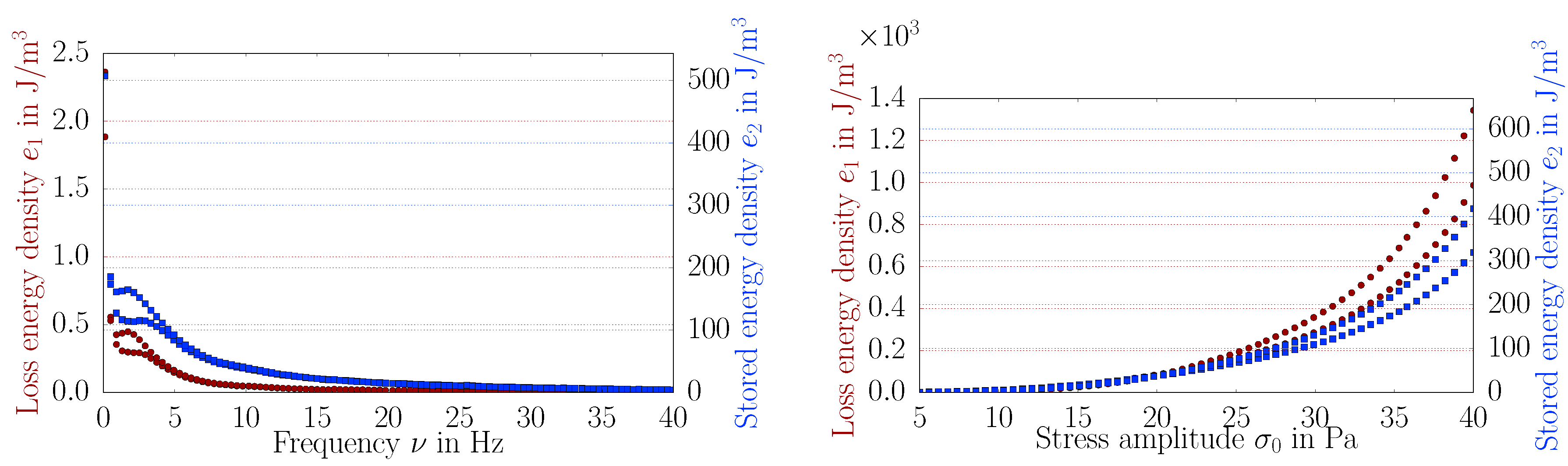
Figure 3.
Linear model, loss (red circles) and stored (blue squares) energies obtained from the measurement; corresponding fit curves as continuous lines. Left: Frequency variation by fixed amplitude, Pa. Right: Amplitude variation by fixed frequency, Hz.
Figure 3.
Linear model, loss (red circles) and stored (blue squares) energies obtained from the measurement; corresponding fit curves as continuous lines. Left: Frequency variation by fixed amplitude, Pa. Right: Amplitude variation by fixed frequency, Hz.
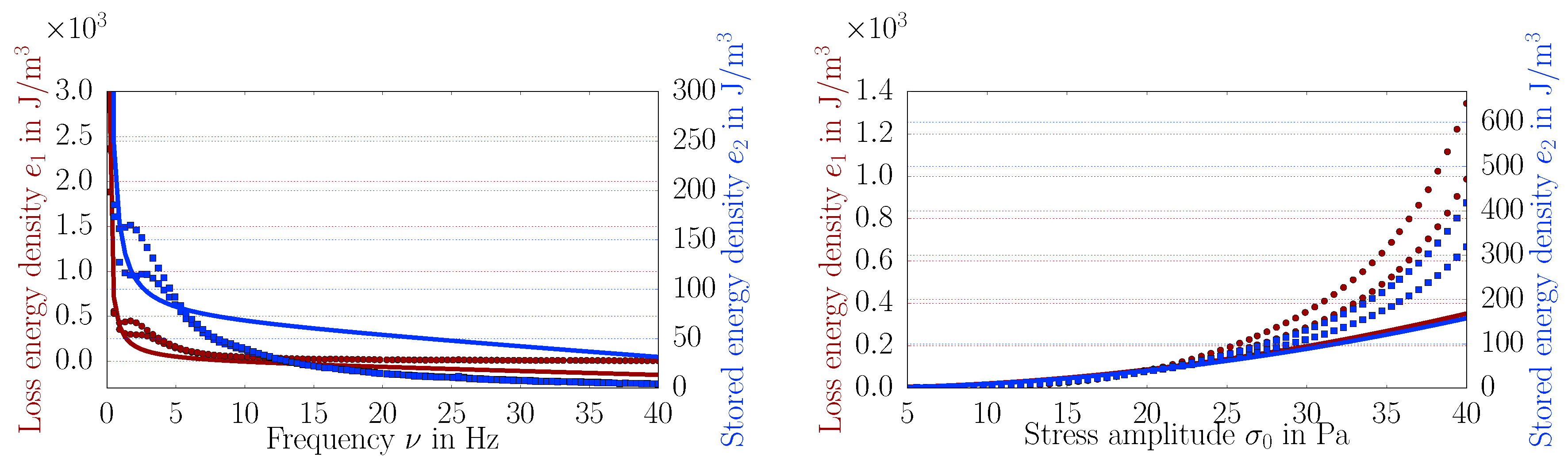
Figure 4.
Cubic model, loss (red circles) and stored (blue squares) energies obtained from the measurement; corresponding fit curves as continuous lines. Left: Frequency variation by fixed amplitude, Pa. Right: Amplitude variation by fixed frequency, Hz.
Figure 4.
Cubic model, loss (red circles) and stored (blue squares) energies obtained from the measurement; corresponding fit curves as continuous lines. Left: Frequency variation by fixed amplitude, Pa. Right: Amplitude variation by fixed frequency, Hz.

Figure 5.
Sigmoid model, loss (red circles) and stored (blue squares) energies obtained from the measurement; corresponding fit curves as continuous lines. Left: Frequency variation by fixed amplitude, Pa. Right: Amplitude variation by fixed frequency, Hz.
Figure 5.
Sigmoid model, loss (red circles) and stored (blue squares) energies obtained from the measurement; corresponding fit curves as continuous lines. Left: Frequency variation by fixed amplitude, Pa. Right: Amplitude variation by fixed frequency, Hz.

Figure 6.
Stress-strain plots with determined material parameters. Stress in the ordinate and strain in the abscissa in Lissajous–Bowditch plots for the linear (left) and sigmoid (right) models for different amplitudes and frequencies.
Figure 6.
Stress-strain plots with determined material parameters. Stress in the ordinate and strain in the abscissa in Lissajous–Bowditch plots for the linear (left) and sigmoid (right) models for different amplitudes and frequencies.
© 2018 by the author. Licensee MDPI, Basel, Switzerland. This article is an open access article distributed under the terms and conditions of the Creative Commons Attribution (CC BY) license (http://creativecommons.org/licenses/by/4.0/).
Share and Cite
MDPI and ACS Style
Abali, B.E. Inverse Analysis of Cellulose by Using the Energy-Based Method and a Rotational Rheometer. Appl. Sci. 2018, 8, 1354. https://doi.org/10.3390/app8081354
AMA Style
Abali BE. Inverse Analysis of Cellulose by Using the Energy-Based Method and a Rotational Rheometer. Applied Sciences. 2018; 8(8):1354. https://doi.org/10.3390/app8081354
Chicago/Turabian StyleAbali, Bilen Emek. 2018. "Inverse Analysis of Cellulose by Using the Energy-Based Method and a Rotational Rheometer" Applied Sciences 8, no. 8: 1354. https://doi.org/10.3390/app8081354
Note that from the first issue of 2016, this journal uses article numbers instead of page numbers. See further details here.