Image Dehazing and Enhancement Using Principal Component Analysis and Modified Haze Features


Department of Image, Graduate School of Advanced Imaging Science, Multimedia and Film, Chung-Ang University, Seoul 06974, Korea
*
Author to whom correspondence should be addressed.
†
These authors contributed equally to this work.
Appl. Sci. 2018, 8(8), 1321; https://doi.org/10.3390/app8081321
Submission received: 5 June 2018
/
Revised: 17 July 2018
/
Accepted: 24 July 2018
/
Published: 8 August 2018
(This article belongs to the Special Issue Advanced Intelligent Imaging Technology)
Abstract
:This paper presents a computationally efficient haze removal and image enhancement methods. The major contribution of the proposed research is two-fold: (i) an accurate atmospheric light estimation using principal component analysis, and (ii) learning-based transmission estimation. To reduce the computational cost, we impose a constraint on the candidate pixels to estimate the haze components in the sub-image. In addition, the proposed method extracts modified haze-relevant features to estimate an accurate transmission using random forest. Experimental results show that the proposed method can provide high-quality results with a significantly reduced computational load compared with existing methods. In addition, we demonstrate that the proposed method can significantly enhance the contrast of low-light images according to the assumption on the visual similarity between the inverted low-light and haze images.
1. Introduction
As various digital cameras are introduced in the consumer market with related multimedia services, the enhancement of outdoor hazy images attracts increasing interest. Haze occurs when the reflected light from an object is scattered or absorbed by the particles in the atmosphere and results in visibility degradation. In the case of vehicular systems, cameras should acquire as clean of an image as possible, even in bad weather, including hazy and rainy conditions. Since the haze particles limit the performance of the recognition of other vehicles, pedestrian, and traffic signs, haze removal should be performed in the consumer devices to obtain high-quality images. In addition, hazy images lose color information and contrast because of the haze component. To challenge this problem, various haze removal methods have been proposed in the literature. He et al. proposed a haze removal method using the dark channel prior (DCP) which consists of the minimum brightness value among the red (R), green (G), and blue (B) pixels in the local image patch [1]. The DCP plays an important role in estimating the transmission and atmospheric light to remove the haze component. However, He’s method exhibits inaccurately estimated atmospheric light, especially in the bright region. Moreover, it is not easy to implement the method in consumer devices because of the high computational complexity in refining the transmission. To solve this problem, Zhu et al. proposed a linear model to estimate the depth using the color attenuation prior which represents the relationship between the brightness and saturation components of hazy images [2]. Ancuti et al. estimated the hazy region by estimating the differences between hue components in the hazy image and its semi-inverse [3].
Learning-based haze removal methods were also proposed using haze-relevant features. Tang et al. proposed a haze estimation method by learning a regression model using random forest [4]. Tang’s method can provide better results than existing methods at the cost of an increasing computational load to extract features in overlapping patches. Deep convolutional neural network-based haze removal methods have also been proposed to estimate more accurate transmission information [5,6]. However, their performance is also limited since transmission and atmospheric light cannot be learned simultaneously.
Recently, Fattal et al. proposed a haze removal method based on the assumption that pixels having the same color in the haze region lie on the same line in the RGB color space [7]. Although this method uses a local image formation model to estimate the accurate transmission, it provides an over-dehazed result according to the light condition. Berman et al. defined a haze-line based on the observation that haze-free images can be expressed by a finite number of color values [8]. In hazy images, clustered pixels using k-means in haze-free images are distributed along the haze-lines. In order to estimate an optimal solution, Meng et al. proposed a haze removal method by performing contextual regularization using a bounded constraint and weighted -norm [9]. In addition, He et al. estimated haze removal using convex optimization based on the discrete Haar wavelet transform to reduce the computational cost [10].
On the other hand, Sulami et al. estimated the optimal atmospheric light based on a new geometry assumption in the RGB vector space [11]. This method assumes that the principal component vectors of all the patches in a haze-free image are through the origin of the RGB vector space. However, since the haze component is added to the patch’s principal component vector, it cannot be passed through the origin. For that reason, this method estimates the vector of an atmospheric light using a principal component analysis (PCA) of the image patches. However, since this method selects the image patch including the candidate pixel of atmospheric light at every pixel, it provides the resulting image at a high-computational cost.
Yoon et al. extracted the sky region and estimated transmission using color correction in the HSV color space [12]. Kim et al. improved surveillance monitoring images using a DCP-based maximum filter to remove the haze components [13]. Kim et al. also performed haze removal using the disparity map which was estimated between a set of stereo images [14].
To solve this problem, this paper presents a novel estimation method for the optimal atmospheric light and the transmission. The contribution of the proposed method is two-fold: (i) estimation of atmospheric light vectors using the reduced pixels based on the PCA, and (ii) estimation of the transmission component using random forest via modified haze-relevant features. Since the atmospheric light is estimated by constraining the searching region and clustering the similar pixels to reduce the candidate pixels, the computational complexity is significantly reduced. In addition, the proposed method estimates the transmission using single-scale haze-relevant features to simplify the random forest. In conclusion, the proposed method can provide similar results at a low computational cost.
This paper is organized as follows. Section 2 describes the modified haze removal model as the theoretical background. Section 3 presents the proposed haze removal method using optimal atmospheric light and transmission in detail. Experimental results are shown in Section 4, and Section 5 concludes the paper.
2. Theoretical Background
Degradation Model of a Haze Image
In the hazy condition, the light scattered by various types of particles in the atmosphere decreases the visibility of the acquired image. In addition, the amount of image degradation is proportional to the distance between the object and camera. He et al. proposed the transmission-based haze removal method in reference [1], where the image degradation model is defined as
where represents the observed hazy image; is the haze-free image; A is the atmospheric light; and is the transmission. The transmission () is defined as
where represents the scattering coefficient of the atmosphere, and is the scene depth.
He et al. analyzed the statistical properties of various haze-free images based on a histogram. They introduced the DCP which is estimated by selecting the minimum intensity value among the R, G, and B pixels. In this method, the haze-free image is obtained by solving the degradation model using properly estimated A and values. The haze-free image was obtained as
If A and are inaccurately estimated, color distortion and brightness saturation many occur in the resulting image.
On the other hand, Sulami et al. presented the localized haze model using a small patch in a hazy image in reference [11], where the image degradation model is defined as
where represents the i-th patch in ; is the i-th patch in the transmission; is the RGB vector representing the reflected light from ; and a constant magnitude of the A. This model assumes that the vectors of the principal component of the patches in a haze image intersect the vector of atmospheric light, which passes through the origin in the RGB color space. Sulami et al. estimated the orientation and magnitude of the atmospheric light vector using the PCA of the selected haze patch satisfying the degradation model of (4) [11].
3. Haze Removal Using PCA and Haze-Relevant Features
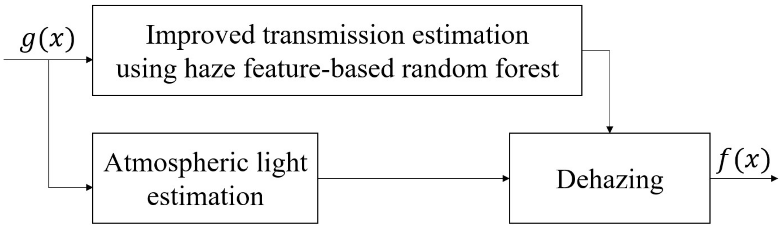
The proposed method consists of two steps: (i) atmospheric light estimation using PCA, and (ii) transmission estimation using modified haze-features and random forest. An additional contribution of the proposed dehazing algorithm is its computational efficiency that can significantly reduce the processing time and computation resources, particularly for consumer mobile cameras. Figure 1 shows the block diagram of the proposed method.
3.1. Estimation of the Atmospheric Light Using PCA
Since existing dehazing methods estimate the atmospheric light for every candidate pixel in the input haze image, they require a very large amount of computation. To solve this problem, the proposed method estimates the atmospheric light vector using PCA on the the reduced number of the candidate haze patches.
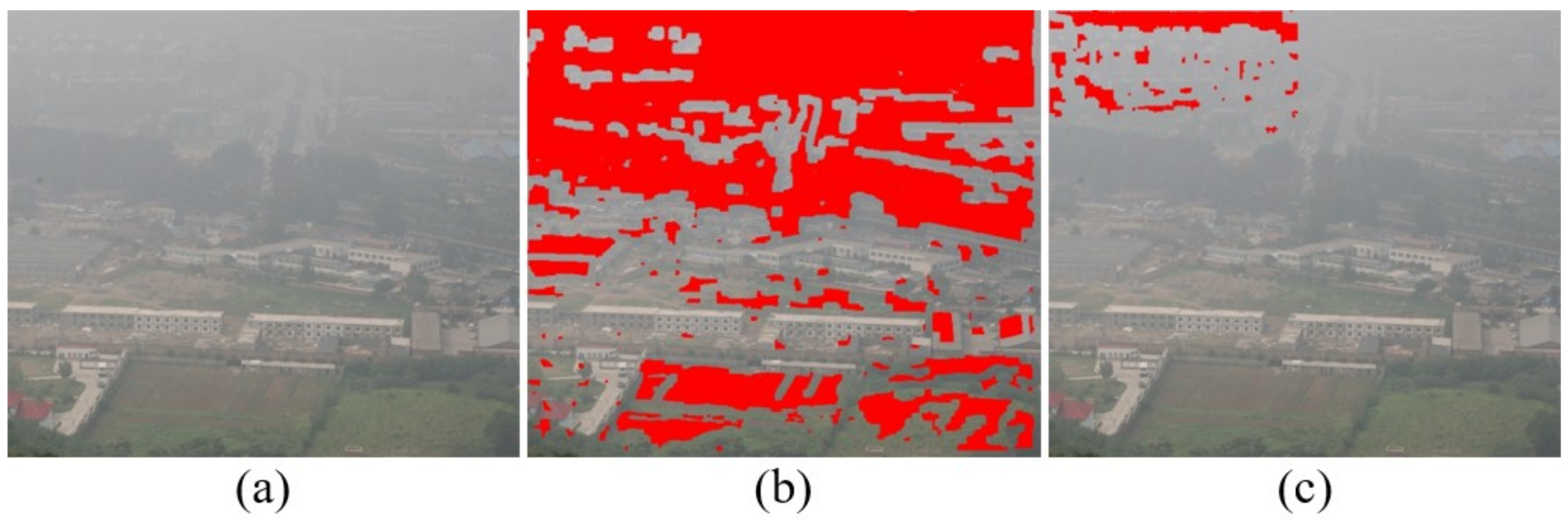
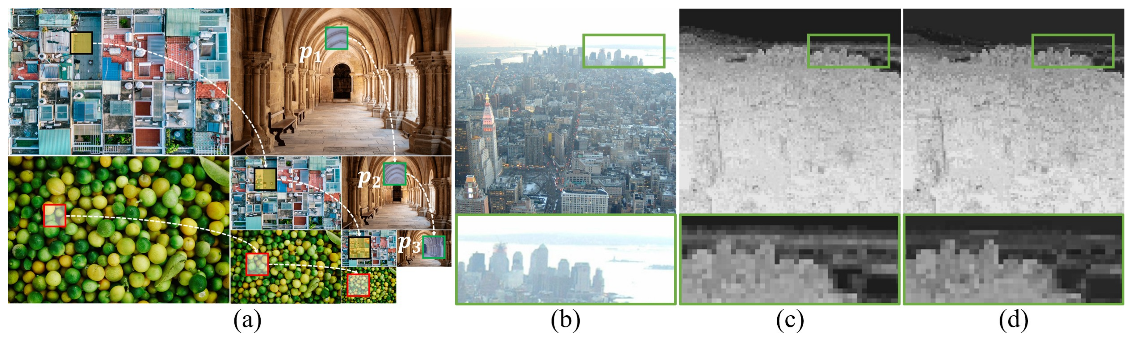
Sulami et al. estimated the atmospheric light by estimating the intersection of the principal vectors of the haze patches, but they performed PCA twice on all haze patches, which requires more computation [11]. In the proposed method, we employ the additional constraints to efficiently estimate the atmospheric light using the reduced number of the candidate pixels regarded as haze particles, as shown in Figure 2.
More specifically, the proposed method reduces the number of candidate haze patches by dividing the input image into four sub-images and then selects the sub-image with the maximum mean brightness value. Since the haze region smoothly varies with the bright pixels, we assume that the selected sub-image with the maximum average includes more haze components. Figure 2 shows the comparison of the region of interests containing the candidate atmospheric light to be estimated.
In addition, the proposed method can reduce the probability of inaccurate estimation which regards a bright object as the atmospheric light, since the region of maximum average in the image is usually the sky area. For that reason, the proposed method selects the non-edge candidate pixels that have higher intensity values than the average of the selected sub-image, as shown in Figure 2c. As a result, the proposed method can estimate the candidate atmospheric light at the reduced processing time, because the candidate region is selected, providing the highest mean brightness value.
Since the haze patch containing the haze pixel smoothly varies with similar intensity values and principal vector, Sulami et al. proposed constraints to select a haze patch having the positive principal component, a single large eigenvalue, and a PCA matrix of rank-one [11]. However, since Sulami et al. performed PCA twice to remove outliers by discarding the farthest principal component vector, this method requires more computation. On the other hand, the proposed method can estimate the atmospheric light vector using the constraints proposed in reference [11] in a computationally efficient manner, because the constraints of the proposed method reduce the number of haze patches to be computed.
The optimum haze patches containing the atmospheric light are selected at the intersection of the principal component vectors. The candidate vector of atmospheric light is determined to give the smallest error among the intersection points and principal vectors of the optimum haze patches. For that reason, the magnitude of atmospheric light of a hazy image can be estimated using the candidate vectors as
where represents the i-th candidate vector of the atmospheric light. Since the magnitude of the atmospheric light is estimated by averaging the magnitude of , the proposed method can provide more accurate atmospheric light in a haze image.
Figure 3 shows the dehazing results using the atmospheric light values estimated by three different haze removal methods, including the proposed method. The dehazing results were obtained by solving the degradation model of a hazy image in (3). In experiments, we differently estimated the atmospheric light using existing and proposed methods, and the transmission was obtained using He’s method [1] as
where
represents the transmission; is the positive constant parameter; is the dark channel at the local window of size whose center is located at x; and is the the region of the local window. Since the transmission is estimated by inverting the normalized and weighted DCPs, it can be regarded that the DCP approximately represents the quantity of haze components [1].
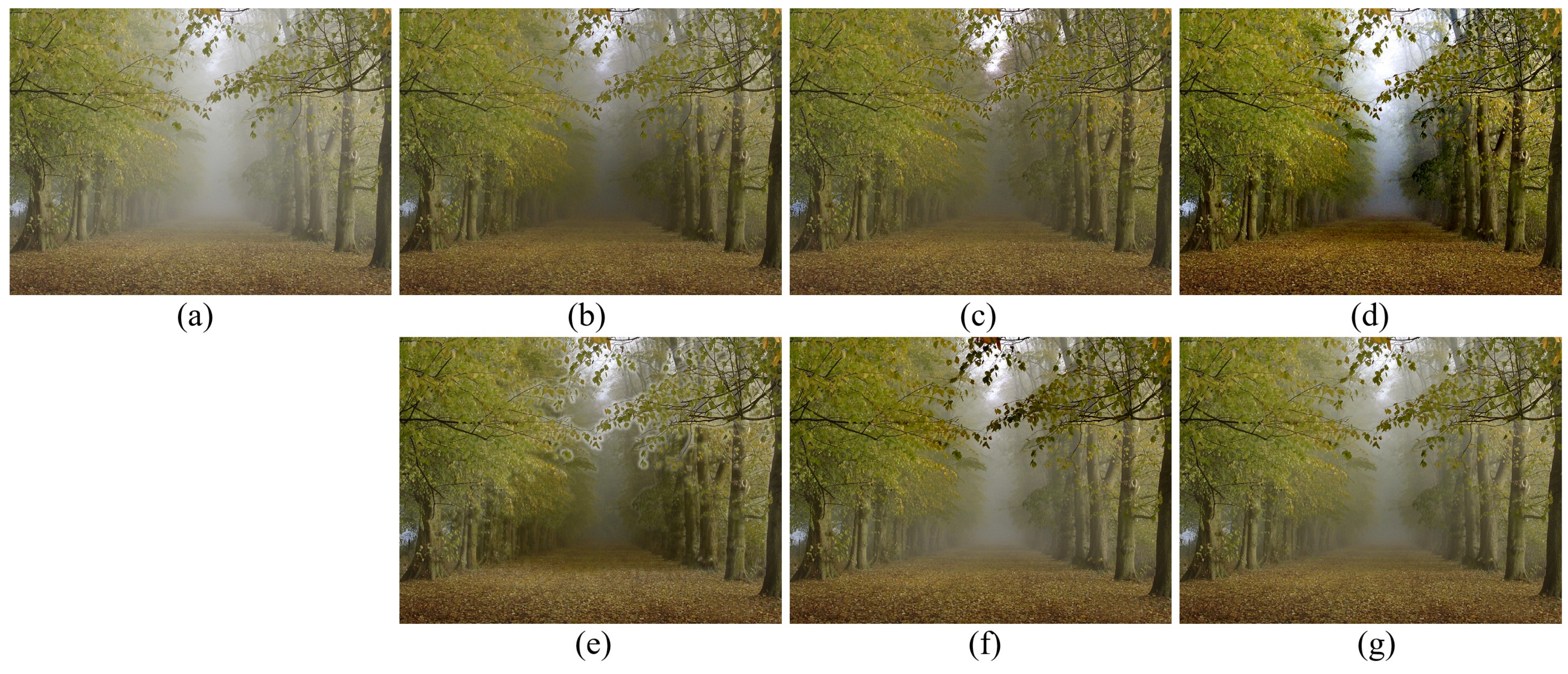
Figure 3a shows the ground-truth of an atmospheric light and input haze image. Since Sulami’s method estimated darker atmospheric light than the ground-truth, the resulting image shows brightness saturation in the sky region, as shown in Figure 3b. Berman’s method produces color distortion because the color of the estimated atmospheric light is different from that of the ground-truth [15]. On the other hand, the proposed method accurately estimated atmospheric light similarly to the ground-truth, and as a result, it can remove the haze without brightness saturation or color distortion.
3.2. Transmission Estimation Using Random Forest
In this sub-section, we describe the haze-relevant features to accurately estimate the transmission. Tang et al. estimated the haze-relevant features from thirteen differently scaled spaces at the cost of a high computational overhead [4]. On the other hand, the proposed method extracts the haze-relevant features of the dark channel and local contrast in a single in-scale haze image. The haze components decrease the contrast of an input image by scattering the light in the atmosphere. For that reason, the proposed method uses the local maximum contrast to train the random forest, which estimates the contrast enhanced transmission. The local maximum contrast is defined as
where represents the neighborhood region with center x. The local maximum contrast feature represents the variance between the center and the surrounding pixels in the patch.
The haze-relevant features to train the random forest are extracted from the synthesized haze patches based on (1) [4]. The model to synthesize a haze patch is defined as
where represents the synthesized hazy patch; is the haze-free patch; and is the range of transmission. The haze-relevant features of dark channel and local maximum contrast extracted from synthesized haze patches are used as the training data in the random forest. However, if an object is close to the camera, the light ray travels through less particles which results in a high transmission value. In addition, since a very high transmission value results in over-dehazing, the correspondingly dehazed region looks unnatural [1]. For that reason, we constrained the range of transmission from 0.1 to 0.9 to synthesize the haze patch.
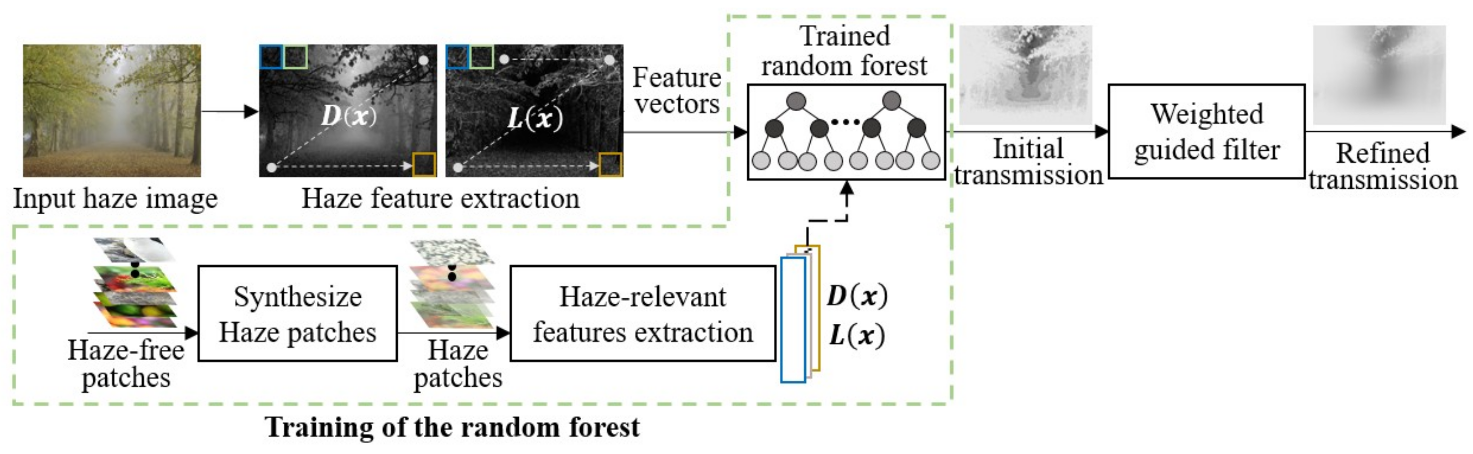
The color vector of the atmospheric light in a synthesized patch is supposed to be , since the synthesized patch cannot adaptively estimate A for each patch. To solve this problem, the proposed method performs normalization by estimating the atmospheric light on the haze image to prevent brightness saturation. Moreover, the estimated transmission tends to result in a blocking artifact, because the transmission is estimated using the random forest with the haze-relevant features in a patch-wise manner. For that reason, the proposed method uses weighted guided filtering to refine the initial transmission [17]. Figure 4 shows the transmission estimation using the proposed haze-relevant features and random forest and the training of random forest using the haze-relevant features extracted from the synthesized haze patches. In this work, we used 100 decision trees for the random forest.
In the random forest regression process, selection of good features can reduce the training time [18]. Figure 5 shows that the number of haze-relevant features used in the proposed method is related to the prediction of the transmission compared with existing method. We used the quantity ‘importance’ as a measure of each feature based on the variation of out-of-bag (OOB) error, which means that it is averaged and divided by the standard deviation over the all trees [4]. The multiscale dark channel and local contrast features, denoted by and in Figure 4, respectively, have significantly different importance values, as shown in Figure 5. It can be seen from the feature importance that the features on a certain scale do not have a significant effect on the learning-based prediction results. On the other hand, the importance of the proposed method is higher than that of the existing method which means that the haze features of the proposed method are more related to the transmission estimation than the existing features.
3.3. Training the Random Forest
The proposed method used a set of high-resolution haze-free images collected from the internet to generate the training dataset for the learning of random forest [19]. In the proposed method, the random forest is trained using the haze-relevant features of the local maximum contrast and dark channel. However, since the local maximum contrast and dark channel features are more salient in the non-sky region, we extracted the haze-free patches from non-sky regions. In addition, since it is hard to obtain the transmission of observed haze image directly, we synthesized haze patches using transmission values from 0.1 to 0.9 based on the patch-based haze model in (9). We generated 10,000 pairs of haze and haze-free patches for each t and extracted the haze-relevant features to train the random forest. Eighty percent of the training dataset was used for training and the rest was used for testing for each t in (9).
In addition, we extracted the haze-free patches from a set of image pyramid to generate a pair of haze and haze-free patches, as shown in Figure 6a. Since transmission is constant at regions of the same depth, the transmissions of patches , , and extracted at in- and across-scales should also be constant. For that reason, multiscaled patches of the same size can be regarded as a set of different scenes at the same depth. Figure 6c,d respectively show the comparison of estimated transmissions using random forest.
Figure 6c is the transmission estimated using the random forest trained by the haze-relevant features estimated from the haze patches, which were synthesized using haze-free patches extracted from a single in-scale space. On the other hand, the random forest used in Figure 6d was trained using the haze-relevant features estimated from the haze patches, which were synthesized using haze-free patches extracted from multiscaled spaces. As shown in Figure 6d, the haze-free patches extracted from multiscale spaces are more related to the relationship between the haze-relevant features and transmission compared with Figure 6c. For that reason, the proposed method can estimate a more accurate transmission at the same scene depth from an image pyramid and random forest.
4. Experimental Results
This section demonstrates the performance of the proposed haze removal method using existing dehazing methods proposed by He et al. [1], Meng et al. [9], Berman et al. [8,15], Zhu et al. [2], Ren et al. [6], and Sulami et al. [11]. The performances of haze removal methods were compared in terms of atmospheric light estimation, dehazing, and processing time. Objective quality assessments were performed using the -error of the estimated atmospheric light and visibility level descriptor proposed in reference [20,21]. To evaluate the processing time, we performed the experiments using a personal computer equipped with 3.70 GHz CPU with six cores and 48 GByte of RAM. The proposed method was implemented using Matlab and the Parallel Computing Toolbox.
4.1. Comparison of the Estimated Atmospheric Light
This subsection demonstrates the performance of the atmospheric light estimation using a pair of 34 haze and ground-truth images proposed in reference [20]. Bahat et al. manually extracted the specified region of the ground-truth atmospheric light. Objective assessments are summarized in Table 1. Figure 7 shows estimated atmospheric lights using the existing and proposed methods given the ground-truth of atmospheric light.
Since He’s method estimated the atmospheric light using the top 0.1% brightest pixels of the DCP, the estimated atmospheric light may be inaccurate because of the brightest object in a haze image [1]. As shown in Figure 7c, Sulami’s method provided darker atmospheric light because this method does not compensate the magnitude of the atmospheric light vector when estimating the atmospheric light [11]. Berman’s method estimated the atmospheric light located at the end of the haze-line [15]. For that reason, the Berman’s method showed a bright atmospheric light value, as shown Figure 7d.
On the other hand, since the proposed method estimates the atmospheric light using the candidate pixels in a specified region, the estimated atmospheric light should be similar to the ground-truth. Table 1 shows that the proposed method provided the lowest -error in terms of the atmospheric light estimation compared with existing methods. In terms of the processing time, the proposed method provided the best and second best processing times with and without parallel processing, respectively.
4.2. Objective Assessments
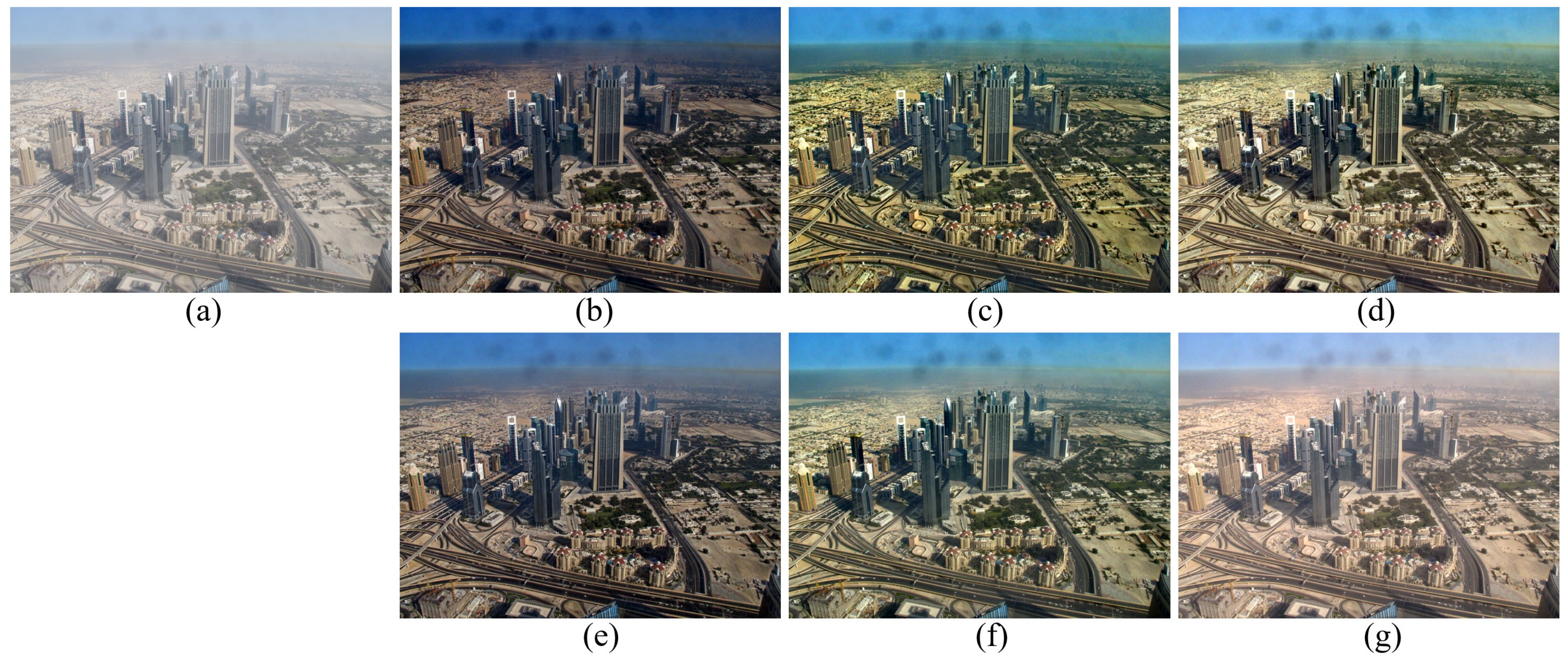
Figures 9–11 compare the performance of the haze removal using the existing and proposed methods. The objective assessments were performed using Hautiere’s method and a set of test images, which were presented in He’, Tang’, Liu’s, and Cai’s works, as shown in Figure 8 [1,4,5,16]. and respectively represent the ratios of brightest and darkest pixels and the ratio of gradient norms between the input and haze-removed images [21]. The small value of means that the resulting image has a lower brightness saturation while preserving the dark region. On the other hand, if is close to 1, the gradient of the resulting image does not change without over-dehazing [22]. The objective assessments are summarized in Table 2.
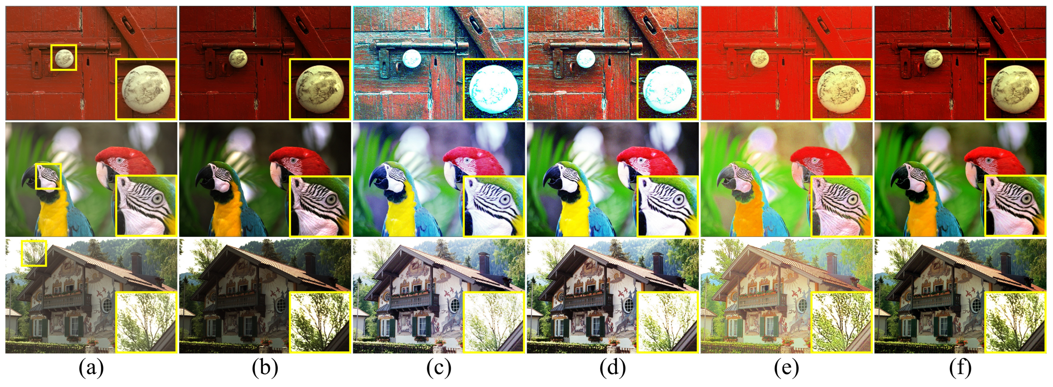
As shown in Figure 9b, Figure 10b and Figure 11b, He’s method provided an enhanced result in the sense that it preserved the details in the dark and bright regions with the best score of [1]. Although Meng’s method provided improved results using -norm minimization, it could not avoid saturation in the bright region, as shown in Figurs Figure 9c, Figure 10c and Figure 11c [9] . Since Berman’s method reduced the haze component based on the haze-line, it was able to preserve the color information, as shown in Figure 9d, Figure 10d and Figure 11d [8]. However, it is difficult to choose an appropriate parameter to obtain the optimal result and the resulting images include brightness saturation.
Figure 9e, Figure 10e and Figure 11e show the resulting images fromusing Zhu’s method with the halo effect near the edges [2]. Although Ren’s method estimated the transmission using the convolutional neural network, the resulting images show color distortion because of the inaccurately estimated atmospheric light [6]. On the other hand, the proposed method provided better results than most existing methods with improved contrast and lower brightness saturation.
Since Tang et al. used the random forest of 200 decision trees with multiscaled haze features to solve the regression problem [4], their algorithm took about 193.9253 and 99.9524 s for feature extraction and the learning of random forest, respectively, for an input image of size 3873 × 2516, as shown in Figure 12a. On the other hand, since the proposed method divides the input image into 5 × 5 non-overlapping patches to extract the haze features, it took only about 9.7474 and 25.6829 s with and without parallel processing for feature extraction, respectively. The estimation of transmission using the trained random forest took about 17.0358 s with 100 decision trees. In addition, the proposed method was able to provide similar MSE values with a smaller number of decision trees for the random forest, as summarized in Table 3.
Table 3 shows the comparative results for the mean squared error (MSE) of the estimation of transmission using synthesized outdoor haze images. Figure 12 is a set of original haze-free images that were used to synthesize haze patches to estimate MSE values in reference [23]. As summarized in Table 3, the proposed method provided lower MSE scores than Tang’s method [4]. This means that the proposed method can estimate more accurate atmospheric light and transmission with a significantly reduced computational load regardless of the number of trees.
4.3. Application to Low-Light Image Enhancement
In this subsection, we demonstrate that the proposed method can improve the quality of a low-light image by using the degradation model of an inverted haze image. Dong et al. assumed that inverted low-light images are similar to hazy images by analyzing a histogram [24]. Jiang et al. showed that an inverted low-light image can be regarded as a haze image in terms of visual similarity [25].
Based on this observation, they improved the quality of low-light images by solving the degradation model of a haze image with an inverted low-light image. The conventional haze model in (1) can be rewritten by respectively substituting and with their inverted versions:
where and respectively represent the inverted versions of the input low-light and the latent images. To enhance the brightness of an input low-light image, Jiang et al. estimated the transmission using the dark channel prior and obtained the latent image by solving the degradation model in (3) by
In the proposed method, we estimated the atmospheric light using the proposed method described in Section 3. The transmission of the inverted low-light image is estimated by using the trained random forest with dark channel and local contrast features. To evaluate the performance of the low-light image enhancement, we synthesized the low-light image by the non-linear gamma correction using a set of test images as shown in Figure 13. The adjustment parameter was set to 2.5.
Figure 14 compares the objective performance of the low-light image enhancement using the existing and proposed methods. The first and second columns respectively show a set of ideal and synthesized low-light images. As shown in Figure 14c, the resulting image of the histogram equalization (HE) shows both over-enhancement and color distortion, because the cumulative distribution function is drastically changed in the narrow region [26].
Huang et al. presented the gamma correction-based image enhancement method using the weighted cumulative distribution function [27]. However, Huang’s method generated brightness saturation in the bright region, as shown in Figure 14d. Jiang’s method provided a significantly enhanced result, but it could not avoid color distortion in the resulting image, as shown in Figure 14e [25]. On the other hand, the proposed method provided better results than most existing methods without brightness saturation and color distortion, as shown in Figure 14f. Table 4 shows the objective assessments using the peak signal-to-noise ratio (PSNR) and structural similarity index measure (SSIM) [28].
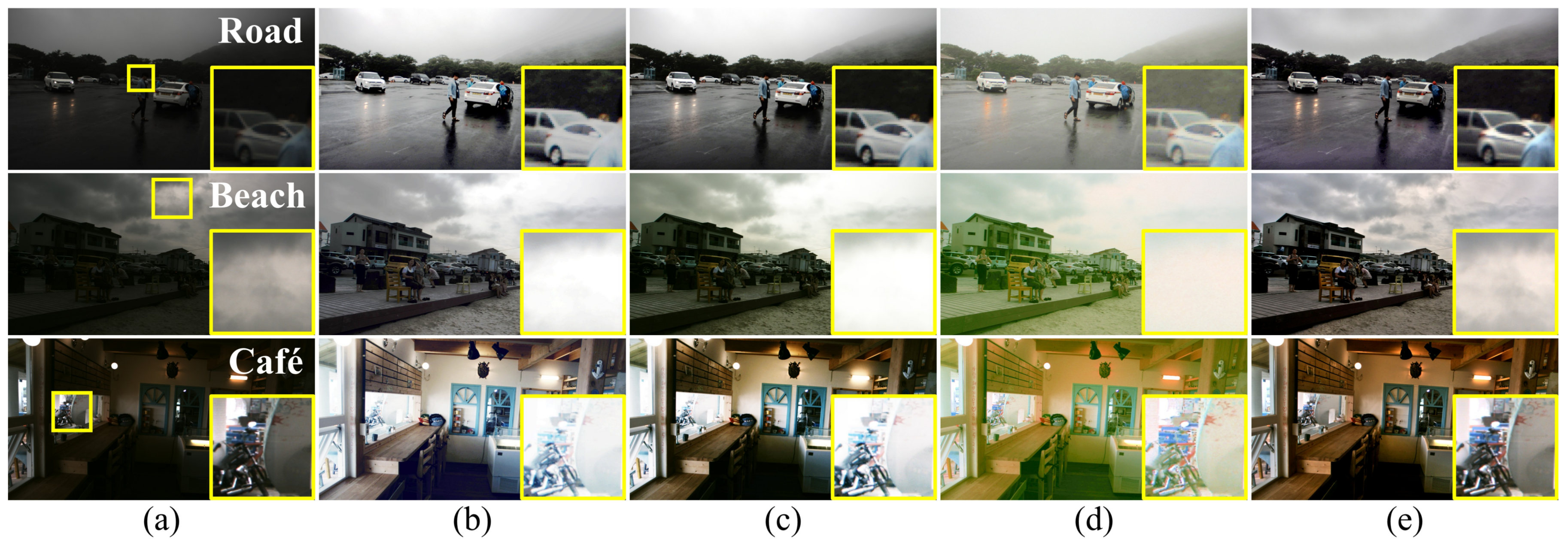
Figure 15 shows the resulting images of the low-light image enhancement using real low-light images. The HE shows the contrasting enhanced result, but it did not preserve the details in the bright region, as shown in Figure 15b [26]. Huang’s method provided a more enhanced result than that of HE [27]. However, the resulting image could neither appropriately control the brightness saturation, nor successfully enhance the dark region, as shown in Figure 15c. In the same manner, Jiang’s method also provided the resulting image with brightness saturation, and it showed imbalanced amplification of the color components, as shown in Figure 15d [25].
On the other hand, the proposed method provided the resulting image with an increased dynamic range, preserving the details of the bright region without color distortion. Table 5 shows objective assessments using the autoregressive-based image sharpness metric (ARISM), which evaluates the sharpness ratio by analyzing the autoregressive image model without reference images [30]. We used the ARISM as a metric to evaluate the amount of detail in the bright and dark regions. As summarized in Table 5, Although the HE provided the best score, the proposed method provided better visual quality, as shown Figure 15.
5. Conclusions
This paper presented haze removal and low-light image enhancement methods using the supervised learning manner. The proposed method simplifies the atmospheric light estimation using the feature of haze patches analyzed by the principal component analysis. To estimate an accurate transmission, we generated the synthesized haze patches using the haze-free patches extracted from the non-hazy region at multiscaled spaces. The transmission was estimated in a supervised learning manner using random forest with two haze-relevant features. Through experiments, we demonstrated that the proposed method can estimate accurate atmospheric light and transmission than existing haze removal methods. As a result, the proposed method can obtain the resulting image without color distortion or brightness saturation. In addition, we demonstrated that the proposed method can be applied to low-light image enhancement problems using the degradation model of an inverted haze image. In conclusion, the proposed method can provide high-quality images for various image processing applications in haze and low-light conditions.
Author Contributions
M.K and S.Y. initiated the research and designed the experiments. S.P. acquired the test images and performed the experiments. S.L. analyzed the experimental results and J.P. wrote the manuscript.
Funding
This work was partly supported by Institute for Information & Communications Technology Promotion(IITP) Grant, funded by the Korean Government (MSIT) (2017-0-00250, Intelligent Defense Boundary Surveillance Technology Using Collaborative Reinforced Learning of Embedded Edge Camera and Image Analysis), and by the Korea Aerospace Research Institute (NRF-2017M1A3A4A07028434).
Conflicts of Interest
The authors declare no conflicts of interest.
References
- He, K.; Sun, J.; Tang, X. Single image haze removal using dark channel prior. IEEE Trans. Pattern Anal. Mach. Intell. 2011, 33, 2341–2353. [Google Scholar] [PubMed]
- Zhu, Q.; Mai, J.; Shao, L. A Fast single image haze removal algorithm using color attenuation prior. IEEE Trans. Image Process. 2015, 24, 3522–3533. [Google Scholar] [PubMed]
- Ancuti, O.; Ancuti, C.; Hermans, C.; Bekaert, P. A fast semi-inverse approach to detect and remove the haze from a single image. In Proceedings of the Asian Conference on Computer Vision, Queenstown, New Zealand, 8–12 November 2010; pp. 501–514. [Google Scholar]
- Tang, K.; Yang, J.; Wang, J. Investigating haze-relevant features in a learning framework for image dehazing. In Proceedings of the IEEE Conference on Computer Vision and Pattern Recognition, Columbus, OH, USA, 24–27 June 2014; pp. 2995–3002. [Google Scholar]
- Cai, B.; Xu, X.; Jia, K.; Qing, C.; Tao, D. DehazeNet: An end-to-end system for single image haze removal. IEEE Trans. Image Process. 2016, 25, 5187–5198. [Google Scholar] [CrossRef] [PubMed]
- Ren, W.; Liu, S.; Zhang, H.; Pan, J.; Cao, X.; Yang, M. Single image dehazing via multi-scale convolutional neural networks. In Proceedings of the European Conference on Computer Vision, Amsterdam, The Netherlands, 8–16 October 2016; pp. 154–169. [Google Scholar]
- Fattal, R. Dehazing using color-lines. ACM Trans. Graph. 2014, 34, 13. [Google Scholar] [CrossRef]
- Berman, D.; Treibitz, T.; Avidan, S. Non-local image dehazing. In Proceedings of the IEEE Conference on Computer Vision and Pattern Recognition, Las Vegas, NV, USA, 27–30 June 2016; pp. 1674–1682. [Google Scholar]
- Meng, G.; Wang, Y.; Duan, J.; Xiang, S.; Pan, C. Efficient image dehazing with boundary constraint and contextual regularization. In Proceedings of the IEEE Conference on Computer Vision, Darling Harbour, Sydney, Australia, 3–6 December 2013; pp. 617–624. [Google Scholar]
- He, J.; Zhang, C.; Yang, R.; Zhu, K. Convex optimization for fast image dehazing. In Proceedings of the IEEE Conference on Image Processing, Phoenix, AZ, USA, 25–28 September 2016; pp. 2246–2250. [Google Scholar]
- Sulami, M.; Glatzer, I.; Fattal, R.; Werman, M. Automatic recovery of the atmospheric light in hazy images. In Proceedings of the IEEE International Conference Computer Photography, Santa Clara, CA, USA, 2–4 May 2014; pp. 1–11. [Google Scholar]
- Yoon, I.; Kim, S.; Kim, D.; Hayes, M.H.; Paik, J. Adaptive defogging with color correction in the HSV color space for consumer surveillance system. IEEE Trans. Consum. Electron. 2012, 58, 111–116. [Google Scholar] [CrossRef]
- Kim, W.; Bae, H.; Kim, T. Fast and efficient haze removal. In Proceedings of the IEEE International Conference Consumer Electronics, Las Vegas, NV, USA, 9–12 January 2015; pp. 360–361. [Google Scholar]
- Kim, H.; Park, J.; Park, H.; Paik, J. Iterative refinement of transmission map for stereo image defogging. In Proceedings of the IEEE International Conference Consumer Electronics, Las Vegas, NV, USA, 8–11 January 2017; pp. 296–297. [Google Scholar]
- Berman, D.; Treibitz, T.; Avidan, S. Air-light estimation using haze-lines. In Proceedings of the IEEE International Conference on Computer Photography, Palo Alto, CA, USA, 12–14 May 2017; pp. 1–9. [Google Scholar]
- Liu, P.J.; Horng, S.J.; Lin, J.S.; Li, T. Contrast in haze removal: configurable contrast enhancement model based on dark channel prior. IEEE Trans. Image Process. 2018. [Google Scholar] [CrossRef] [PubMed]
- Li, Z.; Zheng, Z.; Zhu, Z.; Yao, W.; Wu, S. Weighted guided image filtering. IEEE Trans. Image Process. 2015, 24, 120–129. [Google Scholar] [PubMed]
- Kim, K.; Kim, S.; Sohn, K. Lazy dragging: Effortless bounding-box drawing for touch-screen devices. IEEE Trans. Consum. Electron. 2017, 63, 93–100. [Google Scholar] [CrossRef]
- Unsplash. Available online: https://unsplash.com/ (accessed on 31 July 2018).
- Bahat, Y.; Irani, M. Blind dehazing using internal patch recurrence. In Proceedings of the IEEE International Conference on Computer Photography, Evanston, IL, USA, 13–15 May 2016; pp. 1–9. [Google Scholar]
- Hautiere, N.; Tarel, J.P.; Aubert, D.; Dumont, E. Blind contrast enhancement assessment by gradient ratioing at visible edges. Image Anal. Stereol. 2011, 27, 87–95. [Google Scholar] [CrossRef]
- Ancuti, O.; Ancuti, C. Single image dehazing by multi-scale fusion. IEEE Trans. Image Process. 2013, 22, 3271–3282. [Google Scholar] [CrossRef] [PubMed]
- Zhang, Y.; Ding, L.; Sharma, G. HazeRD: An outdoor scene dataset and benchmark for single image dehazing. In Proceedings of the IEEE International Conference on Image Processing, Beijing, China, 17–20 September 2017; pp. 3205–3209. [Google Scholar]
- Dong, X.; Wang, G.; Pang, Y.; Li, W.; Wen, J.; Meng, W.; Lu, Y. Fast efficient algorithm for enhancement of low lighting video. In Proceedings of the IEEE International Conference on Multimedia and Expo, Barcelona, Spain, 11–15 July 2011; pp. 1–6. [Google Scholar]
- Jiang, X.; Yao, H.; Zhang, S.; Lu, X.; Zeng, W. Night video enhancement using improved dark channel prior. In Proceedings of the IEEE International Conference on Image Processing, Melbourne, Australia, 15–18 September 2013; pp. 553–557. [Google Scholar]
- Gonzalez, R.C.; Woods, R.E. Digital Image Processing, 3rd ed.; Prentice-Hall: Upper Saddle River, NJ, USA, 2007. [Google Scholar]
- Huang, S.C.; Cheng, F.C.; Chiu, Y.S. Efficient contrast enhancement using adaptive gamma correction with weighting distribution. IEEE Trans. Image Process. 2013, 22, 1032–1041. [Google Scholar] [CrossRef] [PubMed]
- Wang, Z.; Bovik, A.; Sheikh, H.; Simoncelli, E. Image quality assessment: From error visibility to structural similarity. IEEE Trans. Image Process. 2004, 13, 600–612. [Google Scholar] [CrossRef] [PubMed]
- Kodak Lossless True Color Image Suite. Available online: http://r0k.us/graphics/kodak/ (accessed on 31 July 2018).
- Gu, K.; Zhai, G.; Lin, W.; Yang, X.; Zhang, W. No-reference image sharpness assessment in autoregressive parameter space. IEEE Trans. Image Process. 2015, 24, 3218–3231. [Google Scholar] [PubMed]
Figure 1.
The block diagram of the proposed method.

Figure 2.
Region of interests for the candidate atmospheric light pixels: (a) input hazy image [11], reproduced with permission from [11], IEEE, 2014, (b) Sulami’s method [11], and (c) the proposed method.

Figure 3.
Comparative results of the atmospheric light estimation to remove haze. The top row shows the estimated atmospheric light using existing and proposed methods. The second row shows dehazed images using (3) and estimated atmospheric light of the top row: (a) input haze image [16], reproduced with permission from [16], IEEE, 1969 (b) Sulami’s method [11], (c) Berman’s method [15], and (d) the proposed method.
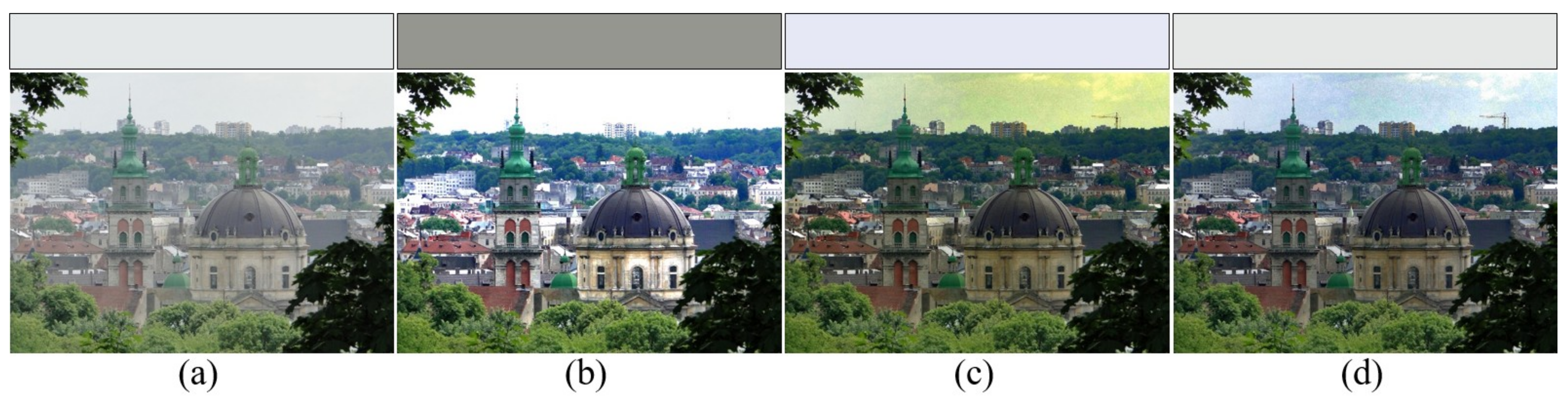
Figure 4.
The proposed transmission estimation process using haze-relevant features and random forest. The green dash line shows the training of the random forest using the haze-relevant features extracted from the synthesized haze patches. In the haze feature extraction block, and represent the dark channel and local contrast, respectively.

Figure 5.
Comparison of the importance rate of each haze feature by random forest regression. The solid line represents the importance rate of the proposed method and the dotted line shows that of Tang’s method [4].
Figure 5.
Comparison of the importance rate of each haze feature by random forest regression. The solid line represents the importance rate of the proposed method and the dotted line shows that of Tang’s method [4].
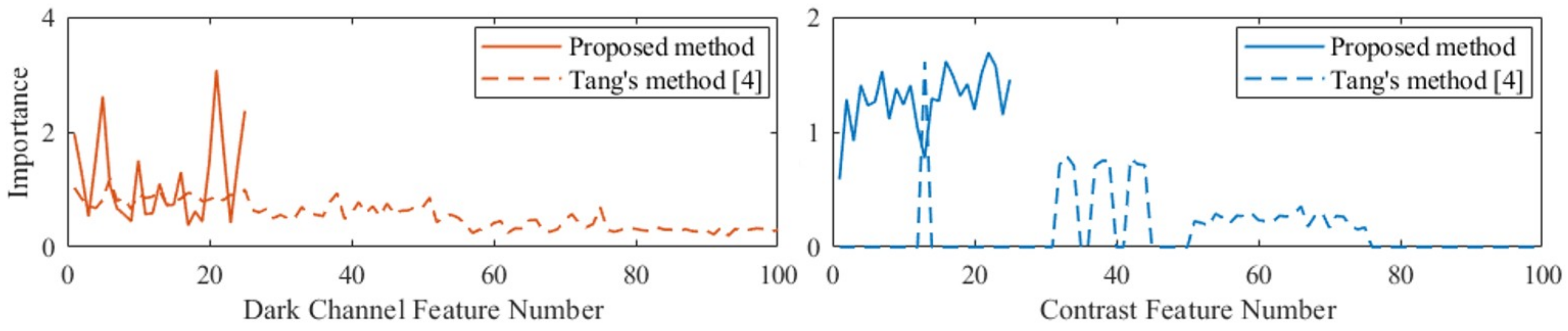
Figure 6.
An image pyramid generated using the haze-free images collected from the internet and estimated transmissions using a single in-scale and multiscaled spaces: (a) an image pyramid [19], (b) an input haze image [16], reproduced with permission from [16], IEEE, 1969 and (c,d) comparative results of transmission estimated using random forest.

Figure 7.
Estimation of the atmospheric light using the proposed and existing methods. The first and second rows respectively show the input haze image and the estimated atmospheric light [20], reproduced with permission from [20], IEEE, 2016. The third row shows the R, G, and B pixel values of estimated atmospheric light: (a) ground-truth, (b) He’s method [1], (c) Sulami’s method [11], (d) Berman’s method [15], reproduced with permission from [15], IEEE, 2017 and (e) the proposed method.
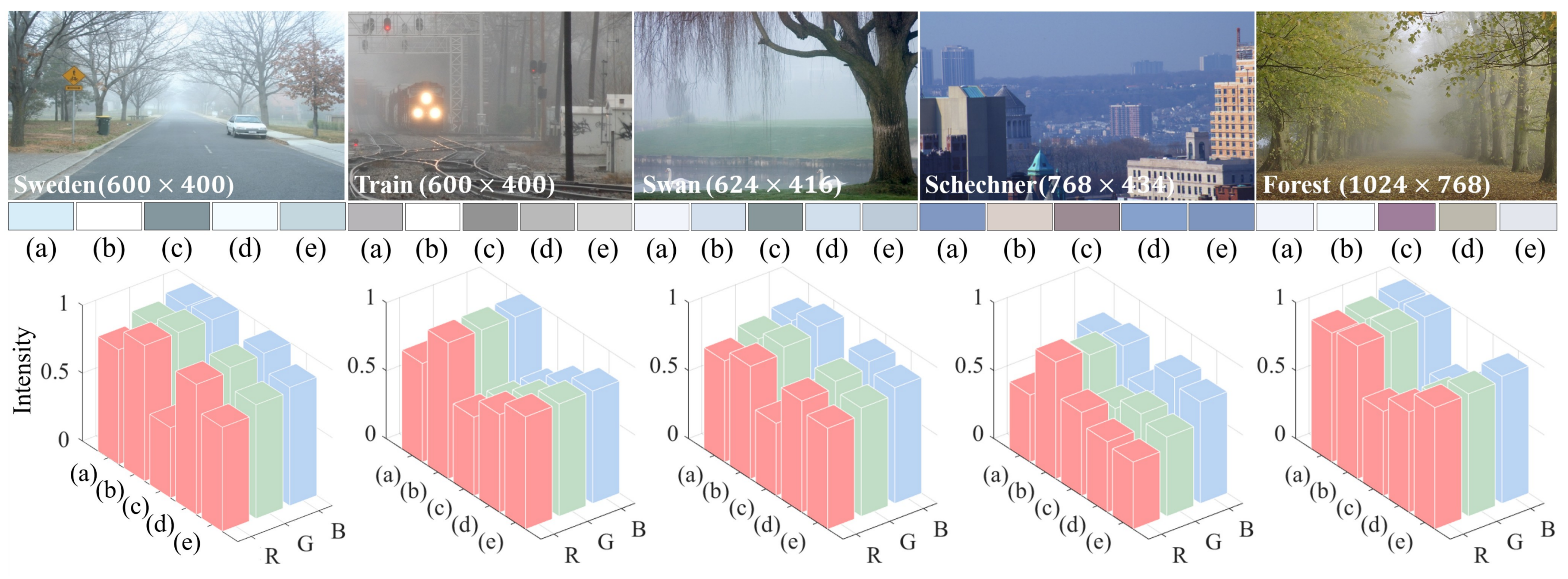
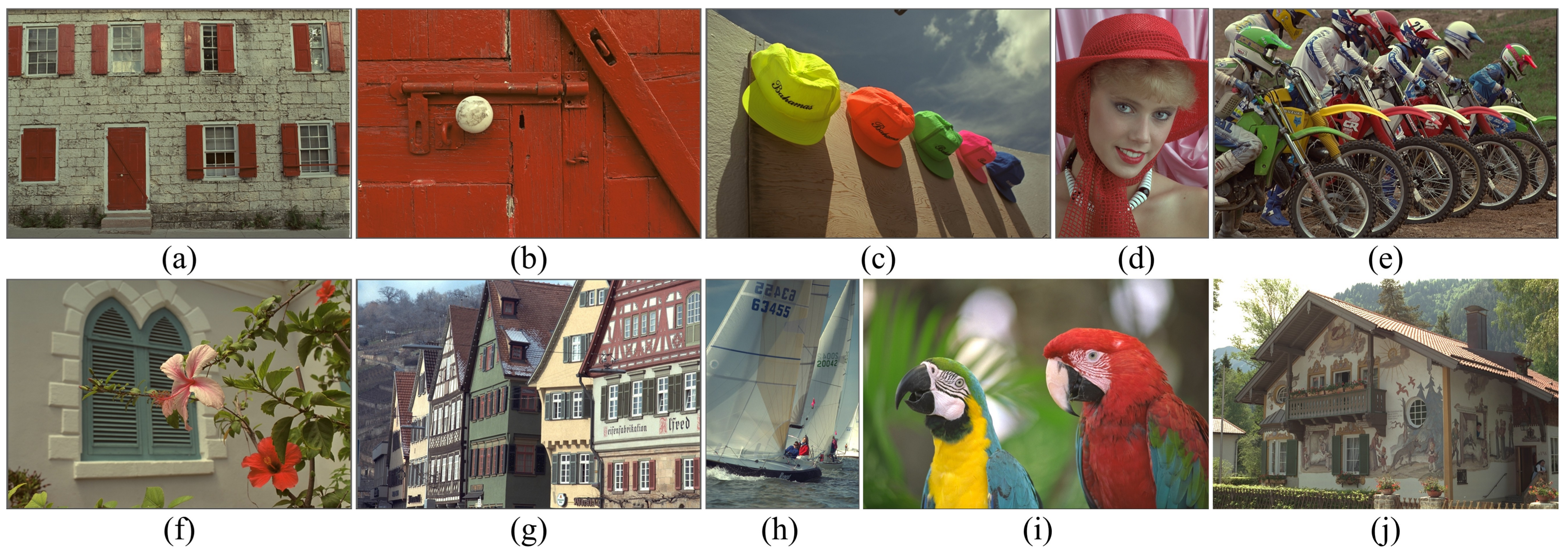
Figure 8.
The test images used for the objective assessment of haze removal [1,4,5,16]: (a–j) are the real haze images to evaluate the performance of haze removal. Reproduced with permission from [1], IEEE, 2011, reproduced with permission from [4], IEEE, 2014, reproduced with permission from [5], IEEE, 2016, reproduced with permission from [16], IEEE, 1969.

Figure 9.
Experimental results of haze removal using the proposed and existing methods: (a) an input haze image [1], reproduced with permission from [1], IEEE, 2011, (b) He’s method [1], (c) Meng’s method [9], reproduced with permission from [9], IEEE, 2013, (d) Berman’s method [8], reproduced with permission from [8], IEEE, 2016, (e) Zhu’s method [2], (f) Ren’s method [6], and (g) the proposed method.

Figure 10.
Experimental results of haze removal using the proposed and existing methods: (a) an input haze image [4], reproduced with permission from [4], IEEE, 2014, (b) He’s method [1], (c) Meng’s method [9], (d) Berman’s method [8], (e) Zhu’s method [2], (f) Ren’s method [6], and (g) the proposed method.
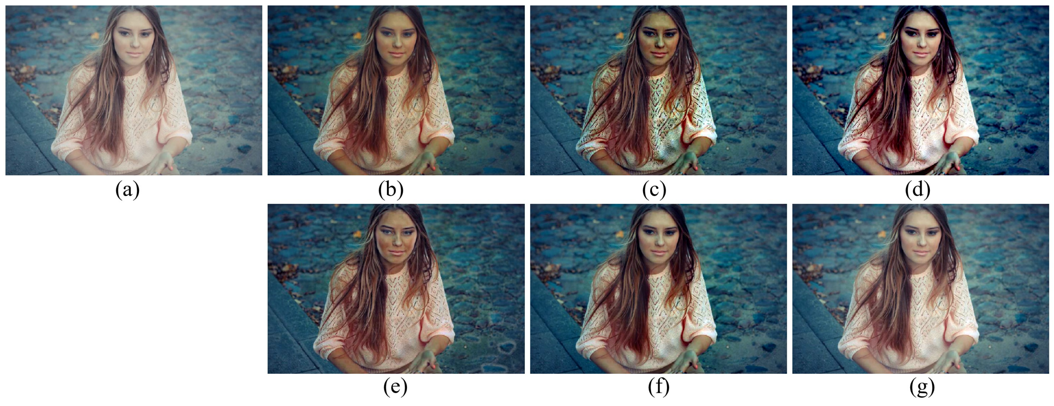
Figure 11.
Experimental results of haze removal using the proposed and existing methods: (a) an input haze image [16], reproduced with permission from [16], IEEE, 1969, (b) He’s method [1], (c) Meng’s method [9], (d) Berman’s method [8], (e) Zhu’s method [2], (f) Ren’s method [6], and (g) the proposed method.

Figure 12.
The test images used for the objective assessments of the performance of transmission estimation [23]: (a)-(e) are the real outdoor haze-free images of size 3873 × 2516. The haze image can be synthesized using corresponding depth map of the haze-free image.
Figure 12.
The test images used for the objective assessments of the performance of transmission estimation [23]: (a)-(e) are the real outdoor haze-free images of size 3873 × 2516. The haze image can be synthesized using corresponding depth map of the haze-free image.

Figure 13.
A set of test images used in the objective assessments of low-light image enhancement [29]: (a–j) are the test images of size 768 × 512 and the low-light image is synthesized by adjusting the non-linear gamma correction.
Figure 13.
A set of test images used in the objective assessments of low-light image enhancement [29]: (a–j) are the test images of size 768 × 512 and the low-light image is synthesized by adjusting the non-linear gamma correction.

Figure 14.
Resulting enhanced images using existing and proposed methods taking synthesized low-light images as the input: (a) ideal image [29], (b) synthesized low-light image, (c) histogram equalization (HE) [26], (d) Huang’s method [27], (e) Jiang’s method [25], and (f) the proposed method.

Figure 15.
Resulting enhanced images of the existing and proposed methods using real low-light images: (a) input image, (b) HE [26], (c) Huang’s method [27], (d) Jiang’s method [25], and (e) the proposed method.

Table 1.
Objective assessments of atmospheric light estimation using the -error and processing time (seconds) [20].
Table 1.
Objective assessments of atmospheric light estimation using the -error and processing time (seconds) [20].
| [1] | [11] | [15] | Proposed | ||||||
|---|---|---|---|---|---|---|---|---|---|
| Error | Time | Error | Time | Error | Time | Error | Time | Time (Parallel) | |
| Sweden | 0.24 | 0.85 | 1.03 | 8.41 | 0.19 | 4.40 | 0.28 | 0.18 | 0.15 |
| Train | 0.82 | 0.67 | 0.45 | 5.43 | 0.03 | 2.25 | 0.30 | 0.34 | 0.29 |
| Swan | 0.23 | 1.72 | 0.68 | 8.36 | 0.21 | 5.10 | 0.02 | 0.22 | 0.21 |
| Schechner | 0.65 | 0.96 | 0.32 | 11.44 | 0.14 | 4.26 | 0.01 | 2.61 | 1.56 |
| Forest | 0.07 | 1.63 | 1.17 | 14.16 | 0.74 | 5.49 | 0.16 | 1.50 | 0.93 |
| Avg. | 0.40 | 1.17 | 0.73 | 9.56 | 0.26 | 4.30 | 0.15 | 0.97 | 0.63 |
Table 2.
Comparison of objective assessments using Hautiere’s method [21].
Table 2.
Comparison of objective assessments using Hautiere’s method [21].
| [1] | [9] | [8] | [2] | [6] | Proposed | |||||||
|---|---|---|---|---|---|---|---|---|---|---|---|---|
| Figure 8a | 0.0000 | 1.0870 | 0.1848 | 1.5752 | 1.8338 | 1.7643 | 0.0011 | 1.4817 | 0.0335 | 1.2680 | 0.0095 | 1.1960 |
| Figure 8b | 0.1664 | 1.6934 | 1.1730 | 2.1021 | 0.2565 | 2.4137 | 0.1468 | 1.7906 | 0.1694 | 1.5785 | 0.2161 | 1.4357 |
| Figure 8c | 0.0451 | 1.3218 | 0.2335 | 2.1207 | 6.8876 | 2.3389 | 0.4164 | 1.5604 | 0.7551 | 1.2884 | 0.3001 | 1.2475 |
| Figure 8d | 0.0000 | 1.1548 | 0.0000 | 1.5989 | 0.1561 | 2.1856 | 0.0000 | 1.3821 | 0.0000 | 1.3001 | 0.0000 | 1.2380 |
| Figure 8e | 0.0168 | 1.6015 | 0.1468 | 2.1761 | 0.2651 | 2.1589 | 0.0485 | 1.7905 | 0.1226 | 1.7027 | 0.1152 | 1.4676 |
| Figure 8f | 0.1256 | 2.2194 | 0.0487 | 2.6322 | 0.0563 | 2.3590 | 0.8070 | 1.9389 | 0.0019 | 1.8372 | 0.4088 | 1.6709 |
| Figure 8g | 0.0285 | 1.0251 | 0.5099 | 1.3173 | 2.0646 | 1.9343 | 0.0801 | 1.2948 | 0.5049 | 1.1967 | 0.2038 | 1.1557 |
| Figure 8h | 0.0003 | 2.6491 | 0.0366 | 3.6266 | 0.1915 | 5.0999 | 0.0000 | 1.7928 | 0.0000 | 1.7705 | 0.0000 | 1.5342 |
| Figure 8i | 0.0000 | 1.2353 | 0.0293 | 2.3817 | 0.3793 | 2.0831 | 0.1233 | 1.3019 | 0.1233 | 1.3019 | 0.0459 | 1.2112 |
| Figure 8j | 0.3083 | 1.1934 | 0.2971 | 1.5665 | 4.7788 | 2.8473 | 54.6675 | 1.6899 | 0.2363 | 1.1427 | 0.2992 | 1.3260 |
| Avg. | 0.0691 | 1.5181 | 0.1660 | 2.1097 | 1.6870 | 2.5185 | 0.7291 | 1.6112 | 0.1947 | 1.4387 | 0.1599 | 1.3469 |
Table 3.
Comparison of the objective assessments of the transmission estimation using random forest.
Table 3.
Comparison of the objective assessments of the transmission estimation using random forest.
| # of Trees | [4] | Proposed | |||
|---|---|---|---|---|---|
| 200 | 200 | 100 | 50 | ||
| Figure 12a | MSE | 0.0600 | 0.0313 | 0.0316 | 0.0324 |
| Figure 12b | MSE | 0.0500 | 0.0428 | 0.0428 | 0.0430 |
| Figure 12c | MSE | 0.0780 | 0.0314 | 0.0316 | 0.0320 |
| Figure 12d | MSE | 0.0693 | 0.0245 | 0.0241 | 0.0252 |
| Figure 12e | MSE | 0.0612 | 0.0384 | 0.0390 | 0.0390 |
Table 4.
The objective assessments of the low-light image enhancement using the peak signal-to-noise ratio (PSNR) and the structural similarity index measure (SSIM) [28].
Table 4.
The objective assessments of the low-light image enhancement using the peak signal-to-noise ratio (PSNR) and the structural similarity index measure (SSIM) [28].
| [26] | [27] | [25] | Proposed | |||||
|---|---|---|---|---|---|---|---|---|
| PSNR | SSIM | PSNR | SSIM | PSNR | SSIM | PSNR | SSIM | |
| Figure 13a | 14.9340 | 0.6473 | 15.2250 | 0.6990 | 13.7155 | 0.7044 | 17.9683 | 0.8122 |
| Figure 13b | 8.9670 | 0.1310 | 12.7210 | 0.5678 | 15.0965 | 0.8063 | 18.1877 | 0.8205 |
| Figure 13c | 14.2907 | 0.4049 | 15.4260 | 0.5586 | 12.9453 | 0.6143 | 18.1130 | 0.5971 |
| Figure 13d | 13.7084 | 0.2131 | 15.7105 | 0.5963 | 14.2142 | 0.6855 | 16.7344 | 0.6968 |
| Figure 13e | 12.8507 | 0.6044 | 15.6484 | 0.6960 | 14.0895 | 0.6400 | 17.5864 | 0.6429 |
| Figure 13f | 14.4912 | 0.3775 | 14.8379 | 0.5650 | 12.6677 | 0.6375 | 19.3865 | 0.7534 |
| Figure 13g | 20.9754 | 0.8128 | 19.0706 | 0.7980 | 14.4191 | 0.7019 | 16.8107 | 0.7687 |
| Figure 13h | 15.6074 | 0.5902 | 15.8949 | 0.6559 | 12.0559 | 0.6022 | 14.5077 | 0.6213 |
| Figure 13i | 15.0136 | 0.3879 | 17.0851 | 0.5924 | 13.9160 | 0.6787 | 17.8701 | 0.7628 |
| Figure 13j | 15.5462 | 0.5564 | 16.7592 | 0.6522 | 12.7164 | 0.5974 | 18.2142 | 0.7238 |
| Avg. | 14.6384 | 0.4725 | 15.8379 | 0.6381 | 13.8536 | 0.6668 | 17.5379 | 0.7200 |
Table 5.
The objective quality assessments of the real low-light image enhancement using the autoregressive-based image sharpness metric (ARISM) [30].
Table 5.
The objective quality assessments of the real low-light image enhancement using the autoregressive-based image sharpness metric (ARISM) [30].
| Input | [26] | [27] | [25] | Proposed | |
|---|---|---|---|---|---|
| ARISM | ARISM | ARISM | ARISM | ARISM | |
| Road | 3.0858 | 5.0867 | 4.5993 | 4.0872 | 4.8857 |
| Beach | 3.0861 | 4.1843 | 3.4659 | 3.4488 | 4.0736 |
| Café | 3.0882 | 4.5606 | 3.9947 | 4.1014 | 4.2017 |
| Avg. | 3.0867 | 4.6105 | 4.0200 | 3.8791 | 4.3870 |
© 2018 by the authors. Licensee MDPI, Basel, Switzerland. This article is an open access article distributed under the terms and conditions of the Creative Commons Attribution (CC BY) license (http://creativecommons.org/licenses/by/4.0/).
Share and Cite
MDPI and ACS Style
Kim, M.; Yu, S.; Park, S.; Lee, S.; Paik, J. Image Dehazing and Enhancement Using Principal Component Analysis and Modified Haze Features. Appl. Sci. 2018, 8, 1321. https://doi.org/10.3390/app8081321
AMA Style
Kim M, Yu S, Park S, Lee S, Paik J. Image Dehazing and Enhancement Using Principal Component Analysis and Modified Haze Features. Applied Sciences. 2018; 8(8):1321. https://doi.org/10.3390/app8081321
Chicago/Turabian StyleKim, Minseo, Soohwan Yu, Seonhee Park, Sangkeun Lee, and Joonki Paik. 2018. "Image Dehazing and Enhancement Using Principal Component Analysis and Modified Haze Features" Applied Sciences 8, no. 8: 1321. https://doi.org/10.3390/app8081321
Note that from the first issue of 2016, this journal uses article numbers instead of page numbers. See further details here.