Structural Reliability Prediction Using Acoustic Emission-Based Modeling of Fatigue Crack Growth

Center for Risk and Reliability, University of Maryland, College Park, MD 20742, USA
*
Author to whom correspondence should be addressed.
Appl. Sci. 2018, 8(8), 1225; https://doi.org/10.3390/app8081225
Submission received: 29 May 2018
/
Revised: 19 July 2018
/
Accepted: 23 July 2018
/
Published: 25 July 2018
(This article belongs to the Special Issue Structural Health Monitoring of Large Structures Using Acoustic Emission–Case Histories)
Abstract
:In this paper, AE signals collected during fatigue crack-growth of aluminum and titanium alloys (Al7075-T6 and Ti-6Al-4V) were analyzed and compared. Both the aluminum and titanium alloys used in this study are prevalent materials in aerospace structures, which prompted this current investigation. The effect of different loading conditions and loading frequencies on a proposed AE-based crack-growth model were studied. The results suggest that the linear model used to relate AE and crack growth is independent of the loading condition and loading frequency. Also, the model initially developed for the aluminum alloy proves to hold true for the titanium alloy while, as expected, the model parameters are material dependent. The model parameters and their distributions were estimated using a Bayesian regression technique. The proposed model was developed and validated based on post processing and Bayesian analysis of experimental data.
1. Introduction
Acoustic emission (AE) technology has the potential for on-line structural health monitoring; a desired procedure for evaluating material degradation in aircrafts. Acoustic emissions are stress waves that propagate through a material as a result of applied stresses. When a material is subjected to cyclic fatigue loading, AE signals may be generated frequently with cracking within the material. These waves can be detected by piezoelectric sensors when placed on the surface of the material. The characteristics of the AE signal are determined by the mechanism that generated the signal, and the means by which it travels through the material and the sensor that transforms the emission into the signal [1].
The most commonly used AE feature for fatigue is the AE counts, which is defined as the number of times that an AE signal amplitude exceeds a predefined subjective threshold value. Other common characteristics used to describe features of an AE hit include the signal’s peak amplitude, risetime, and duration. The amplitude is defined as the maximum voltage value of the signal often reported in decibels, the risetime is the time between the first count and the count with peak amplitude, and the duration is the time between the first and last AE count. These features are illustrated in Figure 1, which shows a typical waveform from an AE hit with the associated features.
Besides relating features from the AE signals to fatigue crack growth, some researchers supplement the AE signals with other crack growth indicators. For example, surface temperature mapping known as thermography has been used to enhance detection of crack initiation and growth. The driving factor for this development is that in addition to the release and propagation of stress waves that are detectable by AE sensors during fatigue crack growth, small amounts of thermal energy are also dissipated. Recent promising researches [2,3,4,5], built on the previous pioneering works on infrared t1hermography and AE signals, have also quantified fatigue crack growth. This paper, however, uses features of AE signals alone to describe fatigue crack growth behavior.
Mechanical structures typically operate under a wide range of loading scenarios. Previously proposed fatigue life models based on the AE signal properties reported by Talebzadeh and Roberts, [6]; Bianocolini [7]; and later by Rabiei & Modarres [8] have not been validated with respect to different loading conditions. These studies were also focused only on studying aluminum alloys. Different material and loading features, such as frequency and loading ratio, may also affect model predictions and can be verified through specially designed experiments.
Several attempts have been made to relate different AE parameters such as AE count, energy, and amplitude to fatigue crack growth, stress intensity factor range (∆K), maximum stress intensity factor (Kmax) and crack growth rates [9,10,11,12,13]. These studies showed that the relationship between the stress intensity factor range and the number of AE counts can be captured by an equation with a form similar to the Paris-Erdogan equation [14,15,16]. A leading general model that relates the AE count rate to the crack growth rate was proposed by Bianocolini [7], and has the following form:
where, c is the AE count, a represents crack size, N is the load cycle, (da/dN) is the crack growth rate, (dc/dN) is the AE count rate, and α1 and α2 are the model parameters. Rabiei and Modarres [11] used a variation of Equation (1) in the form of the linear regression in Equation (2):
where, the error term, ε, in Equation (2) accounts for the difference between the model prediction and the observed AE count rate. The model described by Equation (2) assumes that a small crack may be difficult to measure, and as the crack becomes larger, the measurement of crack length becomes more accurate [17]. In order to capture any changes in the error distribution, it was assumed that the error follows a normal probability density function with zero mean and a standard deviation, s (Equation (3)).
Based on a single experiment, Rabiei [17] concluded that s was independent of crack growth rate. To capture the dependence of the crack length on s, Rabiei [17] assumed that s follows a two-parameter exponential distribution that changes as a function of AE count rates. However, these assumptions were not supported by the results of this research. The experimental results of this study suggested that s follows a normal distribution and is not a function of AE count rates; s ≈ N(μs,σs).
The significance of the proposed model represented by Equations (2) and (3) is that once the model parameters are estimated using experimental data, this equation can be used to estimate crack growth rates of structures by monitoring AE signals and extracting the AE count rate from the observed signals.
Rabiei’s model [17] was derived based on the results from one experiment with sinusoidal loading conditions of a maximum load of Pmax = 300 lbf (1334 kN), loading ratio of R = 0.1, and loading frequency of f = 10 Hz. The results have not been validated with respect to different loading conditions and were limited to one experiment on Al7075-T6. Therefore, the first step in this research was to study the consistency and variability of the model by performing several standard fatigue experiments using compact tension test specimens of the same aluminum alloy (Al7075-T6) subjected to cyclic loading with varied loading ratios and frequencies. This part of the research addressed model development and validation, with respect to changes in loading frequency and loading ratio, through statistical analysis of the crack growth data. In the second step, the material effect was studied based on three identical crack growth tests with Ti-6Al-4V titanium alloy (known as Ti-6-4). Experimental procedures and methods of analyzing the data were similar to those used for the Al7075-T6 samples.
This paper first discusses the details of the performed fatigue experiments, followed by the description of the data analysis methods, and finally presents results including model development and validation. In the final section, conclusions are summarized and suggestions are made for future work.
2. Experimental Approach
The goal of the experiments performed was to monitor fatigue crack propagation in standardized specimens. The test samples for both Al7075-T6 and Ti-6-4 were supplied in the form of compact tension (CT) specimens, based on ASTM standard E647 [18]. The test specimens were manufactured from 0.125 in (3.175 mm) thick plates. The geometry and dimensions of the specimens are shown in Figure 2.
A servo-hydraulic Material Testing System (MTS) fatigue machine retrofitted with an Instron 8800 controller was used to define and control the loading conditions. An advanced DiSP-4 AE system supplied by the Physical Acoustics Corporation (now MISTRAS Group), was used to record the AE signals. The setup included one 100–900 kHz wideband differential AE sensor (WD) to collect the signal, a 40 dB preamplifier to amplify them, a data acquisition module to perform primary filtration and record the signals, and a software module to visualize the data and to perform feature extraction.
A ruler with smallest divisions of 0.01 in. (0.254 mm) was placed on the specimen so the actual crack length could be measured during post-processing of the images. The AE sensor was attached to the upper left-hand side of the specimen with silicone grease and held in place with a C-clamp (Figure 3). The instrumented CT specimens were mounted on the 5 kip MTS machine which applied sinusoidal loading cycles until a fatigue pre-crack of adequate length and straightness (according to ASTM E647) could be detected. Then, the standard crack growth tests were conducted using the same MTS machine. All the experiments were continued until fracture.
A 40 dB preamplifier amplified the AE signals received from the sensor. A band pass filter was used in the amplifier, and the amplified signals were analyzed using the DiSP-4 system. The AE features that were measured and recorded included AE counts, energy, and the time of the event. A digital close-up camera took time-lapsed high-resolution pictures of the crack growth, and the crack length could be measured based on the ruler attached onto the specimen within the accuracy of 0.01 inch (0.254 mm). As a result, considerable amounts of data were captured and stored for further processing.
Experiments performed on several CT specimens were subjected to cyclic loading with different loading ratios. For each case, the loading ratio was changed, with all other test parameters remaining constant. Table 1 lists the experiments performed for the corresponding load ratios:
For the three Ti-6-4 tests, the loading was increased because Ti-6-4 has a higher yield strength of about 120 ksi (830 MPa) compared to the yield strength of Al7075-T6 of about 67 ksi (460 MPa) [19]. Additionally, the frequency was decreased to 5 Hz in order to better distinguish and process AE events during post-processing [20].
Noise Reduction
AE signals may be generated from a number of possible sources including background noise, micro-crack generation, or plastic deformation. In order to reduce uncertainties and determine the AE signals corresponding to crack growth, applying noise reduction techniques on the captured data was required. Various de-noising techniques have been proposed to filter AE signals due to extraneous events during crack growth [10,21,22].
To filter out noise from AE signals associated with fatigue crack propagation, the recorded AE data was filtered using the acquisition system’s band pass filter (200 kHz–3 MHz). In addition to the band pass filter that restricts the captured signals based on frequency, an amplitude threshold was determined and filtered out low-amplitude background noise. It should be noted that the lack of significant AE activity in the initial stages of fatigue loading makes it more difficult to distinguish background noise from crack-related acoustic events. For each set of materials, a dummy specimen was tested beforehand under the same conditions as the main experiments to determine the background noise. The dummy specimen was simply the first sample from the test specimen batch and had the same geometry and characteristics. The dummy specimen was installed in the testing machine, and the background noise was captured as a cyclic load was applied for a few cycles. Based on this test, the AE detection threshold was set to 45 dB for Al7075-T6 samples to eliminate the background noises. This value was found to be 35 dB for the Ti-6-4 samples.
It has also been observed that AE events occurring during the loading portion of a cycle are related to crack growth [6,17,21]. Therefore, the AE data taken only during the loading portion of each cycle were used for data analysis, while AE events during the unloading portion of the cycle were ignored. In addition, many researchers have assumed that only events occurring close to the maximum or peak load are associated directly with crack growth [12,21,22]. So, the filtered AE events were separated for different percentages of the applied load range, and it was determined that the AE counts occurring within the top 20% of peak load showed the closest correlation with crack propagation rates [23].
3. Analysis of Experimental Data and Results
3.1. Crack Growth Measurement
The lengths of the pictured cracks were measured using an image processing software called ImageJ [24]. Crack measurement with the image processing software was calibrated using the scale ruler attached to the specimen. The accuracy of the ruler was 0.01 in. (0.254 mm); therefore, the scale error was estimated as ±0.005 in. (0.127 mm). One example of the process for measuring the crack length and matching the crack length with the cumulative AE counts is shown in Figure 4. By knowing the crack length and AE cumulative counts at numerous instances during the experiment, values for crack growth rate and AE count rate were estimated.
When the crack lengths were determined, the fatigue crack growth rates were approximated at different cycles using Equation (4):
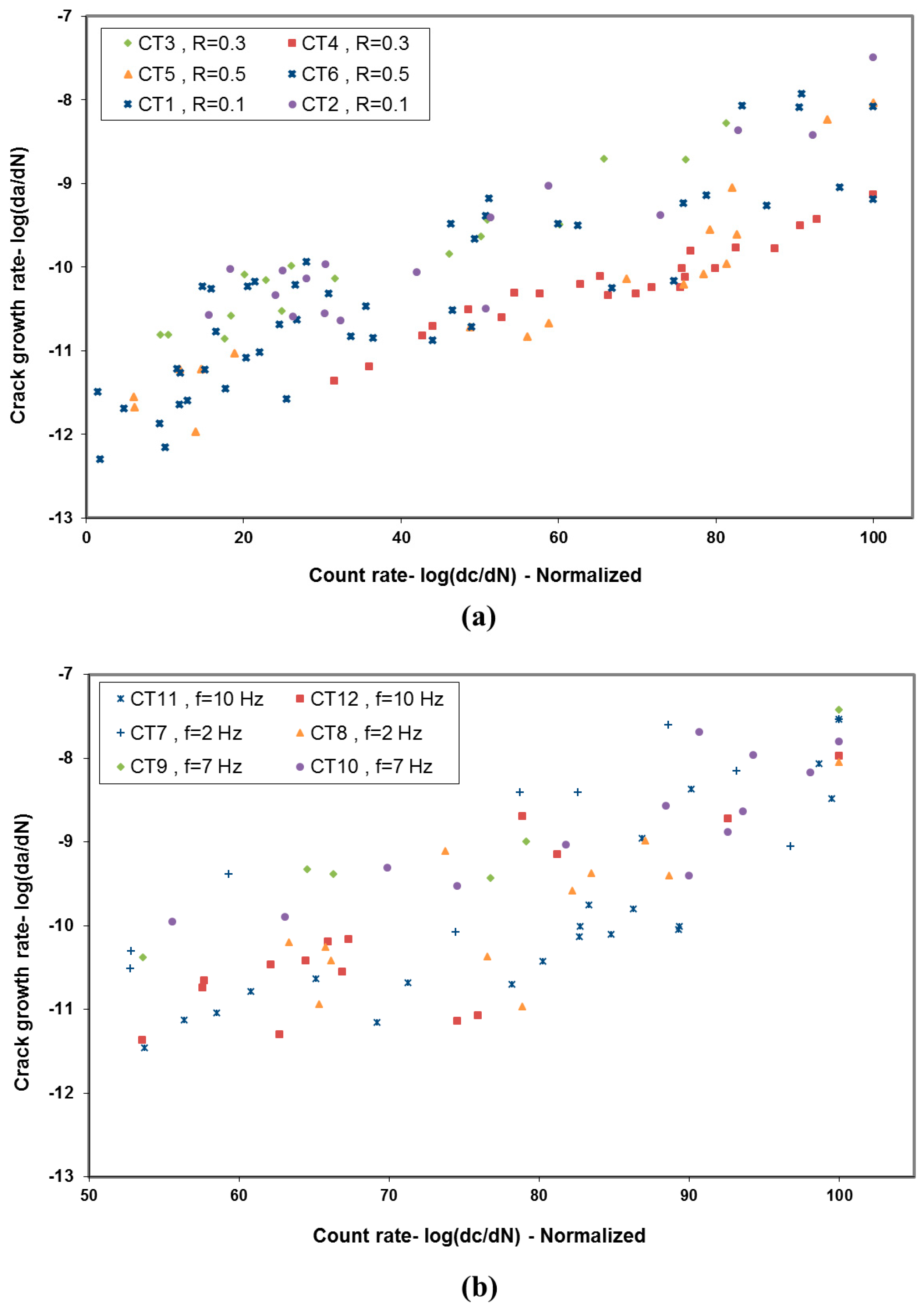
According to the observed data, the correlation between the AE count rates and stable crack growth rates follow the log-linear model of Equation (2). To properly compare the correlations estimated from all observed data obtained from different fatigue loading conditions on a similar scale, the correlation between the logarithm of crack growth rate and the normalized logarithm of dc/dN values was found. That is, the logarithm of every count rate was normalized to the range of the logarithms of minimum and maximum count rates observed in each test. With this normalization, the estimated parameters of Equation (2) were nearly identical for each test regardless of the loading ratio or loading frequency and thus allowed all tests data to be combined to estimate one correlation model, as discussed in Section 3.3. Therefore, every dc/dN data point can be reversely expressed in terms of the corresponding normalized value and the two fixed minimum and maximum log(dc/dN) values. The correlation between normalized log(dc/dN) and log(da/dN) for different experiments at different loading ratios is shown in Figure 5a. Similarly, results for tests at different loading frequencies is shown in Figure 5b.
After the post processing of the AE data, the experimental results were used to determine the point estimate unknown parameters α1 and α2 in Equation (2) using regression analysis. The observed correlation of AE count rates versus crack growth rates and the regression analysis of the experimental data corresponding with different frequencies and different loading ratios showed that estimated parameters of the regression line are in the same range and do not have a considerable difference. It should be noted that the mean value of the regression parameters are calculated using all the experimental data and the estimation of the error term was implemented later in the probabilistic model development section. The point estimates of the linear regression model parameters for the different experiments are listed in Table 2. It should be noted that the fatigue lives (cycles-to-fracture) for Al7075-T6 samples were in the range of 3500 and 12,000 cycles. This range was determined to be 45,000 to 109,000 cycles for the Ti-6-4 samples.
3.2. Test of Homogeneity
To determine if there is any significant statistical difference in the regression lines derived from the different test data, an Analysis of Covariance (ANCOVA) was used [25]. The topic of interest is whether the regression lines have similar slopes. This method allows for testing the null hypothesis that the regression model parameters were derived from samples estimating populations which all had equal slopes.
For this hypothesis analysis, the confidence limit level was selected to be 90% (i.e., Pcritical = 0.05). The F statistic was calculated as 0.82 and the corresponding probability (p-value) was estimated to be 0.618. Since F statistic is less than unity and p-value is greater than Pcritical, the null hypothesis could not be rejected. It was concluded that there is no statistically significant difference between the slopes of regression lines and the test of ANCOVA confirmed that the model is not influenced by the loading ratio and loading frequencies. For more information about ANCOVA, refer to References [26,27].
3.3. Probabilistic Model Development
Since the results show that changes in certain loading conditions do not result in any significant influences on the linear model of AE count rate versus crack growth rate, all the experimental data from different tests could be used to develop the crack length vs. AE count rate model. To do this, the experimental data set for Al7075-T6 was divided into three different sets. One set was used for parameter estimation when defining the model, one set was used for evaluating the error term in the model, and the final data set was used for model validation. The first set was of four experiments that were selected from different loading conditions to arrive at a more generic model in the phase of model development. Those experiments were CT1, CT3, CT5 and CT7 from Table 1. The second set of data used to estimate the uncertainties and capture the error term in the model were CT2, CT4, CT6, CT10 and CT12 from Table 1. The last step was to validate the developed model. The experiments used for validation were CT9 and CT11 from Table 1. The procedure and results of model development and validation are reported in the remainder of this section.
3.3.1. Bayesian Data Analysis
A Bayesian regression approach was implemented to estimate the model parameters and error. This technique is used to estimate and update the posterior distribution of the unknown model parameters [28]. In the Bayesian inference, a prior probability distribution function (pdf) of the model parameters is combined with observed data (evidence) in the form of a likelihood function of an unknown parameter (θ). The result is an updated state of knowledge in the form of the posterior joint distribution of the model parameters, f(θ|x). The posterior pdf of the model parameter can be assessed as described according to the Bayes’ Theorem [29] as:
where, f(θ|x) is the posterior pdf of the vector of parameters (θ) given the observed data (x); f(x) is the marginal pdf of the random variable x; f(θ) is the prior pdf of the model parameters; and f(x|θ) is the likelihood of the model and contains the available information provided by the observed data:
The results of the analyzed experimental data were used to develop a probabilistic linear model for the estimation of the crack growth rate as the dependent variable, and using the AE count rate as the independent variable. So, based on the observed correlation, the unknown parameters of the linear model described in Equation (2) are updated. An error term was added later to assess the model error.
After the first steps of analyzing the experimental data (crack growth measurement, AE data filtration, and AE count rate calculations) were completed, the results were used to estimate the marginal and joint distribution of the unknown parameters in Equations (2) and (3) using the Bayesian regression using Equations (5) and (6). The software package WinBUGS [28] was used to perform the Bayesian inference. In this Bayesian inference, the likelihood function in Equation (6) for the observed independent crack data points (xi, yi) can be expressed as a normal distribution:
where p(.) is the likelihood of all data in form of xi = log(dc/dN)i, yi = log(da/dN)i, and D is the data set of all pairs (xi, yi) for i = 1 to n of the tests.
3.3.2. Error and Uncertainty
Uncertainties associated with the model have various sources which may be grouped as follows:
- (a)
- Aleatory uncertainty: Also known as inherent uncertainty, aleatory uncertainty is a natural randomness of a quantity such as uncertainty in the material features. Generally, there are different factors during manufacturing of a material that cause random variation of the material properties from experiment to experiment [30]. To minimize aleatory uncertainty, test data of specimens from the same material lot (test samples coming from the same sheet of Al7075-T6 or Ti-6-4) were used. It should be noted that this physical variation is inherent to experiments and cannot be eliminated.
- (b)
- Epistemic uncertainties: This uncertainty is the result of limited information or incomplete information due to finite experimental data or a limited number of observed data points. The addition of experiments corresponding with each loading condition in the parameter estimation process can help reduce epistemic uncertainty bounds for the estimated model parameters. Two types of epistemic uncertainty are discussed below:
1. Measurement error: This is the error caused by imperfect measuring equipment and/or human observation errors. There are some inherent variations resulting from the method of observation. The image processing method used for measuring the specimen’s crack length based on the high-resolution photography with the close-up lens carried some measurement errors due to difficulties in finding the crack tip in images.
Some methods were applied to reduce the crack length measurement error. If the measurement value is known to be constant from one measurement to another and if the measurement can be made several times, information about the uncertainty of the measuring method can be obtained. In this case, this type of uncertainty can be reduced through averaging. It was attempted in this research to reduce the measurement uncertainty using the measurement data produced by two different individual testers on each data point. Since these measurements are mutually independent the mean value of the measured crack length was used for each data point.
2. Modeling error: Besides the error of crack length measurement, filtration method and insufficient data, there is an important model uncertainty that must be captured. This model uncertainty is related to the formulation of the proposed probabilistic model. There might be some other sources of uncertainty that can be considered such as the uncertainty resulting from the de-noising technique. For example, the noise reduction method may filter out some crack growth related signals and contribute to the model uncertainty. Improvement can be made by exploring alternate methods of classification of AE-related data and filtration techniques.
In Section 3.3.2.1, the AE model error is estimated, which expresses the sum of aleatory and epistemic uncertainties described above. Later in Section 3.4, the model is validated and the uncertainties are estimated.
3.3.2.1. Model Error Estimation
After establishing a linear relationship between the explanatory variable, dc/dN, and the response variable, da/dN, the relationship can be used to make predictions of the next value of crack growth rate given the next value of AE count rate. Predicting future observations for certain dc/dN values is one of the main goals of this linear regression modeling. Better prediction can be made considering the uncertainties and errors in the model. True values for model parameters are unknown and using estimated values in the prediction adds to the uncertainty that should be captured by the error term. The error term showed by ε in Equation (2) includes all the uncertainties discussed in the previous section and follows a normal distribution with the mean of zero and standard deviation that needs to be captured (s). The results of this study showed that parameter s of the error term can be described by another normal distribution: s ~ N(μs, σs).
The point estimates of the model parameters, α1 and α2, and the model error, ε, described by Equations (2) and (3) were computed for Al7075-T6 and Ti-6-4 experiments separately. As discussed, the error term is considered to follow a normal distribution with the mean of zero and a standard deviation of s which accounts for the model uncertainties after the data were normalized. The model parameters and error term distributions were determined through Bayesian analysis for each set of experiments. The software WinBUGS was used to capture the error term distribution in the model in which uninformative, or uniform, prior distributions were chosen for all variables. The posterior distributions of the error term and the corresponding standard deviations were determined and are listed in Table 3.
The error estimation for Al7075-T6 tests was performed by comparing experimental measurements with estimated model predictions obtained through Bayesian analysis (using parameter estimation for Al7075-T6 in Table 3). Subsequently, it was found that for Al7075-T6, the parameter s of the error term follows a normal distribution as well and was estimated as s ~ N(0.86, 0.057), where ε ~ N(0, s). The results are shown in Figure 6.
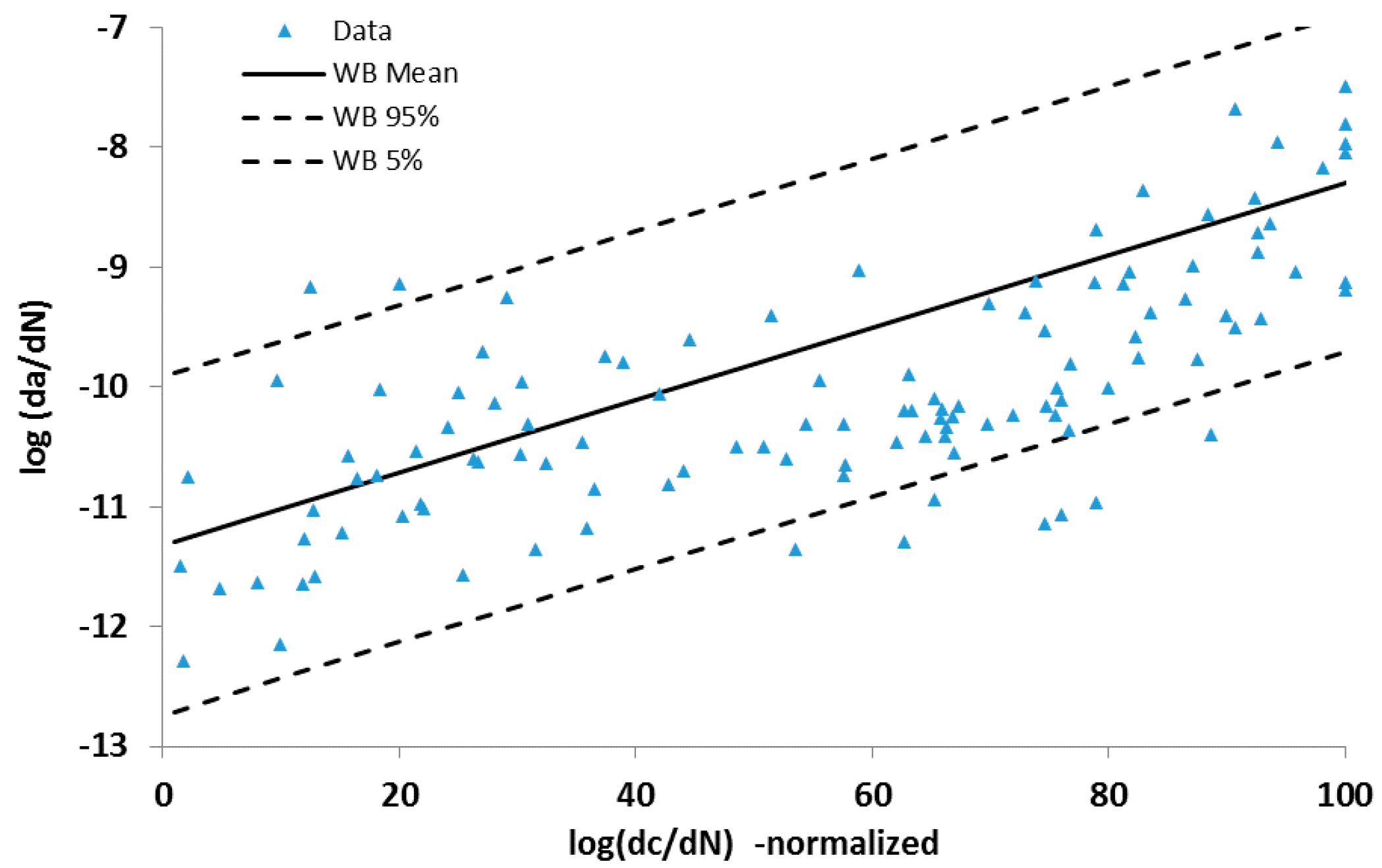
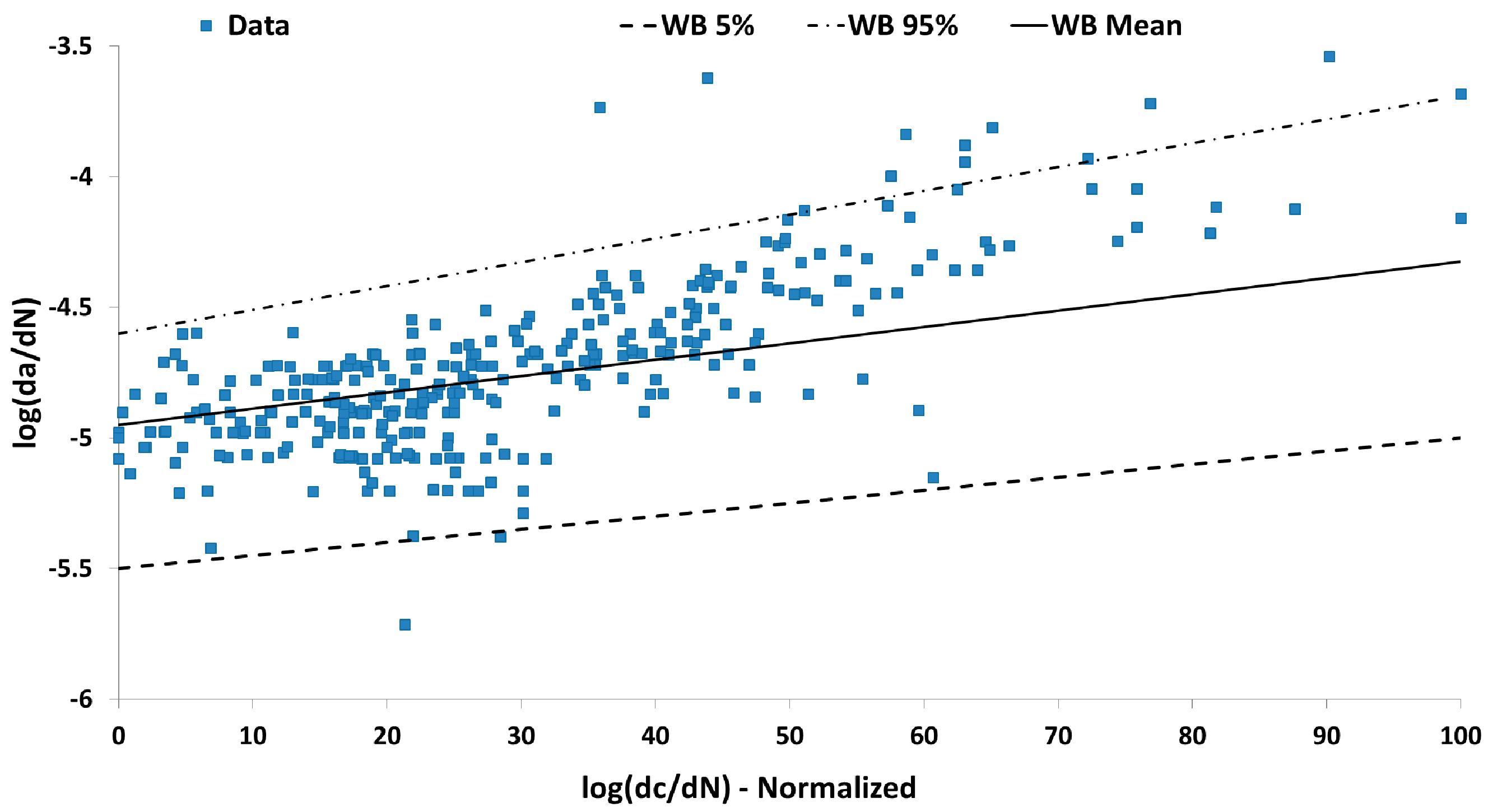
The result of the posterior predictive distribution for da/dN as a function of dc/dN for Al7075-T6 is plotted in Figure 7. The posterior distribution is shown by its median and the 95% confidence level (2.5% and 97.5% prediction bounds). The data used to fit the model is also plotted in Figure 7.
Each of the three Ti-6-4 experiments demonstrated a good correlation between AE count rate and crack growth rate. These results suggest that the proposed linear model based on Al7075-T6 holds for the Ti-6-4 as well. The regression between log(da/dN) and log(dc/dN) for the experiments and confidence interval are depicted in Figure 8. As expected, the model parameters are considerably different between Al7075-T6 and Ti-6-4 testing, but the form of the model remains unchanged. To provide a visual comparison, the linear regressions between crack growth rate and AE count rate and the raw data for Al7075-T6 and Ti-6-4 are displayed in Figure 9.
This finding suggests that since almost all procedures were maintained between the two sets of experiments, the model parameters must be updated to account for material variation from material to material, as expected. In addition, both model parameters are material-dependent since both vary significantly between the material testing.
Some inferences about AE phenomena in different materials can be made by comparing the regression parameters listed in Table 3. The slope parameter, α1, for the Ti-6-4 is smaller than the reported α1 value for Al7075-T6. This relationship suggests that as the AE count rate increases, less increase is observed in the crack growth rate in the Ti-6-4 as compared to Al7075-T6. The intercept parameter, α2, for the Ti-6-4 is larger than Al7075-T6. Physically, this means that a crack will generally grow at a faster rate in the Ti-6-4 than Al7075-T6 for the same relative AE count rate. In other words, as a crack propagates, higher crack growth rates are detected for the Ti-6-4 than Al7075-T6. The tradeoff when detecting crack growth through means of observing AE count rate is a crack will grow more quickly but at a relatively consistent rate for Ti-6-4, compared to a slower but relatively variable crack growth rate in Al7075-T6. Finally, it should be noted that the differences in the crack growth models are simplified into two dimensions, the two model parameters, α1 and α2. If the relationships between log(da/dN) and log(dc/dN) for Ti-6-4 were not linear, at least one other material-dependent dimension would need to be considered.
3.4. Model Validation
In order to validate the developed AE model, model predictions of crack growth rate were compared against the validation experimental data set. For a given value of AE count rate, a prediction of crack growth rate was estimated based on the developed AE-based model. Available information captured from Al7075-T6 experimental data was used as the input to the Bayesian estimation procedure, as the model was developed based on Al7075-T6 data. The Bayesian estimation approach updated the model prediction with the experimental results. With this Bayesian estimation inference, uncertainties in the experimental values were propagated in the model and resulted in model prediction uncertainty assessment. The prediction results were then compared against the true crack growth rates obtained by validation experiments.
In the proposed model validation methodology [31], both model prediction and experimental results are considered to be estimations and representations of the true values, given some error as it is shown in Equations (8) and (9):
and
where Xi is the true value, Xe,i and Xm,i indicate the experimental results and model prediction, respectively. Fe is the multiplicative error of the experiment with respect to true value, and Fm is the multiplicative error of the model prediction with respect to true value. A multiplicative error of the experiment with respect to the model prediction is defined by Equation (10):
Since both Fm,i and Fe,i distributions are lognormal, the distribution of Ft,i would also be lognormal with mean and standard deviation of (bm − be) and , respectively. In this approach, the likelihood used is shown in Equation (11):
Using the validation sets of data, the validation approach was implemented and the results are discussed in this section. For more information about the validation method, refer to the paper by Ontiveros [31]. For simplicity, the distributions of model predictions were reduced to a mean value and compared one-to-one with the experimental results. The mean and standard deviation of Fe, which are be and se, were determined from the unbiased experimental error of ±1%. The values determined were −0.00002 for be and 0.002 for se. The summary statistics for the marginal posterior pdf of parameters bm and sm as well as the distribution of Fm are presented in Table 4.
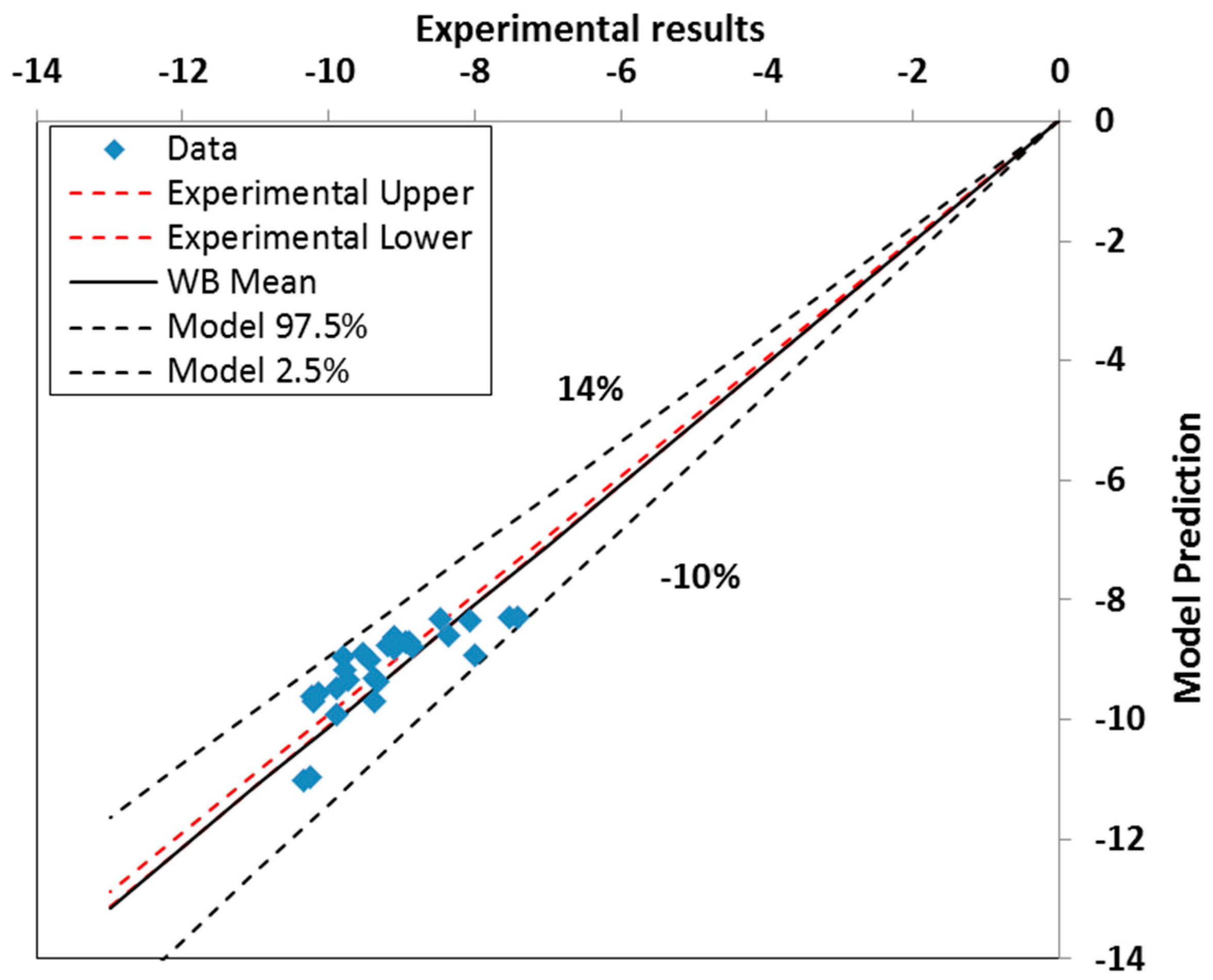
The model uncertainty bounds for the crack length estimation can be determined from the 2.5 and 97.5 percentile of the multiplicative error of Fm. The resulting upper bound on reality was calculated as 14%, while the lower bound is −10%. These results are presented graphically in Figure 10. It can be noticed that the mean values of the model prediction are standing on the upper bounds of the experimental error, and the value of Fm for the model prediction is greater than 1. The value of Fm around 1.01 suggests a very small bias in the AE model to under predict the true crack growth rate. Therefore, the estimation of the true crack growth rate given by the model prediction is expected to be slightly higher. The results show that to correct the model, the predictions must be increased by a factor of 1.01.
Using the experimental data points for log(da/dN) and assuming an experimental error of ±1%, the 45-degree solid line shows the difference between the model prediction and the “true” log(da/dN) (with the 45-degree line showing the perfect match). However, because of the experimental data scatter and a slight bias expressed by Fm (showing systematic model error) between the true log(da/dN) and regression models of Figure 9, the true log(da/dN), with a 95% confidence level, will be somewhere as high as 14% above the model prediction and as low as 10% below this prediction.
As expected, the validation results showed good agreement between model predictions and experimental observations. The validated AE model can be used in real time monitoring of large cracks that subsequently improves the structural health management.
4. Conclusions
This research focused on the AE model for large crack growth assessment. In order to establish the AE signal feature versus the fatigue crack growth model and study the consistency and accuracy of the model, several standard fatigue experiments were performed. A set of tests were performed using standard Al7075-T6 test specimens subjected to cyclic loading with different amplitude and frequencies. A previously proposed relationship between the crack growth rate and AE signal features generated during crack growth was modified and validated. The AE-based crack growth model was found to be independent of the loading condition and loading frequency. These findings validate the previous work by Rabiei [17] as the proposed model is independent of the loading ratio and frequency.
Based on three identical tests with Ti-6-4, it was concluded that while the model parameters are material-dependent, the linear model form depicting the relationship between the crack growth rate and AE count rate remains valid when the material is changed.
The obtained experimental data was uncertain in nature due to considerable uncertainties in the optical crack detection method and measurement errors associated with the utilized crack sizing technique. The procedure of probabilistic model development and validation were discussed, and uncertainties of the model were investigated. To deal with uncertainties, a Bayesian approach was used to consider systematic and random errors in the model by capturing the effect of uncertainties. This approach provided a framework for updating the distribution of the model parameters.
Development of the proposed AE monitoring technique reported in this paper facilitates for the prognostics and life predictions of the structure. The developed methodology can be utilized for continuous in-service monitoring of structures and has proven to be promising for use in life predictions and assessment for structures subject to fatigue loading. Ultimately, these predictions can be used to define the appropriate inspection policies and maintenance schedules.
To update the model for any material variation, quantitative material properties that correlate to the AE count rate and crack growth rate could be identified. This process would be extensive due to the numerous material properties that affect a material’s failure mechanisms including fracture toughness, modulus of elasticity, and yield strength. Once properties are identified, numerous types of materials could be tested to validate and update the model to account for material variations. In addition, the model is based on tests using the same specimen geometry of a specific plate thickness. Since crack growth behavior can also be dependent on the thickness of the material, the AE response and subsequently the model would be dependent on material thickness and specimen geometry. Future research may also focus on experimental studies to account for the effects of material thickness.
Author Contributions
A.K. developed and performed the Al7075-T6 acoustic emission and fatigue crack growth experiments while C.S. performed the Ti-6-4 experiments. A.K. and C.S. each performed the initial data analysis steps including crack growth measurements, de-noising, and AE count rate calculations for each of their respective experiments. A.K. performed the Bayesian analysis and model parameter development for all tests. A.K. wrote the majority of the paper, while C.S. contributed to several sections and assisted in editing. Finally, M.M. was the academic research advisor in this work and provided guidance throughout the research and edited the paper.
Conflicts of Interest
The authors declare no conflict of interest.
References
- Beattie, A.G. Acoustic emission, principles and instrumentation. J. Acoust. Emiss. 1983, 2, 95–128. [Google Scholar]
- Vanniamparambil, P.A.; Guclu, U.; Kontsos, A. Identification of crack initiation in aluminum alloys using acoustic emission. Exp. Mech. 2015, 55, 837–850. [Google Scholar] [CrossRef]
- Barile, C.; Casavola, C.; Pappalettera, G.; Pappalettere, C. Analysis of crack propagation in stainless steel by comparing acoustic emissions and infrared thermography data. Eng. Fail. Anal. 2016, 69, 35–42. [Google Scholar] [CrossRef]
- Kordatos, E.Z.; Aggelis, D.G.; Matikas, T.E. Monitoring mechanical damage in structural materials using complimentary NDE techniques based on thermography and acoustic emission. Compos. Part B Eng. 2012, 43, 2676–2686. [Google Scholar] [CrossRef]
- Barile, C.; Casavola, C.; Pappalettera, G.; Pappalettere, C. Acoustic sources from damage propagation in Ti grade 5. Measurement 2016, 91, 73–76. [Google Scholar] [CrossRef]
- Roberts, T.M.; Talebzadeh, M. Acoustic emission monitoring of fatigue crack propagation. J. Constr. Steel Res. 2003, 59, 695–712. [Google Scholar] [CrossRef]
- Biancolini, M.E.; Brutti, C.; Paparo, G.; Zanini, A. Fatigue cracks nucleation on steel, Acoustic emission and fractal analysis. Int. J. Fatigue 2006, 28, 1820–1825. [Google Scholar] [CrossRef]
- Rabiei, M.; Modarres, M.; Hoffman, P. Quantitative Methods for Structural Health Management using in-situ AE Monitoring. In Proceedings of the Annual Conference of the Prognostics and Health Management (PHM) Society, Montreal, QC, Canada, 25–29 September 2011. [Google Scholar]
- Bassim, M.N.; Hamel, F.; Bailon, J.P. Acoustic emission mechanism during high-cycle fatigue. Eng. Fract. Mech. 1981, 14, 853–860. [Google Scholar]
- Roberts, T.M.; Talebzadeh, M. Fatigue life prediction based on crack propagation and acoustic emission count rates. J. Constr. Steel Res. 2003, 59, 679–694. [Google Scholar] [CrossRef]
- Rabiei, M.; Modarres, M. Quantitative methods for structural health management using in situ acoustic emission monitoring. Int. J. Fatigue 2013, 49, 81–89. [Google Scholar] [CrossRef]
- Han, Z.; Luo, H.; Cao, J.; Wang, H. Acoustic emission during fatigue crack propagation in a micro-alloyed steel welds. Mater. Sci. Eng. A 2011, 528, 7751–7756. [Google Scholar] [CrossRef]
- Strantza, M.; Hemelrijck, D.; Guillaume, P.; Aggelis, D.G. Acoustic emission monitoring of crack propagation in additively manufactured and conventional titanium components. Mech. Res. Commun. 2017, 84, 8–13. [Google Scholar] [CrossRef]
- Gong, Z.; Nyborg, E.O.; Oommen, G. Acoustic emission monitoring of steel railroad bridges. Mater. Eval. 1992, 50, 883–887. [Google Scholar] [CrossRef]
- Bassim, M.N.; St. Lawrence, S.; Liu, C.D. Detection of the onset of fatigue crack growth in rail steels using acoustic emission. Eng. Fract. Mech. 1994, 47, 207–214. [Google Scholar] [CrossRef]
- Paris, P.; Erdogan, F. A critical analysis of crack propagation laws. J. Basic Eng. 1963, 85, 528–533. [Google Scholar] [CrossRef]
- Rabiei, M. A Bayesian Framework for Structural Health Management Using Acoustic Emission Monitoring and Periodic Inspections. Ph.D. Dissertation, Department of Mechanical Engineering, University of Maryland, College Park, MD, USA, 2011. Available online: https://search.proquest.com/docview/880410901?pq-origsite=gscholar (accessed on 15 July 2013).
- ASTM. Constant Load Amplitude Fatigue Crack Growth Rate above 10−8 m/cycle; American Society for Testing and Materials: Washington, DC, USA, 2008; pp. 321–339. [Google Scholar]
- Gauthier, M.M. Engineered Materials Handbook—Desk Edition; ASM International: Materials Park, OH, USA, 1995. [Google Scholar]
- Sauerbrunn, C.M.; Modarress, M. Effects of Material Variation on Acoustic Emissions-Based, Large-Crack Growth Model. In Proceedings of the 25th American Society of Nondestructive Testing (ASNT) Research Symposium, New Orleans, LA, USA, 11–14 April 2016. [Google Scholar]
- Morton, T.M.; Harrington, R.M.; Bjeletich, J.G. Acoustic Emission of fatigue crack growth. Eng. Fract. Mech. 1973, 5, 691–697. [Google Scholar] [CrossRef]
- Wang, Z.F.; Li, J.; Ke, W.; Zhu, Z. Characteristics of acoustic emission for A537 structural steel during fatigue crack propagation. Scr. Metall. Mater. 1992, 27, 641–646. [Google Scholar] [CrossRef]
- Keshtgar, A.; Modarres, M. Acoustic emission-based fatigue crack growth prediction. In Proceedings of the 2013 Reliability and Maintainability Symposium (RAMS), Orlando, FL, USA, 28–31 January 2013; pp. 1–5. [Google Scholar]
- Ferreria, T.; Rasband, W. ImageJ User Guide; U.S. National Institutes of Health: Bethesda, MD, USA, 2012.
- Keshtgar, A. Acoustic Emission-Based Structural Health Management and Prognostics Subject to Small Fatigue Cracks. Ph.D. Dissertation, University of Maryland, College Park, MD, USA, 2013. [Google Scholar]
- Miller, G.A.; Chapman, J.P. Misunderstanding analysis of covariance. J. Abnorm. Psychol. 2001, 110, 40–48. [Google Scholar] [CrossRef] [PubMed]
- Smith, F. Interpretation of adjusted treatment means and regression in analysis of covariance. Biometrics 1975, 13, 282–308. [Google Scholar] [CrossRef]
- Ntzoufras, I. Bayesian Modeling Using WinBUGS; John Wiley and Sons: Hoboken, NJ, USA, 2009. [Google Scholar]
- Bolstad, W.M. Introduction to Bayesian Statistics, 2nd ed.; John Wiley and Sons: Hoboken, NJ, USA, 2007. [Google Scholar]
- Ditlevsen, O.; Madsen, H.O. Structural Reliability Methods; John Wiley and Sons: Hoboken, NJ, USA, 2007. [Google Scholar]
- Ontiveros, V. An Integrated Methodology for Assessing Fire Simulation Code Uncertainty. Master’s Thesis, University of Maryland, College Park, MD, USA, 2010. [Google Scholar]
Figure 1.
Characteristics of AE Signal.
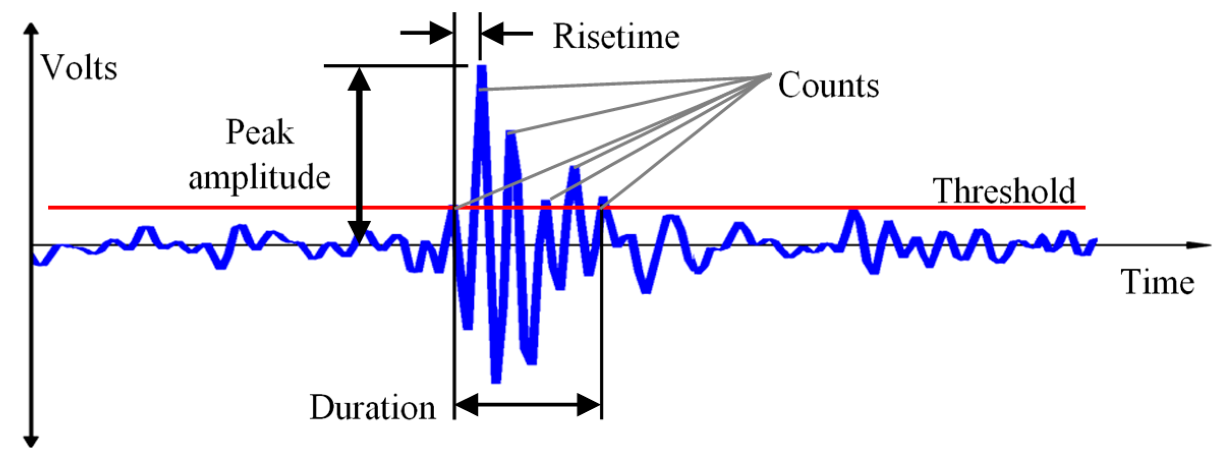
Figure 2.
Technical drawing of the CT specimen (dimensions in inches).
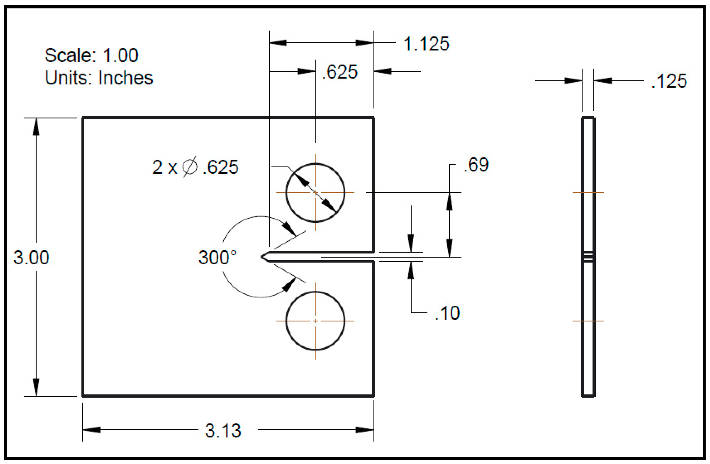
Figure 3.
Standard CT specimen with a mounted AE sensor.
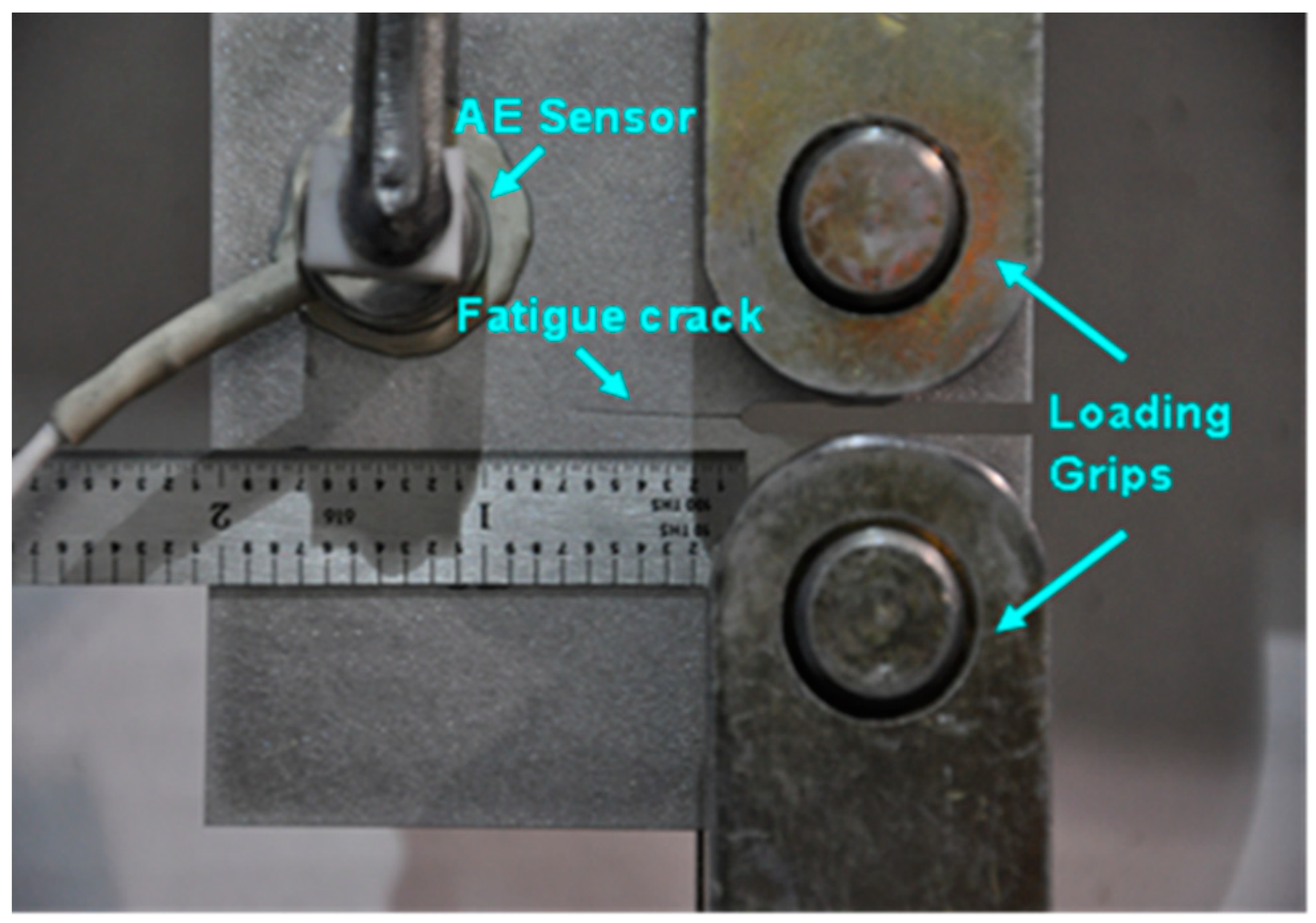
Figure 4.
Example of crack length measurements paired with cumulative AE counts.
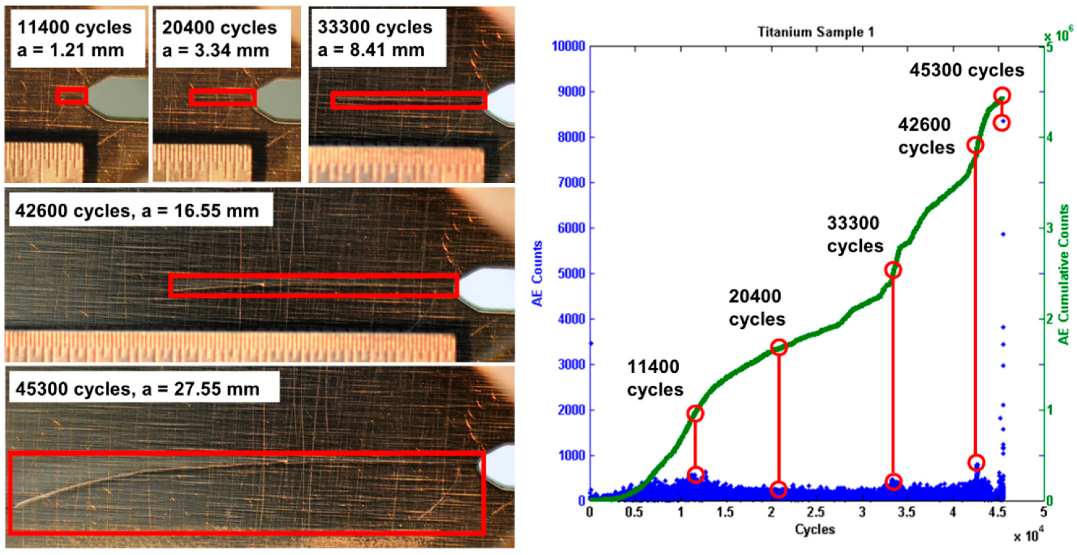
Figure 5.
Crack growth rate versus AE count rate for Al7075-T6 tests at (a) different loading ratios; (b) different loading frequencies—log scale. The base scale of da/dN is in/cycle.
Figure 5.
Crack growth rate versus AE count rate for Al7075-T6 tests at (a) different loading ratios; (b) different loading frequencies—log scale. The base scale of da/dN is in/cycle.

Figure 6.
Estimated error terms.
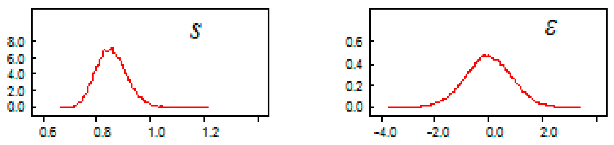
Figure 7.
Posterior predictive AE model with the uncertainty bounds, material: Al7075-T6; WB indicates Bayesian regression analysis results using WinBugs.
Figure 7.
Posterior predictive AE model with the uncertainty bounds, material: Al7075-T6; WB indicates Bayesian regression analysis results using WinBugs.

Figure 8.
Posterior predictive AE model with the uncertainty bounds, material: Ti-6Al-4V, WB indicates Bayesian regression analysis results using WinBugs.
Figure 8.
Posterior predictive AE model with the uncertainty bounds, material: Ti-6Al-4V, WB indicates Bayesian regression analysis results using WinBugs.

Figure 9.
Crack growth rate versus AE count rate with linear regressions for Al7075-T6 and Ti-6Al-4V.
Figure 9.
Crack growth rate versus AE count rate with linear regressions for Al7075-T6 and Ti-6Al-4V.
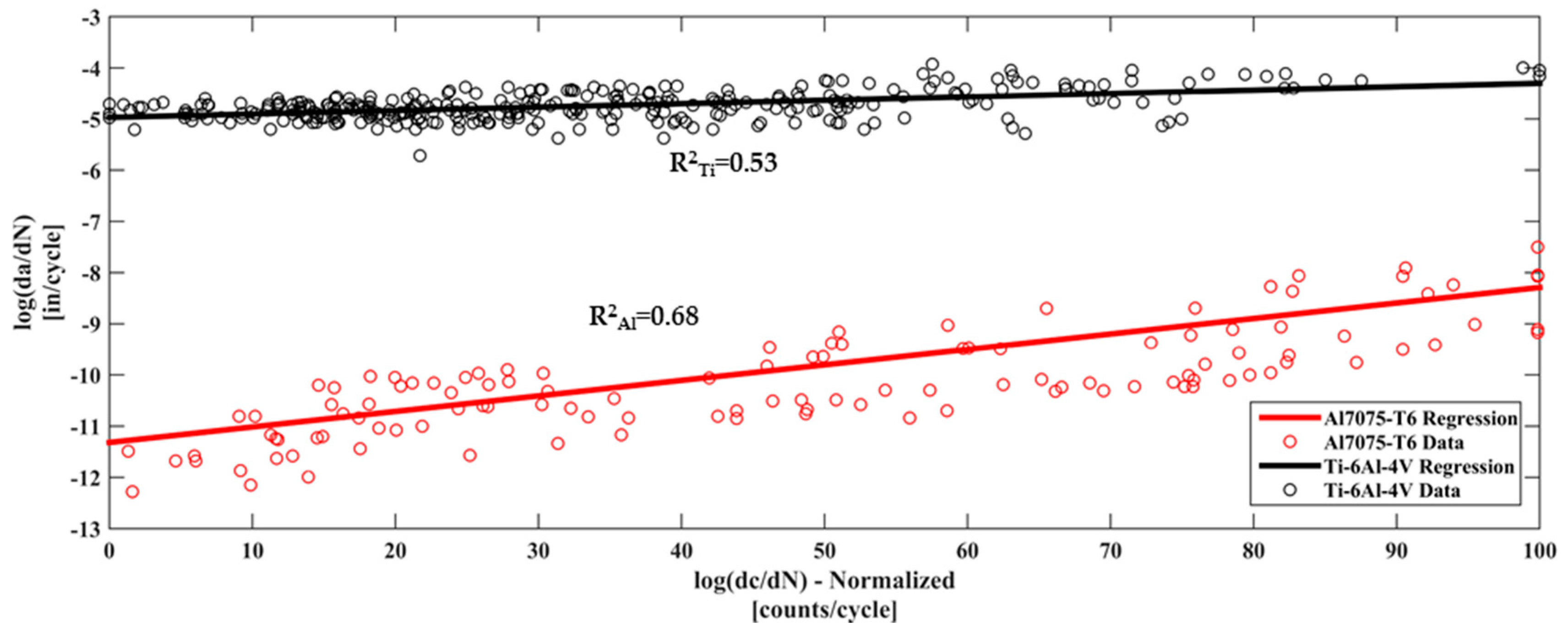
Figure 10.
Comparison of AE model prediction and experimental results (log da/dN). WB indicates Bayesian regression analysis results using WinBugs.
Figure 10.
Comparison of AE model prediction and experimental results (log da/dN). WB indicates Bayesian regression analysis results using WinBugs.


Table 1.
Details of experiments and load parameters.
| Test Reference | Material | Loading Frequency (Hz) | Loading Ratio | Maximum Force (lbf) | Maximum Force (kN) |
|---|---|---|---|---|---|
| CT1 | Al7075-T6 | 10 | 0.1 | 500 | 2.22 |
| CT2 | Al7075-T6 | 10 | 0.1 | 500 | 2.22 |
| CT3 | Al7075-T6 | 10 | 0.3 | 500 | 2.22 |
| CT4 | Al7075-T6 | 10 | 0.3 | 500 | 2.22 |
| CT5 | Al7075-T6 | 10 | 0.5 | 500 | 2.22 |
| CT6 | Al7075-T6 | 10 | 0.5 | 500 | 2.22 |
| CT7 | Al7075-T6 | 2 | 0.1 | 500 | 2.22 |
| CT8 | Al7075-T6 | 2 | 0.1 | 500 | 2.22 |
| CT9 | Al7075-T6 | 7 | 0.1 | 500 | 2.22 |
| CT10 | Al7075-T6 | 7 | 0.1 | 500 | 2.22 |
| CT11 | Al7075-T6 | 10 | 0.1 | 500 | 2.22 |
| CT12 | Al7075-T6 | 10 | 0.1 | 500 | 2.22 |
| CT13 | Ti-6Al-4V | 5 | 0.1 | 900 | 4 |
| CT14 | Ti-6Al-4V | 5 | 0.1 | 900 | 4 |
| CT15 | Ti-6Al-4V | 5 | 0.1 | 900 | 4 |
Table 2.
Regression parameters for individual test data, Al7075-T6.
| Test | Frequency | R | α1 | α2 |
|---|---|---|---|---|
| CT1 | 10 | 0.1 | 0.03 | −11.46 |
| CT2 | 10 | 0.1 | 0.03 | −11.17 |
| CT3 | 10 | 0.3 | 0.03 | −11.09 |
| CT4 | 10 | 0.3 | 0.02 | −12.01 |
| CT5 | 10 | 0.5 | 0.03 | −11.97 |
| CT6 | 10 | 0.5 | 0.02 | −11.77 |
| CT7 | 2 | 0.1 | 0.02 | −10.88 |
| CT8 | 2 | 0.1 | 0.05 | −13.86 |
| CT9 | 7 | 0.1 | 0.02 | −10.86 |
| CT10 | 7 | 0.1 | 0.02 | −10.74 |
| CT11 | 10 | 0.1 | 0.04 | −12.91 |
| CT12 | 10 | 0.1 | 0.04 | −13.41 |
Table 3.
Regression parameters and error term distribution for Al7075-T6 and Ti-6Al-4V tests.
| Material | α1 | α2 | ε ~ N(με,s) | s ~ N(μs,σs) | ||
|---|---|---|---|---|---|---|
| µε | μs | σs | ||||
| Al7075-T6 | 0.03 | −11.319 | 0 | 0.86 | 0.057 | |
| Ti-6Al-4V | 0.006 | −4.971 | 0 | 0.24 | 0.010 | |
Table 4.
Model validation statistic summary.
| Parameter | Mean | Standard Deviation | 2.5% | Median | 97.5% |
|---|---|---|---|---|---|
| bm | 0.009 | 0.011 | −0.013 | 0.009 | 0.031 |
| sm | 0.059 | 0.008 | 0.045 | 0.058 | 0.078 |
| Fm | 1.011 | 0.061 | 0.894 | 1.009 | 1.141 |
© 2018 by the authors. Licensee MDPI, Basel, Switzerland. This article is an open access article distributed under the terms and conditions of the Creative Commons Attribution (CC BY) license (http://creativecommons.org/licenses/by/4.0/).
Share and Cite
MDPI and ACS Style
Keshtgar, A.; Sauerbrunn, C.M.; Modarres, M. Structural Reliability Prediction Using Acoustic Emission-Based Modeling of Fatigue Crack Growth. Appl. Sci. 2018, 8, 1225. https://doi.org/10.3390/app8081225
AMA Style
Keshtgar A, Sauerbrunn CM, Modarres M. Structural Reliability Prediction Using Acoustic Emission-Based Modeling of Fatigue Crack Growth. Applied Sciences. 2018; 8(8):1225. https://doi.org/10.3390/app8081225
Chicago/Turabian StyleKeshtgar, Azadeh, Christine M. Sauerbrunn, and Mohammad Modarres. 2018. "Structural Reliability Prediction Using Acoustic Emission-Based Modeling of Fatigue Crack Growth" Applied Sciences 8, no. 8: 1225. https://doi.org/10.3390/app8081225
Note that from the first issue of 2016, this journal uses article numbers instead of page numbers. See further details here.