Effect of the Temporal Gradient of Vegetation Indices on Early-Season Wheat Classification Using the Random Forest Classifier

1
Department of Photogrammetry and Remote Sensing, Faculty of Geodesy & Geomatics Engineering, K. N. Toosi University of Technology, Tehran 19967-15433, Iran
2
AgriWatch BV, Weerninklanden 24, 7542 SC Enschede, The Netherlands
3
Department of Geomatics, School of Civil Engineering, Iran University of Science and Technology, Tehran 16846-13114, Iran
*
Author to whom correspondence should be addressed.
Appl. Sci. 2018, 8(8), 1216; https://doi.org/10.3390/app8081216
Submission received: 27 May 2018
/
Revised: 19 July 2018
/
Accepted: 20 July 2018
/
Published: 24 July 2018
(This article belongs to the Special Issue Selected Papers from The 4th China International Agricultural Remote Sensing Application and Technology Summit (ARS 2018))
Abstract
:Early-season area estimation of the winter wheat crop as a strategic product is important for decision-makers. Multi-temporal images are the best tool to measure early-season winter wheat crops, but there are issues with classification. Classification of multi-temporal images is affected by factors such as training sample size, temporal resolution, vegetation index (VI) type, temporal gradient of spectral bands and VIs, classifiers, and values missed under cloudy conditions. This study addresses the effect of the temporal resolution and VIs, along with the spectral and VIs gradient on the random forest (RF) classifier when missing data occurs in multi-temporal images. To investigate the appropriate temporal resolution for image acquisition, a study area is selected on an overlapping area between two Landsat Data Continuity Mission (LDCM) paths. In the proposed method, the missing data from cloudy pixels are retrieved using the average of the k-nearest cloudless pixels in the feature space. Next, multi-temporal image analysis is performed by considering different scenarios provided by decision-makers for the desired crop types, which should be extracted early in the season in the study areas. The classification results obtained by RF improved by 2.2% when the temporally-missing data were retrieved using the proposed method. Moreover, the experimental results demonstrated that when the temporal resolution of Landsat-8 is increased to one week, the classification task can be conducted earlier with slightly better overall accuracy (OA) and kappa values. The effect of incorporating VIs along with the temporal gradients of spectral bands and VIs into the RF classifier improved the OA by 3.1% and the kappa value by 6.6%, on average. The results show that if only three optimum images from seasonal changes in crops are available, the temporal gradient of the VIs and spectral bands becomes the primary tool available for discriminating wheat from barley. The results also showed that if wheat and barley are considered as single class versus other classes, with the use of images associated with 162 and 163 paths, both crops can be classified in March (at the beginning of the growth stage) with an overall accuracy of 97.1% and kappa coefficient of 93.5%.
1. Introduction
The global demand for food will increase due to the growth of the global population over the course of this century [1]. It is, therefore, necessary to accurately estimate the crop area to determine if the demand for food can be met [2]. Farmers usually decide to change the crop type of their agricultural fields in response to the regional demand and drought conditions. Therefore, the cultivated area of a given crop alters from one growing season to the next. Consequently, early-season crop area forecasting, in particular for wheat crops, is essential information for policy-makers to manage yields for domestic use, imports, or exports.
The classification of remotely-sensed data can provide the regional distribution of individual crop types for government agencies [3,4] and decision-makers of the commodity trade. Evidently, the classification of agricultural crops using only one image captured at a given date has significant shortcomings [5]. Firstly, the crop types may have different growth stages and, secondly, different crops may have similar spectra (e.g., wheat and barley in this case study) during the growing season in a complex agricultural area [6]. It is, therefore, difficult to distinguish crop types at a certain point in the growth period by an image at a given time [7]. In contrast, multi-temporal images provide temporal signatures of crops and represent the growth period by capturing data during the growing season [8]. A significant advantage of using multi-temporal data is that the proportions of different crop types can be differentiated using the spectral differences at different points in the growing season [9,10,11,12,13]. Recently, crop areas from non-crop areas have been separated by detecting changes in greenness using the time-series normalized difference vegetation index (NDVI) data in Reference [14]. Moreover, an approach based on object-based NDVI time series analysis is used for regional-scale mapping of agricultural land-use systems [15]. The crop area in the early season was also determined using the enhanced vegetation index (EVI) of the multi-temporal Moderate Resolution Imaging Spectroradiometer (MODIS) in References [10,16]. In their study, the green-up rate of the crop canopy, i.e., the accumulated difference of two consecutive images, is used. The obtained results indicated that multi-temporal remote sensing approach could be used with confidence in early-season crop area prediction at least one to two months ahead of anthesis. Moreover, with an increasing number of images, applying different vegetation indexes (VIs) and their differences, the training sample size increases dramatically to overcome the limitation of dimensionality for supervised classification [17]. In the study done by Reference [18], different data types, including reflectance data, spectral indices, texture indices, and Digital Earth Model (DEM) features, are used in a combined random forest (RF) and object bases image analysis scheme for agricultural area mapping. However, these approaches require cloud-free imagery and processing of multiple images is prohibitive for operational implementation over large areas. In this regard, acquiring such frequent cloud-free imagery is a serious limitation in estimating crop area [19,20].
Indeed, classification of multi-temporal images is a challenging task that is affected by many factors that limit the accuracy. In particular, these issues include appropriate training sample size, revisit time, as well as suitable VIs. The effect of these factors also depends on the choice of the classifier [21]. Some studies have been done to address some of these issues [22,23,24,25]. For example, the optimal number and dates of images for land cover classification are identified with feature importance obtained by RF classifier on remote sensing time-series [26]. In another study the sensitivity of the RF classification to select training sample points, including sample size, spatial autocorrelation, and proportions of classes within the training sample were investigated [24]. The effect of the time series length on crop mapping is investigated. In that study, RF is used to calculate the important scores for VIs and the Jeffries–Matusita (JM) distance is used to measure class separability for each time series [27]. In a comprehensive study, five classifiers that can also be applied to high-resolution multi-temporal optical imagery to produce accurate crop type maps have been selected and benchmarked at the global scale [28]. These classifiers are RF, support vector machine (SVM) with a radial basis function kernel, Dempster–Shafer fusion of the previous approaches, best classifier with a mean-shift smoothing, and best classifier with a temporal regular resampling. The obtained classification results on the 12 test sites around the globe demonstrated that RF achieved superior results. The RF is also used for winter wheat mapping by multi-temporal images of LDCM and Gao Fen 1 satellites [29].
Liu et al. [29] prepared the wheat map by combining multi-temporal and multi-source data using the random forest classifier. They used six images during the wheat growth stages and two NDVI and Soil Adjusted Vegetation Index (SAVI) for each image. The input features of the RF were 36 spectral bands and 12 vegetation indices in a total of 48 features. They classified two classes and separated the wheat from non-wheat. They performed classification with an overall accuracy of 92.9% and a kappa coefficient of 85.8%. However, they did not report in their study whether they considered barley in the wheat class or non-wheat class. Khan et al. [30] also classified two wheat and non-wheat classes by analyzing Landsat images in Pakistan’s Punjab region with the supervised bagged classification tree approach and reached an overall accuracy of 76%. They did not also mention the barley class. Inglada et al. [31] using Landsat time-series images and Synthesis Aperture Radar (SAR), conducting early crop type identification and considering two classes of wheat and barley in one class and, in the best case, using seven Sentinel-1 images and nine Landsat-8 images, the kappa coefficient κ = 0.73 was obtained. However, the VI information was not used in their study. Fletcher [23] introduced vegetation indices as new features in the random forest for the classification of soybeans and weeds and confirmed the positive effect of vegetation indices, and the overall accuracy of 90.8% and the kappa coefficient of 0.878 were obtained using the image (30 June 2014). Zheng et al. [14] classified various types of crops by using a support vector machine classifier using the NDVI time series data that was extracted from Landsat images. They considered the wheat and barley classes separately and reported an overall accuracy of 90% and a kappa coefficient of 85%. They also reported that the producer’s accuracy of the wheat was 67% and the user’s accuracy was 53%. Nitze et al. [26] compared four types of support vector machine, artificial intelligence network, random forest, and maximum likelihood in order to classify various types of crops and defined two barley and wheat classes separately, and with the use of only spectral band information from three images, the producer’s accuracy for wheat and barley of 79.7% and 70.8%, respectively, were obtained. Allen et al. [3] classified the crops of the United States using multi-source data by the supervised decision tree classifier and obtained an overall accuracy and kappa coefficient of 91.65 and 0.8618, respectively. They used only the spectral band of images and the producer’ accuracy of the wheat and barley were reported to be, respectively, 90.72% and 15.73%.
In the aforementioned circumstances, the study of the optimal number of images to find the critical image acquisition times and temporal resolution along with VIs and their gradient is necessary. This paper will address the issue of how important the temporal resolution of image acquisition for multi-temporal image classification is and what happen when the temporal resolution of Landsat-8 increases to one week. For this purpose, the study area selected is an overlapping area between two Landsat paths. Moreover, missing data problems due to cloudiness is another matter which limits the application of multi-temporal image classification. Indeed, many training pixels or test data are ignored if only one cloudy image exists in the time series. Although considerable research has been previously done on the time-series classification, the problem of missing data caused by cloudy pixels in such images is still an issue to which less attention has been paid. One of the main problems in multi-temporal image classification is that some pixels of training/test areas may be covered by cloud. Hence, those pixels are ignored and neither incorporated as training data in the classifier learning process nor as test data for the classification accuracy. This paper remedies this problem for those cloudy pixels, retrieves the missing data through k-nearest cloudless pixels in the feature space and investigate effect of missing data retrieved on the classification results of multi-temporal images.
This paper also addresses the impact of the appropriate image acquisition times and VIs along with the spectral and VIs gradient on the RF classifier when missing data exist in the multi-temporal images. The objective of this paper is, therefore, to investigate the practical considerations of the multi-temporal image classification approach for consultants and agronomists. The specific goals of this study are: (1) to assess the effect of missing data in training areas, due to being cloudy, on RF classification learning; (2) to determine the appropriate data acquisition times and temporal resolution; (3) to assess the effect of VIs and their temporal gradient along with temporal gradient of spectral bands in different times; and (4) to determine the optimum number of classes to be distinguished in the early season. To our knowledge, there are currently no other comprehensive assessments of multi-temporal image classification which takes into consideration these practical aspects. We proposed a developed method for image time series processing that improves the classification of winter wheat results even in early crop classification.
2. Materials and Methods
2.1. Study Area and Data
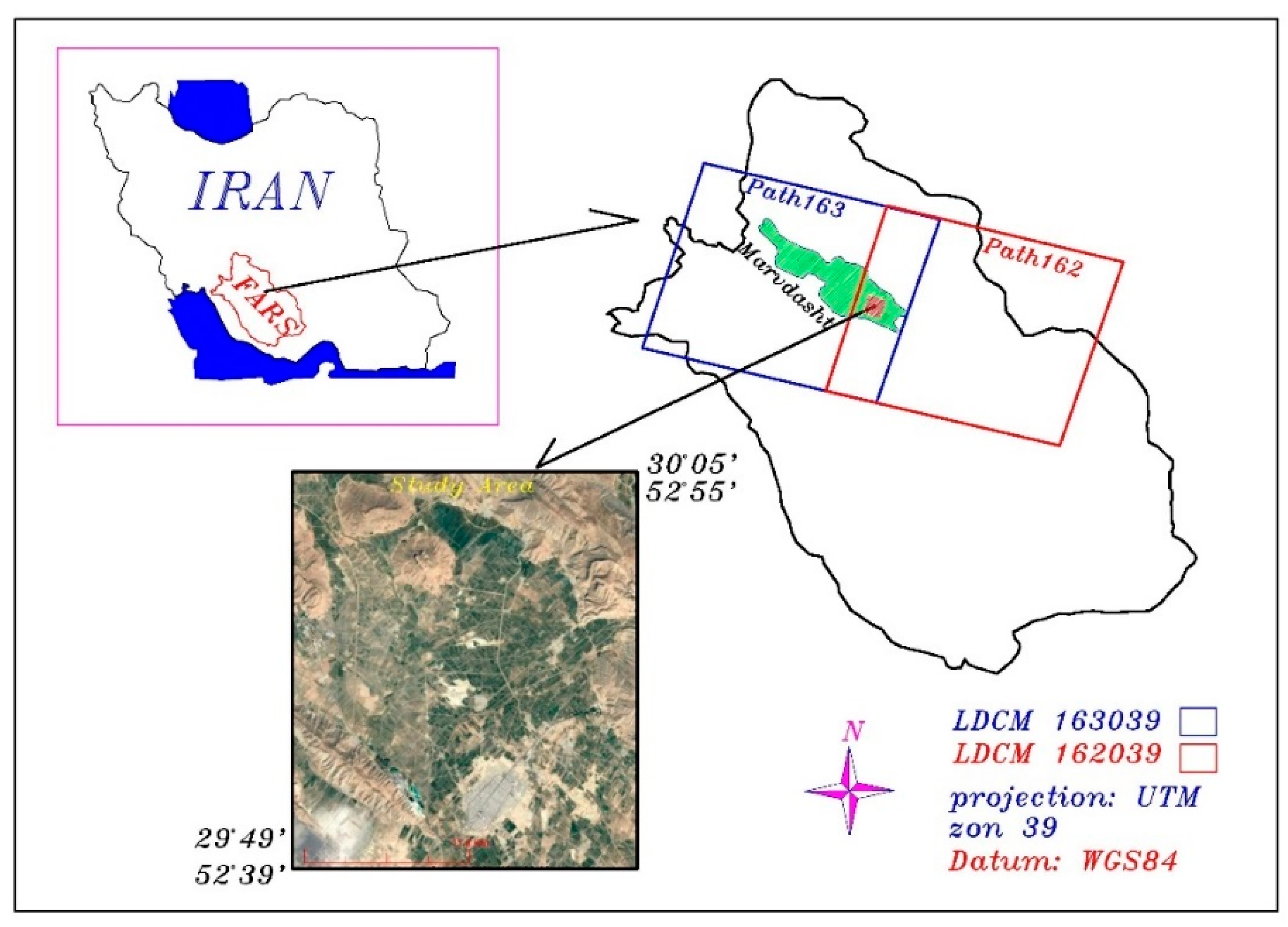
The study area is an agricultural region with an area of 755 km2, located between latitudes 29°49′–30°05′ N and longitudes 52°39′–52°55′ E, in Southwest Iran (Figure 1). The area has various climates during the growing season and is covered by different vegetation, soil, and rocky terrain types. Marvdasht is located 45 km north of Shiraz with an altitude of 1620 m above sea level and an area of 4649 km2. In the month of August, precipitation is at its lowest, with an average of zero millimeters. The highest precipitation rate occurs in January, with an average about 71 mm and the total annual precipitation is about 516 mm, in the study area. July is the hottest month, with an average temperature about 28.4 °C. January is the coldest month, with an average temperature of about 5.4 °C. Between the driest and most humid months of the year, the precipitation difference is about 71 mm, and during the year the temperature varies by 23.0 °C. According to the de Martonne index (10 < I < 19.9), this region is considered as a semi-arid climate region of Iran.
The images used in this research are obtained from LANDSAT-8 satellite images. The spatial resolutions of the images of bands 1–7, as well as band 9 of the LANDSAT-8 images, are 30 m and band 8 (panchromatic band) is 15 m, while bands 10 and 11 are thermal bands with a spatial resolution of 100 m, which has been resampled to the pixel size of 30 m. In this study, by inserting sensor and image parameters, such as the zenith angle of the sun at the image acquisition time, the azimuth angle of the sun and the sensor, the date and image acquisition time, and the size of pixels, etc., atmospheric and radiometric corrections were performed using ATCOR IDL-based Atmospheric and Topographic Correction software [32].
The study area is situated on an overlapping area between paths 162 and 163, which is covered by 21 scenes of LDCM data captured from 11 January 2015 until 20 June 15 during the growing season. Among all images, 10 images with an amount of cloudiness less than 20% in their metadata were selected, of which eight images belonged to path 162 and two images to path 163. The acquisition times of these images are given in Table 1.
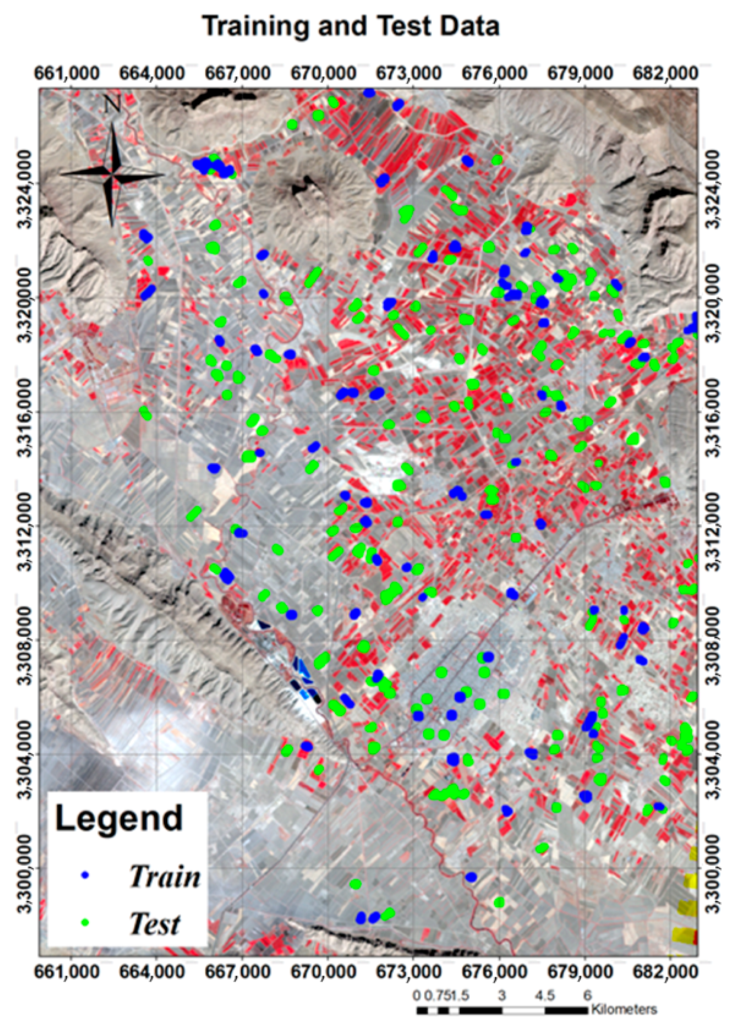
The training and test data used in this research were obtained from the Ministry of Agriculture Jihad of Iran, which was taken by the direct field working method. A total of 847 farms, including 408 wheat fields, 66 barley farms, and 373 farms of other classes, were provided to us as data of known class. Among these data, 128 wheat farms, 15 barley farms, and 121 other-class farms were selected as training data and the rest were selected as independent testing data not included in the classification (Table 2). Approximately five pure pixels from the center of each farm were extracted as a representative of that class, classification was performed with the training data, and validation was performed with independent test data. In Figure 2, the training data and their dispersion have been shown with blue points and validation data are specified with green points.
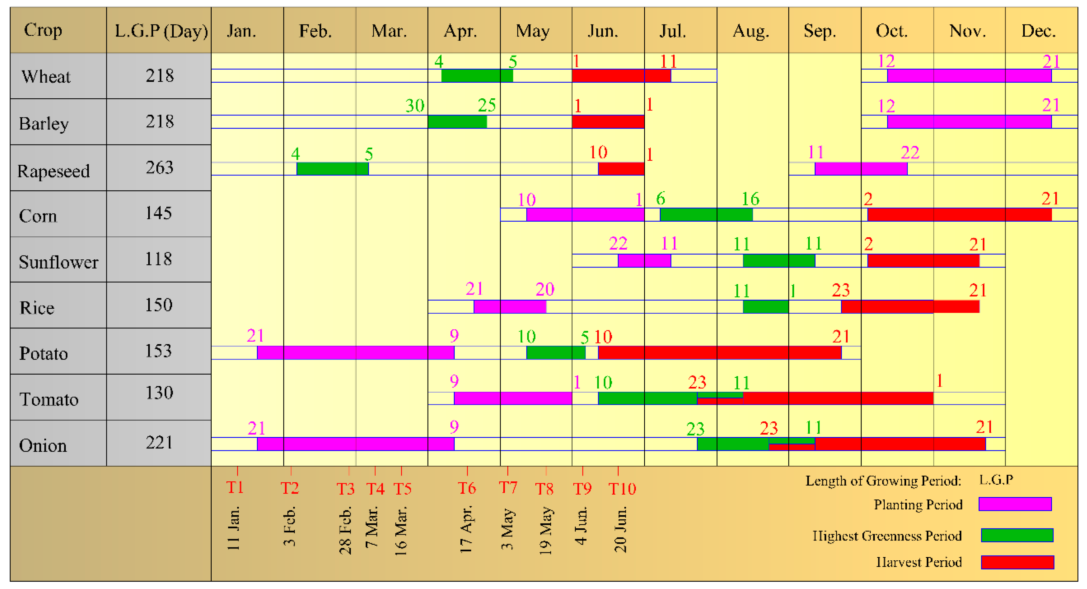
The main crops of the study area are wheat, barley, corn, rapeseed, sunflower, rice, potatoes, tomatoes, and onions. Figure 3 shows the general agronomic calendars of the crops in the study area. As shown in Figure 3, wheat and barley are planted between 12 October and 21 December, and the difference in the time needed to attain the peak between these two crops’ greenness. Barley reaches its greenness peak slightly earlier than wheat, and tends to become yellowish earlier than wheat [33].
2.2. Methodology
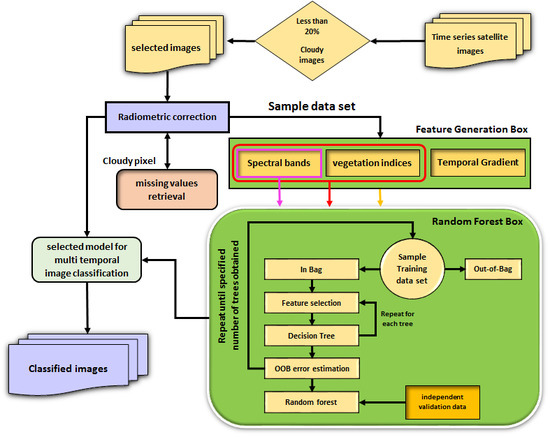
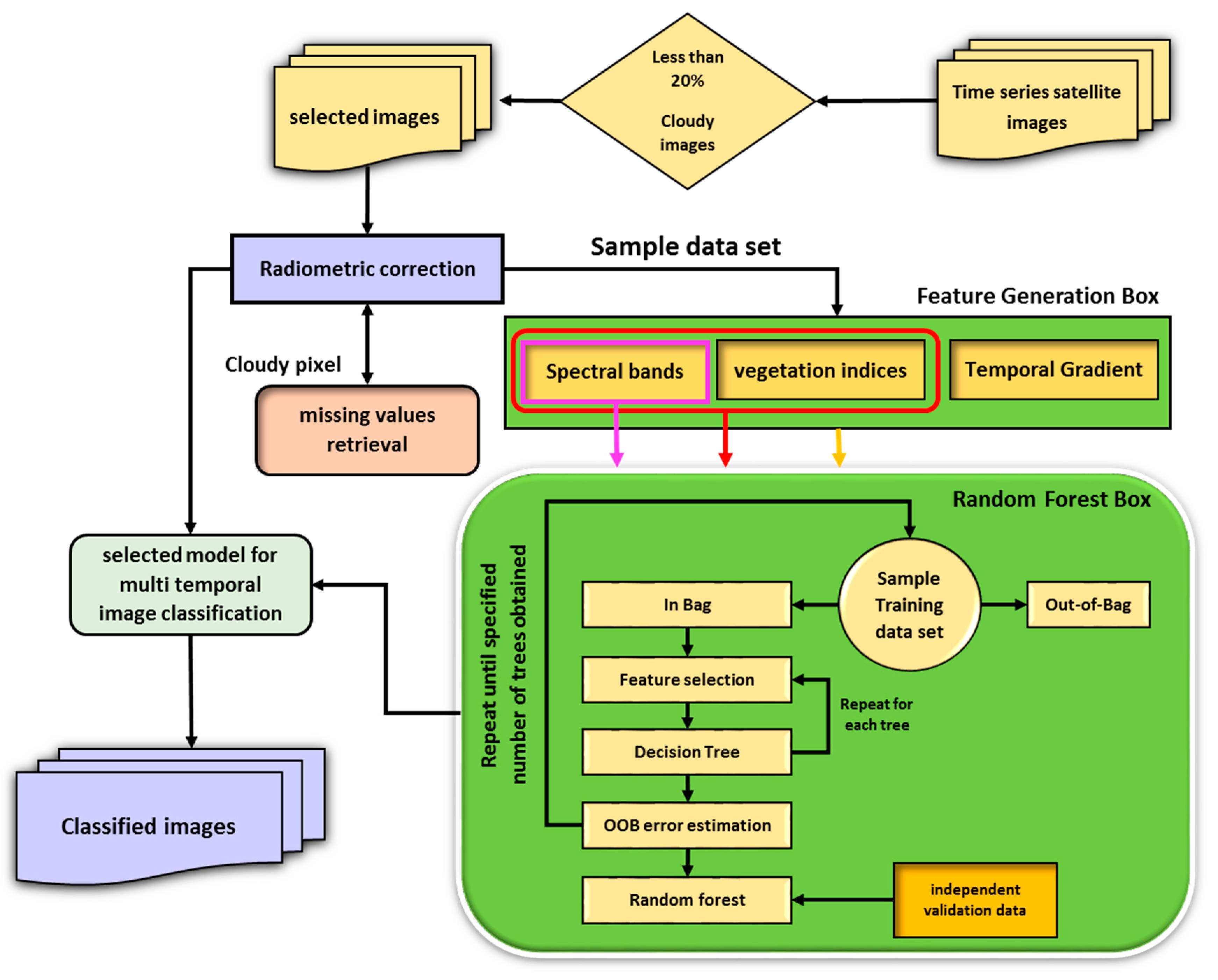
As mentioned above, the classification of multi-temporal images is affected by many factors, such as missing data in cloudy images, optimum training sample size, and appropriate temporal resolution for image acquisition that limits the accuracy. Moreover, extraction of appropriate features (e.g., the temporal gradient) from the temporal signatures of crop types, along with suitable times such that differentiate crops are two major issues that should be considered in the multi-temporal image classification. In this regard, different features, like VIs, the temporal gradient of VIs, and spectral bands, are taken into account as new features. To address the aforementioned issues, we developed the following methodology (Figure 4).
Step 1: A set of images with an amount of cloudiness less than 20% in their metadata, were selected from input time-series images. Radiometric correction is then applied to the selected images (i.e., 10 images for this study area) and cloudy pixels in each image are set to no data as missing data for all bands. Hence, for each pixel, a feature vector with a dimension of 80 elements (8 × 10) is achieved.
Step 2: As can be seen in Figure 4, the missing data retrieval is a preprocessing task before RF classification. Indeed, the missing data of pixels due to cloudy periods are very important, since many pixels are ignored during multi-temporal image classification. The proposed method for missing data retrieval is described in detail in Figure 5.
Step 3: After missing data retrieval, the VIs are generated. Previous studies have not investigated the impact of VIs on classification of wheat, but it is clear that RF was most effective at detecting them. In the current study nine indices, are computed based on the corresponding equations listed in Table 3, as new features. The goal of considering 9 VIs is to create features that enhance classification accuracy.
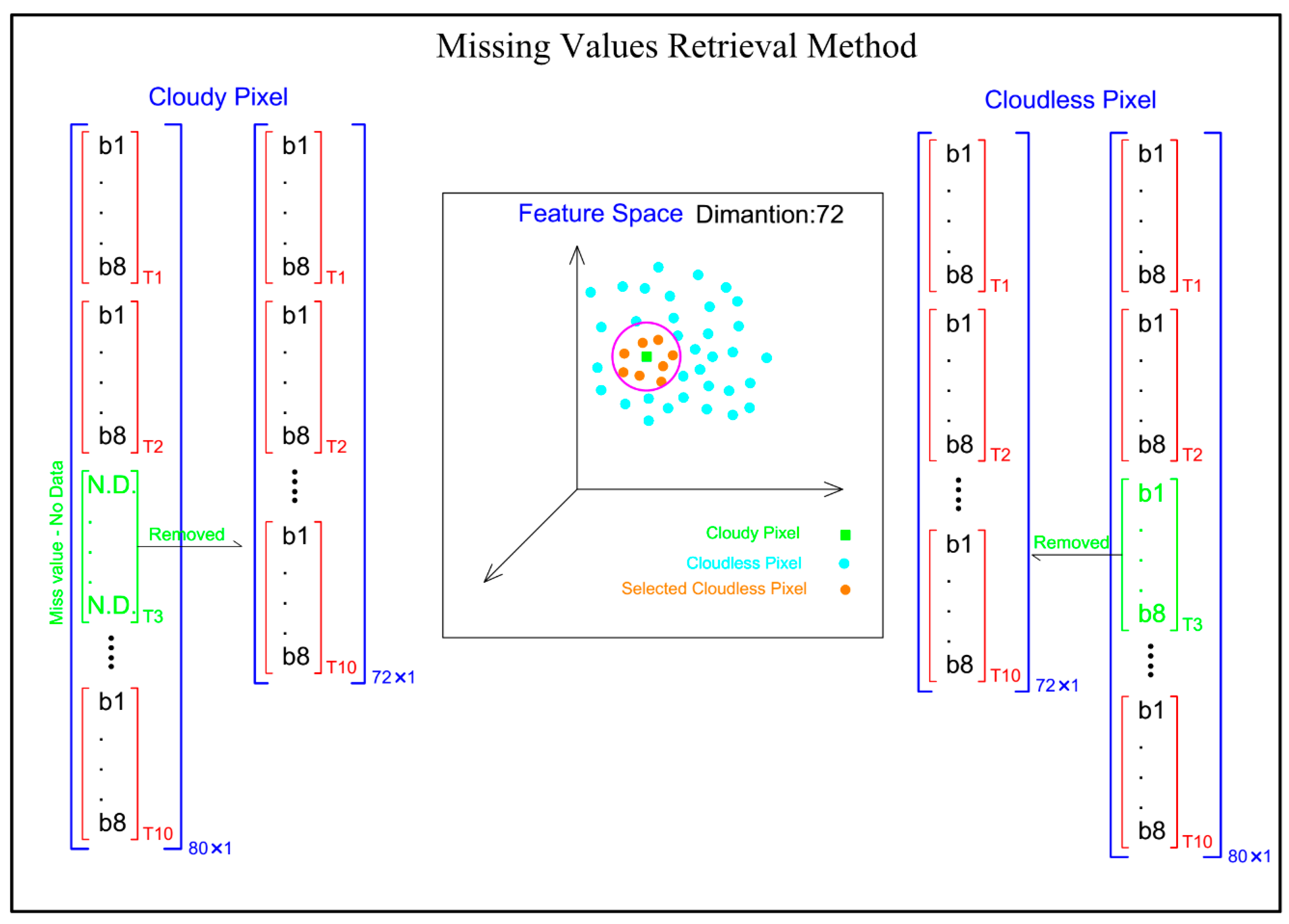
To retrieve the missing data, all the bands of a pixel corresponding to cloudy periods in a given training/test data set (i.e., wheat) that contain no data were removed from the feature vector (i.e., an image which captured in time 3) and flagged as cloudy pixels. The corresponding bands from the feature vector of the cloudless pixels of that class were also removed (i.e., the corresponding bands of cloudy times are removed in cloudless pixels of that class) to obtain the same dimensionality with the cloudy pixels (i.e., 72 × 1). In the reduced multi-dimensional feature space, for each cloudy pixel (i.e., the. green pixel in Figure 5), k-nearest cloudless pixels (i.e., the red pixels in Figure 5) are then found. Therefore, the bands of pixels with no data were reconstructed using the mean of the k-nearest neighbor cloudless pixels, to obtain a feature vector with full dimensionality. In other words, the missing data of cloudy pixel bands are filled with the mean of the k-nearest cloudless pixels, which are spectrally similar to cloudy pixels in the feature space. This was also applied for all of the cloudy pixels of the scene after the appropriate multi-temporal classification model was selected.
Step 4: Since the temporal signature plays an important role in the interpretation of the growing steps of crops, a temporal gradient is used to quantitatively describe the seasonal change. The temporal gradient of a given spectral band, TGSB, at the ith () and jth () times are then generated to obtain the temporal changes of crops as follows:
The temporal gradients of VIs, TGVI, are also computed and considered as new features, which means for a given VI at the ith () and jth () times, a set of VI gradients in time sequence is generated as follows:
Step 5: The RF algorithm is implemented to explore the achieved features, including spectral bands at different times, VIs, and their temporal gradients, to obtain an ensemble of decision trees. As mentioned, eight images from path 162 and two images from path 163, having less than 20% cloud cover, are selected. Therefore, for each pixel, a feature vector is obtained that includes spectral bands and VIs, along with their temporal gradients. To investigate the effect of multi-temporal image classification issues by the RF classification, different scenarios are considered according to Table 4.
The RF algorithm can generally handle high dimensional data and use a large number of trees in the ensemble. In RF, each tree in the forest is built and tested independently from other trees. During training, each tree receives a new bootstrapped training set generated from the original training set by subsampling with a replacement [43]. Those samples which are not included during the training of a tree are called out-of-bag (OOB) samples of that tree. These samples can be used to compute the out-of-bag-error (OOBE) of the tree, as well as the ensemble, which is an unbiased estimate of the generalization error [44,45,46].
In the experiments, replacement and OOB are set to 15 times and 33%, respectively. First, the optimum number of training sample size along with the number of trees are investigated. Then, the effect of each other items in Table 4 issue is assessed to obtain an appropriate model for the multi-temporal classification.
Decision-makers aim to measure the crop area from remotely-sensed data in earlier seasons with appropriate accuracy. Therefore, according to Table 5, based on the desired classes, two cases of classification are determined by the decision-makers.
3. Results and Discussion
3.1. Experiment 1: Optimum Training Sample Size
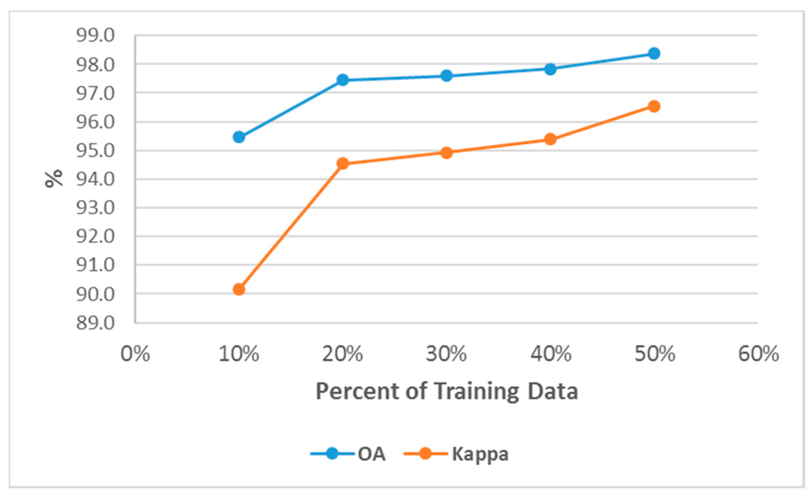
In this experiment the sample size of the training data, set to 10% up to 50% without considering missing data and only spectral bands of eight images captured on path 162, without their gradient and VIs, are used for classification. The RF classification is performed with 15 times replacement and with 50 trees (forest size) in case 1. The averages of the overall accuracy (OA) and kappa coefficient [47] are computed and provided in Figure 6.
With an increasing training sample size, the OA and the kappa coefficient are improved (Figure 6). This improvement is not remarkable when the training sample size becomes more than 30%. Hence, we selected 30% as the appropriate training size due to the cost of fieldwork.
3.2. Experiment 2: Optimum Forest Size
Most of the experiments using RF classification are done with a large number of trees, which is time consuming [27,48]. The default tree number of 200–1000 used in some investigations greatly increases the computation cost [6]. Hence, the optimum forest size for each dataset should be investigated and determined. For this purpose, after measuring the optimum sample size in experiment 1, the optimum forest size is also investigated through increasing trees from 10 up to 1000 trees to reduce the time of further calculations. In this experiment, the RF classification is also conducted with 15 times replacement in case 1 using only the spectral bands of all images. As shown in Figure 7, the overall accuracy and kappa coefficient were increased by less than 1% after 50 trees, up to 1000 trees, but instead, the computation time increased from 165 s to 2176 s (Table 6). Thus, the number of optimal trees in this experiment was set to 50.
Table 6 shows the processing time of each RF classifier implementation. As can be seen, by increasing the number of trees, required time for each run increases linearly.
3.3. Experiment 3: The Effect of Missing Data in the Training Data
In fact, due to probable presence of clouds in some of the images, information was not available for cloudy pixels in the classification of multi-temporal images if these cloudy pixels are removed. Thus, cloudy pixel data, as missing data, will not participate in the classification process. Retrieval of missing data in images, such as plant greenness peak images, which play a major role in the classification, is of particular importance and provides information used for classification that is closer to reality. As described in Step 2 of the Methodology section, all cloudy pixels in training and testing data were retrieved by the k-nearest method and then classified. Table 7 provides classification results in the case of eliminating missing data and also in the retrieval mode, then the retrieved pixels were employed in the RF classifier process. The overall accuracy in the retrieval of missing values is 95.4%, and in the absence of missing data is 93.2%. The results show an increase of 2.2% overall accuracy and, in total, the improvement of classification results in the retrieval mode of missing data in the feature space. It should be noted that all time-series images were used in this experiment and k was set as 7 in this study.
3.4. Experiment 4: Appropriate Image Acquisition Times and Temporal Resolution
One of the challenges in using multi-temporal data is to provide early information about the cultivation area and crop types for decision-makers with a few images. Hence, at first, only different sequential times of path 162 were selected to assess which image acquisition times were suitable for early classification. Then classification was done on case 1 using different combinations of acquisition time sequences. The summary of using eight combinations of image acquisition times that obtain acceptable results are given in Table 8.
The best combination, with regards to wheat and barley separation in terms of early detection and high accuracy, as well as optimum images, is the use of T1 (planting period of wheat and barley), T6 (highest greenness of wheat and barley), and T7 (barley tends to become yellowish but wheat is still green) images (Table 8). However, if only the parameter “minimum number of images”, regardless of the producer accuracy of the barley, is considered, combination 7 represents the best results. In order to show the effect of the temporal resolution on the accuracy since, after 16 March, the image without cloud on path 163 was not available, it is proper to examine the effect of increasing the temporal resolution to the extent of this date because the impact of the use of the May images will be high due to the closeness to the high crop greenness and will affect the temporal resolution effects.
Some of the pervious researches used MODIS time-series for temporal optimization of image acquisition [26]. In this research to demonstrate the effect of increasing the temporal resolution of the LDCM to one week, the images of path 163 (i.e., dates 03-FEB-15 and 07-MAR-15) are incorporated into the experiment. Therefore, to compare the effects of the temporal resolution, combinations 6 and 10 were compared. As shown in Table 8, if the T1, T3, and T5 images (i.e., Comb. 6) are used, the overall accuracy and kappa coefficients will be 86.8% and 71.5%, respectively. If the Landsat temporal resolution is reduced to one week, then the T2 and T4 images can be used and, according to combination 10, better results are obtained in less time. In other words, if the time resolution of Landsat’s images is increased to one week, it can have better results. Of course, it is necessary to consider that by increasing the temporal resolution of the images to a week, especially when image acquisition times are near the peak of greenness of the crop, the probability of availability and obtaining images without cloud will be higher.
3.5. Experiment 5: The Effect of VIs and Their Gradient
This experiment aims to demonstrate the effect of VIs and their gradients on the classification accuracy improvement and their capabilities to decrease the scheduled time for image acquisition. For this purpose, firstly, NDVI and EVI, as examples of VIs, are considered and temporal signatures of wheat and barley are computed and depicted in Figure 8 for training data. In Figure 8a,c, the temporal gradient of NDVI and EVI for wheat and barley are showed. These diagrams may seem very similar in appearance, but the direction and size of their variations are different from time to time. In contrast to wheat, barley yields faster and loses its chlorophyll almost three weeks earlier. Then, the temporal gradient of wheat and barley is computed and given in Figure 8b,d. Although the temporal signatures of these crops in the first stages of growth are almost the same and have high spectral similarity, as shown in Figure 8, the temporal gradient at the end of the season can provide appropriate features for better discrimination. In particular, the temporal gradient between images T6 and T7, which were acquired on 17 April and 3 May, respectively, could provide the first significant difference between these similar classes for discrimination. In other words, from 17 April to 3 May, the wheat stands at the late stage of its growth, while the barley lost chlorophyll more rapidly.
In this research, because of the time series images used, the information from all plant growth stages was used as new features in the model. Since other crops in the area have a planting time, greenness peak time, and different harvest time, therefore, the spectral gradients and changes in their VIs will also be different. The proposed method performed well in distinguishing and classifying other crops. The main problem was the separation of wheat from the barley due to its similarity with the general agronomic calendar and the spectral similarity of the two crops.
In Figure 8a,b, the temporal gradient of NDVI shows that the barley greenness peak time was at T6 and, since then, the slope of the variation of the VI has been descending and, for wheat, it continues to rise until T7. The random forest distinguished between the two crops well using the same difference.
After illustrating the VIs and their temporal gradients, the gradient of spectral bands and the aforementioned VIs (Table 3) along with their temporal gradients (i.e., Equations (1) and (2)) are incorporated in the RF classification. Figure 9a,b, show the results obtained for 27 combinations of image acquisition times when only spectral bands are used. In addition to spectral bands, the effect of incorporating VIs and their spectral gradients obtained by Equations (1) and (2) are given in Figure 9a,b, in terms of OA and kappa coefficients. As demonstrated in Figure 9, by utilizing the temporal gradient of spectral bands and VIs, along with their gradients, the OA and kappa values are improved up to 5% and 9%, respectively.
The results of all of the various combinations of images are shown in Figure 9a,b. In the first case, only the T7 image was used and the overall accuracy and kappa coefficient were 92% and 82.9%, respectively. If any of the images are used, the results will be weaker until 17 April. For example, the results of using the T6 image for overall accuracy and the kappa coefficient were 79.9% and 58%, respectively. In the case in which only two images of time series images were used, T1 and T7 images had better results. In the case in which three images were used, T1, T6, and T7 had the best results. In addition to reducing the calculation time, as well as using the minimum number of images, this combination also provides the highest producer’s accuracy for barley (Table 9).
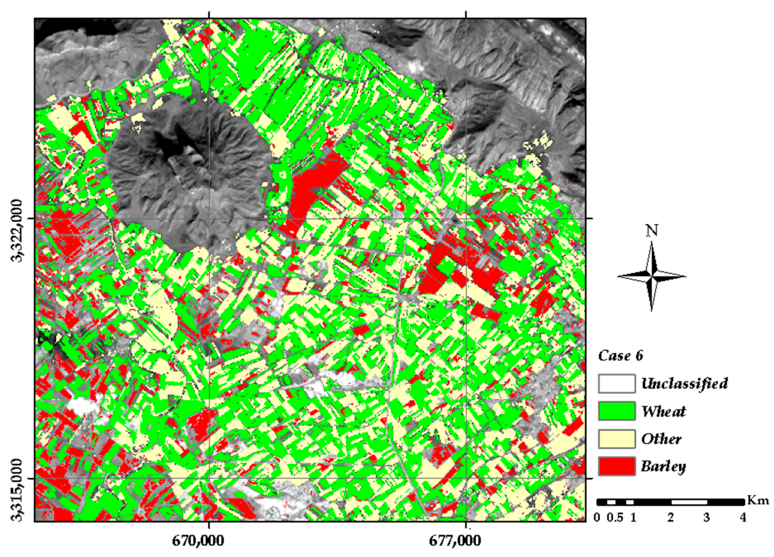
As shown in Table 9 when only spectral bands are used, there are 24 features. This number is 51 when only VIs are used. If gradient of VIs and gradient of spectral bands are added, the number of features increase to 102. Processing time column in Table 9 shows that the addition of new features imposes a low-cost computation. From 27 combinations, three combinations which incorporate the minimum acceptable number of images such that differentiate classes of case 1 early in the season are selected for comparison. In this experiment, classification was first done using only a spectral band data of images. Then vegetation indices were added to the model alone as a new feature, and it was observed that, by creating these features, the overall accuracy and kappa coefficient were improved by 1.3% and 2.4%, respectively. In the next step, in addition to the vegetation indices, the TGVI was added to the model as new features and it was observed that the overall accuracy and kappa coefficient were improved by 1.8% and 4.2%, respectively. In other words, the production of these new features increased the overall accuracy and kappa coefficient by 3.1% and 6.6% on average, respectively, compared to the conventional methods used to date. Most importantly, the barley producer’s accuracy, which has been reported in the other researches so far [4,26] and in the case of using only the spectral bands of images, showed a maximum around 70%, but using the proposed method and, in the case of using the optimized images, the separation capacity of barley from wheat and other crops was increased by 45.5%, reaching 92.5%. Figure 10 shows the classification map of the time series images of the studied area according to the optimal conditions in row 6 from Table 7.
In contrast to Comb. 4, in Comb. 3 the TGVI and TGBS do not improve the PA of barley significantly. This is due to the similarity between wheat and barley in the early stages of growth. Therefore, the results demonstrated that the appropriate model is Comb. 6, which utilizes only one image from the first stage of the growing season and two images from the seasonal change point of wheat and barley. It is worth noting that compared to Comb. 3, the scheduled time decreases to 07-MAR-15 in Comb. 7 and yields better results in terms of OA and kappa when the temporal resolution increases to one week (i.e., two images of path 163 are used).
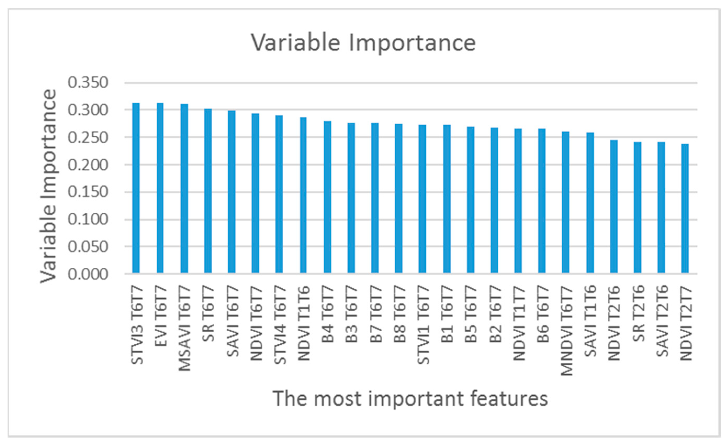
In the random forest, in order to estimate the importance of the mth variable of tree k, by eliminating the relevant variable, the decrease of the degree of accuracy of the results is examined. In other words, the greater the lack of a feature, the lower the mean accuracy, which indicates a high importance of that feature in decision-making. In this experiment, all 10 images with all produced features are included in all models and, for all the features, the variable importance was calculated. In Figure 11, 24 features with the highest effect have been shown. This means the feature of the ith image, and TiTj means the difference between the two ith and jth images.
The results indicate that the TGVI of the two T6 and T7, and then TGVI between the T1 and T6 have the highest importance. In other words, T1, T6, and T7 images have the highest importance among the time series images. Another important point is that all of the important features shown in the Figure 11 are due to temporal gradients of VIs and their spectral gradients. Our results showed that using these new features will improve the performance of the model and the accuracy of the results. In addition, the ability to detect wheat from barley increases. Also, results showed that among the VIs and their gradients, the difference between the vegetation indexes STVI3, the subsequent EVI and MSAVI are the most important features.
Additionally, overall accuracy and the kappa coefficient obtained from experiments 3–4, using different combinations of time series images and the analysis of variable importance in the random forest, showed that images at times T1, T6, and T7 have the highest importance in the time series images.
3.6. Experiment 6: The Effect of the Number of Classes
In practice, the classification of all crop types is time and cost consuming. Additionally, when different scenarios for image classification occur in terms of the number of classes, different classification results can be obtained. Also, to separate similar crops such as wheat and barley, it is necessary to use the images of the high crop greenness. In other words, if crops are physically distinct in terms of phenology and spectral similarity, they can be classified at earlier growth stages.
In research on the classification of agricultural crops, due to the similarity of wheat and barley in most cases, these two classes are merged into one class [9,30]. In this experiment, the RF classification is performed on classification case 2 by using the appropriate models obtained through experiment 5 (i.e., Comb. 3, Comb. 6 and Comb. 7 of Table 9). The comparative results are given in Table 10. The achieved results demonstrated that, compared to the classification case 1, the classification accuracy increased up to 7% in case 2 in terms of OA (i.e., when two classes of wheat and barley are merged into one class). As a result, when the RF classifier is needed to classify both wheat and barley, Comb. 7 of Table 9 is an appropriate model which utilizes four images from the first stage of growing season with one weak temporal resolution. In this regard, if wheat and barley are considered as a single class versus other classes, with the use of images associated with 162 and 163 paths, both crops can be classified in March (at the beginning of the growth stage) with an overall accuracy of 97.1% and kappa coefficient of 93.5% (Table 10).
4. Conclusions
In this study, multi-temporal images were used to differentiate between wheat, barley, and other classes using the RF classifier. The goal was to acquire a few images in the early stages of the growing season rather than images from throughout the growing season. In the study area, 10 images from an overlapping area between paths 162 and 163 captured over the course of six months were examined. The experimental results demonstrated that 30% of the data and 50 trees were the optimum training sample size and forest size, respectively, for the study area. The missing data caused by cloudy pixels in multi-temporal images were retrieved using the average of the k-nearest cloudless pixels. The results showed that the OA increased by 2.2% after retrieval of the missing data. When the missing data from the cloudy pixels are retrieved and classified by RF, the certainty of obtaining labels for these pixels was less than the certainty of the labels for the cloudless pixels.
To determine the appropriate image acquisition times with which to identify the classes, different image acquisition times were generated and evaluated. Superior results were achieved when six images were used, but acceptable accuracy was achieved early in the season when only the first three images taken were utilized. To demonstrate the effect of increasing the temporal resolution, images from path 163 were incorporated into the experiment. The experimental results showed that if the temporal resolution of Landsat 8 was increased to one week, the classification task could be conducted earlier with slightly better OA and kappa values.
The VIs, TGVI, and TGSB were generated as informative features to differentiate between wheat and barley. The effect of incorporating these features was assessed with the aim of decreasing the period of the time series and improving the accuracy. The results show that these new features improved the OA by 3.1% and kappa value by 6.6% on average. The results showed that TGVI and TGSB play a major role in the separation of wheat from barley by using only three images. According to the analysis of the importance variable in the RF classifier, and also the accuracy of the results of the classification, the most important images were three images of 15 January, 17 April, and 3 May. Also, results showed that STVI3, the subsequent EVI and MSAVI are the most important VIs. Based on the knowledge gained from this research, to test this area for the rest of the years, it is enough to only use the most important ones. The results also showed that if wheat and barley are considered as a single class versus other classes, with the use of images associated with paths 162 and 163, both crops can be classified in March (at the beginning of the growth stage) with an overall accuracy of 97.1% and a kappa coefficient of 93.5%.
The results of this study are promising for the use of images with high temporal resolution, like Sentinel-2A and Sentinel-2B, for accurate discrimination in the early stages of the growing season. Although the use of a constellation of satellites with high spatial and temporal resolution increases the accuracy, a balance between factors, such as ground sampling size, processing time, accuracy, and early season crop classification should certainly be considered.
Author Contributions
All the authors listed contributed equally to the work presented in this paper.
Funding
This research received no external funding.
Conflicts of Interest
The authors declare no conflict of interest.
References
- Godfray, H.C.J.; Beddington, J.R.; Crute, I.R.; Haddad, L.; Lawrence, D.; Muir, J.F.; Pretty, J.; Robinson, S.; Thomas, S.M.; Toulmin, C. Food security: The challenge of feeding 9 billion people. Science 2010, 327, 812–818. [Google Scholar] [CrossRef] [PubMed]
- Padilla, F.; Maas, S.; González-Dugo, M.; Mansilla, F.; Rajan, N.; Gavilán, P.; Domínguez, J. Monitoring regional wheat yield in southern spain using the grami model and satellite imagery. Field Crops Res. 2012, 130, 145–154. [Google Scholar] [CrossRef]
- Allen, R.; Hanuschak, G.; Craig, M. History of Remote Sensing for Crop Acreage in Usda’s National Agricultural Statistics Service; FAO: Rome, Italy, 2002. [Google Scholar]
- Pan, Y.; Li, L.; Zhang, J.; Liang, S.; Zhu, X.; Sulla-Menashe, D. Winter wheat area estimation from modis-evi time series data using the crop proportion phenology index. Remote Sens. Environ. 2012, 119, 232–242. [Google Scholar] [CrossRef]
- Ghamisi, P.; Plaza, J.; Chen, Y.; Li, J.; Plaza, A. Advanced supervised spectral classifiers for hyperspectral images: A review. IEEE Geosci. Remote Sens. Mag. 2017, 5, 8–32. [Google Scholar] [CrossRef]
- Vieira, C.; Mather, P.; McCullagh, M. The spectral-temporal response surface and its use in the multi-sensor, multi-temporal classification of agricultural crops. Int. Arch. Photogr. Remote Sens. 2000, 33, 582–589. [Google Scholar]
- Ghaffari, O.; Zoej, M.J.V.; Mokhtarzade, M. Reducing the effect of the endmembers’ spectral variability by selecting the optimal spectral bands. Remote Sens. 2017, 9, 884. [Google Scholar] [CrossRef]
- Wardlow, B.D.; Egbert, S.L.; Kastens, J.H. Analysis of time-series modis 250 m vegetation index data for crop classification in the us central great plains. Remote Sens. Environ. 2007, 108, 290–310. [Google Scholar] [CrossRef]
- Cammarano, D.; Fitzgerald, G.J.; Casa, R.; Basso, B. Assessing the robustness of vegetation indices to estimate wheat n in mediterranean environments. Remote Sens. 2014, 6, 2827–2844. [Google Scholar] [CrossRef]
- Carrão, H.; Gonçalves, P.; Caetano, M. Contribution of multispectral and multitemporal information from modis images to land cover classification. Remote Sens. Environ. 2008, 112, 986–997. [Google Scholar] [CrossRef]
- Chen, J.; Lu, M.; Chen, X.; Chen, J.; Chen, L. A spectral gradient difference based approach for land cover change detection. ISPRS J. Photogr. Remote Sens. 2013, 85, 1–12. [Google Scholar] [CrossRef]
- De Colstoun, E.C.B.; Story, M.H.; Thompson, C.; Commisso, K.; Smith, T.G.; Irons, J.R. National park vegetation mapping using multitemporal landsat 7 data and a decision tree classifier. Remote Sens. Environ. 2003, 85, 316–327. [Google Scholar] [CrossRef]
- Langley, S.K.; Cheshire, H.M.; Humes, K.S. A comparison of single date and multitemporal satellite image classifications in a semi-arid grassland. J. Arid Environ. 2001, 49, 401–411. [Google Scholar] [CrossRef]
- Zheng, B.; Myint, S.W.; Thenkabail, P.S.; Aggarwal, R.M. A support vector machine to identify irrigated crop types using time-series landsat ndvi data. Int. J. Appl. Earth Obs. Geoinf. 2015, 34, 103–112. [Google Scholar] [CrossRef]
- Bellón, B.; Bégué, A.; Lo Seen, D.; de Almeida, C.A.; Simões, M. A remote sensing approach for regional-scale mapping of agricultural land-use systems based on ndvi time series. Remote Sens. 2017, 9, 600. [Google Scholar] [CrossRef]
- Lobell, D.B.; Asner, G.P. Cropland distributions from temporal unmixing of modis data. Remote Sens. Environ. 2004, 93, 412–422. [Google Scholar] [CrossRef]
- Nitze, I.; Schulthess, U.; Asche, H. Comparison of machine learning algorithms random forest, artificial neural network and support vector machine to maximum likelihood for supervised crop type classification. In Proceedings of the of the 4th GEOBIA, Rio de Janeiro, Brazil, 7–9 May 2012; pp. 7–9. [Google Scholar]
- Lebourgeois, V.; Dupuy, S.; Vintrou, É.; Ameline, M.; Butler, S.; Bégué, A. A combined random forest and obia classification scheme for mapping smallholder agriculture at different nomenclature levels using multisource data (simulated sentinel-2 time series, vhrs and dem). Remote Sens. 2017, 9, 259. [Google Scholar] [CrossRef]
- Chen, J.; Jönsson, P.; Tamura, M.; Gu, Z.; Matsushita, B.; Eklundh, L. A simple method for reconstructing a high-quality ndvi time-series data set based on the savitzky–golay filter. Remote Sens. Environ. 2004, 91, 332–344. [Google Scholar] [CrossRef]
- Potgieter, A.; Apan, A.; Hammer, G.; Dunn, P. Early-season crop area estimates for winter crops in ne australia using modis satellite imagery. ISPRS J. Photogr. Remote Sens. 2010, 65, 380–387. [Google Scholar] [CrossRef]
- Du, P.; Xia, J.; Zhang, W.; Tan, K.; Liu, Y.; Liu, S. Multiple classifier system for remote sensing image classification: A review. Sensors 2012, 12, 4764–4792. [Google Scholar] [CrossRef] [PubMed]
- Eisavi, V.; Homayouni, S.; Yazdi, A.M.; Alimohammadi, A. Land cover mapping based on random forest classification of multitemporal spectral and thermal images. Environ. Monit. Assess. 2015, 187, 1–14. [Google Scholar] [CrossRef] [PubMed]
- Fletcher, R.S. Using vegetation indices as input into random forest for soybean and weed classification. Am. J. Plant Sci. 2016, 7, 2186. [Google Scholar] [CrossRef]
- Millard, K.; Richardson, M. On the importance of training data sample selection in random forest image classification: A case study in peatland ecosystem mapping. Remote Sens. 2015, 7, 8489–8515. [Google Scholar] [CrossRef]
- Pelletier, C.; Valero, S.; Inglada, J.; Champion, N.; Dedieu, G. Assessing the robustness of random forests to map land cover with high resolution satellite image time series over large areas. Remote Sens. Environ. 2016, 187, 156–168. [Google Scholar] [CrossRef]
- Nitze, I.; Barrett, B.; Cawkwell, F. Temporal optimisation of image acquisition for land cover classification with random forest and modis time-series. Int. J. Appl. Earth Obs. Geoinf. 2015, 34, 136–146. [Google Scholar] [CrossRef]
- Hao, P.; Zhan, Y.; Wang, L.; Niu, Z.; Shakir, M. Feature selection of time series modis data for early crop classification using random forest: A case study in kansas, USA. Remote Sens. 2015, 7, 5347–5369. [Google Scholar] [CrossRef]
- Inglada, J.; Arias, M.; Tardy, B.; Hagolle, O.; Valero, S.; Morin, D.; Dedieu, G.; Sepulcre, G.; Bontemps, S.; Defourny, P. Assessment of an operational system for crop type map production using high temporal and spatial resolution satellite optical imagery. Remote Sens. 2015, 7, 12356–12379. [Google Scholar] [CrossRef]
- Liu, J.; Feng, Q.; Gong, J.; Zhou, J.; Liang, J.; Li, Y. Winter wheat mapping using a random forest classifier combined with multi-temporal and multi-sensor data. Int. J. Digit. Earth 2017, 11, 1–20. [Google Scholar] [CrossRef]
- Khan, A.; Hansen, M.C.; Potapov, P.; Stehman, S.V.; Chatta, A.A. Landsat-based wheat mapping in the heterogeneous cropping system of punjab, pakistan. Int. J. Remote Sens. 2016, 37, 1391–1410. [Google Scholar] [CrossRef]
- Inglada, J.; Vincent, A.; Arias, M.; Marais-Sicre, C. Improved early crop type identification by joint use of high temporal resolution sar and optical image time series. Remote Sens. 2016, 8, 362. [Google Scholar] [CrossRef]
- Richter, R.; Schläpfer, D. Atmospheric/Topographic Correction for Satellite Imagery, ATCOR-2/3 User Guide, version 8.3.1; ReSe Applications Schläpfer: Wil, Switzerland, 2014. [Google Scholar]
- Ahmadi, K.; Gholizadeh, H.; Ebad zade, H.; Hoseinpoor, R.; Hatami, F.; Fazli, B.; Kazemian, A.; Rafiee, M. Agricultural Statistics of Crops in 2013–2014 First Volume. Available online: http://www.maj.ir/dorsapax/userfiles/file/amar1007.pdf (accessed on 23 July 2018).
- Rouse, J.W.H.R.; Schell, J.A.; Deering, D.W. Monitoring vegetation, systems in the great plains with erts. In Proceedings of the Third Earth Resources, Technology Satellite Symposium 1, Greenbelt, MD, USA, 10–14 December 1974. [Google Scholar]
- Jordan, C.F. Derivation of leaf-area index from quality of light on the forest floor. Ecology 1969, 50, 663–666. [Google Scholar] [CrossRef]
- Ridao, E.; Conde, J.R.; Mínguez, M.I. Estimating fapar from nine vegetation indices for irrigated and nonirrigated faba bean and semileafless pea canopies. Remote Sens. Environ. 1998, 66, 87–100. [Google Scholar] [CrossRef]
- Thenkabail, P.S.; Ward, A.D.; Lyon, J.G.; Merry, C.J. Thematic mapper vegetation indices for determining soybean and corn growth parameters. Photogramm. Eng. Remote Sens. 1994, 60, 437–442. [Google Scholar]
- Jafari, R.; Lewis, M.; Ostendorf, B. Evaluation of vegetation indices for assessing vegetation cover in southern arid lands in south australia. Rangel. J. 2007, 29, 39–49. [Google Scholar] [CrossRef]
- Liu, H.Q.; Huete, A. A feedback based modification of the ndvi to minimize canopy background and atmospheric noise. IEEE Trans. Geosci. Remote Sens. 1995, 33, 457–465. [Google Scholar]
- Qi, J.; Chehbouni, A.; Huete, A.; Kerr, Y.; Sorooshian, S. A modified soil adjusted vegetation index. Remote Sens. Environ. 1994, 48, 119–126. [Google Scholar] [CrossRef]
- Nemani, R.; Pierce, L.; Running, S.; Band, L. Forest ecosystem processes at the watershed scale: Sensitivity to remotely-sensed leaf area index estimates. Int. J. Remote Sens. 1993, 14, 2519–2534. [Google Scholar] [CrossRef]
- Huete, A.R. A soil-adjusted vegetation index (savi). Remote Sens. Environ. 1988, 25, 295–309. [Google Scholar] [CrossRef]
- Freund, Y.; Schapire, R.E. Experiments with a New Boosting Algorithm. Available online: http://citeseerx.ist.psu.edu/viewdoc/download?doi=10.1.1.51.6252&rep=rep1&type=pdf (accessed on 23 July 2018).
- Breiman, L. Out-of-Bag Estimation; CiteSeer: Technical Report 513; University of California, Department of Statistic: Berkeley, CA, USA, 1996. [Google Scholar]
- Breiman, L. Random forests. Mach. Learn. 2001, 45, 5–32. [Google Scholar] [CrossRef]
- Leistner, C.; Saffari, A.; Santner, J.; Bischof, H. Semi-supervised random forests. In Proceedings of the IEEE 12th International Conference on Computer Vision, Kyoto, Japan, 27 September–4 October 2009; pp. 506–513. [Google Scholar]
- Congalton, R.G. A review of assessing the accuracy of classifications of remotely sensed data. Remote Sens. Environ. 1991, 37, 35–46. [Google Scholar] [CrossRef]
- Wang, L.A.; Zhou, X.; Zhu, X.; Dong, Z.; Guo, W. Estimation of biomass in wheat using random forest regression algorithm and remote sensing data. Crop J. 2016, 4, 212–219. [Google Scholar] [CrossRef]
Figure 1.
The study area situated in the overlapping area between paths 162 and 163 of the LDCM.

Figure 2.
The spatial distribution of the training and test data for three classes of wheat, barley, and other classes.
Figure 2.
The spatial distribution of the training and test data for three classes of wheat, barley, and other classes.

Figure 3.
General agronomic calendars of the crops in the study area.

Figure 4.
Flow chart describing the method developed in this study for multi-temporal image classification.
Figure 4.
Flow chart describing the method developed in this study for multi-temporal image classification.

Figure 5.
The missing data retrieval method by the K-nearest method of cloudless pixels in the feature space.
Figure 5.
The missing data retrieval method by the K-nearest method of cloudless pixels in the feature space.

Figure 6.
Overall accuracy and kappa coefficient changes to obtain the optimum training sample size.
Figure 6.
Overall accuracy and kappa coefficient changes to obtain the optimum training sample size.

Figure 7.
Effect of the number of trees on (a) overall accuracy (OA) and (b) kappa coefficient.

Figure 8.
The NDVI and EVI indices and their temporal gradient for: (a) NDVI; (b) temporal gradient of NDVI; (c) EVI; and (d) the temporal gradient of EVI, during the growing season.
Figure 8.
The NDVI and EVI indices and their temporal gradient for: (a) NDVI; (b) temporal gradient of NDVI; (c) EVI; and (d) the temporal gradient of EVI, during the growing season.

Figure 9.
The classification results when only spectral bands are used versus spectral bands, along with VIs and their gradients are used: (a) overall accuracy (OA); and (b) kappa coefficient.
Figure 9.
The classification results when only spectral bands are used versus spectral bands, along with VIs and their gradients are used: (a) overall accuracy (OA); and (b) kappa coefficient.

Figure 10.
The classification map of a part of study area.

Figure 11.
Prioritized variable importance of the produced features.


Table 1.
Acquisition times of images.
| Image No. | Acquisition Date | Image No. | Acquisition Date |
|---|---|---|---|
| T1 | 11 January 15 | T6 | 17-APR-15 |
| T2 | 3 February 15 | T7 | 03-MAY-15 |
| T3 | 28 February 15 | T8 | 19-MAY-15 |
| T4 | 7 March 15 | T9 | 04-JUN-15 |
| T5 | 16 March 15 | T10 | 20-JUN-15 |
Table 2.
The number of training and test data in the study area.
| Class | # of Training Fields | # of Test Fields | # of Training Pixels | # of Test Pixels |
|---|---|---|---|---|
| Wheat | 128 | 280 | 559 | 1265 |
| Barley | 15 | 51 | 93 | 307 |
| Other | 121 | 252 | 1419 | 3027 |
Table 3.
Remote sensing vegetation indices used in this study.
| VIs. No. | Index | Formula | Reference |
|---|---|---|---|
| 1 | Normalized Difference Vegetation Index | [34] | |
| 2 | Simple Ratio | [35] | |
| 3 | Stress-related Vegetation Index 1 | [36] | |
| 4 | Stress-related Vegetation Index 3 | [37] | |
| 5 | Stress-related Vegetation Index 4 | [37,38] | |
| 6 | Enhanced Vegetation Index | [9,39] | |
| 7 | Modified Soil Adjusted Vegetation Index | [40] | |
| 8 | Modified Normalized Difference Vegetation Index | [41] | |
| 9 | Soil Adjusted Vegetation Index | [42] |
Table 4.
The different scenarios for the RF classification.
| Experimental Setup | ||
|---|---|---|
| Forest size (# of trees) | 10–1000 | |
| Training sample size | 10–50% | |
| Missing data | Yes | No |
| VIs | Yes | No |
| Temporal gradient of VIs and spectral bands | Yes | No |
| # of images | 1–10 | |
Table 5.
Two cases of classification.
| Case | # of Classes | Desired Classes |
|---|---|---|
| 1 | 3 | wheat, barley, other |
| 2 | 2 | (wheat and barley), other |
Table 6.
Computation time for each implementation of the RF classifier with different forest sizes.
| Forest Size | 10 | 50 | 100 | 200 | 300 | 400 | 500 | 600 | 700 | 800 | 900 | 1000 |
|---|---|---|---|---|---|---|---|---|---|---|---|---|
| Processing time (s) | 88.5 | 165 | 268 | 477 | 688 | 907 | 1117 | 1329 | 1551 | 1758 | 1963 | 2176 |
Table 7.
The effect of missing data on the overall accuracy in the RF classifier.
| Missing Data Retrieval | OA | Kappa | Producer’s Accuracy Wheat | Producer’s Accuracy Barley | Producer’s Accuracy Others |
|---|---|---|---|---|---|
| No | 93.2 | 85.3 | 91.5 | 51.1 | 97.7 |
| Yes | 95.4 | 90.3 | 96.5 | 62.6 | 98.0 |
Table 8.
The (OA) and kappa of the RF classifier using combinations of image acquisition times.
| Comb. No. | 11-JAN-15 | 03-FEB-15 Path 163 | 28-FEB-15 | 07-MAR-15 Path 163 | 16-MAR-15 | 17-APR-15 | 03-MAY-15 | 19-MAY-15 | 04-JUN-15 | 20-JUN-15 | OA | Kappa | PA Wheat | PA Barley |
|---|---|---|---|---|---|---|---|---|---|---|---|---|---|---|
| 1 | √ | - | √ | - | √ | √ | √ | √ | √ | √ | 93.2 | 85.3 | 91.5 | 51.1 |
| 2 | √ | - | √ | - | √ | √ | √ | √ | √ | - | 93.1 | 85.2 | 90.3 | 55.1 |
| 3 | √ | - | √ | - | √ | √ | √ | √ | - | - | 95.5 | 90.4 | 96.3 | 59.2 |
| 4 | √ | - | √ | - | √ | √ | √ | - | - | - | 94.3 | 87.8 | 96 | 46.6 |
| 5 | √ | - | √ | - | √ | √ | - | - | - | - | 91.2 | 81.2 | 92 | 14 |
| 6 | √ | - | √ | - | √ | - | - | - | - | - | 86.8 | 71.5 | 82.4 | 9.8 |
| 7 | √ | - | - | - | - | √ | - | - | - | - | 94.1 | 87.5 | 95.9 | 24.2 |
| 8 | √ | - | - | - | - | - | √ | - | - | - | 94.8 | 88.9 | 96.5 | 33.1 |
| 9 | √ | - | - | - | - | √ | √ | - | - | - | 95.3 | 90.1 | 97.7 | 45.5 |
| 10 | √ | √ | √ | √ | - | - | - | - | - | - | 87.4 | 72.8 | 84.0 | 11.4 |
Table 9.
The overall accuracy (OA), kappa, and producer’s accuracy (PA) of appropriate acquisition times of images with their VIs and the gradient by the RF classifier.
Table 9.
The overall accuracy (OA), kappa, and producer’s accuracy (PA) of appropriate acquisition times of images with their VIs and the gradient by the RF classifier.
| Comb. No. | 11-JAN-15 | 03-FEB-15 | 28-FEB-15 | 07-MAR-15 | 16-MAR-15 | 17-APR-15 | 03-MAY-15 | 19-MAY-15 | 04-JUN-15 | 20-JUN-15 | VIs | TGVI&TGSB | OA | Kappa | PA Wheat | PA Barley | PA Other | # of Features | Processing Time (s) |
|---|---|---|---|---|---|---|---|---|---|---|---|---|---|---|---|---|---|---|---|
| 1 | √ | - | √ | - | √ | - | - | - | - | - | - | - | 86.8 | 71.5 | 82.4 | 9.8 | 95.9 | 24 | 264.5 |
| 2 | √ | - | √ | - | √ | - | - | - | - | - | √ | - | 88.1 | 73.9 | 83.9 | 10.9 | 96.7 | 51 | 270.8 |
| 3 | √ | - | √ | - | √ | - | - | - | - | - | √ | √ | 89.9 | 78.1 | 86.8 | 13.0 | 98.5 | 102 | 275.7 |
| 4 | √ | - | - | - | - | √ | √ | - | - | - | - | - | 95.3 | 90.1 | 97.7 | 45.5 | 99.0 | 24 | 264.5 |
| 5 | √ | - | - | - | - | √ | √ | - | - | - | √ | - | 96.4 | 92.3 | 98.2 | 49.3 | 100 | 51 | 270.8 |
| 6 | √ | - | - | - | - | √ | √ | - | - | - | √ | √ | 99.3 | 98.4 | 99.4 | 92.5 | 99.9 | 102 | 275.7 |
| 7 | √ | √ | √ | √ | - | - | - | - | - | - | √ | √ | 90.5 | 79.8 | 90.2 | 13.8 | 98.2 | 170 | 280.8 |
Table 10.
The overall accuracy (OA), kappa, and producers’ accuracy (PA) when wheat and barley are merged into one class by the RF classifier.
Table 10.
The overall accuracy (OA), kappa, and producers’ accuracy (PA) when wheat and barley are merged into one class by the RF classifier.
| Case No. | 11-JAN-15 | 03-FEB-15 | 28-FEB-15 | 07-MAR-15 | 16-MAR-15 | 17-APR-15 | 03-MAY-15 | 19-MAY-15 | 04-JUN-15 | 20-JUN-15 | VIs | Gradient | OA | Kappa | PA (Wheat + Barley) | PA Other |
|---|---|---|---|---|---|---|---|---|---|---|---|---|---|---|---|---|
| 1 | √ | - | √ | - | √ | - | - | - | - | - | √ | √ | 95.9 | 90.7 | 92.1 | 97.8 |
| 2 | √ | - | - | - | - | √ | √ | - | - | - | √ | √ | 99.6 | 99.0 | 99.0 | 99.8 |
| 3 | √ | √ | √ | √ | - | - | - | - | - | - | √ | √ | 97.1 | 93.5 | 94.9 | 98.2 |
© 2018 by the authors. Licensee MDPI, Basel, Switzerland. This article is an open access article distributed under the terms and conditions of the Creative Commons Attribution (CC BY) license (http://creativecommons.org/licenses/by/4.0/).
Share and Cite
MDPI and ACS Style
Abad, M.S.J.; Abkar, A.A.; Mojaradi, B. Effect of the Temporal Gradient of Vegetation Indices on Early-Season Wheat Classification Using the Random Forest Classifier. Appl. Sci. 2018, 8, 1216. https://doi.org/10.3390/app8081216
AMA Style
Abad MSJ, Abkar AA, Mojaradi B. Effect of the Temporal Gradient of Vegetation Indices on Early-Season Wheat Classification Using the Random Forest Classifier. Applied Sciences. 2018; 8(8):1216. https://doi.org/10.3390/app8081216
Chicago/Turabian StyleAbad, Mousa Saei Jamal, Ali A. Abkar, and Barat Mojaradi. 2018. "Effect of the Temporal Gradient of Vegetation Indices on Early-Season Wheat Classification Using the Random Forest Classifier" Applied Sciences 8, no. 8: 1216. https://doi.org/10.3390/app8081216
Note that from the first issue of 2016, this journal uses article numbers instead of page numbers. See further details here.