Real-Time Swarm Search Method for Real-World Quadcopter Drones

Featured Application

This work can be applied to the problem of autonomous search and rescue with a swarm of the drones.

Abstract

This paper proposes a novel search method for a swarm of quadcopter drones. In the proposed method, inspired by the phenomena of swarms in nature, drones effectively look for the search target by investigating the evidence from the surroundings and communicating with each other. The position update mechanism is implemented using the particle swarm optimization algorithm as the swarm intelligence (a well-known swarm-based optimization algorithm), as well as a dynamic model for the drones to take the real-world environment into account. In addition, the mechanism is processed in real-time along with the movements of the drones. The effectiveness of the proposed method was verified through repeated test simulations, including a benchmark function optimization and air pollutant search problems. The results show that the proposed method is highly practical, accurate, and robust.

1. Introduction

The demand for autonomous aerial vehicles, commonly called drones, has largely increased in recent years due to their compactness and mobility, which enable them to carry out various tasks that are economically inefficient or potentially dangerous to humans. For example, it is not easy for humans to explore rugged mountain terrains, flooded areas, or air pollution regions without drones. Consequently, they have been extensively employed in various search applications, such as industrial building inspections [1,2], search and rescue operations [3,4,5], and post-disaster area exploration [6,7,8].

The search applications have one important factor in common: search efficiency. Previous research has focused on improving the stand-alone performance of each drone, such as localization accuracy, communication robustness, and various sensors [9]. However, it is relatively expensive to employ a group of such high-end drones. Additionally, it takes a long time for a drone or a few drones to cover a broad search space. Thus, previous studies have tried to decompose the search space [10] or control a number of low-cost drones into several formation patterns [11,12].

Despite the previous research successfully demonstrating the feasibility of search-by-drones, there is still room for improvement. Most of all, considering time and cost, it is not the best strategy to thoroughly scan every available location in the search space. In other words, it is more effective for drones to conduct a brief survey first and successively progress to better locations by investigating the evidence of the surroundings and communicating with each other. We can easily find examples of this kind of strategy from nature, such as ants, bees, fish, birds, and so on. They show cooperative and intelligent behaviors to achieve complex goals, which is called swarm intelligence [13,14,15,16]. In fact, in the area of multi-robot path planning in 2-D  space, there have been several studies of approaches based on swarm intelligence [17,18]. However, there is a crucial difference between mobile robots in 2-D space and drones in 3-D space. Whereas mobile robots can stand stably without any posture control and only need to be controlled by position feedback, the postures and positions of drones should be carefully controlled based on a certain dynamic model in order to hover stably.

Therefore, in this paper, a novel swarm search method for quadcopter drones is proposed by integrating the position update rule of the swarm intelligence algorithm and the motion controller using a dynamic model of the drones. In the proposed method, a swarm of more than 10 drones was employed for a search mission. The swarm was controlled by a position update mechanism which included the swarm intelligence inspired from a well-known swarm-based optimization algorithm. In addition, a dynamic model for the drones was applied to the mechanism since real-world drones, in contrast to the individuals in the optimization algorithm, have physical limitations such as maximum speed and maximum acceleration. Moreover, the overall mechanism was processed in real-time along with the movements of the drones.

To verify the effectiveness of the proposed method, the overall procedure was implemented as a simulation and repeatedly tested. As the test problems, Rosenbrock function optimization and air pollutant search problems were employed. The Rosenbrock function is a well-known benchmark function for numerical optimization. The air pollutant search problem was designed by modeling atmospheric dispersion though a Gaussian air pollutant dispersion equation. Additionally, the results of the proposed method were compared to those of a conventional grid search method.

This paper is organized as follows. Section 2 explains the proposed methodology in detail. In Section 3, the experimental results are demonstrated. Finally, Section 4 presents conclusions.

2. The Proposed Swarm Search Method

The main contribution of this paper is that a novel drone position update mechanism for the swarm search was designed to be specific enough to consider real-time control and the real-world environment. There are two important issues in the mechanism: the swarm intelligence and the dynamic model of the drones. The swarm intelligence calculates the next destinations of the drones at each iteration based on the particle swarm optimization algorithm, and the dynamic model determines how the drones approach the next destination based on the real-world environment. Note that, for simplicity, it is assumed that the drones are fully sharing their information, are able to predict the collisions between them, and can stop before the collision on their own. In other words, in the mechanism, the position commands of two or more drones can be the same at the same control period.

In this section, the drone position update mechanism is explained in detail, and then the entire search process is described step-by-step.

2.1. The Drone Position Update Mechanism

2.1.1. The Swarm Intelligence for the Mechanism

At each iteration of the proposed method, the update mechanism should calculate the next positions of the drones by obtaining the information of the current positions and sharing them with each other (i.e., swarm intelligence). To implement the swarm intelligence, as a backbone, a particle swarm optimization (PSO) scheme is employed [19,20]. In the PSO scheme, each drone decides where to go by combining the information of its previous displacement, the personal best position it has ever experienced, and the global best position the entire swarm has ever found. If we denote the displacement, the personal best position, and the global best position at iteration t as ${\mathbf{v}}_t$, ${}^p{\mathbf{x}}_t$, and ${}^g{\mathbf{x}}_t$, respectively, then the next displacement of a drone is determined as:

$${\mathbf{v}}_{t+1}=w·{\mathbf{v}}_t+c·[{\varphi }_1({}^p{\mathbf{x}}_t-{\mathbf{x}}_t)+{\varphi }_2({}^g{\mathbf{x}}_t-{\mathbf{x}}_t)],$$

(1)

where $w=0.7$ and $c=0.6$ are constants and ${\varphi }_1$ and ${\varphi }_2$ are random real values uniformly distributed in $[0,1]$. Note that the random values are newly generated at each iteration for each particle. Obviously, the next destination ${\mathbf{x}}_{t+1}^{*}$ is calculated as:

$${\mathbf{x}}_{t+1}^{*}={\mathbf{x}}_t+{\mathbf{v}}_{t+1}.$$

(2)

However, drones in the real world cannot teleport to their destinations. Instead, they gradually approach their destinations following control commands based on their dynamic model. Therefore, the next position ${\mathbf{x}}_{n+1}$ at the $(n+1)$-th control period is determined as:

$${\mathbf{x}}_{t,n+1}={\mathbf{x}}_{t,n}+\tilde{\mathbf{v}}\left({\mathbf{x}}_{\mathbf{t}+\mathbf{1}}^{*}\right),$$

(3)

where $\tilde{\mathbf{v}}$ represents the control output according to the input. This control loop is repeated until ${\mathbf{x}}_{t,n}={\mathbf{x}}_{t+1}^{*}$, and then t increases by 1.

2.1.2. The Dynamic Model of the Drones for the Mechanism

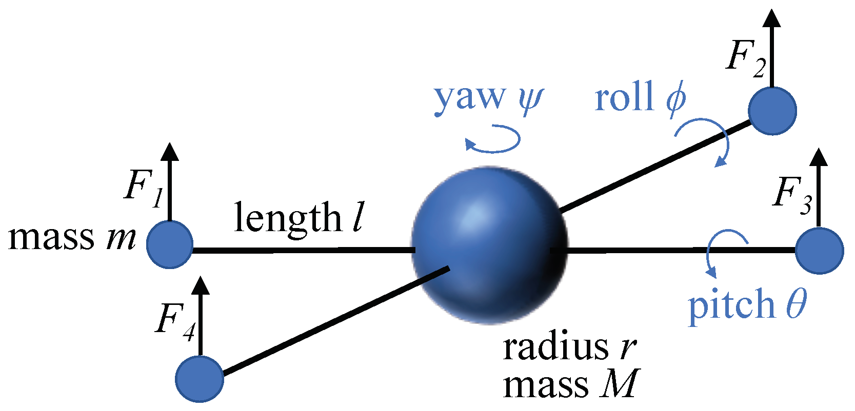
The update mechanism should reflect the way in which the drones approach the next destination based on the real-world environment (i.e., the dynamic model). To establish the dynamic model, first, the kinematic model of a drone is necessary, as shown in Figure 1.

From this kinematic model, the rotation matrix R for mapping the vector from the body frame to the inertial frame can be derived as

$$R=\left[\begin{array}{ccc}{c}_{\varphi }{c}_{\psi }-c_{\theta }{s}_{\varphi }{s}_{\psi }& -c_{\psi }{s}_{\varphi }-c_{\varphi }{c}_{\theta }{s}_{\psi }& s_{\theta }{s}_{\psi }\\ c_{\theta }{c}_{\psi }{s}_{\varphi }+c_{\varphi }{s}_{\psi }& c_{\varphi }{c}_{\theta }{c}_{\psi }-s_{\varphi }{s}_{\psi }& -c_{\psi }{s}_{\theta }\\ s_{\varphi }{s}_{\theta }& c_{\varphi }{s}_{\theta }& c_{\theta }\end{array}\right],$$

(4)

where $c_{\varphi }$ and $s_{\varphi }$ represent $cos\left(\varphi \right)$ and $sin\left(\varphi \right)$, respectively. Then, from Newton’s equation, the linear motion can be derived as

$$m\ddot{x}=\left[\begin{array}{c}0\\ 0\\ -mg\end{array}\right]+R{T}_B+F_D,$$

(5)

where x is the position of the drone, g is the acceleration due to gravity, $F_D$ is the drag force, and $T_B$ is the thrust vector in the body frame. For simplicity, in this paper, the drag force is regarded as 0, and $T_B$ is calculated based on [21]. Additionally, from Euler’s equation, the angular motion can be derived as

$$I\dot{w}=\tau -w\times \left(Iw\right),$$

(6)

where w is the angular velocity vector, I is the inertia matrix, and $\tau$ is a vector of external torques. In this paper, I and $\tau$ are calculated based on [22,23]. Finally, based on these motion equations, the final state space equations for the dynamic model can be derived as

$$\begin{array}{c}\hfill \begin{array}{cc}\hfill \dot{x_1}& =x_2,\hfill \\ \hfill \dot{x_2}& =\left[\begin{array}{c}0\\ 0\\ -g\end{array}\right]+\frac{R{T}_B}{m}+\frac{F_D}{m},\hfill \\ \hfill \dot{x_3}& ={\left[\begin{array}{ccc}1& 0& -s_{\theta }\\ 0& c_{\varphi }& c_{\theta }{s}_{\varphi }\\ 0& -s_{\varphi }& c_{\theta }{c}_{\varphi }\end{array}\right]}^{-1}·x_4,\hfill \\ \hfill \dot{x_4}& =I^{-1}·[\tau -x_3\times \left(I{x}_3\right)],\hfill \end{array}\end{array}$$

(7)

where $x_1$ is the velocity vector, $x_2$ is the acceleration vector, $x_3$ is the angular velocity vector, and $x_4$ is the angular acceleration vector. The model parameters used in this paper are listed in

Table 1. Model parameters.

	Parameters	Values
Environment	Gravity acceleration g	$9.81$
	Draft coefficient b	$0.02$
Kinematic model	M	1.2
	m	0.1
	l	0.3
	r	0.1
Controller	Linear proportional (P) gain	$[300,300,7000]$
	Linear integral (I) gain	$[0.04,0.04,4.50]$
	Linear derivative (D) gain	$[450,450,5000]$
	Angular P gain	$[\mathrm{22,000},\mathrm{22,000},1500]$
	Angular I gain	$[0.00,0.00,1.20]$
	Angular D gain	$[\mathrm{12,000},\mathrm{12,000},0.00]$

.

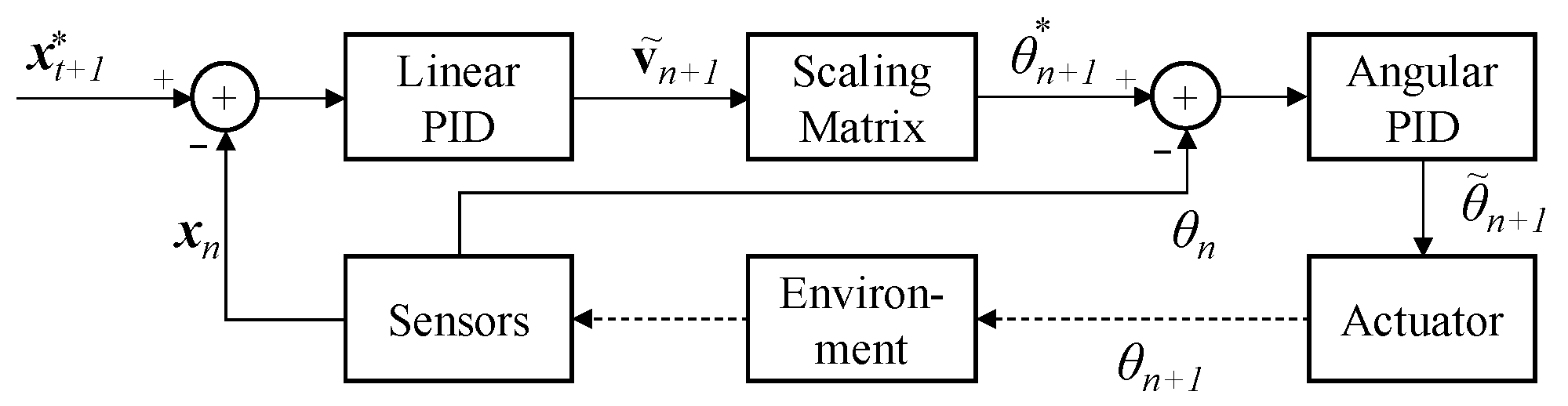
As shown in Figure 2, the control system of the drone can be designed based on a well-known proportional-integral-derivative (PID) control scheme [24]. Note that the control system is not for the low-level motor actuation control, but for the high-level control of the commands transmitted to each drone. In addition, in simulation, the sensor system and the environment can be replaced by the dynamic model derived above.

First, the position error at the n-th control period is calculated. Then, the linear PID system yields the desired displacement ${\tilde{\mathbf{v}}}_{n+1}$, and the next destination posture ${\theta }_{n+1}^{*}$ can be calculated by multiplying a scaling matrix, since it is assumed that the drone is in a piecewise hovering state. Lastly, the angular PID system yields the posture displacement vector ${\tilde{\theta }}_{n+1}$, and the actuation system executes the corresponding throttle commands for the motors. As a result, the drone can gradually approach the next destination ${\mathbf{x}}_{t+1}^{*}$.

Algorithm 1 Swarm search.

$\mathbb{S}$: The search space of the problem $\mathbf{S}$: The swarm of the drones $N_D$: The number of drones in $\mathbf{S}$ $d^k$: The k-th drone ${\mathbf{x}}_t^k$: The position of $d^k$ at iteration t ${\mathbf{v}}_t^k$: The displacement of $d^k$ at iteration t $f\left({\mathbf{x}}_t^k\right)$: The objective function value of ${\mathbf{x}}_t^k$ ${}^g{\mathbf{x}}_t$: The global best position of $\mathbf{S}$ at iteration t ${}^p{\mathbf{x}}_t^k$: The personal best position of $d^k$ at iteration t ${\mathbf{x}}_{t,n}^k$: The position of $d^k$ in the n-th control period at iteration t $\mathbf{c}$: The command output of the controller   (1) Initialize $\mathbf{S}$. for$k=1,2,\dots ,N_D$do     ${\mathbf{x}}_0^k=\mathrm{random}\mathrm{vector}\in \mathbb{S}$     ${\mathbf{v}}_0^k=\mathbf{0}$     Evaluate $f\left({\mathbf{x}}_0^k\right)$     ${}^p{\mathbf{x}}_0^k$ = ${\mathbf{x}}_0^k$     Deploy $d^k$ at ${\mathbf{x}}_0^k$     if $f\left({}^p{\mathbf{x}}_0^k\right)$ is better than $f\left({}^g{\mathbf{x}}_0\right)$ then         ${}^g{\mathbf{x}}_0={}^p{\mathbf{x}}_0^k$     end if end for $t=0$   (2) Update $\mathbf{S}$. for$k=1,2,\dots ,N_D$do     ${\mathbf{v}}_{t+1}^k=w·{\mathbf{v}}_t^k+c·[{\varphi }_1({}^p{\mathbf{x}}_t^k-{\mathbf{x}}_t^k)+{\varphi }_2({}^g{\mathbf{x}}_t-{\mathbf{x}}_t^k)]$     ${\mathbf{x}}_{t+1}^{*k}={\mathbf{x}}_t^k+{\mathbf{v}}_{t+1}^k$     ${\mathbf{x}}_{t,0}^k={\mathbf{x}}_t^k$     $n=0$     while ${\mathbf{x}}_{t,n}^k\ne {\mathbf{x}}_{t+1}^{*k}\mathbf{or}\mathrm{a}\mathrm{collision}\mathrm{is}\mathrm{not}\mathrm{predicted}$ do         c = Controller(${\mathbf{x}}_{t,n}^k,{\mathbf{x}}_{t+1}^{*k}$)         Actuate $d^k$ with c         ($n=n+1$)         Evaluate $\mathbf{f}\left({\mathbf{x}}_{t,n}^k\right)$         if $f\left({\mathbf{x}}_{t,n}^k\right)$ is better than $f\left({}^p{\mathbf{x}}_t^k\right)$ then            ${}^p{\mathbf{x}}_t^k={\mathbf{x}}_{t,n}^k$         end if     end while     if $f\left({}^p{\mathbf{x}}_t^k\right)$ is better than $f\left({}^g{\mathbf{x}}_t\right)$ then         ${}^g{\mathbf{x}}_t={}^p{\mathbf{x}}_t^k$     end if end for ($t=t+1$)   (3) Repeat (2) until a termination condition is met.

2.2. The Overall Procedure of the Swarm Search

The overall procedure of the proposed swarm search is summarized in Algorithm 1, and each step of the algorithm is explained in the following.

First, the swarm of the drones is initialized. For each drone in the swarm, the position is randomly initialized in the search space $\mathbb{S}$, and the displacement is initially set to a zero vector. The objective functions are initially calculated for each drone, and the initial personal best position of each drone ${}^p{\mathbf{x}}_0^k$ is set as the position of itself. Additionally, the initial global best position of the swarm ${}^g{\mathbf{x}}_0$ is set as ${}^p{\mathbf{x}}_0^1$.

Following this, the swarm of the drones is updated. For each drone in the swarm, the position is updated through the drone position update mechanism, as explained above. During the update process, the personal best positions and the global best position are also updated, and this update process is repeated until a termination condition is met. For example, a termination condition can be defined as a maximum number of iterations.

3. Experiment

In the experiment, first, the proposed swarm search method and, as a comparison, the conventional grid search method were implemented. Then, for each test problem, the objective function was designed and applied to both methods. Lastly, 100 simulations were run for each problem and method. Note that in the conventional method, it was assumed that the drones maintained a parallel formation and scanned every location of the search space unidirectionally along the axis in the order of x-, y-, and then z-axes. In addition, in the conventional method, since its position update process is independent of the objective function of the problem, the drones began the search mission at one corner of the search space and the goal was randomly set at each trial. To balance the different conditions of the two methods, in the comparison, one iteration for a drone was defined as one change of the searching direction instead of one visit to a point. Thus, for example, visiting all the grid points from $(-50,0,0)$ to $(50,0,0)$ along the x-axis direction was regarded as one iteration in the conventional method.

In this section, the detailed information about the environment settings is demonstrated, and then the experimental results and their analysis are provided.

3.1. Environment Settings

The proposed method was implemented as a software written in Python (Python software foundation, version 3.5.2) language with Numpy and Matplotlib libraries. The software was run on Linux OS (version 16.04) with Intel i7-6900K CPU, 128 GB DDR4 RAM, and NVIDIA Titan X Pascal GPU. The source code of the simulation engine was based on [25]. The update period of the drone dynamics was set to $0.01$ s and the control period was set to $0.015$ s.

The search mission based on the Rosenbrock function was adopted as Test Problem 1. In this problem, the drones obtained the sensor data at their positions virtually according to the mathematical model which was based on the Rosenbrock function, and the final goal was the position at which the function value was globally minimum. The Rosenbrock function is a well-known benchmark function for numerical optimization because it is hard to find the global minimum in its search space [26,27]. The following is the equation of the sensor data model:

$$\begin{array}{c}\hfill f\left(\mathbf{x}\right)=\sum _{i=1}^{N-1}[100{(\frac{x_{i+1}}{25}-\frac{{x_i}^2}{{25}^2})}^2+{(1-\frac{x_i}{25})}^2],\end{array}$$

(8)

where $\mathbf{x}=[x_1,\dots ,x_N]\in [-50.00,50.00)$. In this problem, N was set to 3 since the real world is three-dimensional, and the number of drones was set to 25. The corresponding global minimum could be found at the position of ($25.00,25.00,25.00$).

For Test Problem 2, an air pollutant search problem was employed. The mission of this problem was to find the origin of the air pollutant at which the pollution concentration was globally maximum. The air pollutant search problem was designed by modeling atmospheric dispersion through a Gaussian air pollutant dispersion equation [28,29]. Figure 3 shows the visualization of the Gaussian air pollutant dispersion on x- and z-axes, which was originally from [30].

The Gaussian air pollutant dispersion equation can be written as:

$$\left\{\begin{array}{c}\begin{array}{cc}\hfill C(x,y,z)& =\frac{Q}{u}·\frac{f}{{\sigma }_y\left(x\right)\sqrt{2\pi }}·\frac{g_1+g_2}{{\sigma }_z\left(x\right)\sqrt{2\pi }}\hfill \\ & =\frac{Q}{2\pi ·{\sigma }_y\left(x\right)·{\sigma }_z\left(x\right)·u}·e^{-\frac{y^2}{2{\sigma }_y{\left(x\right)}^2}}·[e^{-\frac{{(z-H)}^2}{2{\sigma }_z{\left(x\right)}^2}}+e^{-\frac{{(z+H)}^2}{2{\sigma }_z{\left(x\right)}^2}}],\mathrm{if}x\ge 0,\hfill \end{array}\hfill \\ C(x,y,z)=0,\hspace{1em}\hspace{1em}\hspace{1em}\hspace{1em}\hspace{1em}\hspace{1em}\hspace{1em}\hspace{1em}\hspace{1em}\hspace{1em}\hspace{1em}\hspace{1em}\hspace{1em}\hspace{1em}\hspace{1em}\hspace{1em}\hspace{1em}\hspace{1em}\hspace{1em}\hspace{1em}\hspace{1em}\hspace{1em}\hspace{1em}\hspace{1em}\mathrm{otherwise},\hfill \end{array}\right.$$

(9)

where:

$$\begin{array}{c}\hfill \begin{array}{cc}\hfill x,y& \in [-50.00,50.00),z\in [0.00,50.00)\hfill \\ \hfill f& =\mathrm{crosswind}\mathrm{dispersion}=e^{-\frac{y^2}{2{\sigma }_y^2}}\hfill \\ \hfill g_1& =\mathrm{vertical}\mathrm{dispersion}\mathrm{with}\mathrm{no}\mathrm{reflections}=e^{-\frac{{(z-H)}^2}{2{\sigma }_z^2}}\hfill \\ \hfill g_2& =\mathrm{vertical}\mathrm{dispersion}\mathrm{for}\mathrm{reflection}\mathrm{from}\mathrm{the}\mathrm{ground}=e^{-\frac{{(z+H)}^2}{2{\sigma }_z^2}}\hfill \\ \hfill C& =\mathrm{concentration}\mathrm{of}\mathrm{emissions},\mathrm{in}\mathrm{g}/\mathrm{m}{}^3\hfill \\ \hfill Q& =\mathrm{source}\mathrm{pollutant}\mathrm{emission}\mathrm{rate},\mathrm{in}\mathrm{g}/\mathrm{s}\hfill \\ \hfill u& =\mathrm{horizontal}\mathrm{wind}\mathrm{velocity}\mathrm{along}\mathrm{the}\mathrm{plume}\mathrm{centerline},\mathrm{in}\mathrm{m}/\mathrm{s}\hfill \\ \hfill H& =\mathrm{height}\mathrm{of}\mathrm{emission}\mathrm{plume}\mathrm{centerline}\mathrm{above}\mathrm{ground}\mathrm{level},\mathrm{in}\mathrm{m}\hfill \\ \hfill {\sigma }_z& =\mathrm{vertical}\mathrm{standard}\mathrm{deviation}\mathrm{of}\mathrm{the}\mathrm{emission}\mathrm{distribution},\mathrm{in}\mathrm{m}\hfill \\ \hfill {\sigma }_y& =\mathrm{horizontal}\mathrm{standard}\mathrm{deviation}\mathrm{of}\mathrm{the}\mathrm{emission}\mathrm{distribution},\mathrm{in}\mathrm{m}.\hfill \end{array}\end{array}$$

From [29], ${\sigma }_y\left(x\right)$ and ${\sigma }_z\left(x\right)$ can be determined as:

$$\begin{array}{c}\hfill \begin{array}{cc}\hfill {\sigma }_y\left(x\right)& =e^{[I_y+J_y·log(x+ϵ)+K_y·log{(x+ϵ)}^2]},\hfill \\ \hfill {\sigma }_z\left(x\right)& =e^{[I_z+J_z·log(x+ϵ)+K_z·log{(x+ϵ)}^2]},\hfill \end{array}\end{array}$$

(10)

where $ϵ$ was set to ${10}^{-10}$ in this problem.

In this problem, the number of drones was set to 15. In addition, Q, u, and H were set to 10, 3, and 10, respectively. It was assumed that the atmosphere was in a neutral state, and, according to the classification of stability class proposed in [31,32], $I_y$, $J_y$, $K_y$, $I_z$, $J_z$, and $K_z$ were set to $-2.55$, $1.04$, $-0.01$, $-3.19$, $1.11$, and $-0.03$, respectively. Based on these settings, the corresponding global maximum could be found at the position of ($0.00,0.00,10.00$).

3.2. Experimental Results

The results demonstrate the effectiveness of the proposed method through the following figures describing the trajectories of the drones with the proposed method, as well as the tables representing the statistical comparisons between the proposed and conventional methods.

Figure 4 shows the simulation of Test Problem 1 through the proposed method at iterations 1, 10, 50, and 1500. As shown in the figure, the drones successfully found the target position at which the Rosenbrock function had the minimum value within 150 iterations. Note that the drones were unaware of the function as well as its derivatives.

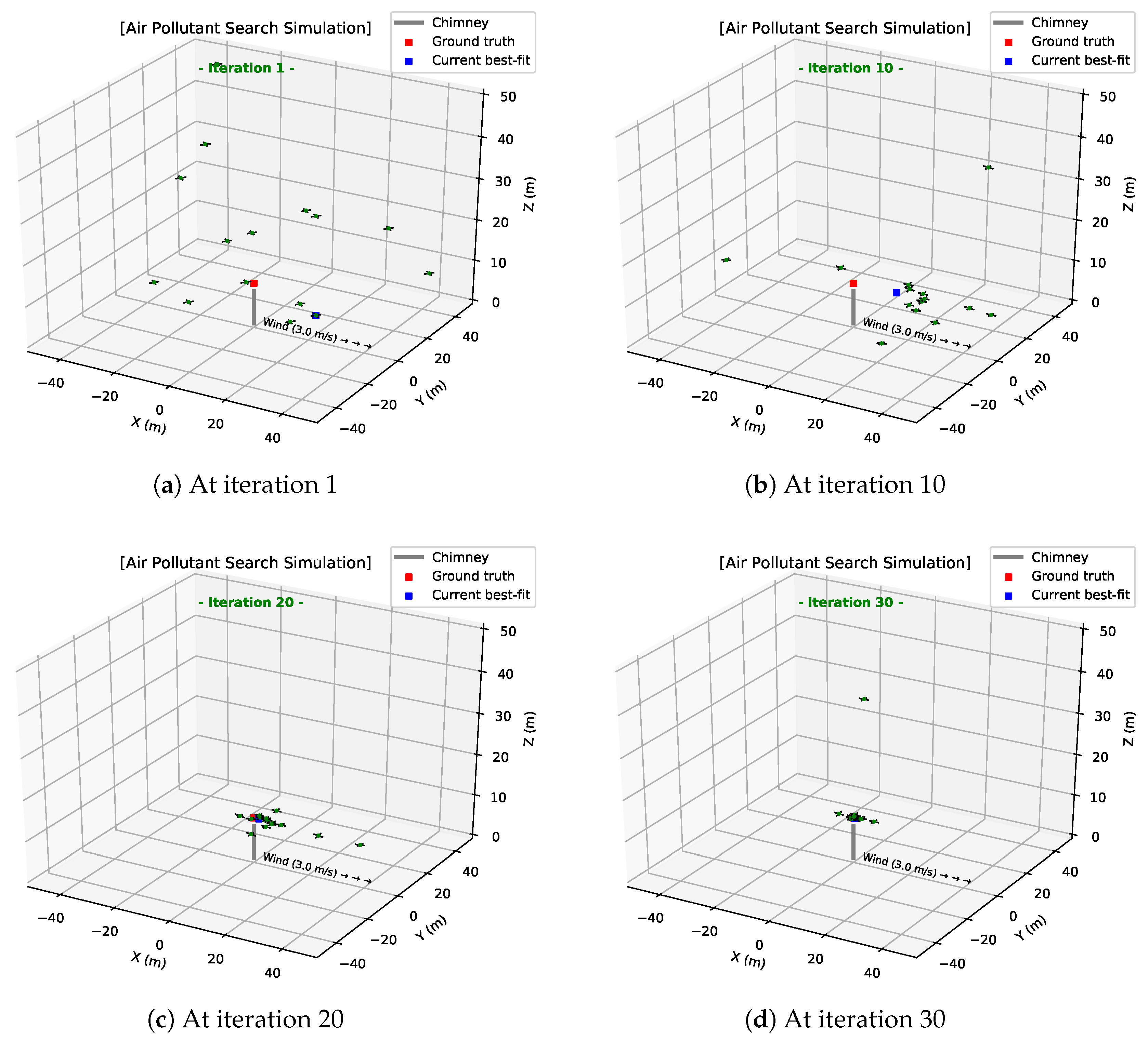
Figure 5 shows the simulation of Test Problem 2 through the proposed method at iterations 1, 10, 20, and 30. As shown in the figure, the drones successfully found the target position at which the pollutant was being emitting within 30 iterations. Note that the drones had no knowledge of the dispersion model, and could simply measure the air pollution concentrations at their positions.

The full simulation videos for Test Problems 1 and 2 are provided through the YouTube links “https://youtu.be/fIUmsO5B4CA” and “https://youtu.be/cdlCZQeN-Bo”, respectively. The videos show that the drones could find the global minimum or maximum under non-convex or near non-convex environments. The videos also show that the drones could be controlled stably in real-time, and the dynamic model was well-applied considering the real-world environment.

Moreover,

Table 2. The averages ($AVG$s) and standard deviations ($STD$s) of the number of iterations n for the methods to satisfy the termination condition ($\mathit{TC}$).

Problem	Proposed		Conventional		$\mathit{TC}$
	$\mathit{AVG}\left(\mathit{n}\right)$	$\mathit{STD}\left(\mathit{n}\right)$	$\mathit{AVG}\left(\mathit{n}\right)$	$\mathit{STD}\left(\mathit{n}\right)$
1	141.72	37.73	409.68	244.95	$d_{err}<2.0$
2	27.41	7.62	366.66	211.01	$d_{err}<2.0$

shows the averages ($AVG$s) and standard deviations ($STD$s) of the number of iterations n for the proposed and conventional methods to satisfy the corresponding termination condition ($TC$) about error distance $d_{err}$. Since the search space was based on a real-world environment, the unit of distance was meters. If we consider the size of commonly-used drones (approximately 1.0 m), the minimum grid size for the conventional grid search should be greater than 1.0 m. Based on this condition, we can approve that the drone is close enough to the goal if $d_{err}$ is less than 2.0, which is double the minimum grid size. Additionally, the $AVG$s and $STD$s of the final $d_{err}$ for the proposed and conventional methods with the limited number of iterations $n_{limit}$ are shown in

Table 3. The $AVGs$ and $STDs$ of the error distance ($d_{err}$) for the methods with the limited number of iterations ($n_{limit}$).

Problem	Proposed		Conventional		${\mathit{n}}_{\mathit{limit}}$
	$\mathit{AVG}\left({\mathit{d}}_{\mathit{err}}\right)$	$\mathit{STD}\left({\mathit{d}}_{\mathit{err}}\right)$	$\mathit{AVG}\left({\mathit{d}}_{\mathit{err}}\right)$	$\mathit{STD}\left({\mathit{d}}_{\mathit{err}}\right)$
1	0.88	0.56	58.79	51.82	200
2	0.04	0.05	64.14	39.10	50

. Smaller values of both n and $d_{err}$ are desirable, where n and $d_{err}$ imply the speed and the accuracy of the methods, respectively. As displayed in the tables, the proposed method could find the target more quickly and more accurately and robustly than the conventional method. Note that the proposed method showed a more powerful result in the real-world problem (e.g., Test Problem 2) than the virtual problem (e.g., Test Problem 1).

4. Conclusions

In this paper, a novel search method for a swarm of quadcopter drones was proposed. In the proposed method, inspired by the phenomena of swarms in nature, drones could effectively look for better locations by investigating the evidence from the surroundings and communicating with each other. The position update mechanism was implemented based on the particle swarm optimization algorithm (a well-known swarm-based optimization algorithm), as well as the dynamic model of the drones, which was used to take the real-world environment into account. In addition, the mechanism could be processed in real-time along with the movements of the drones. The experimental results showed that through the proposed method, the drones could find the target more quickly and accurately than by the conventional algorithm. Most importantly, the proposed method has high practical potential, considering that the drones were simulated in real-time and the dynamic model sufficiently reflected the real-world environment.

References

- Cacace, J.; Finzi, A.; Lippiello, V.; Loianno, G.; Sanzone, D. Aerial service vehicles for industrial inspection: task decomposition and plan execution. Appl. Intell. 2015, 42, 49–62. [Google Scholar] [CrossRef]
- Lippiello, V.; Siciliano, B. Wall inspection control of a VTOL unmanned aerial vehicle based on a stereo optical flow. In Proceedings of the IEEE/RSJ International Conference on Intelligent Robots and Systems (IROS), Vilamoura, Portugal, 7–12 October 2012; pp. 4296–4302. [Google Scholar]
- Bevacqua, G.; Cacace, J.; Finzi, A.; Lippiello, V. Mixed-Initiative Planning and Execution for Multiple Drones in Search and Rescue Missions. In Proceedings of the Twenty-Fifth International Conference on Automated Planning and Scheduling, ICAPS, Jerusalem, Israel, 7–11 June 2015; pp. 315–323. [Google Scholar]
- Cacace, J.; Finzi, A.; Lippiello, V.; Furci, M.; Mimmo, N.; Marconi, L. A control architecture for multiple drones operated via multimodal interaction in search & rescue mission. In Proceedings of the IEEE International Symposium on Safety, Security, and Rescue Robotics (SSRR), Lausanne, Switzerland, 23–27 October 2016; pp. 233–239. [Google Scholar]
- Cacace, J.; Finzi, A.; Lippiello, V. Multimodal interaction with multiple co-located drones in search and rescue missions. arXiv, 2016; arXiv:1605.07316. [Google Scholar]
- Cui, J.Q.; Phang, S.K.; Ang, K.Z.; Wang, F.; Dong, X.; Ke, Y.; Lai, S.; Li, K.; Li, X.; Lin, F.; et al. Drones for cooperative search and rescue in post-disaster situation. In Proceedings of the IEEE 7th International Conference on Cybernetics and Intelligent Systems (CIS) and IEEE Conference on Robotics, Automation and Mechatronics (RAM), Angkor Wat, Cambodia, 15–17 July 2015; pp. 167–174. [Google Scholar]
- Rivera, A.; Villalobos, A.; Monje, J.; Mariñas, J.; Oppus, C. Post-disaster rescue facility: Human detection and geolocation using aerial drones. In Proceedings of the IEEE Region 10 Conference (TENCON), Singapore, 22–25 November 2016; pp. 384–386. [Google Scholar]
- Cui, J.Q.; Phang, S.K.; Ang, K.Z.; Wang, F.; Dong, X.; Ke, Y.; Lai, S.; Li, K.; Li, X.; Lin, J.; et al. Search and rescue using multiple drones in post-disaster situation. Unmanned Syst. 2016, 4, 83–96. [Google Scholar] [CrossRef]
- Bekhti, M.; Achir, N.; Boussetta, K. Swarm of Networked Drones for Video Detection of Intrusions. In Proceedings of the International Wireless Internet Conference, Tianjin, China, 16–17 December 2017; pp. 221–231. [Google Scholar]
- Šulák, V.; Kotuliak, I.; Čičák, P. Search using a swarm of unmanned aerial vehicles. In Proceedings of the 15th International Conference on Emerging eLearning Technologies and Applications (ICETA), Stary Smokovec, Slovakia, 26–27 October 2017; pp. 1–6. [Google Scholar]
- Gaynor, P.; Coore, D. Towards distributed wilderness search using a reliable distributed storage device built from a swarm of miniature UAVs. In Proceedings of the IEEE International Conference on Unmanned Aircraft Systems (ICUAS), Orlando, FL, USA, 27–30 May 2014; pp. 596–601. [Google Scholar]
- Altshuler, Y.; Pentland, A.; Bruckstein, A.M. Swarms and Network Intelligence in Search; Springer: Berlin, Germany, 2018. [Google Scholar]
- Leavitt, H.J. Some effects of certain communication patterns on group performance. J. Abnorm. Soc. Psychol. 1951, 46, 38. [Google Scholar] [CrossRef]
- Bandura, A. Social Foundations of Thought and Action: A Social Cognitive Theory; Prentice-Hall, Inc.: Englewood Cliffs, NJ, USA, 1986. [Google Scholar]
- Kennedy, J. The particle swarm: social adaptation of knowledge. In Proceedings of the IEEE International Congress on Evolutionary Computation, Indianapolis, IN, USA, 13–16 April 1997; pp. 303–308. [Google Scholar]
- Eberhart, R.C.; Shi, Y.; Kennedy, J. Swarm Intelligence; Elsevier: New York, NY, USA, 2001. [Google Scholar]
- Pugh, J.; Martinoli, A. Inspiring and modeling multi-robot search with particle swarm optimization. In Proceedings of the IEEE Swarm Intelligence Symposium, Honolulu, HI, USA, 1–5 April 2007; pp. 332–339. [Google Scholar]
- Couceiro, M.S.; Rocha, R.P.; Ferreira, N.M. A novel multi-robot exploration approach based on particle swarm optimization algorithms. In Proceedings of the IEEE International Symposium on Safety, Security, and Rescue Robotics (SSRR), Kyoto, Japan, 1–5 November 2011; pp. 327–332. [Google Scholar]
- Kennedy, J. Particle swarm optimization. In Encyclopedia of Machine Learning; Springer: Berlin, Germany, 2011; pp. 760–766. [Google Scholar]
- Du, K.L.; Swamy, M. Particle swarm optimization. In Search and Optimization by Metaheuristics; Springer: Berlin, Germany, 2016; pp. 153–173. [Google Scholar]
- Staples, G. Propeller Static & Dynamic Thrust Calculation. 2013. Available online: https://www.electricrcaircraftguy.com/2013/09/propeller-static-dynamic-thrust-equation.html (accessed on 13 April 2014).
- Beard, R. Quadrotor Dynamics and Control Rev 0.1; All Faculty Publications; Brigham Young University: Provo, UT, USA, 2008. [Google Scholar]
- Khan, M. Quadcopter flight dynamics. Int. J. Sci. Technol. Res. 2014, 3, 130–135. [Google Scholar]
- Praveen, V.; Pillai, S. A Modeling and simulation of quadcopter using PID controller. Int. J. Control Theory Appl. 2016, 9, 7151–7158. [Google Scholar]
- Majumdar, A. Quadcopter Simulator. 2017. Available online: https://github.com/abhijitmajumdar/Quadcopter_simulatorl (accessed on 19 February 2018).
- Rosenbrock, H. An automatic method for finding the greatest or least value of a function. Comput. J. 1960, 3, 175–184. [Google Scholar] [CrossRef]
- Shi, Y.; Eberhart, R.C. Empirical study of particle swarm optimization. In Proceedings of the IEEE International Congress on Evolutionary Computation, Washington, DC, USA, 6–9 July 1999; Volume 3, pp. 1945–1950. [Google Scholar]
- Juan, S.; Jiong, S.; Bao, Q.; Yusen, D.; Qiang, W. An Industrid air pollution dispersion system based on Gauss dispersion model. Environ. Pollut. Control 2005, 7, 11. [Google Scholar]
- Seinfeld, J.H.; Pandis, S.N. Atmospheric Chemistry and Physics: From Air Pollution to Climate Change; John Wiley & Sons: Hoboken, NJ, USA, 2016. [Google Scholar]
- Abdel-Rahman, A.A. On the atmospheric dispersion and Gaussian plume model. In Proceedings of the 2nd International Conference on Waste Management, Water Pollution, Air Pollution, Indoor Climate, Corfu, Greece, 26–28 October 2008; pp. 31–39. [Google Scholar]
- Pasquill, F. Atmospheric dispersion of pollution. Q. J. R. Meteorol. Soc. 1971, 97, 369–395. [Google Scholar] [CrossRef]
- Hanna, S.R.; Briggs, G.A.; Hosker, R.P., Jr. Handbook on Atmospheric Diffusion; Technical Report; National Oceanic and Atmospheric Administration: Oak Ridge, TN, USA; Atmospheric Turbulence and Diffusion Lab.: Oak Ridge, TN, USA, 1982.
Figure 1.
The physical model of a quadcopter drone.
Figure 2.
The control system of a quadcopter drone.
Figure 3.
The visualization of the Gaussian air pollutant dispersion on x- and z-axes.
Figure 4.
Screenshots of the simulation of Test Problem 1 by the proposed method.
Figure 5.
Screenshots of the simulation of Test Problem 2 by the proposed method.