Optimize Rotating Wind Energy Rotor Blades Using the Adjoint Approach


1
ForWind, University of Oldenburg, Ammerländer Heerstr. 114-118, 26129 Oldenburg, Germany
2
Fraunhofer IWES, Küpkersweg 70, 26129 Oldenburg, Germany
*
Author to whom correspondence should be addressed.
Appl. Sci. 2018, 8(7), 1112; https://doi.org/10.3390/app8071112
Submission received: 5 June 2018
/
Revised: 2 July 2018
/
Accepted: 6 July 2018
/
Published: 10 July 2018
(This article belongs to the Special Issue Wind Turbine Aerodynamics)
Abstract
:Wind energy rotor blades are highly complex structures, both combining a large aerodynamic efficiency and a robust structure for lifetimes up to 25 years and more. Current research deals with smart rotor blades, improved for turbulent wind fields, less maintenance and low wind sites. In this work, an optimization tool for rotor blades using bend-twist-coupling is developed and tested. The adjoint approach allows computation of gradients based on the flow field at comparably low cost. A suitable projection method from the large design space of one gradient per numerical grid cell to a suitable design space for rotor blades is derived. The adjoint solver in OpenFOAM is extended for external flow. As novelty, we included rotation via the multiple reference frame method, both for the flow and the adjoint field. This optimization tool is tested for the NREL Phase VI turbine, optimizing the thrust by twisting of various outer parts between 20–50% of the blade length.
1. Introduction
The generated electric power from wind turbines increases linearly with the swept rotor area. Therefore, wind turbines grow larger and larger. Otherwise, limits in maximal mountable rotor weight and constraints coming from material science restrict the growth of rotor blades. Further limiting factors are alternating wind loads, gusts, turbulences and rotational forces. As wind turbines are normally designed for a life time of 20–25 years, the estimated total amount of rotations is about , which leads to – load changes. Periodic loads due to the vertical wind velocity gradient and the tower shadow, each one of them proportional to the blade rotation frequency, add up to this [1]. Added to those load changes due to the rotational movement are the wind loads, which were shown to be highly intermittent [2]. At the same time, most favorable sites for wind turbines with little turbulence intensity and large average wind speeds are already exploited, such that either repowering or worse sites are chosen in order to increase the generated wind power [3]. For slow average wind speeds, slender blades are favorable, which react even on small wind velocities due to a large aerodynamic efficiency. This enforces the trend towards long, slender blades. Such blades are prone to elastic deformations and even more influenced by wind load changes.
In return, this might lead to critical fatigue of the material, both from blades, but also from bearings and support structures. However, flexibility and light structures offer the possibility of passive control. The pitch systems of wind turbine blades are too slow to react on highly intermittent load fluctuations within the wind field, the use of structural bend twist coupling, which reacts instantly on aerodynamic loads, is a promising concept to reduce the amount of load changes and therefore of fatigue by a pre-designed deformation of the blade [4]. Especially adaptive changes in the twist of the blade can reduce the angle of attack and thus lead to a significant load reduction, which results in a longer life time or less cumbersome maintenance of the wind turbine blades and therefore in the end in lower specific costs of energy [5,6].
Based on the actual development in rotor design, we present in this work an optimization tool for the aerodynamics of rotating rotor blades within the open-source toolbox for numerical simulations OpenFOAM. This tool is tested for the optimization of the twist distribution in order to reduce the overall thrust force. Gradient-based optimization offers on the one hand the large advantage of a high-quality search direction for optima. On the other hand, only local optima are found. Thus, this method is suitable if there is not more than one optimum or if the initial point is not too far away from the global optimum. In our case, the aerodynamics of wind turbine rotor blades can be considered as sophisticated, so that the mentioned disadvantage of the gradient-based method can be neglected, while the advantage of a high-quality search direction is utilized. The continuous adjoint approach is used for the computation of gradients. In contrast to other methods, the adjoint approach is marked by the independence of the computational cost on the amount of design parameters, thus no full simulation per each single design parameter is required [7]. This qualifies the adjoint approach for the combination with computationally expensive Computational Fluid Dynamics (CFD). The optimization is based on the solution of steady-state flow equations of the current blade geometry. Obtained gradients are then evaluated to find the optimum. The implementation of the continuous adjoint equations in OpenFOAM was firstly done by Ohtmer [8] for ducted flows. Several publications show the applicability of the adjoint approach in combination with CFD, both for external and ducted flows [9,10,11,12]. However, these works showed the application either for low Reynolds numbers, for non-rotating fields or using porosity of numerical cells to impact the shape of ducts. Thus, the usage of the adjoint approach in wind energy needed further development and investigation. The adjoint solver for ducted flows could be used in the field of diffuser-augmented wind turbines. The generalized actuator disc theory, proposed by Jamieson [13] and extended by Lui and Yoshida [14], could be used within OpenFOAM to compute optimal difuser geometries with maximal effective diffuser efficiency. In this work, we focus on the optimization of rotor blade geometries of wind turbines in open flow. Therefore, the adjoint equations in OpenFOAM were adopted for external flow and the resulting gradients were verified against finite differences by Schramm [15,16]. It was shown in Schramm [16] that the adjoint approach can be used in wind energy relevant cases, in that work shown for the optimization of an airfoil slat. In a previous work, the adjoint optimization in OpenFOAM has been tested against other optimization strategies, like finite differences and Nelder-Mead. The independence from the amount of design parameters was shown there, as well as the applicability for wind energy relevant profiles [17].
In this work, the adjoint approach is used for rotating geometries and large Reynolds numbers. To the authors’ knowledge, this combination poses a novelty and offers new areas of application. It should be noted that the rotational flow around rotor blades is complex and it is generally already challenging to achieve low residuals for such flows using stationary flow solvers. In addition, the NREL Phase VI turbine is stall regulated and the chosen velocity already corresponds to the rated velocity. Thus, the flow is separated at the inner blade region, leading to poor convergence behavior of the flow field. The adjoint field is driven by the flow field so that the errors in the flow field transfer directly to the adjoint field and decrease the convergence quality of it. This challenging set-up is used purposely to thoroughly test the optimization tool, its convergence and applicability.
The paper is structured as follows. First, the theory of the underlying optimization is given, including the gradient estimation via the adjoint approach and their processing is explained in Section 2. In Section 3, the simulation set-up in OpenFOAM is shown, as well as the optimization set-up and cases. Finally, results of the optimization are given in Section 4 followed by a conclusion in Section 5.
2. Optimization Method
To design a blade using bend-twist-coupling as a passive control mechanism, a favorable deformed blade shape that ensures the optimal load reductions has to be determined. The deformed blade shape can then be integrated into the structural blade design where layer lay-up or geometrical sweep are options to achieve the favorable deformations. To find those favorable deformations, an optimization tool for the aerodynamic shape of the rotor blades based on the continuous adjoint approach is implemented in OpenFOAM. The gradients are then projected to central nodes, adopting geometry updates like in Fluid–Structure Interaction (FSI) based on a beam. In this work, the optimization is directly coupled with the CFD toolbox, allowing direct communication and data usage. This tool is used to find deformations that reduce loads under certain load conditions. Our approach is that the general geometrical shape of the 2D profiles is constant, and only elastic deformations are allowed, such as changing the twist angle along the blade. In order to test the optimization tool and its performance, the optimizations are conducted for the same blade under the same inflow conditions but with a variable movable part of the blade and different aimed values. Therefore, between and of the outer blade are allowed to be changed with respect to its twist distribution. This investigation allows an assessment of the effect of complex lay-up within large to short parts of the blades, respectively. The optimization in this work is based on the reduction of the thrust that effects the blade root bending, tower bending and other forces. Although no constraints were used, it is possible to include limiting ranges for other forces in further applications of this tool.
In addition, the developed optimization tool allows other definitions of design parameters and cost functions.
Details regarding the adjoint approach are discussed next.
2.1. Gradient Estimation by the Adjoint Approach
The adjoint approach allows for computing the gradient of a cost function with respect to the design parameters independently from the amount of design parameters. The main idea is to build a Lagrangian function, which includes both the cost function to be optimized and the constraint and thus can be used for constrained optimization problems. For optimization based on CFD, the flow equations have to be satisfied in each optimization point. Thus, the constraining functions are the Navier–Stokes equations (NSE)
with u and p being the flow velocity and pressure, respectively. The rate of strain tensor for any given vector x is defined as . This notation is used for the velocity and adjoint velocity in the flow and adjoint field, respectively. The viscosity is a sum of the molecular and turbulent viscosity.
The Lagrangian function
combines the cost function I with the NSE in the flow domain . The Lagrangian multipliers, which allow the combination of the cost function with the NSE, are the adjoint velocity and adjoint pressure .
The adjoint field equations
result from the variation of the Lagrangian function with respect to the flow and design variables. A step-by-step derivation of the adjoint field is shown in the work of Othmer [18].
In this work, the flow equations are solved following the SIMPLE algorithm [19]. The continuous adjoint equations are similar to the ones from the flow field, such that similar numerical solving strategies can be applied. The frozen turbulence approach is applied, meaning that the viscosity from the flow field is also applied for the adjoint field, without additional adjoint turbulence equations [7,20].
In the following, flow gradients refer to changes in the flow field over distance, whereas gradients are the gradients of the cost function w.r.t. the design variables.
The two discussed fields have to be solved once, respectively, to derive all gradients at each numerical grid node on the blade geometry surface. Thus, the additional cost for the gradient information at any amount of design parameters equals the cost of solving a second set of partial differential equations that are derived from the flow field equations. One consequence from this is that the adjoint field is driven by the flow field on which it is based. This can also be seen in Equations (4) and (5) and leads to a transfer of the error made in the flow field computations to the adjoint field. Thus, the adjoint field is less stable. The large advantage of the adjoint method compared to other gradient estimation methods is that the amount of necessary solutions of the flow field doesn’t scale with the amount of design parameters. This is especially desirable when working with gradient based optimization based on fully resolved simulations.
2.2. Gradient Projection and Evaluation
For an optimization procedure, it is an essential point to work out suitable parameters. The definition of the rotor blade’s shape can be done in various ways. It was shown in [17] that the free parametrization, i.e., all numerical grid points are design parameters, is not suitable for optimizing rotor blades. This results from large flow field gradients in the chordwise direction and in the spanwise direction, which transfer to the computed gradient. In areas of large gradients, the deformation is much larger, which leads to bumps and uneven surfaces. Instead of the use of all grid points, one can select parameters that define the blade geometry, like the twist distribution, thickness of airfoils along the blade and so forth, which define the blade geometry. For the developed optimization tool, an automatized routine is implemented that allows the projection of the gradients at each numerical grid cell to a reduced design space.
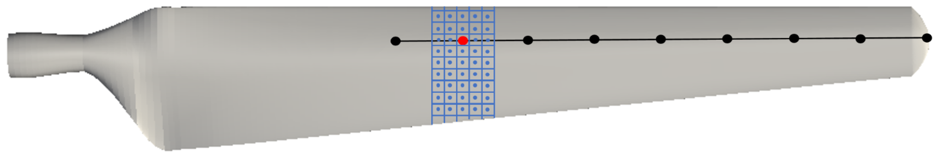
The flow around airfoils and rotor blades is highly sheared with large flow gradients both in velocity and pressure. Therefore, the numerical grid has to be appropriately fine at those areas in order to catch the flow phenomena. Typical values for the amount of cells in the chordwise direction vary between 250 and 350. The adjoint approach leads to gradient information on each of these cells. To use a parametrization with less design parameters, a projection from these 250–350 gradients on less design parameters is implemented. The main idea for the parametrization used in the optimization tool comes from FSI using a finite beam. The gradients are treated like forces acting on the blade and therefore projected on central nodes. The principle of the parametrization is shown in Figure 1.
As a pre-processing step, the blade is split into a selected amount of elements. Each of these elements has a central node, which is represented by a big red dot in Figure 1. All big dots represent one final design parameter each. The amount of design parameters is chosen beforehand by the user. The number can be controlled by adapting a dictionary that is defined for the usage of the developed tool. In this exemplary case, there are nine design parameters. For one exemplary element, the structured grid is shown with thin blue lines. In the figure, the represented grid has been coarsened for the sake of clarity. Within each cell of this grid, the small blue dot represents the local gradient of each grid cell, computed via the adjoint approach. The adjoint gradients are then transferred onto the nodes depending on the distance of the local cell to the central node of the element. Evaluating the projected gradients then leads to a movement of the nodes, which act like beam nodes. The difference to FSI is that the structure is not solved, and it is assumed that any movement given by the gradients can be realized. This assumption is necessary for the presented optimization. The final, optimized geometries can be used within the blade design process as an input to the design of the structure, for example when passive control shall be applied. Therefore, the structure is not final when the optimization takes place. In addition, the movement of the blade due to a structural response might interfere with the movement given by the gradients.
The pre-condition for this projection is that an elastic deformation shall be guaranteed, where the blade cross sections are constant. However, even this parametrization on a reduced design space takes into account the gradient information of each numerical grid cell, as each local gradient is used within the projection. This makes the usage of the adjoint approach convenient.
The gradients of each numerical cell that belongs to one central node of an element are transferred to two vectors. One is acting like a force, that can be compared to the bending force in FSI and one is acting like a torsional moment that can be compared to a moment of force responsible for twisting in FSI. After projection, each element of the blade has these two gradient vectors. In a second step, for each of these two vector types, the maximal value among all elements is used for normalization, respectively. This leads to a similar range of values, with a maximal magnitude of one, for both. With this, weighting factors can be introduced that allow for augmenting one of the movements, when needed. Optional smoothing by neighboring elements is implemented and can be switched on and off via a dictionary. In between the elements, an interpolation is used to avoid kinks on the blade surface. This interpolation as well as the mesh update is taken from an in-house FSI solver by Dose [21].
The projected gradients can then be used within an optimization algorithm for gradient based optimization. The most direct way to use the gradients is via the steepest descent algorithm, which is also used in this work. According to the direction and dimension of the gradient, changes in the geometry are performed for all selected design parameters. Depending on the slope of the design space, the optimal search direction (pointing to the minimum) can differ largely from the gradient direction. In these cases, the steepest descent search results in a highly inefficient, but typical zigzag pattern. Consequently, the method of steepest descent has found little applicability in practice, since its performance is in most cases largely inferior to second-order methods, like the Quasi-Newton method. For high-dimensional design spaces, though, the method of steepest descent can be advantageous, since it does not require the estimation of the inverse Hessian, which scales with the number of design variables [22].
3. Simulation and Optimization Set-Ups
This is a conceptual work in which we want to show a new optimization approach for wind energy applications. Therefore, the optimizations are conducted for the NREL Phase VI turbine. This turbine is a stall-regulated, two-bladed turbine with a rated power of kW. It was used for experiments in the NASA/Ames 24.4 m × 36.6 m wind tunnel [23] and is often used for validation of CFD. The S809 airfoil with thickness was used for the construction of the blade [24]. In this work, the cone angle of the rotor is and the pitch angle of the blade is .
To include rotational effects in steady-state simulations, the Multiple Reference Frame (MRF) is used. The rotation is modelled via a source force, that adds a rotational component to each cell. This way, the rotor does not have to move within the mesh reducing the computational effort, as no mesh update is necessary to include the rotation. The MRF method is also adopted to the adjoint field, so that the used schemes and solution methods for both fields stay similar.
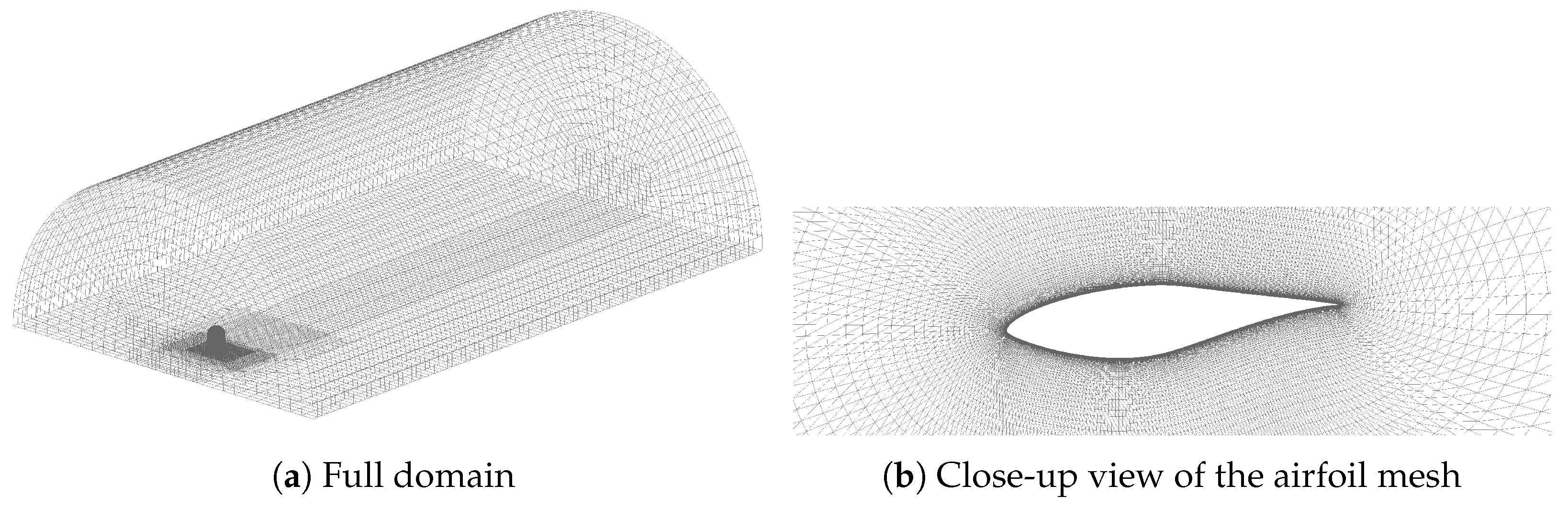
The mesh used in this work was created by the bladeBlockMesher (BBM) developed by Rahimi et al. [25] for the automatic mesh generation for wind turbine rotor blades. The grid quality and validation based on the NREL Phase VI turbine is also shown in their publication. In this work, a grid with 5.2 million cells is used with a -value below 1. A symmetry plane is used to exploit the symmetry of the two bladed rotor. In Figure 2 the domain and the mesh around a cut along the chord of the blade is shown.
A rounded tip is created and meshed via the BBM. The k--SST turbulence model is chosen for the flow field, whereas for the adjoint field the frozen turbulence approach is applied. This approach was used in various publications and it was shown that the gradient quality is adequate [7,18]. Standard boundary conditions are applied, similar to those in Rahimi [25]. The inflow velocity is 10 m/s and the rotational speed is rad/s, i.e., 72 rpm and the density equals kg/m. This velocity leads the stall regulated turbineto already partially separate flow at large parts of the blade. Steady state CFD computations of this turbine at separated flow are known to differ from the experimental data at those separated areas [25]. As it was shown above, the adjoint field is driven by the flow field and therefore it is expected that the adjoint field converges even less as good as the flow field. Still, this velocity was chosen in this work, as even small changes in AoA have a large impact on the forces, when separation is reduced.
As the adjoint field moves upstream, the boundary conditions are switched compared to the flow field. The adjoint velocity has a Neumann boundary condition at the inlet, and a Dirichlet boundary condition at the outlet and at the blade. The adjoint pressure has a Dirichlet boundary condition at the inlet and Neumann boundary condition at the outlet and blade. For a higher stability, the adjoint velocity at the hub is put to zero. This was necessary, as the transition between hub and blade root led to large instabilities in the adjoint field.
It was shown in Section 2.1 that the adjoint field is driven by the primal field. Therefore, preconverged solutions of the flow field are used in order to stabilize the adjoint equations. A convergence of the velocity up to a residual in the range of is aimed before the adjoint field equations are switched on. An initial study using the same numerical grid based on the initial geometry was conducted to find adequate amounts of CFD iterations to reach good convergence of both fields. As a result, 25,000 iterations are used solving the flow field based on the SIMPLE algorithm [19]. An additional 15,000 iterations are used for solving the adjoint and flow field before the optimization tool is started. These pre-converged fields are used for all optimizations, as the initial blade geometry and flow boundary conditions are identical. Starting from the total amount of 40,000 iterations used for pre-convergence of the fields, the optimizer uses an additional 500 iterations after each geometry update for a pre-convergence of the flow field starting from the last flow field data before the geometry update. An additional 2500 iterations are then used solving both fields. After a total of an additional 3000 iterations, the gradients are evaluated. As the allowed movement of the design parameters, leading to an update of the geometry, is not too large, the flow and adjoint field before and after a geometry update are also rather similar. Thus, using the variables of the last step before a geometry update leads to a good pre-converged solution and a reduced amount of needed iterations between two optimization steps compared to the iterations needed for the first step. The convergence of the optimization, in this case the evaluation of the thrust force, is tested after the 500 iterations solving the flow field.
The general definition of the minimization problem
with s being the N design parameters of the cost function f in , is specified in this work for the thrust force . The cost function is defined as a least square function of the thrust
This allows to set an aimed value of the thrust which the optimizer then tries to reach. As the thrust force has an impact on blade root bending moments and the loads transferred on the wind turbine, this force is a good candidate to be one key element when it comes to passive control.
The initial value of the original blade with initial design parameters and the above given inflow and rotational speed equals N. Two different aim values are chosen, namely 925 N and 900 N. This equals a reduction by and , respectively. Two different convergence limits are applied for the simulations, i.e., an interval of and around the aimed thrust force. Whenever the new geometry leads to a thrust within the given range around the aimed thrust, the optimization is ended. This can lead, for example, to a final value only a bit below of in the case of the range. This convergence criterion is chosen due to the instable flow phenomena transferring to the convergence of the gradients. Three different radial parts r of the blade are chosen to be optimized. The tip region is left out because the tip vortex leads to more complex flows and therefore leads to inferior gradient quality. From the blade length of 5 m, the following radial parts r are chosen, with 0 m being the blade root and 5 m the blade tip: = 2 m–4.5 m, = 3 m–4.5 m and = 3.75 m–4.75 m. The short range is split into five elements, while, for the middle and long range, nine elements are used. An overview of the optimization cases is given in Table 1.
4. Results
In this section, the performance and results of the developed optimization tool are presented. The implementation of the rotating adjoint field is one major step towards an optimization tool for wind energy application. First, the flow and adjoint fields around the blade are shown and analysed with focus on the adjoint field and the output of the MRF method applied to it. Then, the optimization tool is used for the test cases mentioned above. The additional twist deformations for various cases are compared, as well as the convergence behavior and stability of the optimization tool.
4.1. Flow and Adjoint Field
In some engineering applications, the adjoint field is used as a sensitivity map within the design process. For the design of complex geometries, like cars, the solution of the adjoint field offers the information where the surface should be changed to achieve a more aerodynamical efficient behavior. For this type of application, the adjoint field is only solved once and the surface is not adopted automatically within an optimization. However, it is also possible to compute gradients from the adjoint field, which then are used for optimization. This is also done in this work. To get an impression of the adjoint field, it is shown for the initial geometry at a cut through the blade, showing the airfoil geometry, at an exemplary radial position of 3 m of the span. In Figure 3, cuts through the blade are colored by the velocity (left) and adjoint velocity (right).
In the left plot, typical flow around rotor blades can be seen. The stagnation point is below the leading edge, which shows a positive angle of attack. From the stagnation point onwards along the first part of the suction side, the flow is accelerating and finally the flow is slightly separated at the last third of the suction side. The adjoint velocity in the right figure shows an upstream movement, which is also expected from the theory. It is high along the suction side, where the flow gradients are also large. Then, the adjoint velocity moves upstream from the stagnation point on and follows a path around the angle of attack.
The trailing edge of an airfoil is a discontinuity that impairs the convergence of the adjoint field. The flow is separated in the rear part of the blade, thus turbulent effects are dominant in this region. At this part of the blade, the frozen turbulence approach decreases the convergence behavior of the adjoint field. This can also be seen at the adjoint velocity plot, showing a peak at the trailing edge. A used workaround for this problem in literature is to exclude the cells close to discontinuities from the evaluated gradients [16]. This would imply an additional processing of the gradients. For this work, such an exclusion of certain blade areas is not done, as this could overlap with the effects of the chosen projection of gradients. Testing this projection was one of the main goals in this work, which is why overlapping effects are avoided. However, it could easily be added for further applications of the optimization tool using the existing utilities available in OpenFOAM.
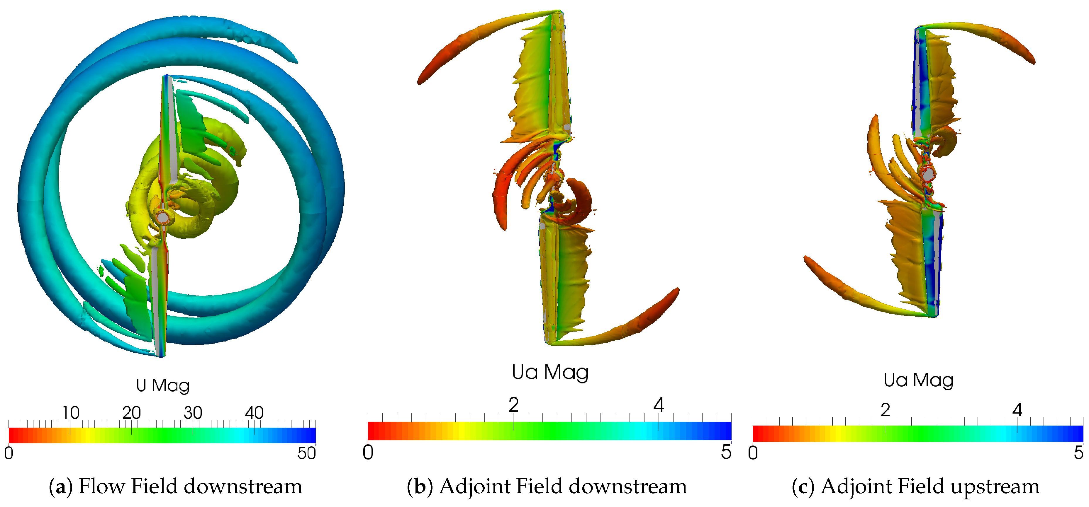
In order to show the flow around the blades in its rotational component, the Q-criterion in terms of the vorticity was used in Figure 4.
The shown flow structures then are colored by the magnitude of the flow velocity and the adjoint velocity, respectively. The computations were performed for both the flow and adjoint velocity. As the adjoint field moves upstream, both views of the rotor are shown for the adjoint field. One view is in the downstream direction, according to the view for the flow field and one is in the upstream direction according to the propagation of the adjoint field. In Figure 4a, the tip and root vortex of the rotor can be seen, as well as low velocities close to the stagnation point and increasing velocities towards the tip of the blade. The tip and root vortex impair the flow field convergence at the root and tip area of the blade, respectively. The computed flow variables are less stable and reach inferior convergence in stationary simulations due to the instationary flow phenomena. As the gradients are evaluated along the movable part of the blade, which are according to Table 1 starting at 2 m spanwise and reach up to m of the span, the influence of the vortices is supposed to be small for the gradient computation. In Figure 4b, it can be seen that similar vortex structures are built for the adjoint field, whereas they are moving upstream and rotating in the other direction compared to the flow field. Figure 4c shows the adjoint field looking at the suction side of the rotor. The large adjoint velocities at the suction side can be seen. In addition, the influence of the tip and root vortex, leading to a reduced adjoint velocity at the tip and root of the blade, respectively, is evident. Large and small adjoint velocities transfer to large and small gradients, respectively. Thus, large adjoint velocities indicate areas of the shape, where changes of the geometry are the most immediate. Overall, the implemented MRF approach for the adjoint field works in a stable manner and allows the computation of adjoint approach based gradients for rotating geometries, and the implemented version shows results expected from theory.
4.2. Convergence Behavior of the Optimizations
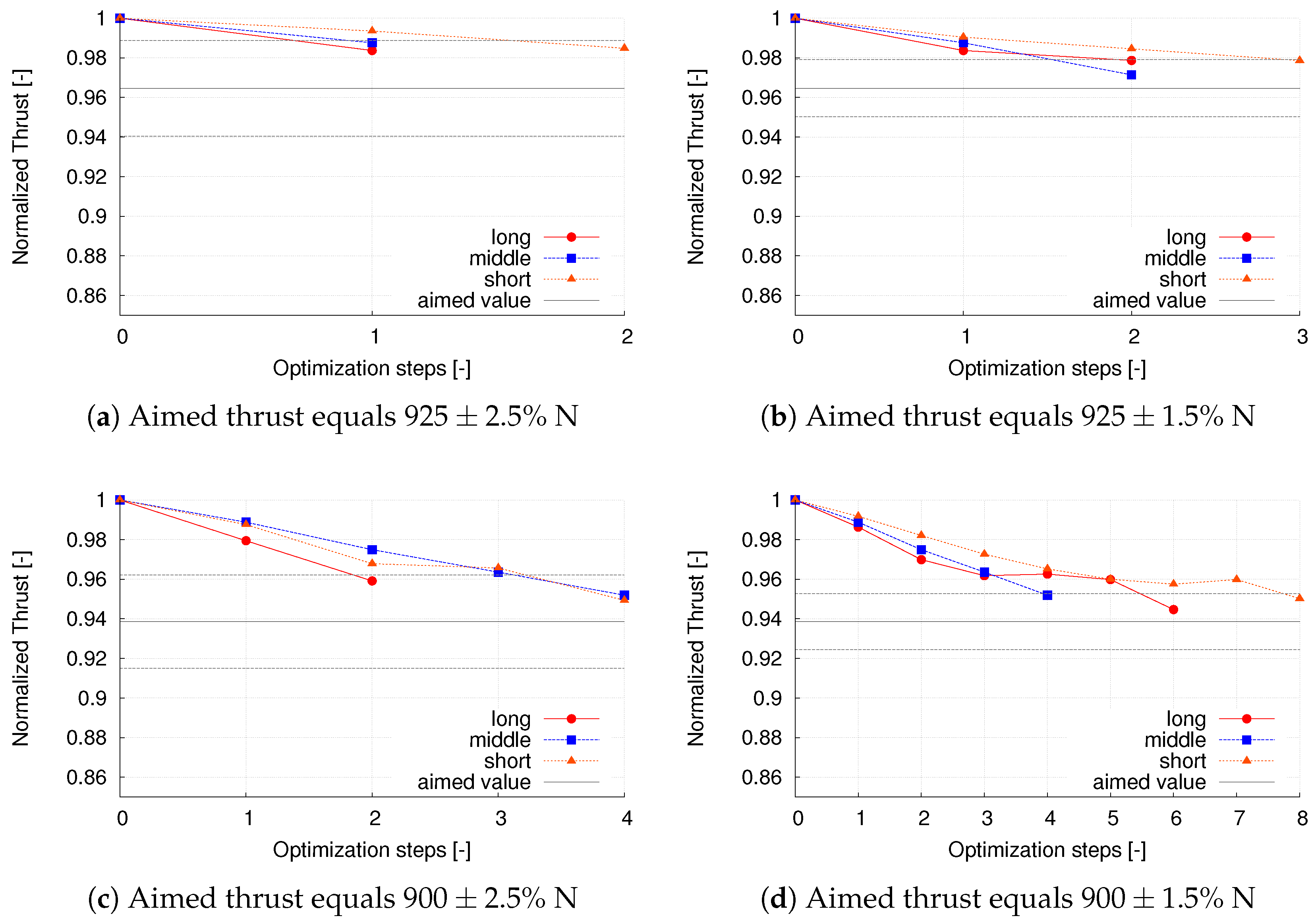
In this work, different types of convergence are used. Numerical convergence of the computed fields is investigated as well as convergence of the optimization tool. Convergence criteria for the flow field are mentioned in Section 3. The latter is defined depending on the ratio between current cost function value and aimed cost function value. The convergence behavior of the various optimizations for different aimed values and varying lengths of the twistable part of the blade is compared in Figure 5a–d.
For all plots, the linear lines between the points are added to ease the following of the trend, whereas only the dots represent computed values of the actual geometries of the blade during the optimization. The thrust is normalized by the initial value of N to ensure comparability of the different aimed values and convergence ranges. The aimed values equal 925 N for the upper plots (a) and (b) and 900 N for the lower plots (c) and (d). The left plots are for the wider allowed range of around the aimed value, whereas the right plots are for a range of around the aimed value.
All optimizations, besides the short and long blade parts for an aimed value of N, show a similar behavior. With each optimization step, the thrust is reduced until the upper limit of the allowed aim range is met. The two named exceptions show a zig-zagging behavior close to the bound, which is a known problem of steepest descent.
Comparing all optimizations, it can be seen that more optimization steps are needed when the aim is further away from the initial value and when the bounds are closer. Furthermore, longer movable blade parts lead to faster convergence, except for the case shown in Figure 5d. In this case, the middle length converges faster than the long length case. It was expected that longer blade parts lead to faster convergence of the optimization as larger parts of the blade are moved relatively to the inflow angle, which then has larger influence on the forces, respectively. For the case shown in Figure 5d, the sensitivity of the optimization process with respect to the user’s input, like initial step-size and pre-convergence of the flow and adjoint field, was found to be the largest. This explains the outlier of the long radial section compared to .
It has to be remembered that each optimization step represents a larger amount of CFD iterations, which are necessary to compute reliable gradients via the adjoint approach. For a convergence after four optimization steps, e.g., shown for the short and middle length in Figure 5c and the given pre-convergence iterations and iterations between two optimization steps specified in Section 3, this sums up to 54,500 CFD iterations per optimization. Roughly 35,000 of these iterations include solving two fields. These numbers are still very convincing for gradient based optimization based on CFD.
When the optimizations for these cases were conducted, a dependence of the convergence, appearance of zig-zagging and initial step-size were observed. As mentioned in Section 2.2, the projected gradients are normalized by the current maximal value. These normalized gradients are then multiplied by the step size, such that the maximal gradient leads to a movement according this step size and the further design points move less. Once converged, optimizations could be sped up by changing the step-size. This is shown in Figure 6 for the long blade part when the aimed thrust equals N.
The two step sizes (red) and (blue) are compared. The larger step size leads to a faster decrease of the thrust within the first steps, but then zig-zagging happens for 14 optimization steps before convergence is reached. The case with the lower step size shows zig-zagging for two steps, before convergence is reached.
This underlines one major drawback of the continuous adjoint approach, also reported in other publications [26,27]. The user input, e.g., initial step size and set-up of the underlying flow simulation, is highly important for these optimizations, whereas other methods are more robust. Still, the shown amount of needed CFD iterations also underlines the advantage of this approach, which is its independence from the amount of design parameters. This still holds for the large Reynolds numbers and rotating geometry investigated in this work.
4.3. Additional Twist Computed by the Optimization
The final additional twist of the blade for the various optimization cases is shown in Figure 7a–c. The dots represent the moving element nodes where the gradients of each element are projected on (see Figure 1). The lines represent the smoothed movement between the nodes, as the geometry movement is also smoothed by the optimization tool. This plotted twist is then added to the initial twist of the according blade. The shown twist are the final ones, summed up over all optimization steps.
All twist values increase from the first element node towards a maximal value close to a spanwise position of 4 m. Afterwards, the additional twist decreases and even reaches negative values for the last element. The positive values in this set-up lead to a reduced angle of attack.
In general, those plots all show two trends: the shorter the movable section, the larger the additional twist. Furthermore, the more restrictive the aimed value, the more deformation is necessary to reach this value. This verifies the developed tool for optimizing rotating rotor blades.
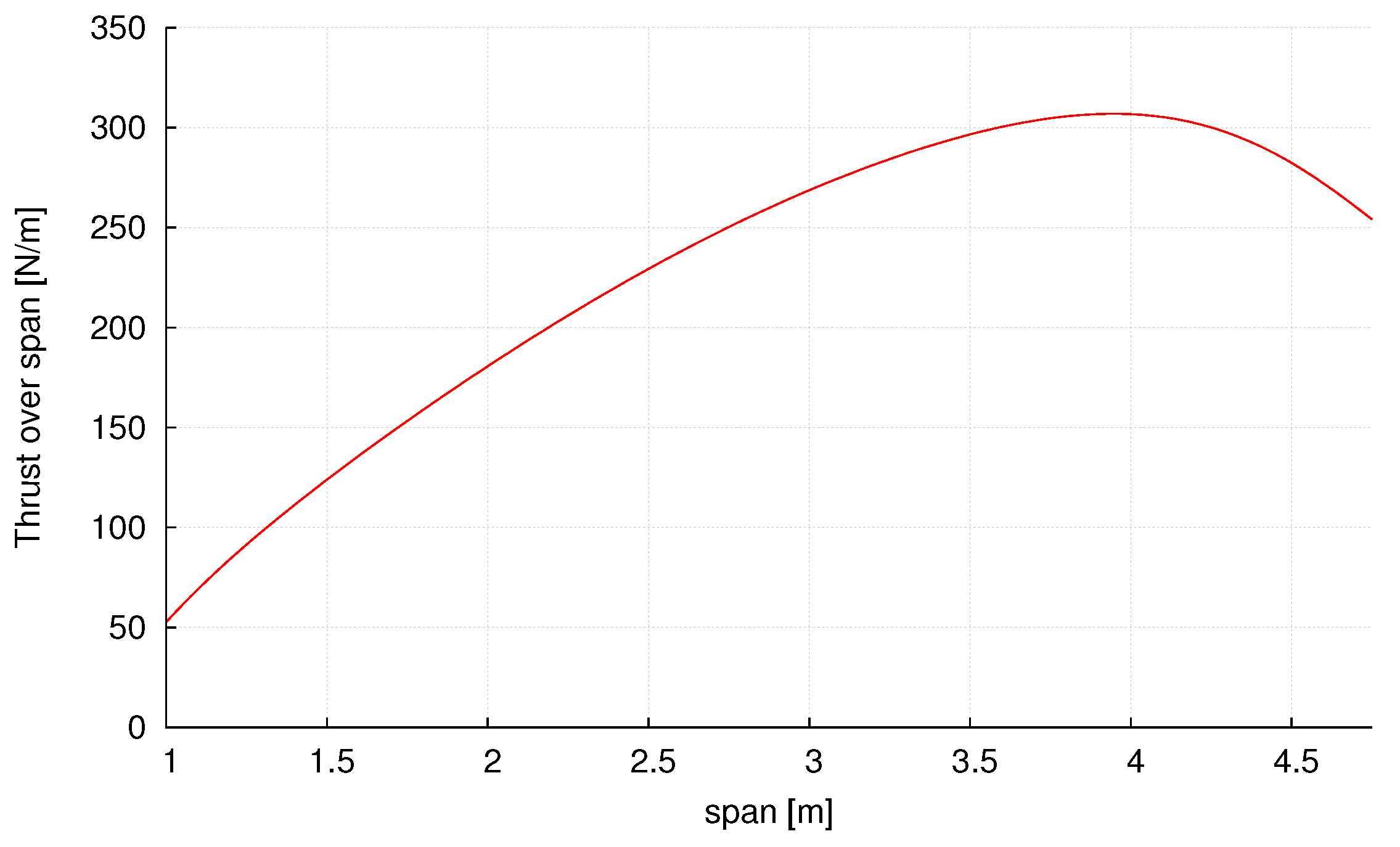
To investigate this behavior further, the spanwise production of thrust of the initial NREL Phase VI blade is plotted in Figure 8.
It can be seen that the thrust production increases in the spanwise direction until a peak at a radial position of m. Afterwards, the production of thrust decreases. Thus, the gradients follow the trend of production of thrust in size and direction, leading to a larger deformation around m and decreased deformation towards the tip.
Larger movements in the outer blade part, which are aerodynamically more efficient, also have a larger impact on the thrust. This is apparently also represented by the gradients leading to a larger deformation in the outer regions. Close to the tip of the blade, the vortices seem to destabilize the adjoint field and thus also the accuracy of the computed gradients. This is also underlined by the larger negative twist values, which where not expected beforehand, of the short deformable blade part in comparison to the two longer ones. The deformable blade part ends at m, whereas the other two deformable blade parts and end at m. Thus, the influence from the tip vortex seems to be stronger for , which reaches m further towards the tip.
The conducted optimizations are chosen to test the developed optimization tool. It is therefore important to reduce the occurring effects as far as possible and avoid converse effects that could arise when using cost functions based on various force components and constraints. For future applications of the developed tool, it is a challenge to extend this method to more important design constraints and more elaborate definitions of the cost function.
5. Conclusions
An optimization tool for rotating wind energy rotor blades at realistic Reynolds numbers was developed and implemented based on the adjoint approach in OpenFOAM. In this work, it was tested for the NREL Phase VI blade. The rotation is represented using the MRF method, both for the flow and adjoint field. A projection for gradients to nodes similar to beam nodes in FSI tools was developed and implemented. This optimization tool is very flexible with respect to the cost function and other optimization settings, using the same dictionary-based input as OpenFOAM.
In this work, the cost function is a least square of the thrust and various aimed values and allowed ranges for the cost function were defined. The different test cases were used to test the stability and convergence behavior of the developed optimization tool. Defining a rather easy cost function allows for interpreting the optimization results based on rotor blade theory.
The 12 test cases all converged within a reasonable amount of CFD iterations. It was found that pre-convergence of both the flow and adjoint field is absolutely necessary in order to achieve usable gradient information. Still, a large influence of the chosen step size for the evaluation of the gradients was observed. This effect got more evident with aimed values further away from the initial value and tighter ranges around this aimed value. An initial study for a range of step sizes, which leads to good convergence behavior, might help to avoid zig-zagging. In the future, gradients can be used in more efficient optimization algorithms like SQP or Quasi-Newton. These algorithms also avoid zig-zagging that can appear when purely following the gradient direction. In addition, known implementations of these algorithms already have an automatized adjustment of the step sizes in run time.
In addition, an adjoint turbulence model is a promising approach to increase the quality of the gradients in future work and thereby the optimization convergence and stability. Using this tool for a blade of a turbine that is not stall regulated could perform better with respect to convergence of the flow and adjoint field.
The applicability of the developed tool, even for a challenging test case based on a rotating, stall regulated turbine at high Reynolds numbers, was shown in this work. When the suggested improvements of the gradient estimation are applied, the optimization tool is expected to perform in a more stable manner. This will allow the usage within the design process—for example, using more elaborate cost functions and being under consideration of constraints.
Author Contributions
Conceptualization, L.V.; Methodology, L.V. and B.S.; Software, L.V.; Writing—Original Draft Preparation, L.V.; Writing—Review and Editing, J.P.; Supervision, J.P.; Project Administration, B.S.
Funding
This research received no external funding.
Acknowledgments
For the simulations, we use the high performance computing cluster Eddy of the University of Oldenburg [28].
Conflicts of Interest
The authors declare no conflict of interest.
References
- Gasch, R.; Twele, J. Wind Power Plants, 2nd ed.; Springer: Berlin/Heidelberg, Germany, 2012; ISBN 3-642-22938-1. [Google Scholar]
- Mücke, T.; Kleinhans, D.; Peinke, J. Atmospheric turbulence and its influence on the alternating loads on wind turbines. Wind Energy 2011, 14, 301–316. [Google Scholar] [CrossRef]
- Kumar, Y.; Ringenberg, J.; Depuru, S.; Devabhaktuni, V.K.; Lee, J.W.; Nikolaidis, E.; Andersen, B.; Afjeh, A. Wind energy: Trends and enabling technologies. Renew. Sustain. Energy Rev. 2016, 53, 209–224. [Google Scholar] [CrossRef]
- Fedorov, V.; Berggreen, C. Bend-twist coupling potential of wind turbine blades. J. Phys. Conf. Ser. 2014, 524, 012035. [Google Scholar] [CrossRef] [Green Version]
- Berry, D.T.A. Design of 9-Meter Carbon-Fiberglass Prototype Blades: CX-100 and TX-100; Sandia National Laboratories: Livermor, CA, USA, 2007.
- Ashwill, T. Passive Load Control for Large Wind Turbines. In Proceedings of the 51st AIAA/ASME/ASCE/ AHS/ASC Structures, Structural Dynamics, and Materials Conference, Orlando, FL, USA, 12–15 April 2010. [Google Scholar]
- Soto, O.; Löhner, R. On the computation of flow sensitivities from boundary integrals. In Proceedings of the 42nd AIAA Aerospace Sciences Meeting and Exhibit, Reno, NV, USA, 5–8 January 2004. [Google Scholar]
- Othmer, C.; de Villiers, E.; Weller, H. Implementation of a continuous adjoint for topology optimization of ducted flows. In Proceedings of the 18th AIAA Computational Fluid Dynamics Conference, Miami, FL, USA, 25–28 June 2007. [Google Scholar]
- Othmer, C. Adjoint methods for car aerodynamics. J. Math. Ind. 2014, 4, 6. [Google Scholar] [CrossRef]
- Soto, O.; Löhner, R.; Yang, C. A stabilized pseudo-shell approach for surface parametrization in CFD design problems. Commun. Numer. Methods Eng. 2002, 18, 251–258. [Google Scholar] [CrossRef]
- Anderson, W.; Venkatakrishnan, V. Aerodynamic design optimization on unstructured grids with a continuous adjoint formulation. In Proceedings of the 35th Aerospace Sciences Meeting and Exhibit, Reno, NV, USA, 6–9 January 1997. [Google Scholar]
- Grasso, F. Usage of Numerical Optimization in Wind Turbine Airfoil Design. J. Aircr. 2011, 48, 248–255. [Google Scholar] [CrossRef]
- Liu, Y.; Yoshida, S. An extension of the Generalized Actuator Disc Theory for aerodynamic analysis of the diffuser-augmented wind turbines. Energy 2015, 93, 1852–1859. [Google Scholar] [CrossRef]
- Jamieson, P. Generalized Limits for Energy Extraction in a Linear Constant Velocity Flow Field. Wind Energy 2008, 11, 445–457. [Google Scholar] [CrossRef]
- Schramm, M.; Stoevesandt, B.; Peinke, J. Lift Optimization of Airfoils using the Adjoint Approach. In Proceedings of the EWEA 2015, Europe’s Premier Wind Energy Event, Paris, France, 17–20 November 2015. [Google Scholar]
- Schramm, M.; Stoevesandt, B.; Peinke, J. Simulation and Optimization of an Airfoil with Leading Edge Slat. J. Phys. Conf. Ser. 2016, 753. [Google Scholar] [CrossRef]
- Vorspel, L.; Schramm, M.; Stoevesandt, B.; Brunold, L.; Bünner, M. A benchmark study on the efficiency of unconstrained optimization algorithms in 2D-aerodynamic shape design. Cogent Eng. 2017, 4. [Google Scholar] [CrossRef]
- Othmer, C. A continuous adjoint formulation for the computation of topological and surface sensitivities of ducted flows. Int. J. Numer. Methods Fluids 2008, 58, 861–877. [Google Scholar] [CrossRef]
- Ferziger, J.; Peric, M. Computational Methods for Fluid Dynamics; Springer: Berlin/Heidelberg, Germany, 2001. [Google Scholar]
- Papadimitriou, D.; Giannakoglou, K. A continuous adjoint method with objective function derivatives based on boundary integrals, for inviscid and viscous flows. Comput. Fluids 2007, 36, 325–341. [Google Scholar] [CrossRef]
- Dose, B.; Rahimi, H.; Herráez, I.; Stoevesandt, B.; Peinke, J. Fluid-structure coupled computations of the NREL 5MW wind turbine blade during standstill. J. Phys. Conf. Ser. 2016, 753, 022034. [Google Scholar] [CrossRef] [Green Version]
- Nocedal, J.; Wright, S. Numerical Optimization; Springer: Berlin/Heidelberg, Germany, 2006. [Google Scholar]
- Hand, M.M.; Simms, D.; Fingersh, L.; Jager, D.; Cotrell, J.; Schreck, S.; Larwood, S. Unsteady Aerodynamics Experiment Phase VI: Wind Tunnel Test Configurations and Available Data Campaigns; National Renewable Energy Laboratory: Golden, CO, USA, 2001. [Google Scholar]
- Tangler, J.L.; Somers, D.M. NREL Airfoil Families for HAWTs; Citeseer: Pennsylvania, PA, USA, 1995. [Google Scholar]
- Rahimi, H.; Daniele, E.; Stoevesandt, B.; Peinke, J. Development and application of a grid generation tool for aerodynamic simulations of wind turbines. Wind Eng. 2016, 40, 148–172. [Google Scholar] [CrossRef]
- Giles, M.B.; Duta, M.C.; Müller, J.D.; Pierce, N.A. Algorithm Developments for Discrete Adjoint Methods. AIAA J. 2003, 41, 198–205. [Google Scholar] [CrossRef] [Green Version]
- Müller, J.D.; Cusdin, P. On the performance of discrete adjoint CFD codes using automatic differentiation. Int. J. Numer. Methods Fluids 2005, 47, 939–945. [Google Scholar] [CrossRef]
- HPC Cluster EDDY of the University of Oldenburg. Available online: https://www.uni-oldenburg.de/en/school5/sc/high-perfomance-computing/hpc-facilities/eddy/ (accessed on 9 July 2018).
Figure 1.
Principle of gradient projection for a wind turbine rotor blade.

Figure 2.
Numerical grid. The flow is coming from the left in (a). In (b), the o-type mesh around a cut through the blade is shown.
Figure 2.
Numerical grid. The flow is coming from the left in (a). In (b), the o-type mesh around a cut through the blade is shown.

Figure 3.
Magnitude (Mag) of the velocity U and adjoint velocity around the blade at a cut at 3 m of the span.
Figure 3.
Magnitude (Mag) of the velocity U and adjoint velocity around the blade at a cut at 3 m of the span.
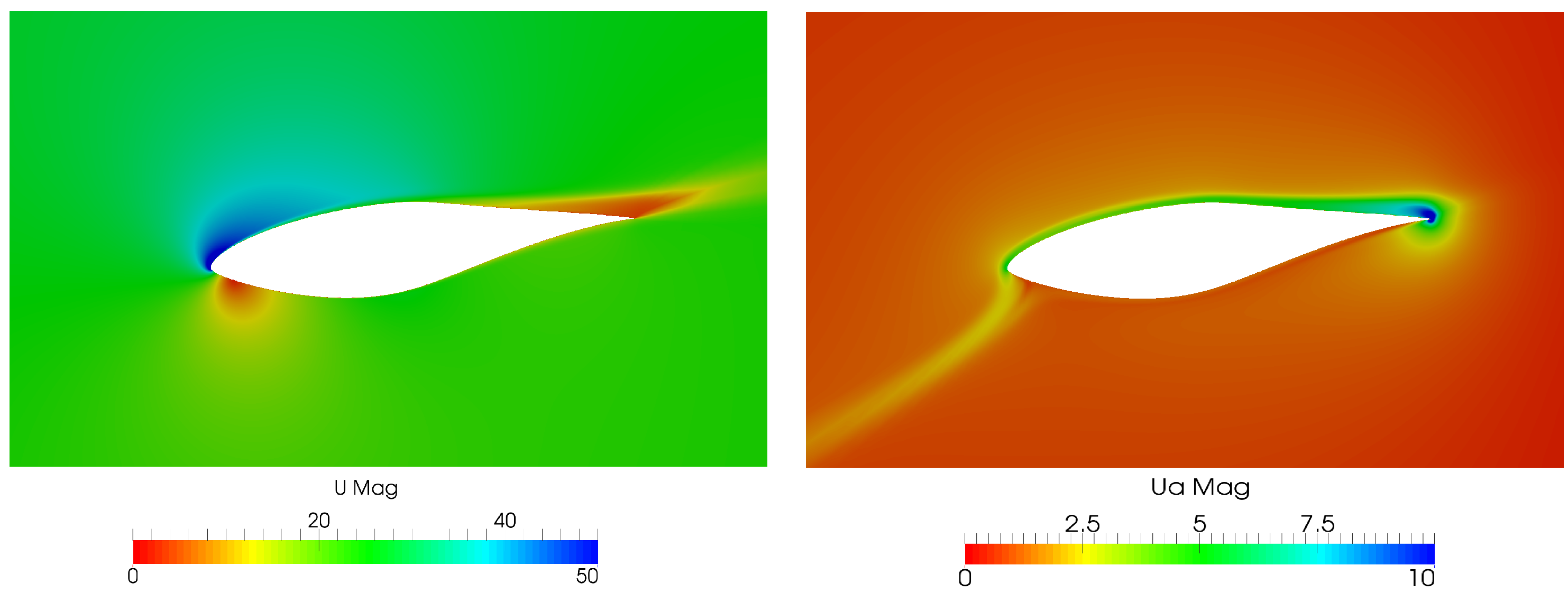
Figure 4.
Field visualisation based on the Q-criterion in terms of vorticity. The full rotor for the flow field in (a) and for the adjoint field in (b,c) is shown. For good comparability, the adjoint field is shown in (b) in the same direction, as the flow field, i.e., downstream. As it moves upstream, it is secondly shown in the direction of the propagation of the adjoint field in (c).

Figure 5.
Development of the normalised thrust force over the optimization steps for design parameters within varying parts of the blade. Long: 2 m–4.5 m radial position, middle: 3 m–4.5 m radial position and short: 3.75 m–4.75 m radial position. The aimed values and the limits of the allowed range are shown with black and grey lines, respectively.

Figure 6.
Development of the normalised thrust force over the optimization steps for the long blade part. The aimed force is N and the initial step sizes are (red dots, StSz1) and (blue squares, StSz2).
Figure 6.
Development of the normalised thrust force over the optimization steps for the long blade part. The aimed force is N and the initial step sizes are (red dots, StSz1) and (blue squares, StSz2).
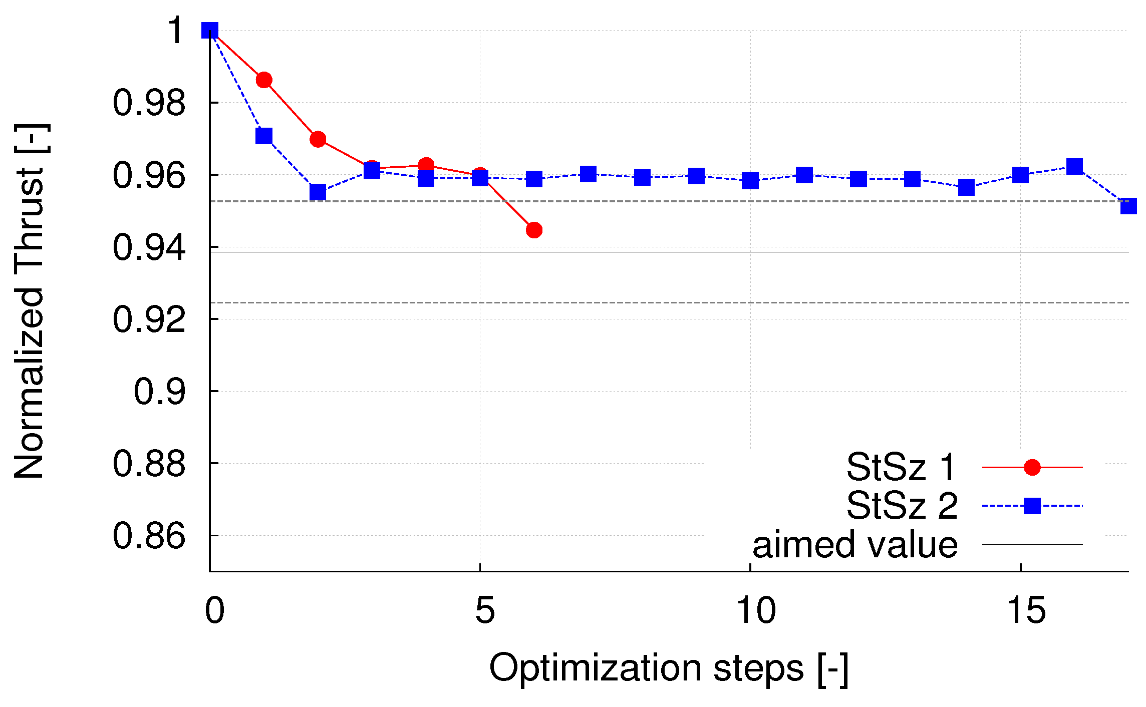
Figure 7.
Development of the normalized thrust force over the optimization steps for design parameters within varying deformable parts of the blade. Long: = 2 m–4.5 m radial position, middle: = 3 m–4.5 m radial position and short: = 3.75 m–4.75 m radial position.
Figure 7.
Development of the normalized thrust force over the optimization steps for design parameters within varying deformable parts of the blade. Long: = 2 m–4.5 m radial position, middle: = 3 m–4.5 m radial position and short: = 3.75 m–4.75 m radial position.
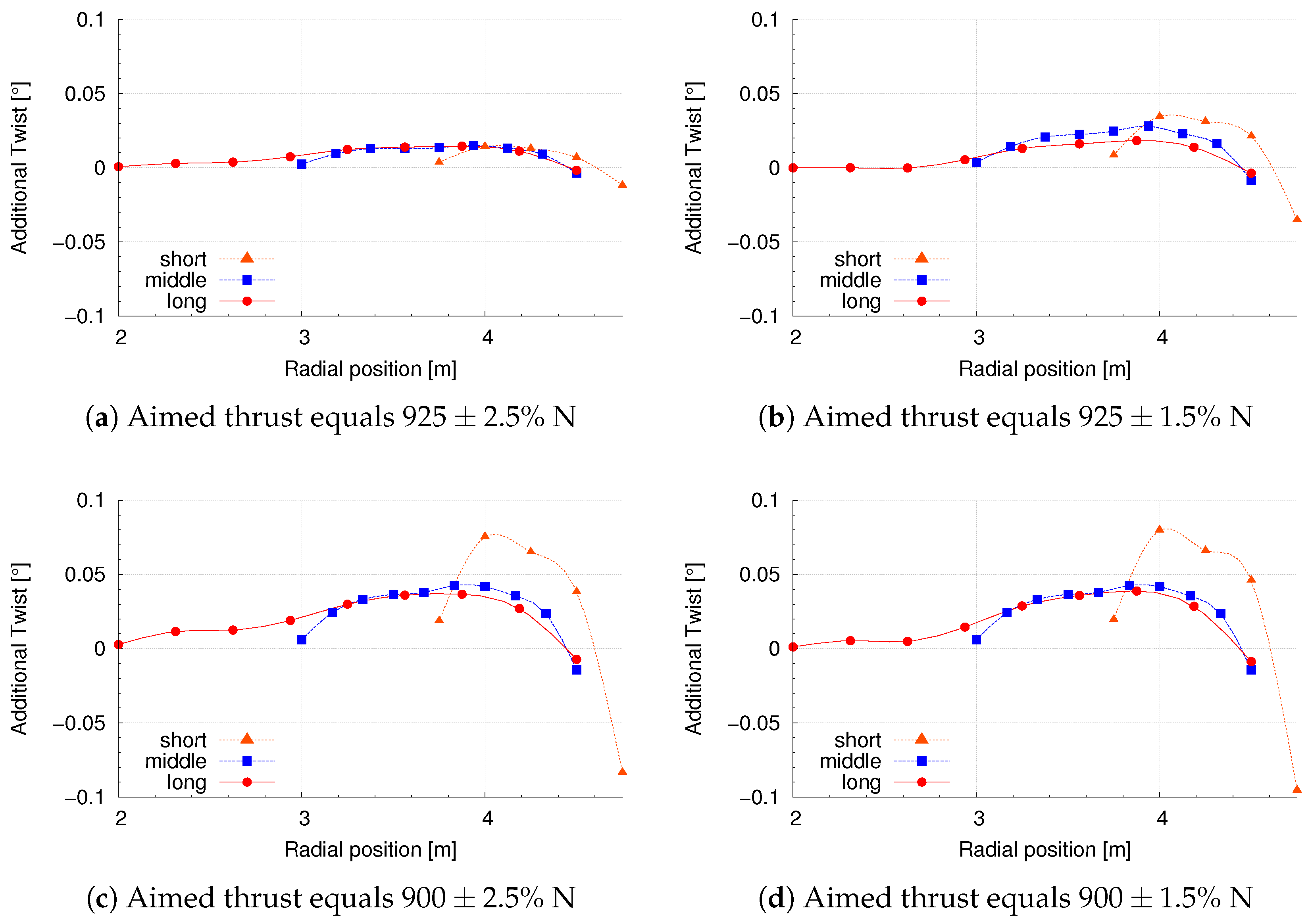
Figure 8.
Spanwise production of thrust of the original NREL Phase VI blade from 1 to m in radial direction.
Figure 8.
Spanwise production of thrust of the original NREL Phase VI blade from 1 to m in radial direction.


Table 1.
Optimization set-ups for different parts of the blade, aimed values and convergence interval around the aimed value.
Table 1.
Optimization set-ups for different parts of the blade, aimed values and convergence interval around the aimed value.
| Case | Convergence Interval | Radial Part r | Blade Part | Length | ||
|---|---|---|---|---|---|---|
| (N) | % | (N) | (m) | % | (m) | |
| 1 | 900 | 1.5 | 886.5–913.5 | 2–4.5 | 50 | 2.5 |
| 2 | 3–4.5 | 30 | 1.5 | |||
| 3 | 3.75–4.75 | 20 | 1 | |||
| 4 | 2.5 | 877.5–922.55 | 2–4.5 | 50 | 2.5 | |
| 5 | 3–4.5 | 30 | 1.5 | |||
| 6 | 3.75–4.75 | 20 | 1 | |||
| 7 | 925 | 1.5 | 911.125–938.875 | 2–4.5 | 50 | 2.5 |
| 8 | 3–4.5 | 30 | 1.5 | |||
| 9 | 3.75–4.75 | 20 | 1 | |||
| 10 | 2.5 | 901.875–948.125 | 2–4.5 | 50 | 2.5 | |
| 11 | 3–4.5 | 30 | 1.5 | |||
| 12 | 3.75–4.75 | 20 | 1 | |||
© 2018 by the authors. Licensee MDPI, Basel, Switzerland. This article is an open access article distributed under the terms and conditions of the Creative Commons Attribution (CC BY) license (http://creativecommons.org/licenses/by/4.0/).
Share and Cite
MDPI and ACS Style
Vorspel, L.; Stoevesandt, B.; Peinke, J. Optimize Rotating Wind Energy Rotor Blades Using the Adjoint Approach. Appl. Sci. 2018, 8, 1112. https://doi.org/10.3390/app8071112
AMA Style
Vorspel L, Stoevesandt B, Peinke J. Optimize Rotating Wind Energy Rotor Blades Using the Adjoint Approach. Applied Sciences. 2018; 8(7):1112. https://doi.org/10.3390/app8071112
Chicago/Turabian StyleVorspel, Lena, Bernhard Stoevesandt, and Joachim Peinke. 2018. "Optimize Rotating Wind Energy Rotor Blades Using the Adjoint Approach" Applied Sciences 8, no. 7: 1112. https://doi.org/10.3390/app8071112
Note that from the first issue of 2016, this journal uses article numbers instead of page numbers. See further details here.