The Simulation of an Automotive Air Spring Suspension Using a Pseudo-Dynamic Procedure


1
Centre for Mechanical Technology and Automation, Department of Mechanical Engineering, University of Aveiro, 3810-193 Aveiro, Portugal
2
Aveiro Research Centre of Risks and Sustainability in Construction, University of Aveiro, 3810-193 Aveiro, Portugal
*
Author to whom correspondence should be addressed.
Appl. Sci. 2018, 8(7), 1049; https://doi.org/10.3390/app8071049
Submission received: 25 April 2018
/
Revised: 6 June 2018
/
Accepted: 15 June 2018
/
Published: 27 June 2018
(This article belongs to the Special Issue Soft Computing Techniques in Structural Engineering and Materials)
Abstract
:This paper describes a numerical solution to characterize the deformation of a bellows-type air spring for automotive suspensions. In a first step, the shell structure is modeled as a practically inextensible membrane that has virtually no bending stiffness; the structure has only a pneumatic-elastic deformation due to the compressibility of the pressurized air. In a second step, a finite element modeling of the device using a commercial code is carried out in order to validate the first model. Complementing this work, an experimental procedure based on a pseudo-dynamic technique was implemented to simulate the behavior of the pneumatic suspension bellows subjected to dynamic loads. The method consists of a combined numeric/experimental procedure simulating a suddenly applied load.
1. Introduction
The historical development of vehicle suspensions equipped with pneumatic spring elements has a remarkable temporal extension. A considerable number of projects or devices have appeared due to inventors who have expected to contribute to the smoother running of vehicles for a long time, either for road or railway applications. In this work, a brief review of the technical history of the theme is based principally on the published technical literature.
Actual communications about the design and testing of pneumatic suspensions tend to be currently presented in a resume format, which is normally aimed at advertising by manufacturers and designers, who want to signify their engineering progress. On one hand, this option possibly has restrictions for research diffusion strategies. On the other hand, data about fatigue analyses is also available in specific technical journals by manufacturers, who have spent some time testing their automotive transportation products under real long-term road driving conditions. Such studies are more focused on meeting the confidence of vehicle drivers and experts on vehicle maintenance, rather than the diffusion of detailed research in specific scientific and technical publications.
It seems that the earliest known report about the project of a pneumatic suspension is that of Humphreys [1], who required patent No. 673682 for the proposal of a suspension design combining front and rear arched leaf springs with a pair of long cylinders filled with compressed air and connected to the arch leaf springs in a serial arrangement, as depicted in Figure 1. The technical description of the system is practically restricted to the basic concept and operating principles, with no calculation or formula for the spring stiffness and stroke. Another early historical development of this suspension concept that is much more recent than that of Humphreys [1] was published by Sainsbury [2]; this one had some technical detail, describing the essential air circuit architecture, components, and quantitative settings of a pneumatic suspension for production. By 1950 onwards, air suspensions experienced a large development as many transportation companies decided to implement those suspension systems in their vehicles, which resulted in quiet and smooth running.
The actual performance of automotive bellows suspension has reached an important technologic standard through the implementation of pressure/stability control electronic hardware in railway coaches, as reported by Quaglia and Sorli [3].
Normally, the structural analysis and dynamic testing of bellows air springs are not presented with detail due to manufacturers’ strategic restriction of technologic knowledge dissemination; alternatively, university institutions working in automotive engineering share valuable contributions. Examples can be assigned to Löcken and Welsch [4] (from Helmut Schmidt University, DE), who studied the dynamics of bellows air suspensions accounting for the coupled effect of air heating and spring stiffness increase by the coupled effect; the natural frequencies and damping methods were also studied. The shape of the elastic element considered by Löcken and Welsch [4] was not a toroidal shell like the one analyzed in the present work. Such a shape conditioned the spring geometry by the mutual surface contact of the elastomeric membrane and the internal rigid core, giving rise to the non-linear kinematics contact model in the numerical modeling.
Among the finite element models of deformable shells conducted so far, it is worth mentioning the one presented by Yilong Zhang et al. [5], who modeled suspension bellows as toroidal shells with a coupling of the prescribed deformation and the internal pressure, having used ANSYS® for the purpose. The objective was to obtain the natural frequencies of a suspension for several internal pressures, verify the non-linear behavior, and implement linearization methods to solve the problem of the evaluation of natural frequencies.
Air spring suspensions are mounted in a large number of railway or roadway vehicles and have been a technical success, given their reliable, functional, and robust design. Urban vehicles equipped with pneumatic suspensions can travel with a constant vehicle-to-ground level independent of the payload; moreover, in urban buses, it is possible to tilt the vehicle slightly about the main axis to make the passengers’ entrance or exit easier; finally, a quite smooth running can be taken with this engineering solution with the availability of the spring stiffness selection control according to the road condition and the driver’s preferences. Figure 1 sketches an example of an actual engineering solution for® air spring suspension.
A most common engineering design for composite structure bellows air springs (steel braid and synthetic rubber polymer matrix) is depicted in Figure 2.
This spring consists of two or more toroidal-shaped shells enclosing pressurized gas (normally air). The static pressure determines the mechanical characteristic equivalent to a spring with a pre-set load prior to the deformation from externally applied compression forces. The air spring has a non-constant spring rate, a parameter that also depends on the deformation velocity as analyzed ahead. The development of these accessories is mainly a result of numerical and experimental research with models reproducing the on-road behavior of air springs when mounted in the vehicle suspension as accurately as possible. It is expected that such research is mainly presented by the manufacturers of pneumatic components for road and railway transportation.
The present work focuses on a suspension system (as exemplified in Figure 1) that allows a dynamic analysis in a real-time process using a test rig with dynamic actuators. Alternatively, a pseudo-dynamic method can be implemented, as described in the next section of this work.
2. The Air Spring Stiffness
2.1. The Displacement Field of the Toroidal Shell
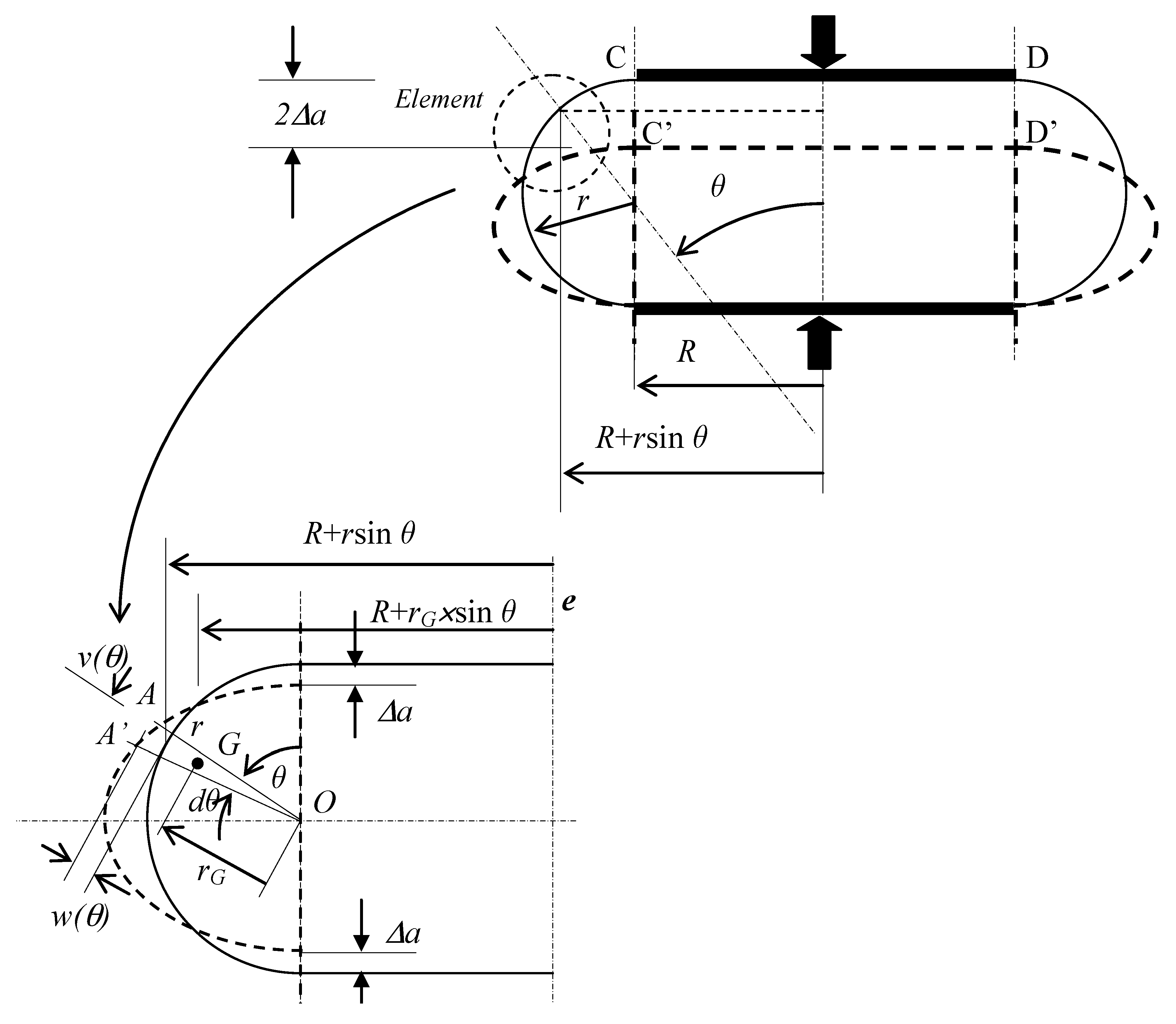
Pneumatic springs for automotive applications work mainly under compression forces. Conventionally, such forces and the respective axial displacements are considered positive. The pneumatic stiffness relates the spring response to the prescribed displacements along the axis. A numerical solution is developed to define the constitutive relation of the shell deformation versus the axially applied load. As the elastic element is compressed air, the pneumatic stiffness will depend mainly on thermodynamic factors, e.g., the deformation rate, given the quasi-adiabatic transformations expected. The deformed shape of the shell is obtained upon assuming membrane inextensibility along the shell principal curvature directions. Figure 3 sketches how the toroidal bellows behaves under the external load. Two modules of area are affected by the internal pressure in the spring deformation work: the toroidal bellows surface and the flat circular piston (marked as CD in Figure 3), which is eventually bolted to the vehicle suspension arms or frame body.
The following parameters characterize the shell geometry:
- r is the meridian radius
- θ is the meridian angle
- R is the longitudinal (or circumferential) radius
- w is the transverse (or normal) displacement
- v is the meridian (membrane) displacement. This displacement does not participate in the simplified model to calculate the work done by the internal pressure in the shell deformation.
Considering w(θ) as the relevant displacement to characterize the shell distortion, the incremental work ΔU performed by the internal pressure against a prescribed displacement Δa at both flanged ends is evaluated by the variation of the shell volume. For this, the static moment of an elementary triangle defined by points {A A’ O} with reference to the axis of revolution e must be calculated. Then, the volume of the shell is obtained with the theorem of Pappus–Guldin (in the book of Tom M. Apostol [6]) and integrating the following function for the meridian angular variable θ in interval [0, π]:
The static moment of the elementary triangle {A A’ O} in Figure 3 is obtained from the product of its area by the distance of the mass centre (located at 2/3 of the triangle height) to the axis of revolution e. Volume increment is due only to transverse displacement w obtained after subtracting from Equation (1) a similar expression but with w = 0:
Considering that the toroidal membrane shell enclosing the compressed air has a circular meridian line and, after being subjected to external forces, the distorted shape of that meridian is approximately trigonometric, then, a simple approximate solution for the transverse and meridian displacements is as follows:
(Displacement v(θ) in Equation (3) ensures the inextensibility along the meridian arch, but is not used in the formulation of the pneumatic stiffness).
where a is a parameter associated with the amplitude of displacement w to be obtained by techniques of variation calculus. Substituting this expression in Equation (2), a practical formula is obtained:
2.2. The Pneumatic Stiffness
In this step, two models are used to approach the mechanical/pneumatic behavior of the spring:
- (a)
- The first model assumes that only the compressed air participates as an elastic body in the evaluation of the spring stiffness. The shell torus enclosing the air does not contribute to the suspension stiffness;
- (b)
- The second model consists in superimposing the structural stiffness of the shell torus to the one of the air under compression, as two springs working in parallel.
In step (a), the spring stiffness due only to the air under compression results from the concept of differential volume contributing to the internal pressure work. The internal energy stored in a pressurized gas enclosed in a volume Vol is given by the integral expression:
which is calculated over the volume of the container. For a small variation ∂a of parameter a, the internal pressure P practically remains unchanged. For an axial compression of the toroidal bellows, the variation of the internal energy U is, from Equation (4), given by:
By the theorem of virtual work, the force associated with the internal energy rate due to a virtual ∂a is obtained as follows:
(It is noted that there is a pair of symmetrical forces applied to the flanges of the spring; hence, the differentiation in order to the double value ∂(2a) of the amplitude increment).
The calculation of the tangent stiffness associated with the variation of the spring compression force in Equation (7) is also obtained by considering the double variation ∂(2a) of the relative displacement of the flanges:
From the expression in Equation (7), the tangent stiffness of the pneumatic spring is:
where Vol is the current total shell volume as in Equation (1) using the expressions in Equation (3).
The calculation of the variation rate of the current pressure P with the volume Vol due to the displacement a depends on the thermodynamics law of the air; as the spring is generally subjected to high speed volume changes, then it is coherent to assume an adiabatic law for the pressure/volume variation of the air enclosed in the bellows shell:
where γ is the adiabatic exponent, and variables with subscript 0 refer to the initial values of the pressure and the volume; then:
The minus sign in the previous expression is due to the antagonist variations of the pressure and the volume, either in isothermal or adiabatic transformations. Here, an absolute value was assumed for the purpose of obtaining a normalized value for the pneumatic stiffness of the spring exclusively in compression. Generally, γ ranges from 1.2 to 1.4 (perfect gases); in this work, an intermediate value of γ = 1.3 was considered. A complete expression for the pneumatic stiffness can be obtained from the expression:
which depends on a current value of the axial displacement a of the bellows spring. For each displacement increment Δa of the spring, the current force Fa in Equation (7) changes accordingly with a constant value of the stiffness in Equation (12):
Although Ka depends on the air pressure, it is assumed to be constant during the displacement increment referred above. Equation (13) is thus a linearized form to update the structure configuration past an iteration Δa. The next section describes the linearization process of the iterative algorithm to obtain the solution for the structural deformation.
In step (b), the deformation of the torus shell is calculated to be added to the pneumatic stiffness that was previously obtained. This shell is assumed to have very low bending stiffness, while being practically inextensible under membrane forces (as expected with a steel braid-reinforced rubber shell, where only the membrane stiffness is relevant). Figure 3 is used to develop the upcoming calculation. Since the relevant displacements participating in the deformation field of the torus shell were above identified to be w and v, the deformations for the axisymmetric loads are:
The first two terms refer to the linear small displacement deformation models, respectively the longitudinal and the meridian deformations (Ugural [7]), while the third term is the meridian curvature involving a linear term (for small bending displacements) and an additional quadratic term for moderately large bending displacements (Reddy [8]). The non-linearity term only in the curvature expression derives of the low bending stiffness of the shell, allowing expectable large transverse displacements, while other deformation terms are small. The corresponding Hooke’s law for the strain tensor in Equation (14) only involves the longitudinal membrane force and the bending moment as follows:
where [D] is the elasticity matrix containing the Young’s modulus E and the Poisson’s ratio ν of the material, and {ε} is the strain vector. The strain-energy resulting from the axisymmetric loading of the torus is given by:
where θ is the meridian angle and ϕ is the longitudinal angle, which are both parameters in the integration over the shell main curvatures. According with the Castigliano’s theorem, the internal reaction Rshell and associated tangent stiffness KT-shell due to a displacement of magnitude a (the only unknown in Equations (3) and (4)) of the axisymmetric shell are:
This tangent stiffness of the shell deformation is added to the one corresponding to the pneumatic elasticity of the system as obtained above.
2.3. The Equilibrium Equation: The Iterative Newton–Raphson Method
The compression of a pneumatic spring can be numerically evaluated by a non-linear algorithm, where the current stiffness and shell structural configurations are updated at each iteration step. The method can be developed by prescribing the displacement or force increments. The process ends when the final force is obtained inside a tolerance interval of the effective internal reaction force associated with the structure deformation. The pneumatic stiffness is given by Equation (12) for adiabatic (1.4 ≥ γ > 1) or isothermal (γ = 1) transformations. In the calculation of the tangent stiffness Equation (12), r and R are current values that are assumed constant during a deformation iteration of the shell by the axial displacement a. The Newton–Raphson method is used to solve this problem under the following steps:
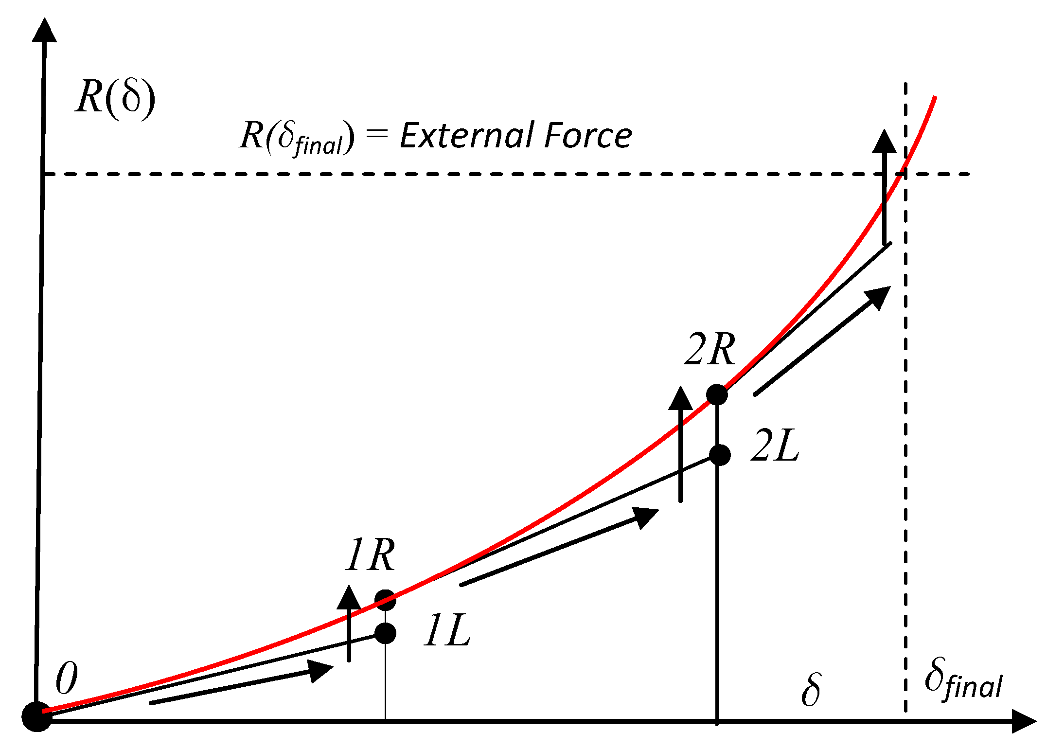
- A continuous function F(a) can be written for an increment of its independent variable a, as F(a + Δa) ≅ F(a)+Δt × F’(a) from the Taylor’s formula up to a first-order expansion. Naming F(a + Δa) = Fn+1 and F(a) = Fn; a + Δa = an+1 and a = an, then, the previous approach is equivalent to: Fn+1 − Fn ≅ (an+1 − an) × F’(a). This formula models a linearized evolution of the structure constitutive relation for displacements inside the interval [a, a + Δa]. Graphically, this equation corresponds to a tangent line at a point of the curve that effectively represents the constitutive behavior of a structure, eventually with elastic, yet also represents the non-linear behavior of the internal reaction force vector from a prescribed displacements vector, as sketched in Figure 4. As point F(a + Δa) here obtained does not correspond to the effective reaction of the structure (this one given by Equation (7)), there is a residual difference to the real value, which is a parameter suitable to control the iteration pitch, as depicted in Figure 4.
- The points labeled with “L” result from the linear approach, while points from initial internal reactions are labeled with “R” (Figure 4). Past the iteration, the linearly obtained next value is compared with the effective one, where the difference of effective and linear points is the residual value for the precision control of the iteration. This process is schematically represented by arrows in Figure 4, and is concluded when the final linear value of the internal reaction vector is close to the real one (the external force) by an error smaller than the prescribed tolerance.
2.4. Example of Loading a Single Cell Bellows of a Pneumatic Suspension
The mechanical behavior of a single-cell toroidal bellows (as in Figure 3) that is subjected to a prescribed displacement along the axis of revolution is numerically modeled. The shell geometry and initial stiffness calibration parameters:
- Radius of the meridian line r = 50 mm
- Radius of the circumference line (passing through the center of the transverse meridian circumference) R = 200 mm
- Initial pressure P = 2 bars (≅0.2 MPa)
The bellows is compressed about the axis of revolution up to a stroke of 50 mm (half its initial height). Increments of 2.5 mm are adopted in the Newton–Raphson iteration algorithm. Figure 5 shows graphically the force versus the prescribed displacement of the air spring with the iterative process described above and depicted in Figure 4.
It is noted that each displacement in the graphics of Figure 5 refers to the shell mid-plane due to the deformation symmetry; then, each stroke is double that of the respective displacement in abscissas’ axis.
On compressing the bellows up to half of the initial volume, by the thermodynamics law of perfect gases, the final pressure should be twice the initial one with an isothermal process, and about 2.5 times that with an adiabatic variation; however, this relation does not apply due to the additional air volume of the torus shell membrane, where its variation is not linearly proportional to the axial displacement, as with the ideal cylinder joining both end flanges of the bellows spring (Figure 2 and Figure 3). Differences are assigned, for example, to the variation of the isothermal compression force from 25 KN to 42.5 KN and in the adiabatic compression reaching 47.5 KN, when the shell is compressed to half of its initial height.
This geometric characteristic shows that the additional semi-torus volume can play a useful role in the suspension design for safety and optimal comfort ride on setting the ideal stiffness of air springs.
3. Pseudo-Dynamic Simulation of the Automotive Suspension
3.1. Applications to the Dynamic Analysis of Automotive Suspensions
Automotive suspensions attenuate the vibration of the vehicle body due to road irregularities on run. The dynamics of conventional automotive suspensions refer to a passive transmission model, where the base (road) prescribes a time-dependent displacement and velocity to the equivalent system. This set, comprising tyre, spring, and damper, is the vehicle wheel suspension model having its displacement velocity and acceleration vectors as kinematic parameters. Figure 6 shows a sketch of a suspension with the spring/damper set, but here, the elastic element is a bellows-type air spring in an equivalent dynamic system as a single degree of freedom (SDOF) model. The damper is a device that restricts the suspension amplitude on run with a force that is velocity dependent, as explained below.
In this simplification, the equivalent mass is a part of the total vehicle mass depending on its distribution by the axles. For each wheel, the dynamic model of the automotive suspension can be represented with good accuracy as a SDOF system, provided that the displacement field can be assigned to a dominant value at a defined point. This is the case of the wheel hub, considering the tire stiffness is much larger than the suspension spring, practically transmitting the entire displacement from the road profile to the wheel hub and to the spring end. As indicated in Figure 6b, the base (road) prescribes a displacement U0(t) to the wheel axle (assuming here that the elasticity of the tire is much larger than the spring one), while the equivalent mass M of the vehicle body is displaced U1(t). The dynamic equilibrium of the spring/mass model of Figure 6b is:
where Fspring and Fdamper are the spring and the damper reaction forces due to the relative displacement and velocity between the road profile and the wheel hub. Supposing that the spring has a linear elastic behavior and the damper reaction force is also linear-dependent on the relative velocity, then Equation (18) can be written as:
in this equation, Kt is the spring stiffness (in N/m), and C is the damping constant (in Ns/m), which is a parameter assigned to viscous-type dampers. Constant C has a stable value when the damper is in good condition and is operated at a stabilized temperature. In the present study, a constant value of C is assumed.
Separating in each hand of Equation (19) the force terms of the displacement and velocity of the base and wheel hub, respectively, the passive transmission SDOF equation of the dynamic system is obtained:
The left-hand side of Equation (20) can be interpreted as an external time-dependent equivalent force Fequiv(t) on assuming a virtual profile for a road where the wheel/suspension set travels at a prescribed horizontal velocity. This equation must be integrated numerically with a time integration algorithm as explained below, but for now, it is important to note that the following term on the right-hand side of Equation (20) corresponds to the spring internal reaction force to a prescribed displacement U1(t) at any instant t:
This internal reaction force Rt can be measured with a load cell inserted between one end of the spring and the ram of the displacement actuator mounted in the test rig. The evaluation of the spring stiffness Kt at each time step t is carried out upon recording the consecutive values of the internal reaction force, respectively, at instants t and +Δt calculating the tangent stiffness Kt+Δt by Equation (22):
This calculation is necessary whenever the spring has not a linear elastic mechanical behavior, as is the case of the pneumatic bellows numerically analyzed above. The damping force cannot be measured by means of a static procedure; instead, the damper contribution participates in the time integration algorithm that is described next.
3.2. The Direct Time Integration Algorithm: The Newark Constant Acceleration Method. Application to Pseudo-Dynamic Methods
In structural dynamics, the behavior of a structure is characterized by the displacement, velocity, and acceleration vectors, respectively , , and , the equilibrium being expressed by the equation written for the time step t + Δt:
where {R} is the structure internal reaction vector, and [C] and [M] are, respectively, the damping (viscous type) and mass matrices, which are assumed constant at time step t and during the time increment Δt, while on the right-hand side, {F(t)} is the external force vector. In linear systems, the internal reaction vector is the result of the matrix and vector product:
In a generalized constitutive behavior system, the evolution of this internal reaction vector is given by:
The structure linear stiffness [K]t (from (11-d)) can be assumed to be constant during a deformation increment associated with the time step Δt, in order to develop Newmark’s [9] method, where the stiffness matrix in Equation (25) corresponds to a tangent stiffness during the time increment Δt.
The pseudo-dynamic procedure refers to a sequential process involving data transmission between a numerical model with Equation (1) and an experimental step. In this last step, the measurement of the internal structure force or structural restoring force vector is carried out. Such measured data corresponds to the effective mechanical behavior of the structure at the level of the selected degrees of freedom.
The pseudo-dynamic techniques operate with an implicit time integration algorithm, as is the case of Newmark’s [9] method. To develop the iterative formulation, the expressions of mean acceleration and velocity are used:
Substituting these expressions into Equation (23), having separated the terms at instants t + Δt of those at t, the standard Newmark’s time integration method is obtained:
This expression gives an updated acceleration vector that can generate new velocity and displacement vectors with Equation (23) by the recursive process in Equation (27), approaching the dynamic behavior of the structure. This algorithm has the remarkable potential of ensuring an unconditional convergence, even with relatively large iteration time steps. This does not mean that the solution obtained is necessarily accurate, as this is achieved if the time step is smaller than a critical value given by the formula:
This value represents the decimal fraction of the natural period of a single degree of freedom vibrating structure, which is the case under analysis; in a multi-degree of freedom, the critical value for the time step involves the smallest natural period of the discretized vibrating structure.
3.3. Description of the Method and Application to the Dynamic Analysis
3.3.1. Operation Principles
The pseudo-dynamic method is a sequentially organized procedure, where in an experimental step, a structure model (or test specimen) is subjected to a set of prescribed displacements with precision actuators at the level of the structure of the degrees of freedom. This imposed distortion generates an internal reaction force vector measured with load cells that is fed into the numerical algorithm of the time integration method. These coupled operations integrate a closed loop where the experimental step communicates data to a computer running the time-integration algorithm program; in turn, the computer drives the set of displacement actuators, continuing the process until a pre-defined number of time steps is concluded.
While the internal reaction force vector can be measured in a static process, the viscous damping forces in the structure cannot, as the viscous type damping is proportional to the velocity. However, an exception is assigned to structural damping, with this energy dissipative mechanism resulting from the internal friction forces of the material in deformation. However, such a model does not apply to the system in examination, with viscous damping being the right vibration dissipation model.
Although proportional to the velocity, viscous damping forces can nevertheless be calculated numerically, provided that the damping constant is known. Moreover, viscous damping can be assumed to remain stable during the vibration cycle. For this purpose, Equations (26) is used and damping forces actually participate in updating the dynamic structure status in Equation (27).
3.3.2. Engineering Design of the Rig and Applications
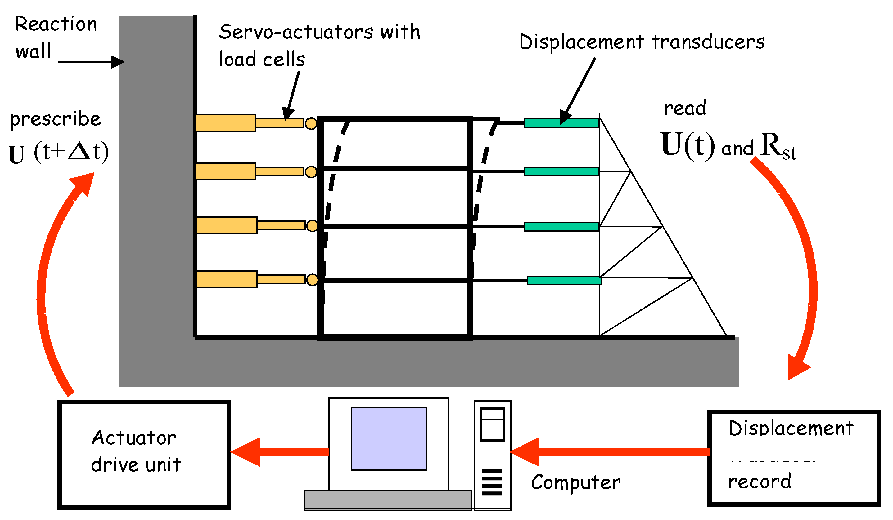
In civil engineering, the assessment of multi-storey structures for seismic safety deals with damage modes occurring mainly by a sway-type mechanism. Such configurations are the result of horizontal displacements associated with the natural vibration modes of the structure. This makes the kinematic principle of pseudo-dynamic methods ideal for the simulation of dynamically stressed structures by seismic disturbances. The design of the test rig, the automation system, and power units make this system a competitive alternative to largely sized seismic tables for real-time dynamic analysis. The primary importance of the engineering field and its applications are evidenced by the research (Pinto et al. [10,11]) performed, for example, in ELSA (European Laboratory for Safety Assessment), a large laboratory facility where real-scale structure models are tested for their seismic safety by pseudo-dynamic analysis.
Figure 7 shows a sketch of a conventional test rig in the simulation seismic loads, where the operating principles of the method are summarized. A rigid reaction wall receives the thrust from the actuators when prescribing a displacement vector to the test specimen. In seismic engineering, it is desirable that full-scale test specimens should be used in dynamic analysis, as reduced scales may not realistically evidence the damage models, given the lesser accuracy in transposing the mechanical properties of the real-size structure material to the one used in reduced-scale test specimens.
While there are recognized advantages of pseudo-dynamic procedures in seismic engineering, in other research areas such as automotive engineering, test rigs do need not to be very large nor afford the high-power capacity as required in seismic analysis; therefore, pseudo-dynamic testing systems are not so competitive as test rigs in real-time dynamic analysis for the following reasons:
- The number of degrees of freedom to obtain accurate results may be predictably high, a less favorable attribute in the design of pseudo-dynamic test rigs;
- The size and engineering complexity of the equipment for pseudo-dynamic testing are not remarkable advantages considering that a real-time dynamic analysis test rig records internal reactions and damping forces. In turn, with pseudo-dynamic methods, viscous damping forces have to be numerically inserted in the time integration algorithm, as referred above.
- The dynamic analysis of some components in the automotive industry cannot be approached only with a set of time-dependent displacements, since the inclusion of nodal rotations in discretized models is necessary. This requirement makes the adequate design of the test rig more expensive, with an additional need of implementing angular transducers, more elaborate test-specimen fixtures, and specific load cells, which is an option that may not guarantee accurate results.
Despite these drawbacks, an apparently favorable feature of the method in the scope of automotive engineering was found by the authors in using a test rig (Figure 8) that was designed for the certification of automobile seats by pseudo-dynamic simulation of the passenger/seat interaction in a crash test analysis (Carneiro et al. [12]). Thanks to the sequenced/incremental process in the test specimen deformation, the progressive collapse of the seat fixing accessories (such as bolts, rivets, and welded joints) could be observed with some detail on setting a pause to the structure deformation and recommencing it when desired. The test rig schematically represented in Figure 8 was a more elaborate version of the one presented by Pinto et al. [12]; however, it was not published, as it was still in development and tests at the date of the present paper’s publication [11].
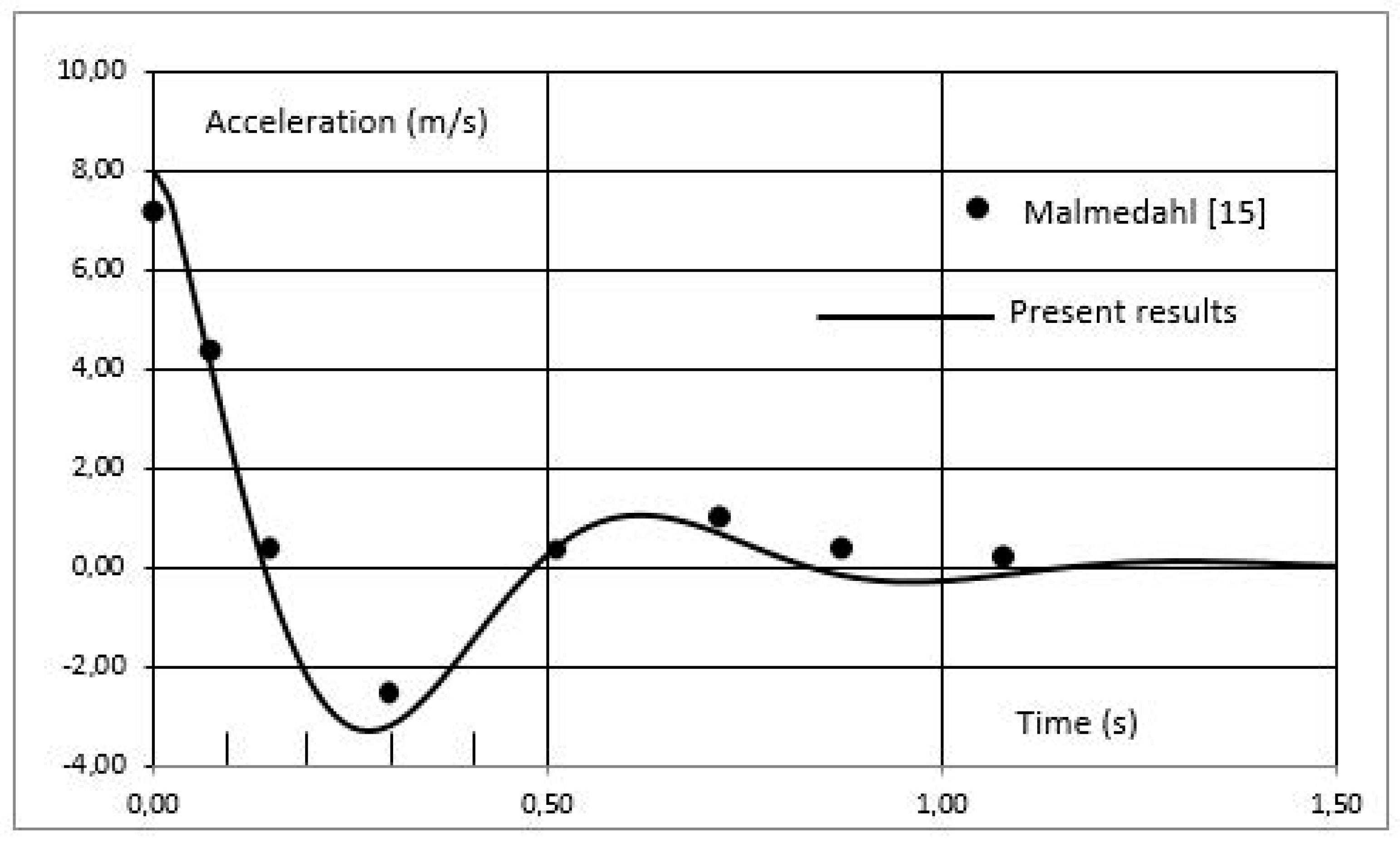
In order to assess the accuracy of Newmark’s method for the time integration algorithm of the pseudo-dynamic analysis, an example related to an automobile suspension test is performed. The example was taken from Malmedahl [13], where the suspension of an off-road vehicle was subjected to the effect of the vehicle dropping from a small height. For that purpose, Malmedahl [13] used a special metallic kink that, once buckled, brought the suspension set to a sudden contact with the ground.
The initial conditions of the problem could not be exactly repeated with the present solution, as the velocity of contact with the soil was not known. To approach the problem with data similar that used by Malmedahl [13], an initial impulsive force was assumed to deform the spring/damper pair, where that force was calculated from the initial acceleration, which was a known parameter. The following data were considered in the problem:
- Sprung mass Ms = 340 kg;
- Damping Constant Cs = 2.25 kNs/m
- Spring Stiffness Ks = 31.2 kN/m.
A step force was applied to the suspension system at instant t = 0; thereafter, the force was steady and stable. The force selected was quantified after setting the initial acceleration a0 = 8 ms−2, at t = 0. Malmedahl [13] probably chose the trigger instant for acceleration time start not necessarily at t = 0, but rather slightly anticipated, as shown in Figure 8. The external impulsive force was computed from the initial acceleration as F0 = Ms × a0(t = 0) = 340 × 8 = 2720 N.
Figure 9 shows the results for the acceleration at the vehicle wheel upon letting the vehicle contact the soil suddenly. In the equivalent model of this work, a sudden initial force was assumed to load the suspension. As can be observed, the results are very similar, although some mismatch occurred at the initial position of the acceleration, which was evaluated here with the corresponding data of Carneiro et al. [12].
3.3.3. Testing a Bellows Air Spring under Dynamic Load Using a Pseudo-Dynamic Procedure
The present work consisted of simulating a suspension with a virtual mass and external force to test a pneumatic bellows using a pseudo-dynamic simulation. The term “virtual” is used as the external force, the damper (which is non-existent in this case) and the mass are not real dynamic entities participating in the test. The aim of this procedure is mainly to demonstrate that a pseudo-dynamic process based on a sequential procedure provides results that are in good agreement with the theoretical solutions of structural dynamics problems.
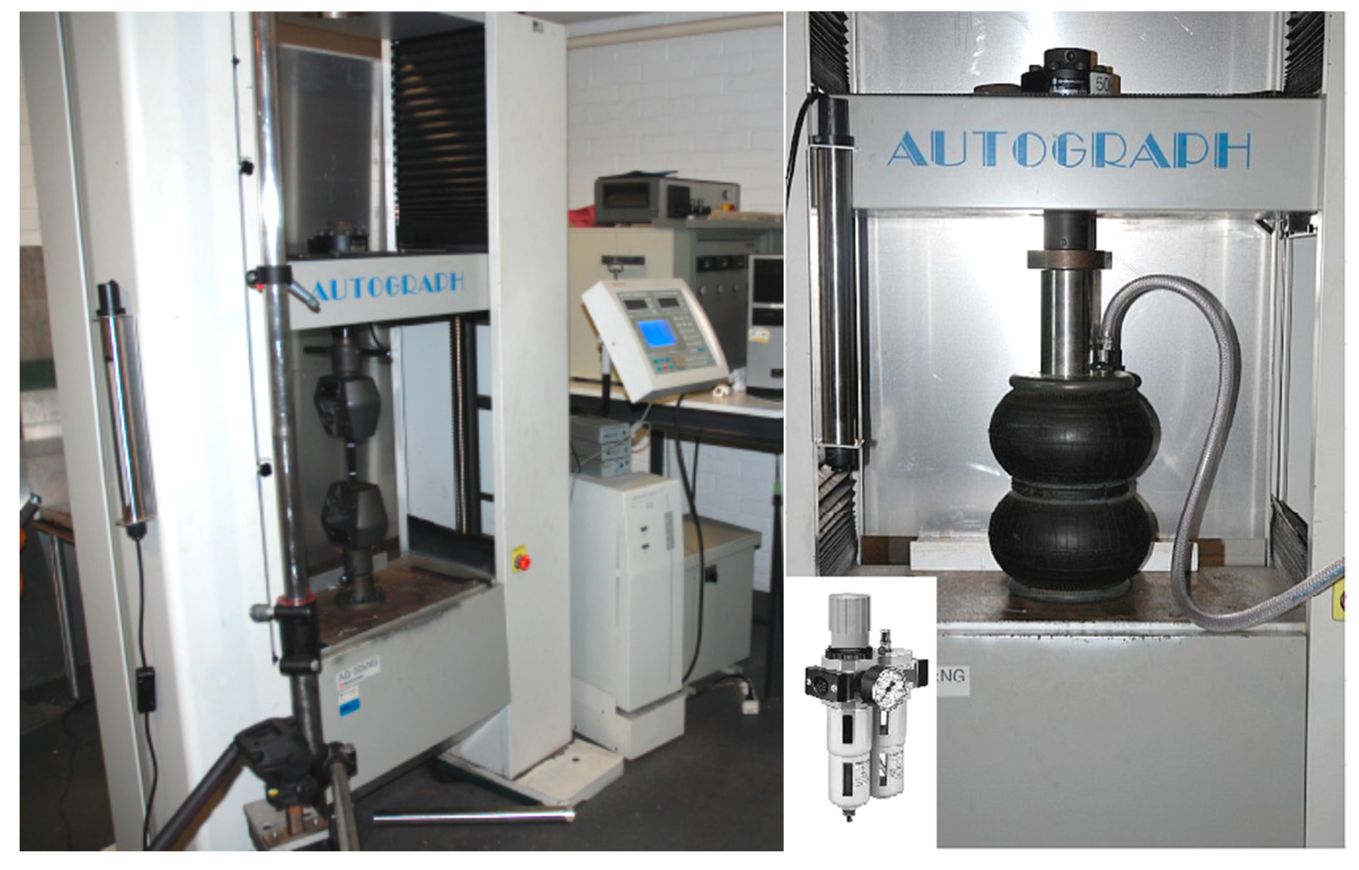
The experiment consisted of subjecting the bellows to a sequence of displacements in compression in a SHIMADZU-AUTOGRAPH® (from Kyoto, Japan) test machine (Figure 10) with 50 KN of capacity force. For safety reasons and to avoid exceeding the machine capacity, the spring displacement was restricted to an amplitude of 20 mm.
Given the likely sharp variation of the external loads acting in the structure of vehicle suspensions, it is plausible that the enclosed air spring undergoes adiabatic compressions. As the test is carried out at a very low speed, the internal air pressure has to be adjusted according to the thermodynamic law for a real (non-perfect) gas, at each time step. A pressure control unit was fitted in the pressure feed line to the bellows chamber (visible in Figure 10) to manually control the internal pressure at each time step of the test after having computed the internal volume at each step; naturally, the specimen is perfectly held in position during the pressure adjust. In a first step, the example was entirely solved with Newmark’s method to illustrate the main differences observed in relation to the linear systems in dynamic analysis. Only for testing the solution, an isothermal behavior was assumed, despite the dynamic characteristics of the problem. The pneumatic spring has a toroidal surround bellows and has the same overall dimensions and pneumatic parameters as the item analyzed in Section 2:
- Torus radius r = 50 mm
- Radius of circle passing through the transverse sections radius: R = 200 mm
- Initial pressure (preload pressure) P0 = 2 bar (≅0.2 MPa)
- External force F(t) = 10 KN (suddenly applied as a step load)
- Virtual mass of the SDOF system M = 50 Kg
The dynamic loading of the spring was approached with time steps Δt = 0.001 s (recommended time step less than Δtmax = 0.0066 s). The spring stiffness ranges from about Kmin = 191280 N/m (first time step) up to Kmax = 473911 N/m (time step for maximum displacement). It is noted that the spring stiffness here calculated refers to the effect of the axial displacement (equal to the double of the ovalization amplitude a) on the internal reaction force due to the air pressure as mentioned above:
Kmean = 332595 N/m.
For a suddenly applied load F = 10 KN, the dynamic spring stroke is:
Umax = 2 × Ustatic = 2 × (10,000/332,595) = 0.0601 m, which is a result close to the amplitude vibration calculated with the Newark algorithm as observed in the graphical results of Figure 11. The results show the accuracy of the method, where the amplitude of the vibrating system is double that of the static deflection. Also, the natural period T0 of this SDOF model (calculated with the averaged stiffness of the spring) is T0 = 0.077 s, which is also in good agreement with the numerical result in Figure 11.
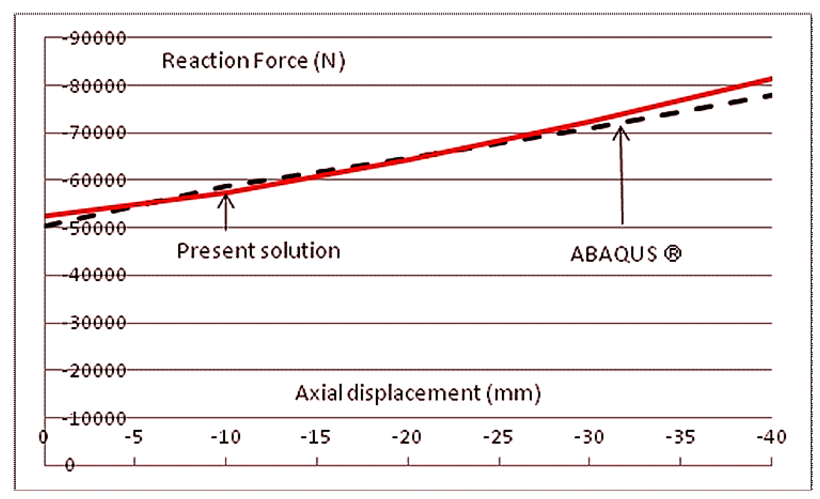
In Figure 10, the force response of the air spring versus the axial displacement is a slightly curved line, showing the expected non-linear behavior. This feature demands the use of iterative methods to predict the dynamic response of systems with these accessories, such as the one used here. Figure 12 shows the comparison of a test with a bellows spring similar to the previous test using the described solution and numerical modeling with ABAQUS® (SIMULIA-DASSAUL SYSTÈMES®—from Vélizy-Villacoublay, France). The compression was carried out in an isothermal regime with an initial pressure of 4 bars.
In the ABAQUS® simulation, the shell container was modeled using three-node quadratic axisymmetric shell elements (SAX2). Three integration points across the thickness were used for all of the layers i.e., the 0.40-mm thick outer rubber layers and the inner 0.20-mm thick steel layer. Rubber and steel were assumed to be elastic and isotropic with moduli equal to 0.1 GPa and 200 GPa, respectively. The Poisson’s ratios were 0.48 for the rubber and 0.30 for the steel. Geometrically non-linear analyses were conducted for the imposed internal pressure values. As observed, there is a good agreement of both results, despite a very small difference obtained with ABAQUS®.
3.4. Pseudo-Dynamic Test of a Real Pneumatic Spring: Procedures and Results
In this step, a pseudo-dynamic test of a commercial pneumatic spring, from Numatics® (Emerson Industrial Automation, www.numatics.com), is performed with the Shimadzu test machine, as shown in Figure 10. The double bellows tangent stiffness is calculated from the ratio of an incremental internal reaction Rt (measured with the load cell of the test machine) by the respective incremental relative displacement of both bellows flanges at each time step. The main problem data for the dynamic procedure were:
- A pneumatic double-bellows type spring (Numatics-Emerson®) having a rigid end flanges diameter of 160 mm. Internal pressure is p0 = 4 bar;
- A virtual mass M = 100 Kg (no damping considered);
- An impulsive step force F(t) = 1500 N sustained after instant t = 0+ s;
- No damping was considered in the dynamic model.
An estimation of this bellows stiffness gave an average value Kmean = 142,000 N/m. For the virtual mass M = 100 Kg, the natural period is T0 = 0.166 s.
The test was carried out by changing the internal air pressure according to the adiabatic equation: , where γ is the adiabatic exponent, here assumed to be about 1.3 (an adequate value for real gases) and an initial internal volume of the accessory V0 ≅ 6.2 l (0.0062 m3). The dynamic response for this SDOF system was obtained with a total Newmark’s non-linear solution, where the spring tangent stiffness was calculated at each time step upon changing the internal pressure according to the adiabatic equation.
The same problem was simulated with a pseudo-dynamic procedure, where the system stiffness at each time step was calculated by the rate of the spring internal force (measured with the machine load cell) versus each displacement increment obtained with precision linear voltage displacement transducers (LVDTs with a resolution of up to 5 μm) fitted in the machine. As the equipment was not automated for this pseudo-dynamic procedure, the air pressure was manually adjusted in the compressed air distribution unit after obtaining the internal volume for each axial displacement of the spring (available in technical information by the manufacturer), and then substituting its value in the adiabatic equation that was solved for the internal pressure at the spring displacement at time step t. Results for the pseudo-dynamic procedure are depicted in Figure 13, where a good agreement of both methods is observed, despite the slight mismatch among the natural periods estimated with the methods.
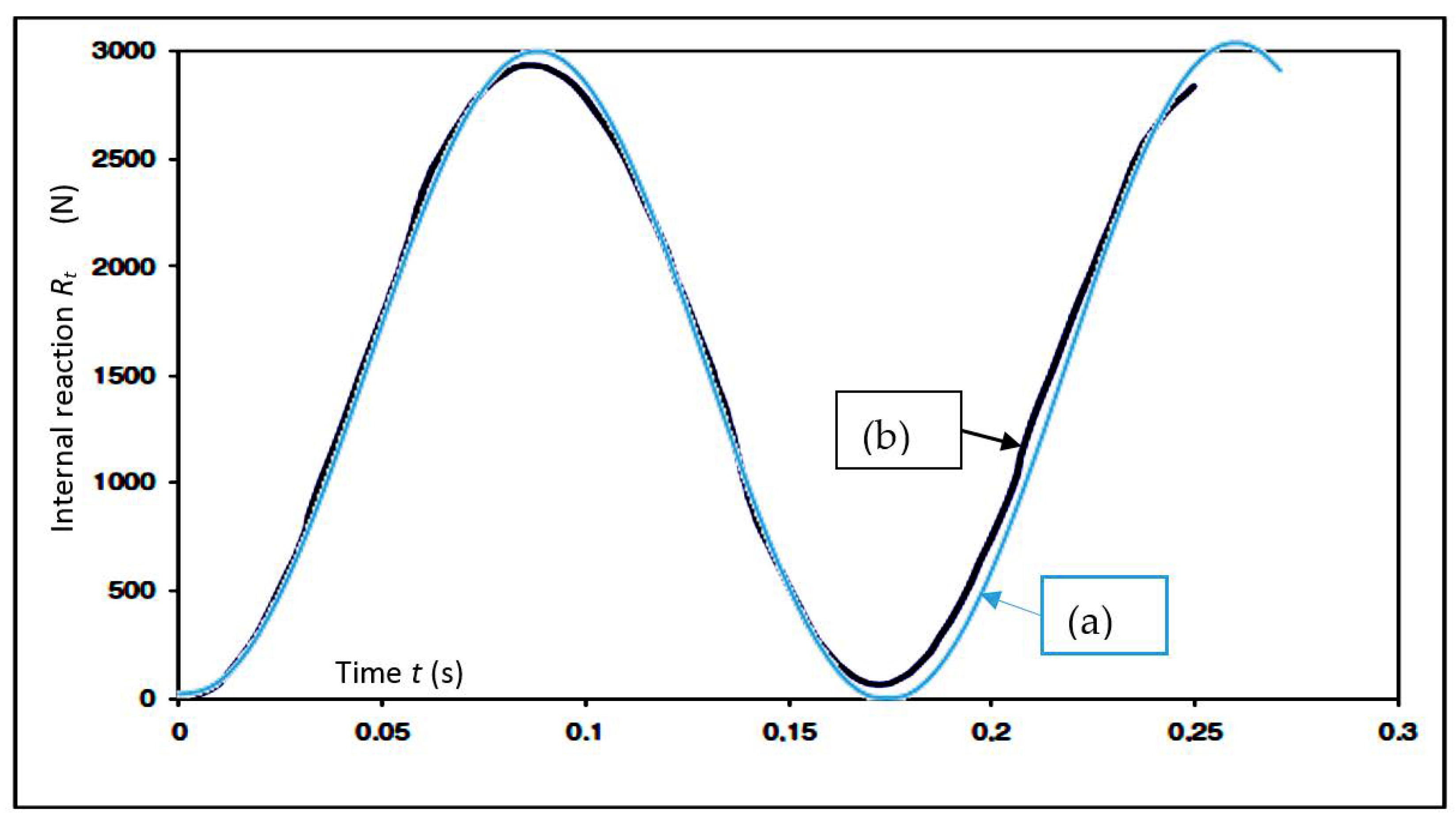
The peak axial displacement obtained with the pseudo-dynamic procedure at maximum reaction force (3000 N) was about 18 mm, while a simple calculation for a linear system (with spring stiffness Kmean = 142,000 N/m) showed that 21 mm was the maximum value. Although acceptably close, repeated cycles (with the pseudo-dynamic procedure) revealed a progressive degradation of the agreement between the experimental and theoretical results.
4. Conclusions
Conclusions may be drawn from the work here presented on the stiffness of bellows-type air springs used in automotive suspension:
- A simple yet accurate shell model was developed by variational techniques based on the minimum deformation energy concept and essential thermodynamics of gases. For enhanced accuracy, the influence of the velocity of the deformation was included by selecting isothermal or adiabatic compression regimes for the air suspension.
- The present model predictions agreed very well with a finite element model constructed in a commercial code with axisymmetric high order shell finite elements.
The pseudo-dynamic method proved to be a useful alternative to dynamical testing equipment, not only for its accuracy, but also for the cheaper rig and instrumentation. Furthermore, this method was able to deal with the non-linear behavior in a very effective manner, given the one-degree of freedom nature of the system here analyzed. Naturally, important limitations arise when a precise deformation of the structure can be achieved only with a large number of degrees of freedom of displacement and rotation modes.
Author Contributions
Conceptualization, F.J.M.Q.d.M.; Investigation, F.J.M.Q.d.M., A.B.P. and A.B.M.; Software, A.B.M.; Supervision, F.J.M.Q.d.M.; Validation, A.B.P.; Writing—original draft, F.J.M.Q.d.M.; Writing—review & editing, A.B.P.
Funding
This work obtained financial support from projects UID/EMS/00481/2013-FCT and CENTRO-01-0145-FEDER-022083.
Conflicts of Interest
The authors declare no conflict of interest. The founding sponsors had no role in the design of the study; in the collection, analyses, or interpretation of data; in the writing of the manuscript, and in the decision to publish the results.
References
- Humphreys, W. Pneumatic Spring for Vehicles. U.S. Patent 673,682, 22 January 1901. [Google Scholar]
- Sainsbury, H. Air Suspension for Road Vehicles. Proc. Inst. Mech. Eng. Automob. Div. 1957, 11, 75–101. [Google Scholar] [CrossRef]
- Quaglia, J.; Sorli, M. Air Suspension Dimensionless Analysis and Design Procedure. Veh. Syst. Dyn. 2010, 35, 443–475. [Google Scholar] [CrossRef]
- Löcken, F.; Welsch, M. The Dynamic Characteristic and Hysteresis Effect of an Air Spring. Int. J. Appl. Mech. Eng. 2015, 20, 127–145. [Google Scholar] [CrossRef] [Green Version]
- Zhang, Y.; Huang, H.; Chen, R.; He, M. Studies on Modeling a Single-Bellows Air Spring and Simulating its Inherent Characteristics. In Proceedings of the 5th International Conference on Information Engineering for Mechanics and Materials, Huhhot, China, 25–26 July 2015. [Google Scholar] [CrossRef]
- Apostol, M. Calculus Volume II, 2nd ed.; John Wiley & Sons: New York, NY, USA, 1969; pp. 312–323. ISBN 0-471-00007-8. [Google Scholar]
- Ugural, A. Stresses in Plates and Shells, 2nd ed.; McGraw-Hill Co.: New York, NY, USA, 1999; pp. 211–236. ISBN 0070657696. [Google Scholar]
- Reddy, J. An Introduction to Non-Linear Finite Element Analysis, 2nd ed.; Oxford University Press: New York, NY, USA, 2004; pp. 430–447. ISBN 9780199641758. [Google Scholar]
- Newmark, M. A method of computation for structural dynamics. ASCE J. Eng. Mech. Div. 1959, 85, 67–94. [Google Scholar]
- Pinto, A.; Verzeletti, G.; Molina, J.; Varum, H.; Pinho, R.; Coelho, E. Pseudo-Dynamic Tests of Non-Seismic Resisting RC Frames (Bare and Selective Retrofit Frames); JRC-EUR 20244 EN Report; Joint Research Centre: Ispra, Italy, 2002. [Google Scholar]
- Pinto, A.; Pegon, P.; Magonette, G.; Tsionis, G. Pseudo-dynamic testing of bridges using non-linear substructuring, Earthquake Engineering Structural Dynamics. J. Int. Assoc. Earthq. Eng. 2004, 33, 1125–1186. [Google Scholar] [CrossRef]
- Carneiro, J.; Melo, F.; Pereira, J.; Teixeira, V. Pseudo-Dynamic Method for Structural Analysis of Automobile Seats. Proc. Inst. Mech. Eng. Part K J. Multi-Body Dyn. 2005, 219, 337–344. [Google Scholar] [CrossRef] [Green Version]
- Malmedahl, G. Analysis of Automotive Damper Data and Design of a Portable Measurement System. Bachelor’s Thesis, Department of Mechanical Engineering, Center for Automotive Research, The Ohio State University, Columbus, OH, USA, December 2005. [Google Scholar] [Green Version]
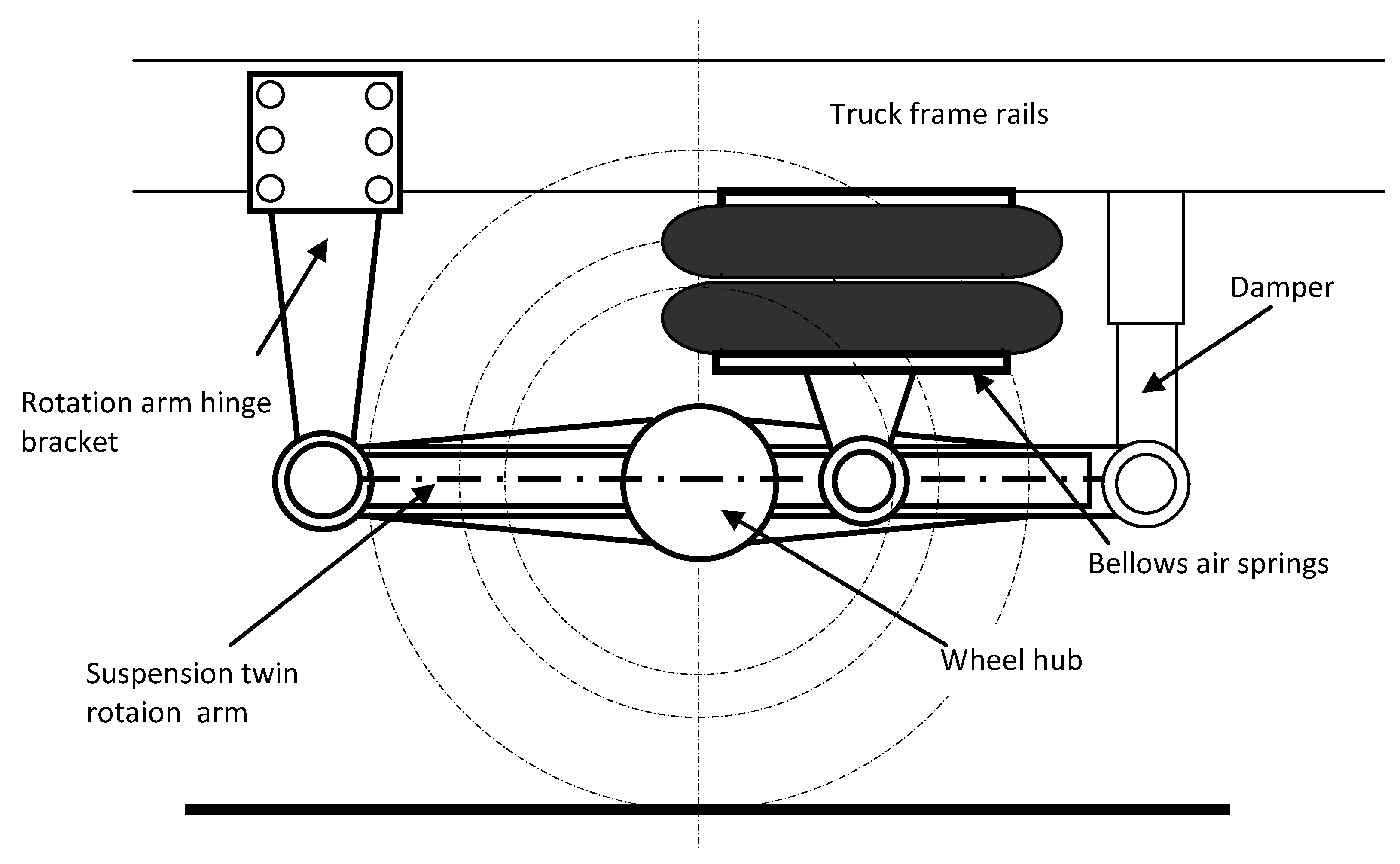
Figure 1.
An example of a solution design of a rear air spring truck or trailer suspension.

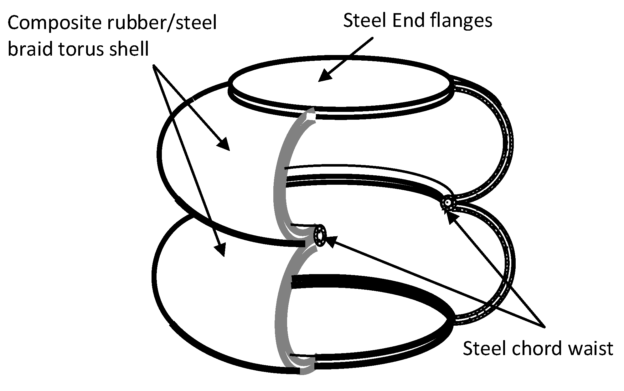
Figure 2.
Double cell bellows air spring.

Figure 3.
Axisymmetric toroidal shell element under internal pressure: displacement field by axial loads.
Figure 3.
Axisymmetric toroidal shell element under internal pressure: displacement field by axial loads.

Figure 4.
Scheme of the iterative procedure with the Newton–Raphson method.

Figure 5.
Internal reaction vs axial displacement (in compression) of the pneumatic spring with isothermal and adiabatic (γ = 1.3) processes. Initial internal pressure p0 = 2 bar (displacements indicated are half of each prescribed spring stroke for symmetry).
Figure 5.
Internal reaction vs axial displacement (in compression) of the pneumatic spring with isothermal and adiabatic (γ = 1.3) processes. Initial internal pressure p0 = 2 bar (displacements indicated are half of each prescribed spring stroke for symmetry).
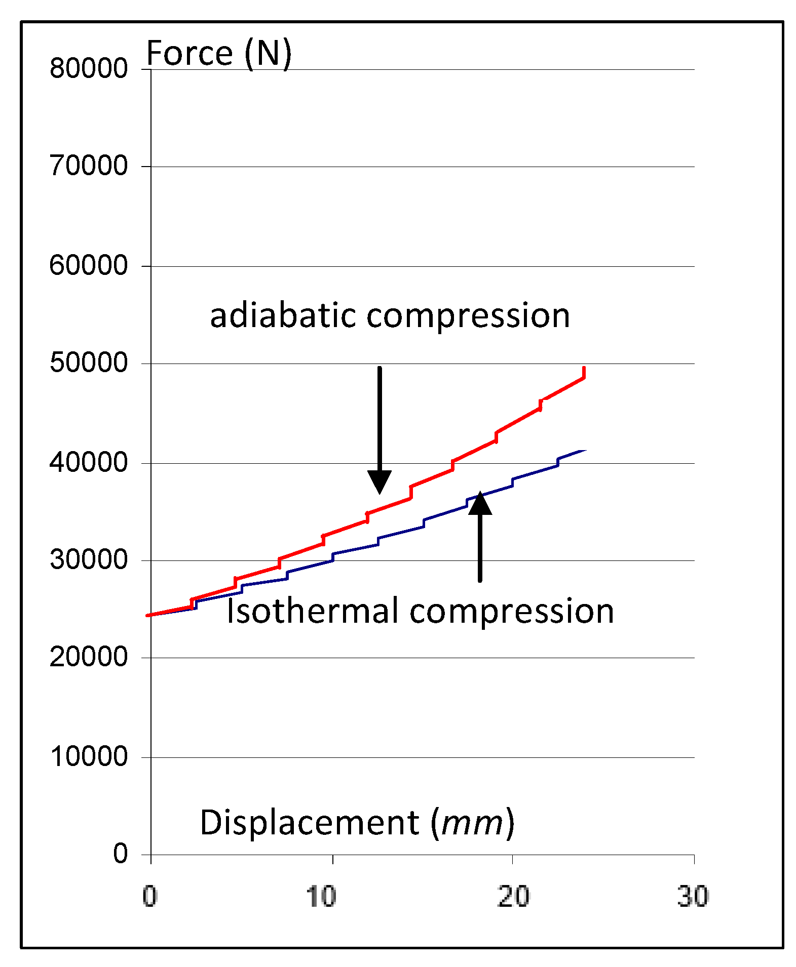
Figure 6.
Sketch of a vehicle suspension and the equivalent dynamic model for a case of passive transmission: (a) drawing; and (b) symbology.
Figure 6.
Sketch of a vehicle suspension and the equivalent dynamic model for a case of passive transmission: (a) drawing; and (b) symbology.
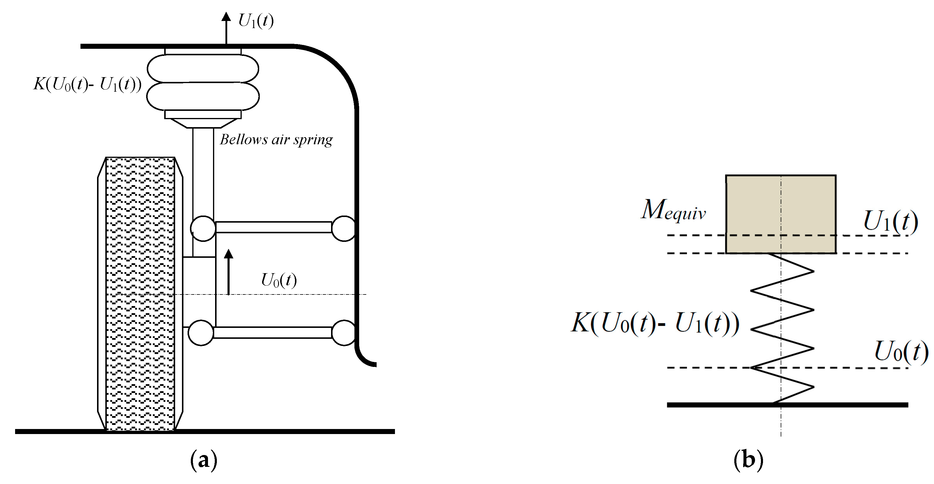
Figure 7.
Operation diagram of a closed-loop pseudo-dynamic procedure.

Figure 8.
Pseudo-dynamic test rig for structural validation of bus passenger seats (figure not included in the work of Pinto et al. [12]).
Figure 8.
Pseudo-dynamic test rig for structural validation of bus passenger seats (figure not included in the work of Pinto et al. [12]).
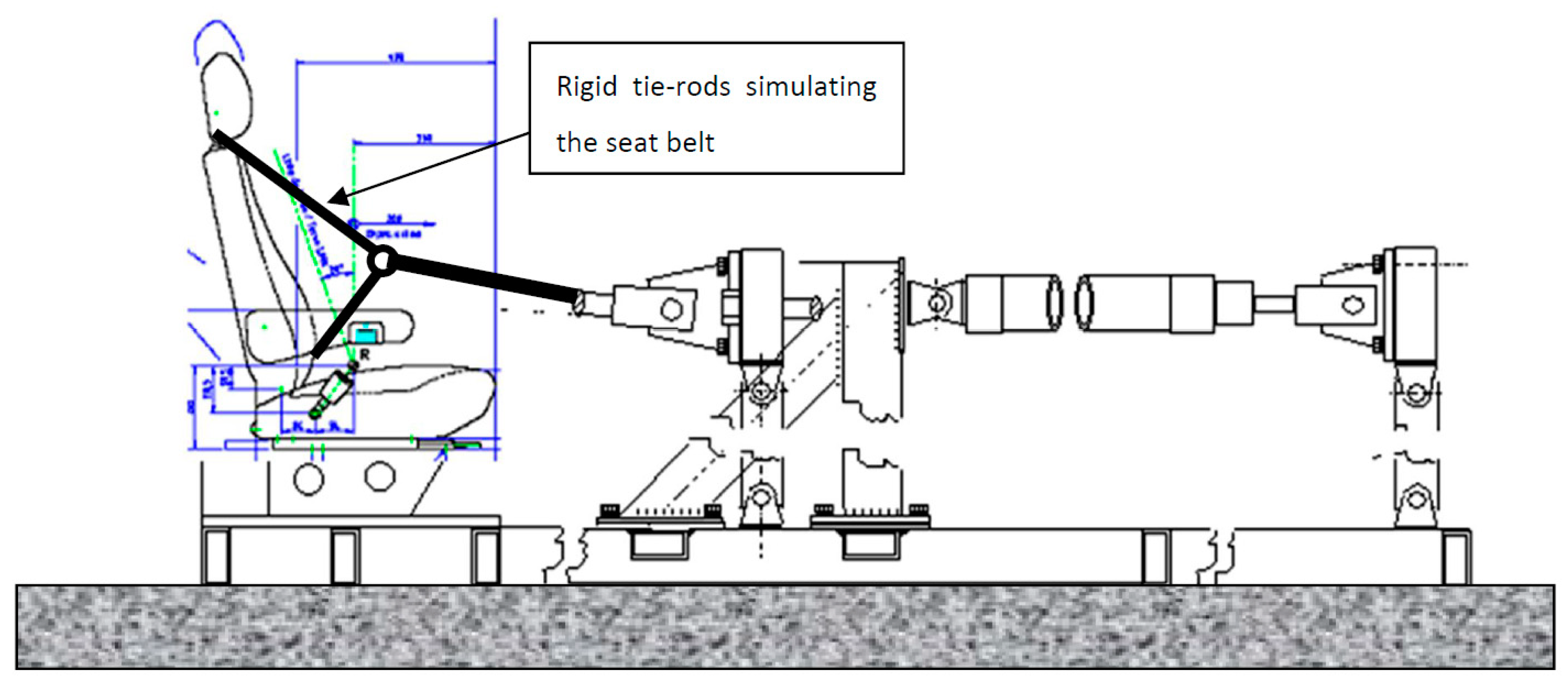
Figure 9.
Acceleration at the wheel of a vehicle tire and suspension set hitting the soil suddenly from a small height. Points were collected from Malmedahl [13] having shifted them of about 0.1 s so that the starting point could match approximately the corresponding results here evaluated.
Figure 9.
Acceleration at the wheel of a vehicle tire and suspension set hitting the soil suddenly from a small height. Points were collected from Malmedahl [13] having shifted them of about 0.1 s so that the starting point could match approximately the corresponding results here evaluated.

Figure 10.
Mounting of the bellows pneumatic accessory in a SHIMADZU® testing machine between the working table and upper crosshead with an adaptor ram and a pressure air control unit.
Figure 10.
Mounting of the bellows pneumatic accessory in a SHIMADZU® testing machine between the working table and upper crosshead with an adaptor ram and a pressure air control unit.

Figure 11.
Internal reaction versus axial displacement of the pneumatic spring analyzed. (a) Displacement versus time after application of an impulsive step load F0 = 10 KN; (b) Force/displacement relation of the pneumatic spring.
Figure 11.
Internal reaction versus axial displacement of the pneumatic spring analyzed. (a) Displacement versus time after application of an impulsive step load F0 = 10 KN; (b) Force/displacement relation of the pneumatic spring.
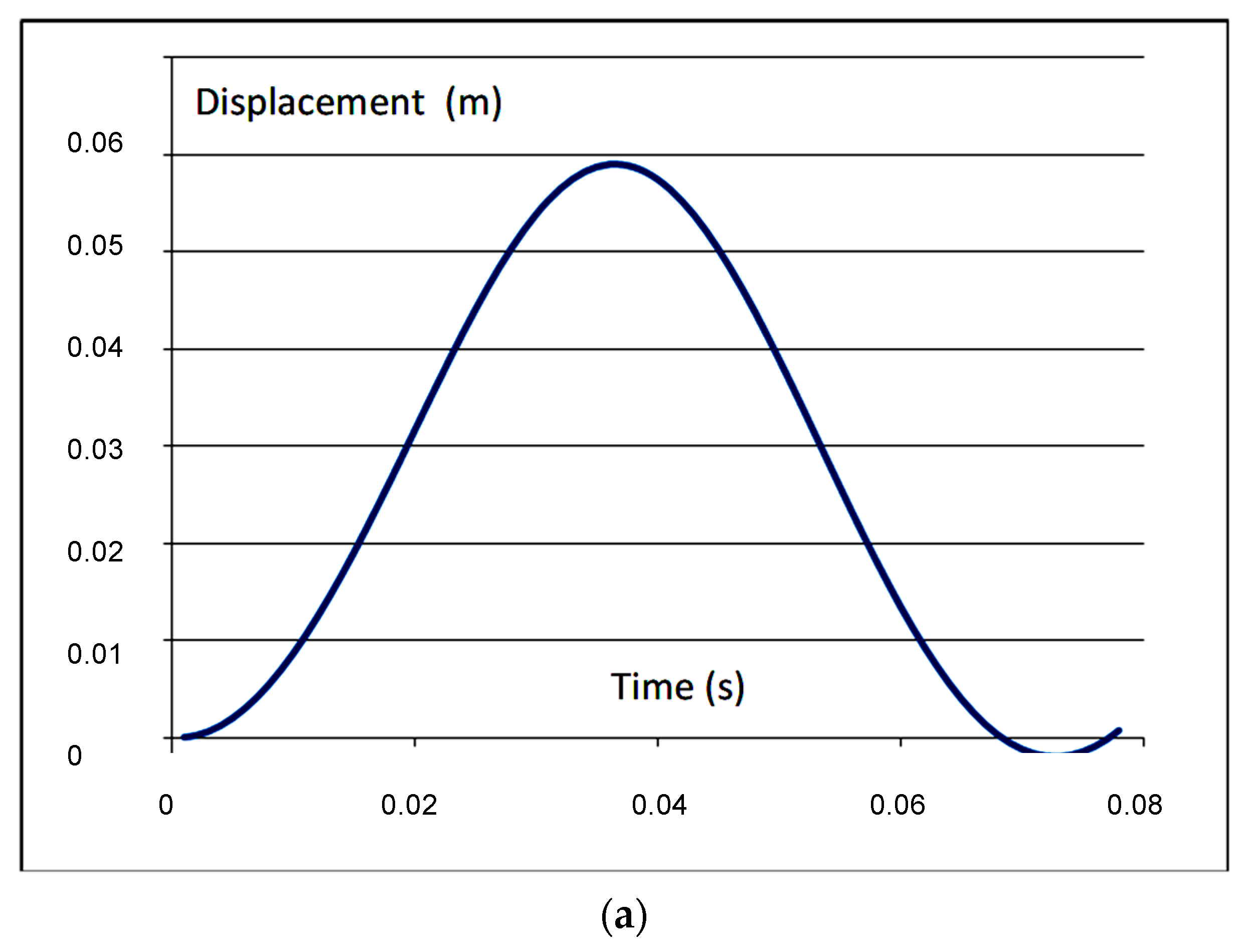
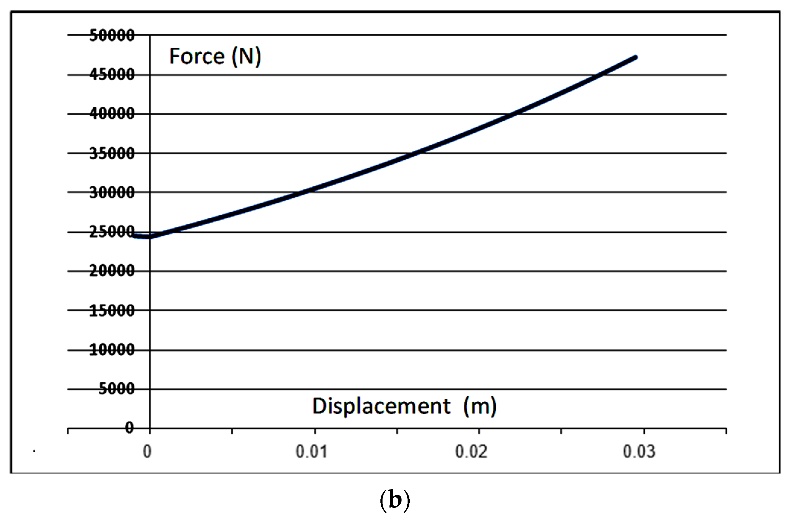
Figure 12.
Spring response from prescribed axial displacements with the presented method and ABAQUS® (Axisymmetric shell elements with ABAQUS®, with geometry similar to the previous example but initial pressure = 4 bar).
Figure 12.
Spring response from prescribed axial displacements with the presented method and ABAQUS® (Axisymmetric shell elements with ABAQUS®, with geometry similar to the previous example but initial pressure = 4 bar).

Figure 13.
Results for the vibration of a single degree of freedom (SDOF) system with the pneumatic spring in analysis: (a) with Newmark’s method (natural period is ≅0.180 s); and (b) with a pseudo-dynamic simulation (natural period is ≅0.175 s).
Figure 13.
Results for the vibration of a single degree of freedom (SDOF) system with the pneumatic spring in analysis: (a) with Newmark’s method (natural period is ≅0.180 s); and (b) with a pseudo-dynamic simulation (natural period is ≅0.175 s).

© 2018 by the authors. Licensee MDPI, Basel, Switzerland. This article is an open access article distributed under the terms and conditions of the Creative Commons Attribution (CC BY) license (http://creativecommons.org/licenses/by/4.0/).
Share and Cite
MDPI and ACS Style
De Melo, F.J.M.Q.; Pereira, A.B.; Morais, A.B. The Simulation of an Automotive Air Spring Suspension Using a Pseudo-Dynamic Procedure. Appl. Sci. 2018, 8, 1049. https://doi.org/10.3390/app8071049
AMA Style
De Melo FJMQ, Pereira AB, Morais AB. The Simulation of an Automotive Air Spring Suspension Using a Pseudo-Dynamic Procedure. Applied Sciences. 2018; 8(7):1049. https://doi.org/10.3390/app8071049
Chicago/Turabian StyleDe Melo, Francisco J. M. Q., António B. Pereira, and Alfredo B. Morais. 2018. "The Simulation of an Automotive Air Spring Suspension Using a Pseudo-Dynamic Procedure" Applied Sciences 8, no. 7: 1049. https://doi.org/10.3390/app8071049
Note that from the first issue of 2016, this journal uses article numbers instead of page numbers. See further details here.