Fault Location in Double Circuit Medium Power Distribution Networks Using an Impedance-Based Method


1
Department of Electrical Engineering, Persian Gulf University, Bushehr 7516913817, Iran
2
Bushehr Province Electricity Power Distribution Company, Bushehr 7515784311, Iran
3
Center for Energy Informatics, University of Southern Denmark, 5230 Odense, Denmark
*
Author to whom correspondence should be addressed.
Appl. Sci. 2018, 8(7), 1034; https://doi.org/10.3390/app8071034
Submission received: 31 May 2018
/
Revised: 18 June 2018
/
Accepted: 20 June 2018
/
Published: 25 June 2018
(This article belongs to the Special Issue Distribution Power Systems)
Abstract
:The distribution network is extended throughout cities, towns, and villages. Because of the increase in loads and the decrease in power passageways and public corridor reduction, double circuit lines are increasingly being used instead of single circuit lines. Fault location in double circuit power networks is very important because it decreases the repair time and consequently the power outage time. In this paper, a new improved method for fault location in double circuit medium power distribution lines is proposed. The suggested impedance-based fault location method takes into account the mutual effect of double circuit lines on each other. To the best of our knowledge, the proposed method is the first of its kind which supports double circuit distribution networks. In the proposed method, a new quadratic equation for locating fault in power distribution networks is obtained using recorded voltage and current at the beginning of feeder. In this method, the π line model is used for improving the accuracy of the suggested method. The proposed method is supported by mathematical proofs and derivation. To evaluate the accuracy of the proposed method, the proposed method is tested on a thirteen-node network in different conditions, such as instrument error, various fault resistances, and different fault inception angles in various distances and fault types. The numerical results confirm the high accuracy and validity of the proposed method.
1. Introduction
1.1. Motivation
Distribution networks are important because of their interesting properties and conditions, such as span, dispersion, unbalanced loads, and non-homogeneity. They are also important because they are the last point of power delivery to consumers. Distribution networks are vulnerable to different faults which affect the system’s reliability, security, and quality. Therefore, maintaining system stability, minimizing interrupted consumers and damaged networks as quickly as possible are very important. Therefore, fault location techniques play a vital role in repairing and fixing system faults in the least amount of time possible [1,2,3,4,5,6,7,8,9,10,11,12,13,14].
All of the fault location methods which have been presented so far have been developed for single circuit distribution networks, and double circuit networks have unfortunately not been addressed. Past studies on fault location have usually used a short line model and neglected the effect of capacitors. However, recent papers have used more complete models, such as the medium line model (π) or the widespread line model for fault location. Needless to say, they only address single circuit lines and not double circuit lines. In double circuit lines, the mutual effects of the lines on each other and power outages are greater than single circuit lines. Because of the high amount of consumers, if power outage occurs on the lines there will be a vast amount of undistributed power (energy). Most of the double circuit lines are overhead cables with no insulator.
If a power outage occurs somewhere along the power lines, it must be considered that the fault could be in either of the adjacent lines. Thus, locating faults in double circuit lines is more complicated than in single lines. Because of the complexity and specific conditional and operational features, fault location in double circuit lines remains a challenge to this day.
1.2. Literature Review and Challenges
Since 1980, fault location algorithms have seen substantial development, particularly methods that are based on impedance. At the beginning of these developments, power systems were modeled based on symmetric geometric lines and analyzed based on symmetric parts which were specifically used for underground systems (e.g., the method used in [1,2]). Reference [3] uses symmetric factors based on the line’s parallel admittance which is also used only for underground distribution networks. In [4], the accuracy was improved significantly by considering the effect of capacitors. However, this can only be used for underground systems. In [5], a method was proposed for determining the distance to a single-phase fault in overhead distribution cables based on the base frequency, voltage, and current at the beginning of the feeder. In this method, by using the short line model and series and parallel analysis, the impedance of different routes were evaluated. Salim [6] proposed a new method for fault location by considering a π line model. This method uses the corrected impedance, and a quadratic equation in accordance with the fault distance is obtained. By using this method, the fault detection accuracy was improved and maximum error percentage was reported to be 1.58%. In [7], a new and precise fault location algorithm was provided by considering the effect of capacitors. This method has a higher accuracy than previous methods. The downside of this method is that it can only be used for single circuit distribution networks.
In [8], special attention was given to the dynamic model. In this work, the fault distance was estimated through the load amount. The load amount was calculated from the load factor and power factor. In [9], a method was given to determine the specific fault location since there might be more than one fault in the system. As a result, two approaches were used to determine the real fault’s location. The first approach compares the measured and recorded voltage samples, and the second approach uses the voltage’s frequency spectrum.
A hybrid fault location method is presented for single line to ground fault in [15]. At first, the possible fault locations are determined using an impedance-based fault location method. Then, the faulty section or the main fault location among the determined possible fault locations is strongminded using a voltage sag matching algorithm. In [16], the fault location in the four-wire lines is determined by improving the algorithm presented in [15].
A time domain technique is presented for locating faults in a power distribution network (PDN) [17]. It uses the voltage and current at the beginning of the feeder and distributed generator DG place. Furthermore, an iterative method is presented to solve the fault location problem. The need for a high sampling rate is the drawback of this method.
The self-healing concept is used for locating faults in PDN with DG in [18]. In this paper, the fault location algorithm requires the transient and steady state of signals, load flow algorithm, and synchronization angle.
Furthermore, the important papers in this topic are reviewed and the characteristics and details are shown in Table 1.
1.3. Approach and Contributions
In this paper, an improved impedance-based method is proposed for fault location in double circuit power distribution networks. In the suggested method, a collection of equations are derived to prove a new quadratic equation for locating fault in double circuit lines. The method is applied using only the recorded voltage and current at the beginning of the feeder. In this method, after distinguishing the short circuit fault, the voltage and current of each section of the distribution network is calculated through Kirchhoff’s voltage law KVL and Kirchhoff’s current law (KCL) equations, and the location of the fault is determined using the proposed method. In the proposed method, the capacitor effect and the mutual effect of the lines on each other is considered. The suggested method is tested in a thirteen-node system using MATLAB simulation and the results confirm the method’s accuracy and validity. The obtained results show that the accuracy of the proposed method is very high and the sensitivity is very low in different fault conditions.
1.4. Paper Organization
2. The Proposed Method
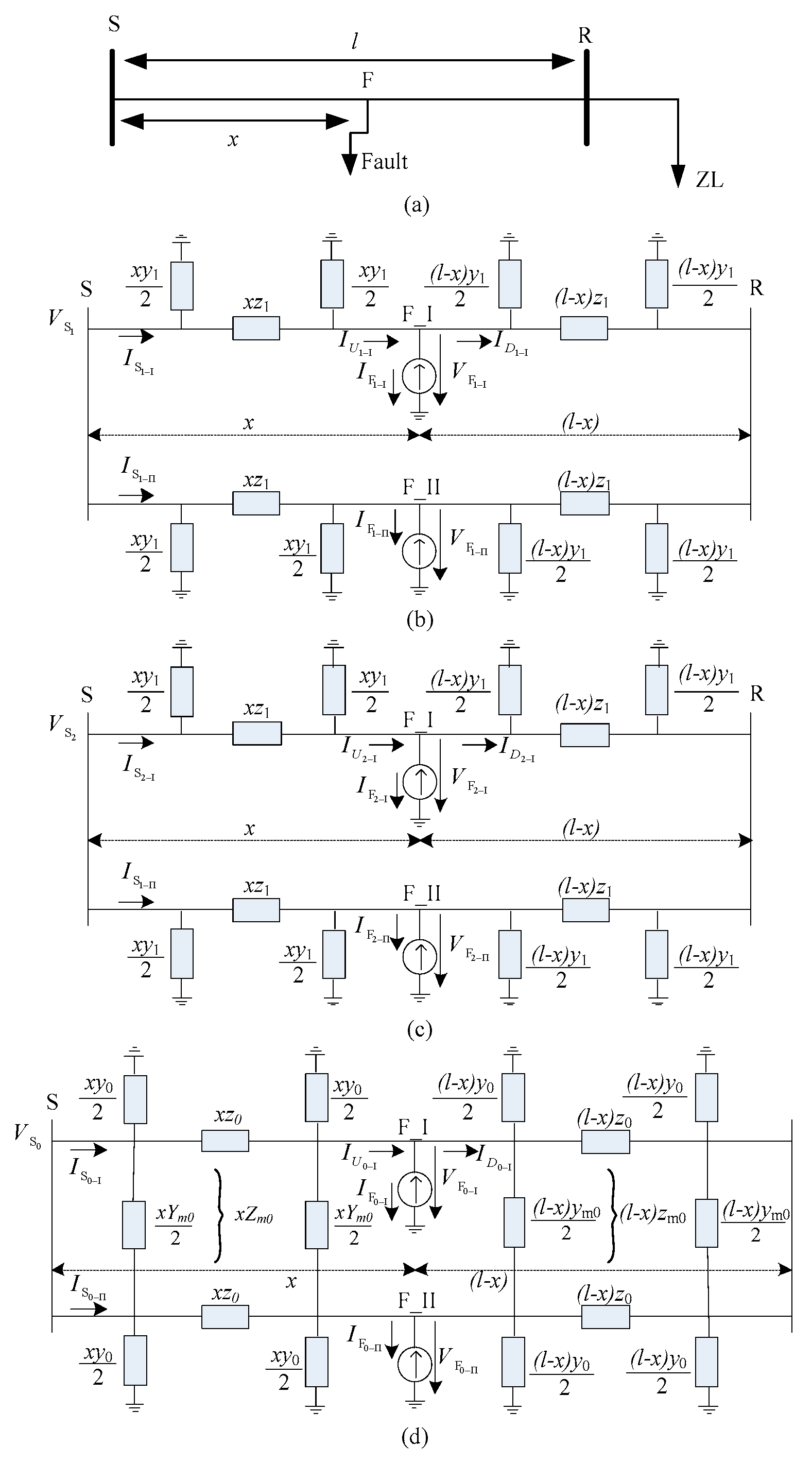
The distribution network consists of different parts. In this article, the line is considered as the part between two buses. By using a π line model, Figure 1 shows a single-line diagram of each section for the positive, negative, and zero sequences of a double circuit network for a normal fault in point .
Notations in Figure 1 are as follows:
According to Figure 1b–d and by defining by (1) to simplify by (3), positive, negative, and zero sequence voltages in fault point are obtained, and by using Fortescue’s transformation matrix (by (2)) as (abc) by (3) is produced:
Now, by defining E, G, H, and L, can be obtained from Equation (5):
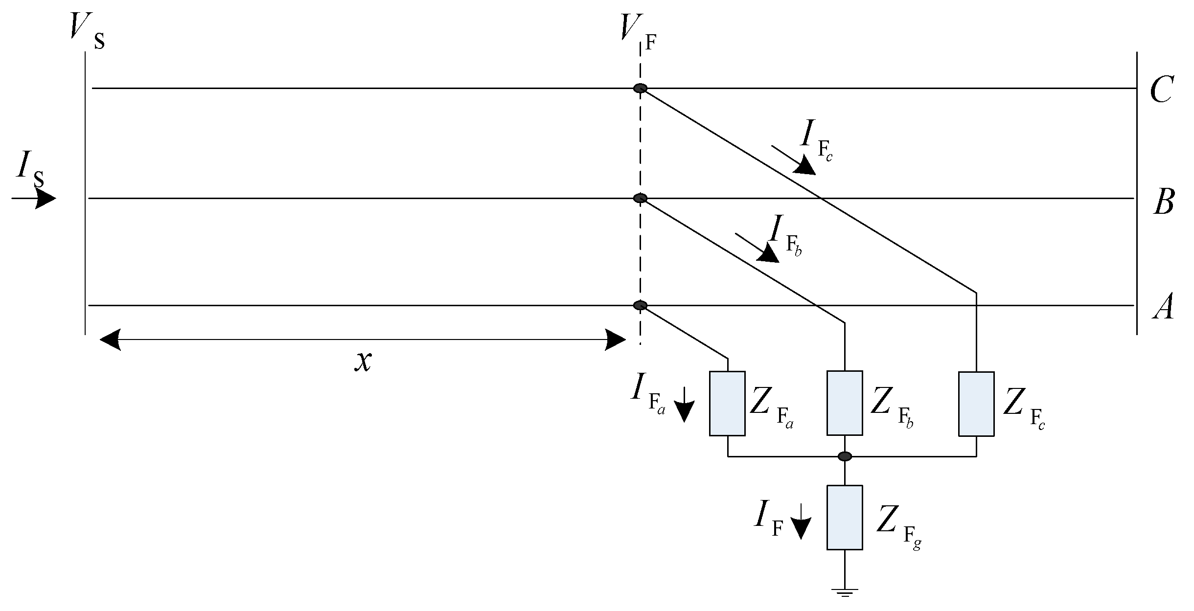
The most general fault model is shown in Figure 2, which models faults such as single phase to the ground, two phases to the ground, and three phases to the ground. In this section, a quadratic equation is suggested, and it is proven that it can determine the distance of ground faults with a suitable accuracy. By using the equation below, the voltage at the point of the fault is calculated:
where a, b, and c are the phases of the faults impedance , as shown in Figure 2. The above equation is only suitable for fault phases that have a current not equal to zero. By inserting Equation (6) in to Equation (5) for each k-phase, we will have:
where is the impedance and is the current of the k-phase.
As shown in Figure 2, is the fault’s current. Considering the fault’s impedance as a pure resistance and by separating Equation (7) into two parts (real and imaginary), Equation (8) is obtained:
In the above equation, index r indicates the real part and index i indicates the imaginary part of these variables. Equation (8) can be used for equation matching and to separate the fault resistance from each faulted phase; thus, a group of n equations are obtained which are independent of and dependent on x, , and .
By multiplying to Equation (9) and completing the algebraic calculations, the below equation is obtained:
In this equation, shows the real part, shows the imaginary part, and indicates the conjugate of the complex numbers. For each k-phase, Equation (10) can be re-written:
Based on the equation below
and if we consider as the fault’s resistance, the next equation is derived:
where is a group of faulted phases that consist of the system’s (a), (b), and (c) phases. In a three-phase system, there are seven different states of faults, including single-phase, two-phase, and three-phase. By replacing Equation (8) into Equation (12) and by making the algebraic changes in the mentioned equation, the final fault location equation for ground-faults, named the general ground-fault equation, is obtained:
It is important to mention that this is a fault location equation, and it is used for determining the fault distance. Therefore, it needs the three-phase voltage and current in the post, line parameters (series impedance and parallel admittance), and the faults current (because the fault current cannot be determined in local station, Equation (4) is used to calculate the coefficients of Equation (13)). As a result, an equation is needed to estimate the fault current, which will be provided in Section 3.
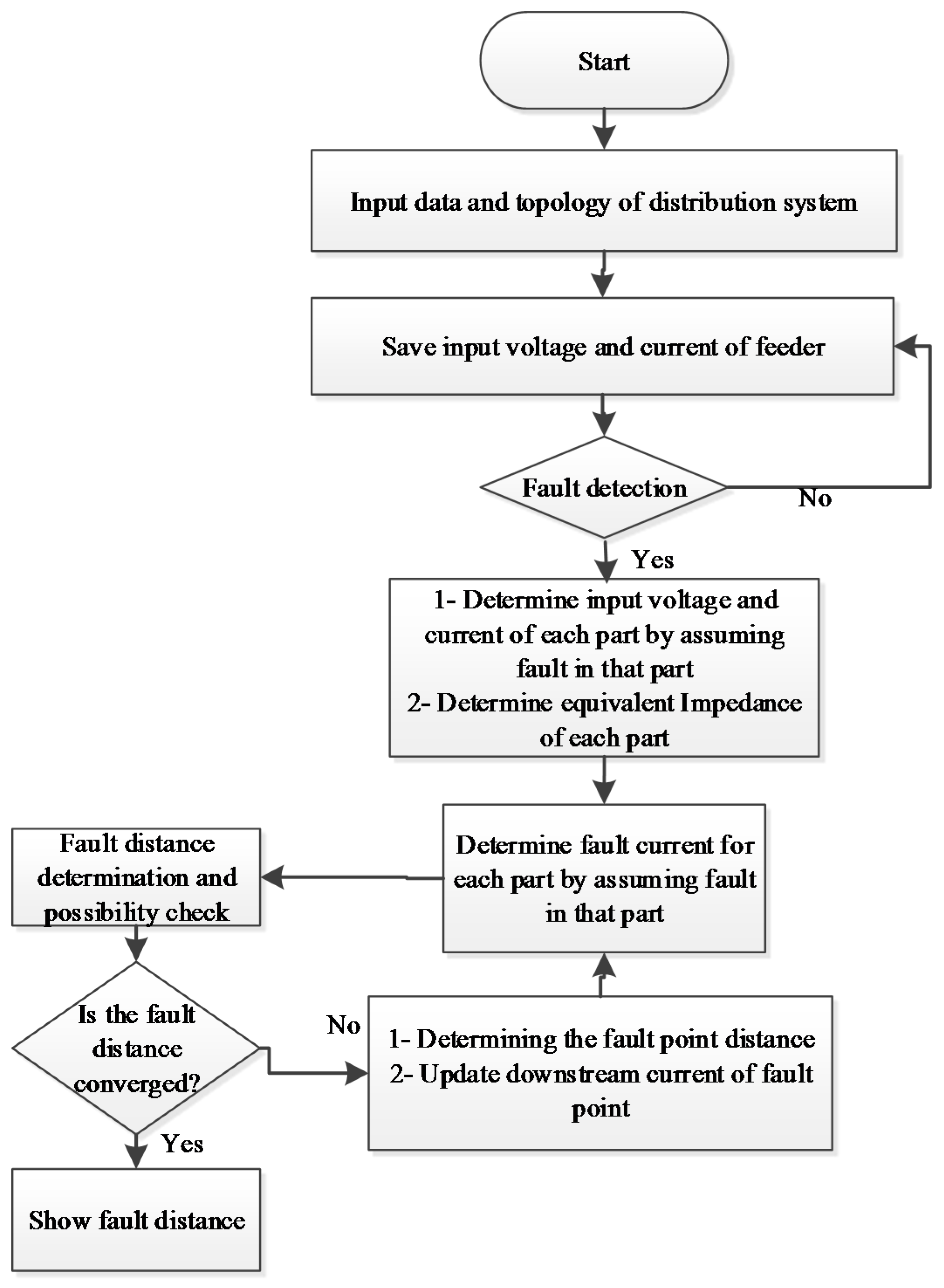
3. The Developed Fault Location Algorithm
The developed method in this paper considers the mutual effects of the lines on each other. It also considers the existence of central loads and the main and subsidiary branches for a double circuit. The details of the algorithm are given below:
- (1)
- Fault detection.
- (2)
- Determining the fault type.
- (3)
- Estimation of the fault current using the equation below:where and are the measured currents during and before the fault in the local relay.
- (4)
- Determining the fault’s distance from the general fault location equation (Equation (13)).
- (5)
- Determining the exact physical location of the fault.
- (6)
- Checking the convergence of using Equation (15):For > 1, the tolerance δ is predefined and n is the number of repetitions.
- (7)
- If is convergent with the analyzed part of the last section, then is the fault’s location and go to the next step; if it is convergent with a location beyond the current location, then we update and in the system’s next bus (changing the reference bus) and return to section one.
- (8)
- Calculating the fault’s point voltage by using Equation (5), , voltages and currents of the bus in the correct analyzed upstream section (k in and refers to the reference bus).
- (9)
- Updating the fault’s downstream current in the faulted phases using the calculated voltage of the fault point and based on Equation (16), finally is obtained using Fortescue’s conversion as seen in Equation (20).In the above equation, in series state one and two, is obtained from Equation (17), in which is the impedance connected to the -bus. Additionally, for obtaining the equivalent impedance in zero series state, Equations (18) and (19) are obtained from Y-Δ and Δ-Y conversions, and finally is derived:
- (10)
- Updating the faults current by using Equation (21):where is the upstream current of the faulted point according to Figure 1.is obtained using Fortescue’s conversion.
- (11)
- Return to step four.
It is known that the distribution feeders are distributed in single circuit or double circuit. This depends upon the load demands and its peak. These loads can be unbalanced and distributed in the feeder. Therefore, in the proposed method, the KVL and KCL matrices are used. The symmetrical components are taken into account in the proposed method just for calculating the updated downstream current in the faulty section. From Equations (3), (6) and (13), it can be seen that the unbalanced feeder can be analyzed because its effect on the current and voltage is known. Furthermore, in practice, the phases voltage and current can be obtained from the Over Current/Earth Fault and Over/Under Voltage relay which is installed at the beginning of the feeder.
Determining a Physical Solution
The proposed equations for fault location are second-order polynomial equations in terms of x, where x represents the fault’s distance. As a result, two new distances for the fault are obtained for each iteration of the explained algorithm. One of them is a positive and is coordinated with the section under evaluation, and the other one is purely mathematical and has no physical meaning.
The fault’s distance x is obtained from the following equations, which show the correct physical solution:
The flowchart of the proposed method is shown in Figure 3.
4. Simulation Results
4.1. The Studied Network
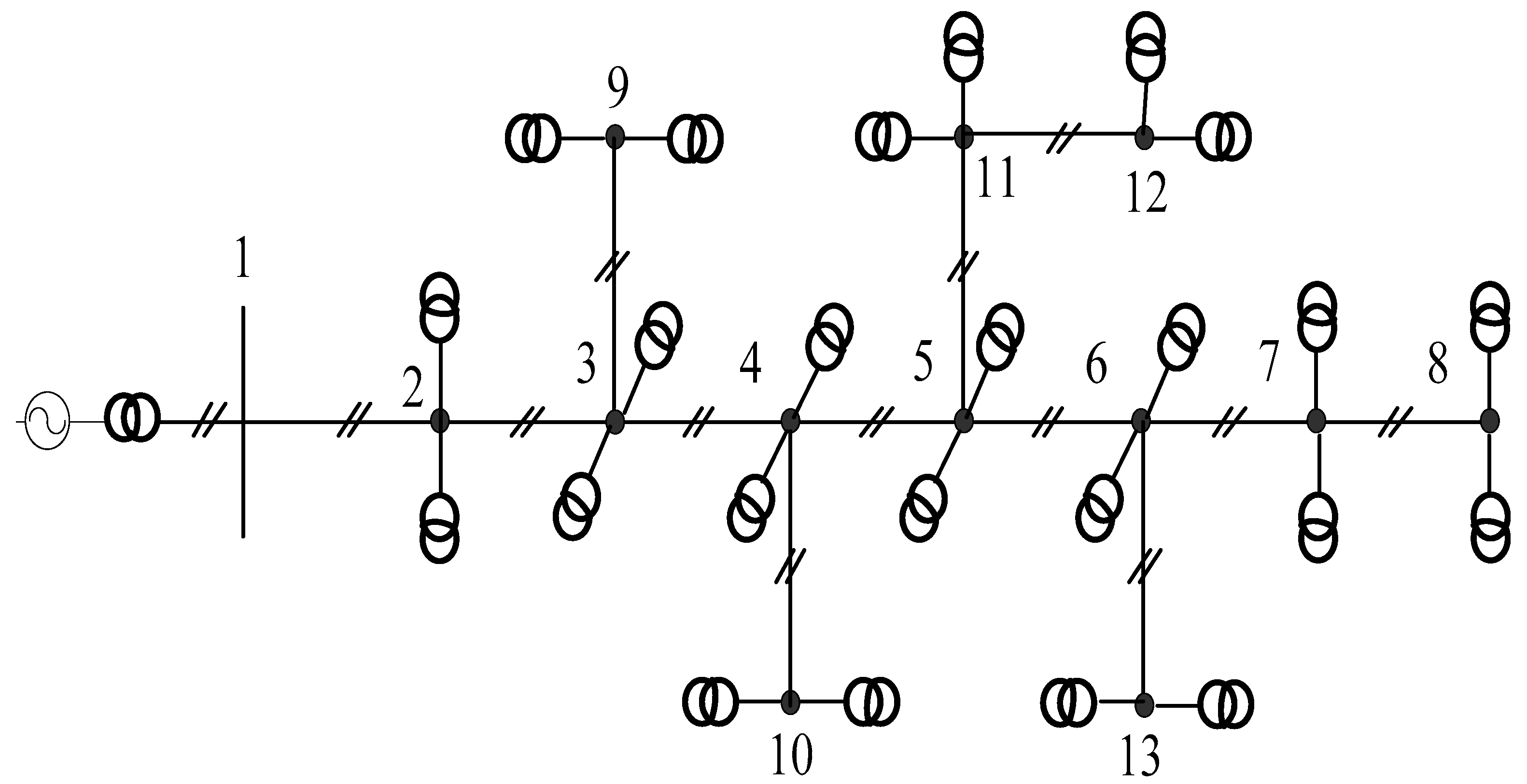
To evaluate the performance of the proposed method, many investigations were done based on different fault situations that can happen on a changed 13 bus IEEE network. This network was simulated in MATLAB and a π-line model was used in different sections. The tested system was a 13-bus system, and the distributed loads are shown in Figure 4. The length of each section is shown in Table 2. Each section of the lines was a π-model circuit. The number of the circuit presents the section of the line which it models. For each fault simulation, the voltage and current were measured and recorded from the local terminal. For this algorithm, the amplitude and phase of the three-phase’s voltage and current at the beginning of the feeder is required. These parameters were obtained from Fourier’s transform. To find the accuracy of the proposed method, the location’s error percentage is obtained by using the equation below:
4.2. Numerical Results
The effects of the fault’s distance, resistance, and angle at the beginning of the line on the proposed algorithm are studied in this section.
4.2.1. The Effect of the Fault’s Resistance
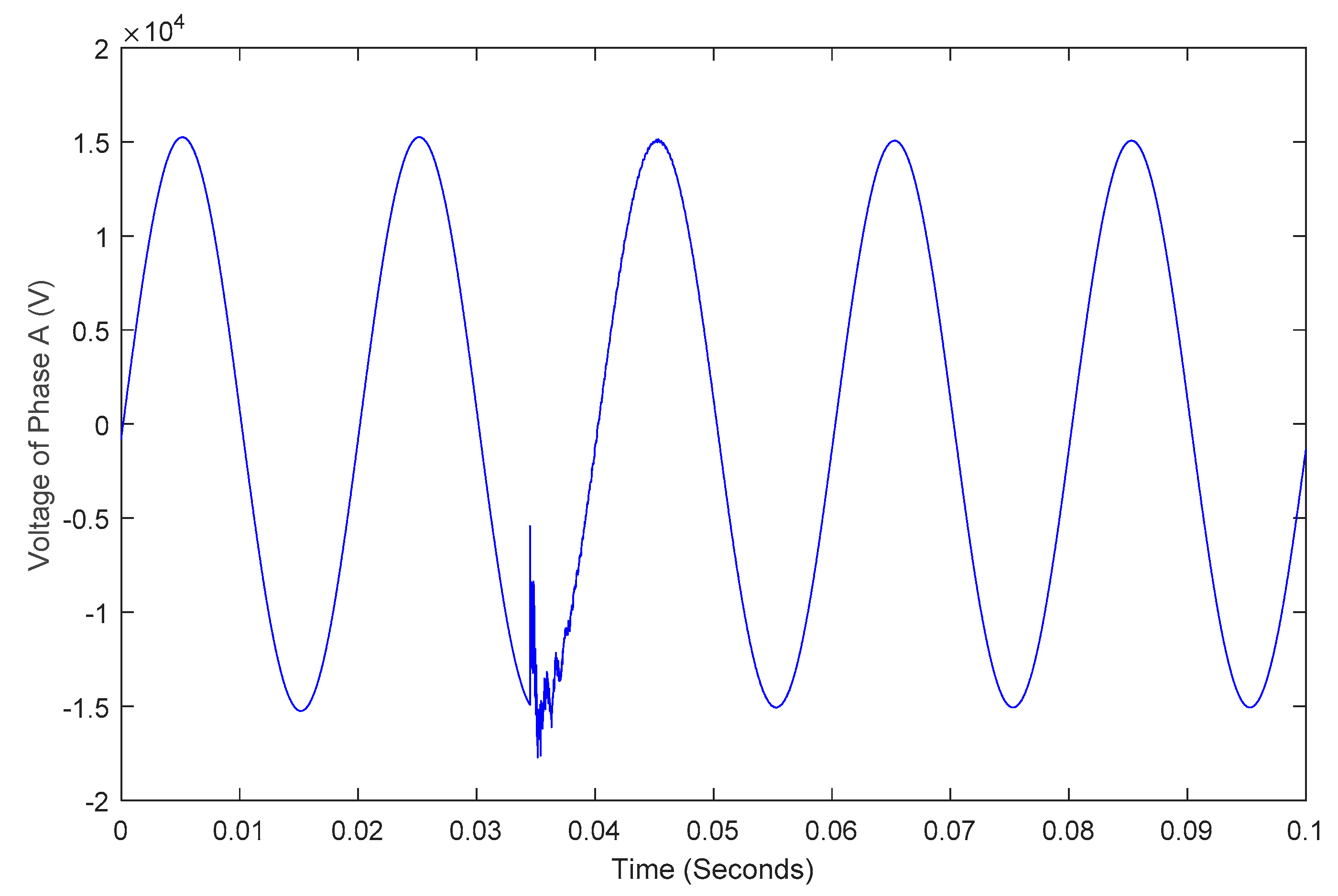
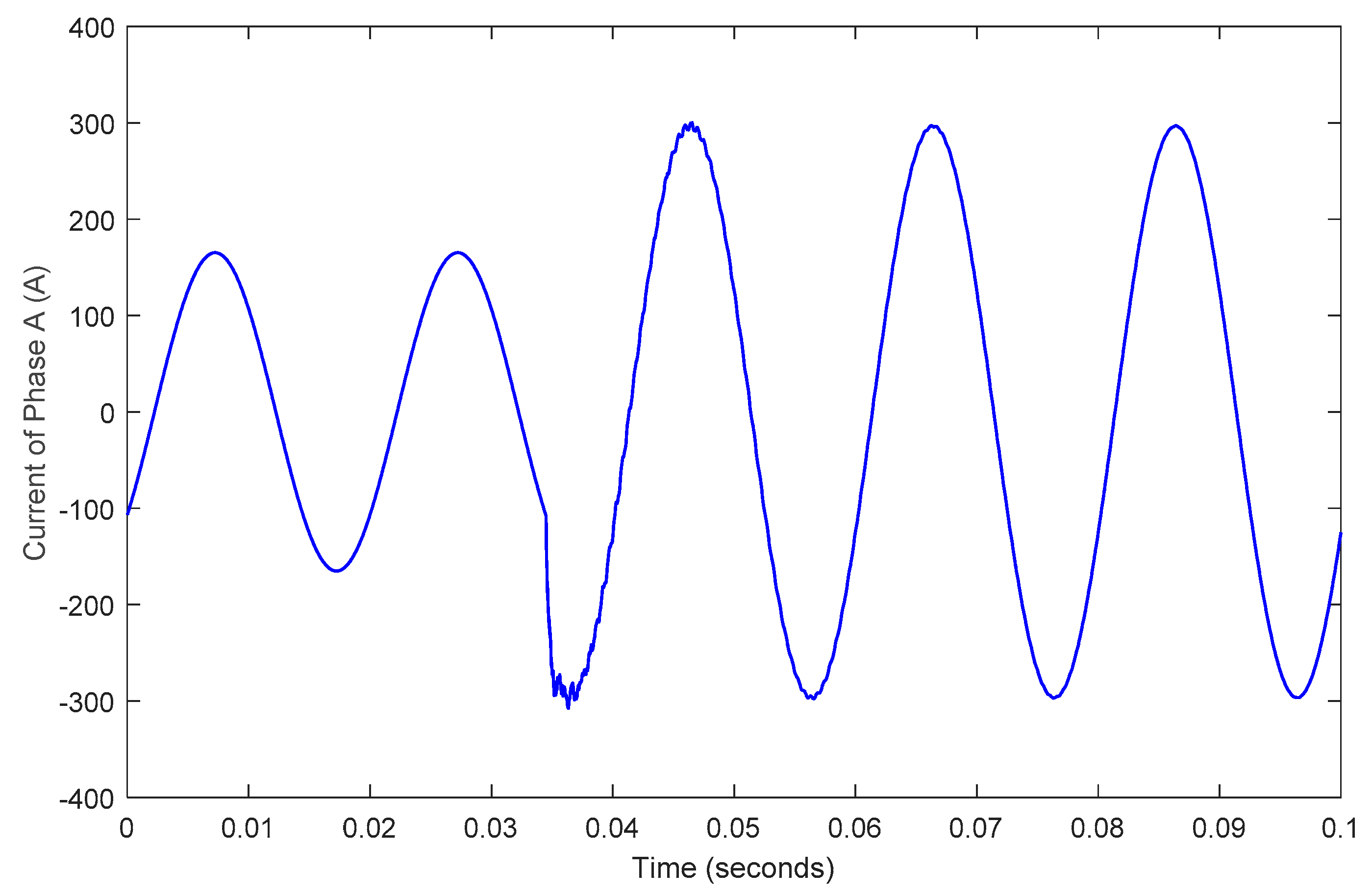
The fault’s resistance is one of the factors affecting the fault location’s accuracy. To evaluate the effect of the fault’s resistance, a simulation with single-phase faults to the ground with a range of resistances between 0 to 100 Ω was done. The results are shown in Figure 4. According to the results presented in Table 3, we can conclude that the fault’s resistance had little effect on the proposed method (even for larger than the average error percentage was very small, and the maximum error was also small), which shows the high precision of this method. Figure 5 and Figure 6 show the voltage and current at the beginning of the feeder for a single-phase short circuit fault to ground with 10 ohm fault resistance and 45 degree fault inception angle.
4.2.2. The Effect of the Fault’s Location
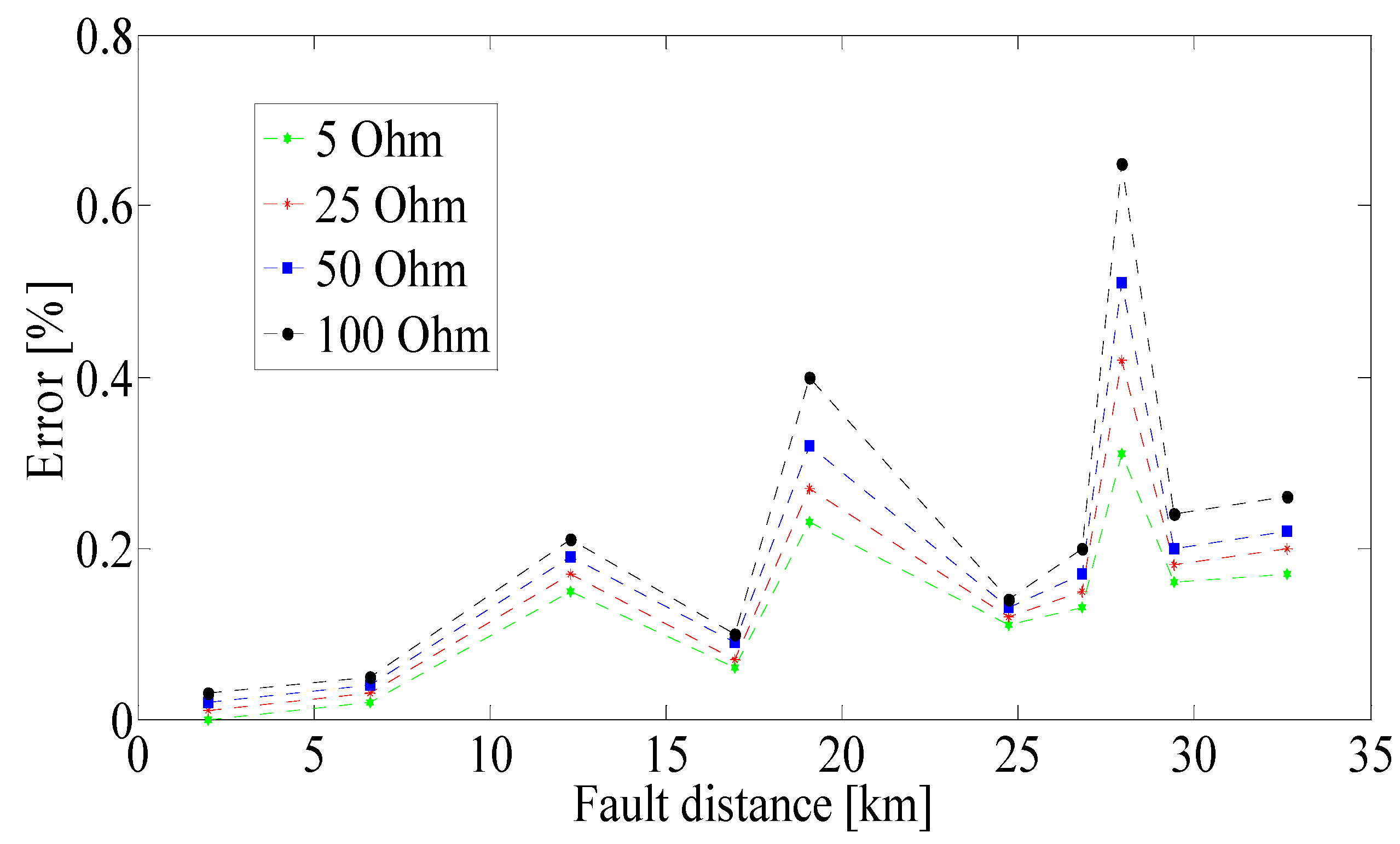
To determine how the suggested technique is sensitive to the fault occurrence locations, a simulation of single-phase faults to the ground on different sections of the medium power network was done. The results are presented in Figure 7. Single-phase to the ground fault simulations with an inception angle of 45 degrees, different resistances, and with various distances (5 km steps) from the beginning of the feeder to the end were done on the medium power network. Based on the presented results in Figure 7, we can conclude that the fault distance did not have a significant effect on the fault location method, and the maximum errors were from the subsidiary lines.
4.2.3. The Effect of the Fault’s Inception Angle
To determine how sensitive the proposed method is to the fault’s inception angle, various simulations were done. Table 4 shows the obtained results at fault inception angles of 0, 30, 45, and 90 degrees for single-phase to the ground faults with a resistance of 50 Ω. The simulation results show that the proposed method was not sensitive to the fault’s inception angle.
4.2.4. The Effect of Instruments Error
The accuracy of fault location algorithms depends on different parameters, such as the performance of measurement transformers (CTs, PTs). In this part, according to [13] the instrument transformers were modelled and simulated in MATLAB software according to CT error protection code is 5P20 and PT error class is 0.1%, It is done. The accuracy of the proposed method in different fault locations was analyzed, and the results are shown in Table 5. The obtained results show that the accuracy of the proposed method was high.
5. Conclusions
Double circuit lines are gaining popularity in distribution networks, mainly due to the increasing loads and the lack of public corridors. Automatic fault location in distribution networks is challenging, and it is even more difficult in double circuits than in single circuit lines. In this paper, a new fault location algorithm for double-circuit distribution networks is presented. In the proposed algorithm, a new quadratic equation is obtained using the power system equations and KVL and KCL. In this method, the voltage and current from the beginning of the feeder are used and the new equation is proved for calculating the equivalent impedance of each section. It is calculated using two over change the Fortescue transform to abs and upside. In the presented technique, the π line model, the lines’ capacitors effect, and the mutual effect of the lines on each other are considered. To the best of our knowledge, the improved algorithm is the first of its kind which supports double-circuit distribution networks. In this method, for each section of the distribution feeder, the proposed iterative algorithm is run and the location of the fault is determined. The maximum errors recorded from the faults were in T-offs, especially at the end of the T-offs. In our study, different fault distances, different resistances, and different inception angles were considered. The simulation results show that the maximum recorded error was 0.65%, which confirms a satisfactory performance.
For the future, our focus will be on the effect of DG on fault location in double circuit power distribution networks. We will also try to obtain a new and more accurate equation for locating faults in double circuit power distribution networks.
Author Contributions
Conceptualization, R.D. and S.M.S.; Methodology, R.D. and S.M.S.; Software, R.D. and S.M.S.; Formal Analysis, R.D., S.M.S., H.R.S. and M.T.; Investigation, S.M.S.; Resources, R.D., H.R.S. and M.T.; Writing-Original Draft Preparation, R.D. and S.M.S.; Writing-Review & Editing, M.T. and H.R.S.; Visualization, R.D. and S.M.S.; Supervision, R.D., H.R.S. and M.T.; Project Administration, R.D.; Funding Acquisition, R.D., H.R.S. and M.T.
Funding
This research received no external funding.
Conflicts of Interest
The authors declare no conflict of interest.
Nomenclature
| VSabc | voltage at the beginning of section |
| ISabc | current at the beginning of section |
| zzabc | matrix of line impedance |
| Yabc | admittance matrix or line capacitance |
| VRabc | voltage at the end of line |
| IRabc | current at the end of line |
| VS1,2,0 | positive, negative Seq. voltage at the beginning of section |
| IS1,2,0 | positive, negative Seq. injection current at the beginning of section |
| VF1,2,0 | positive, negative Seq. Fault point voltage at the fault point |
| IF1,2,0 | positive, negative Seq. injection current at the fault point |
| I | identity matrix |
| r | real parts |
| i | imaginary parts |
| lt | total length of feeder |
| Im | imaginary parts |
| Re | real parts |
| PDN | power distribution network |
| KCL | Kirchhoff’s current law |
| IL | load current |
| Iu | output current |
| IF | fault current |
| IBFLM | impedance-based fault location method |
| xactual | actual fault distance |
| Z1,0 | (positive, zero sequence of series impedance and parallel admittance of line) |
| Zm0 | (mutual sequence of impedance series of line) |
| Y1,0 | (Positive, zero sequence of parallel admittance of line) |
| Ym0 | (mutual sequence of parallel admittance of line) |
| xcalculated | calculated fault distance |
References
- Srinivasan, K.; Jacques, A. A new fault location algorithm for radial transmission lines with loads. IEEE Trans. Power Deliv. 1989, 4, 1676–1682. [Google Scholar]
- Das, R.; Sachdev, M.S.; Sidhu, T.S. A fault locator for radial subtransmission and distribution lines. In Proceedings of the Power Engineering Society Summer Meeting, Seattle, WA, USA, 16–20 July 2000; pp. 443–448. [Google Scholar]
- Yang, X.; Choi, M.S.; Lee, S.J.; Ten, C.W.; Lim, S.I. Fault location for underground power cable using distributed parameter approach. IEEE Trans. Power Syst. 2008, 23, 1809–1816. [Google Scholar] [CrossRef]
- Filomena, A.D.; Resener, M.; Salim, R.H.; Bretas, A.S. Fault location for underground distribution feeders: An extended impedance-based formulation with capacitive current compensation. Int. J. Electr. Power Energy Syst. 2009, 31, 489–496. [Google Scholar] [CrossRef]
- Lee, S.J.; Choi, M.S.; Kang, S.H.; Jin, B.G.; Lee, D.S.; Ahn, B.S.; Yoon, N.S.; Kim, H.S.; Wee, S.B. An intelligent and efficient fault location and diagnosis scheme for radial distribution systems. IEEE Trans. Power Deliv. 2004, 19, 524–532. [Google Scholar] [CrossRef]
- Salim, R.H.; Wang, B.; Liu, D.; Gou, S. Further improvements on impedance-based fault location for power distribution systems. IET Gen. Transm. Distrib. 2011, 5, 467–478. [Google Scholar] [CrossRef]
- Dashti, R.; Sadeh, J. Accuracy improvement of impedance based fault location method for power distribution network using distributed-parameter line model. Int. Trans. Electr. Energy Syst. 2012, 24, 318–334. [Google Scholar] [CrossRef]
- Dashti, R.; Sadeh, J. Applying dynamic load estimation and distributed parameter line model to enhance the accuracy of impedance based fault location methods for power distribution networks. Electr. Power Compon. Syst. 2013, 41, 1334–1362. [Google Scholar] [CrossRef]
- Dashti, R.; Sadeh, J. Fault section estimation in power distribution network using impedance-based fault distance calculation and frequency spectrum analysis. IET Gen. Transm. Distrib. 2014, 8, 1406–1417. [Google Scholar] [CrossRef]
- Orozco-Henao, C.; Bretas, A.S.; Chouhy-Leborgne, R.; Herrera-Orozco, A.R.; Marín-Quintero, J. Active distribution network fault location methodology: A minimum fault reactance and Fibonacci search approach. Int. J. Electr. Power Energy Syst. 2017, 84, 232–241. [Google Scholar] [CrossRef]
- Liang, R.; Wang, F.; Fu, G.; Xue, X.; Zhou, R. A general fault location method in complex power grid based on wide-area traveling wave data acquisition. Int. J. Electr. Power Energy Syst. 2016, 83, 213–218. [Google Scholar] [CrossRef]
- Jamali, S.; Bahmanyar, A. A new fault location method for distribution networks using sparse measurements. Int. J. Electr. Power Energy Syst. 2016, 81, 459–468. [Google Scholar] [CrossRef]
- Sarwat, A.I.; Amini, M.; Domijan, A.; Damnjanovic, A.; Kaleem, F. Weather-based interruption prediction in the smart grid utilizing chronological data. J. Mod. Power Syst. Clean Energy 2015, 4, 308–315. [Google Scholar] [CrossRef] [Green Version]
- Kezunovic, M.; Abur, A.; Kojovic, L.J.; Skendzic, V.; Singh, H. DYNA-TEST simulator for relay testing, part II: Performance evaluation. IEEE Trans. Power Deliv. 1992, 7, 1097–1103. [Google Scholar] [CrossRef]
- Daisy, M.; Dashti, R. Single phase fault location in electrical distribution feeder using hybrid method. Energy 2016, 103, 356–368. [Google Scholar] [CrossRef]
- Dashti, R.; Daisy, M.; Shaker, H.R.; Tahavori, M. Impedance-Based Fault Location Method for Four-Wire Power Distribution Networks. IEEE Access 2018, 6, 1342–1349. [Google Scholar] [CrossRef]
- Cifuentes-Chaves, H.; Mora-Flórez, J.; Pérez-Londoño, S. Time domain analysis for fault location in power distribution systems considering the load dynamics. Electr. Power Syst. Res. 2017, 146, 331–340. [Google Scholar] [CrossRef]
- Bahmanyar, A.; Jamali, S. Fault location in active distribution networks using non-synchronized measurements. Electr. Power Energy Syst. 2017, 93, 451–458. [Google Scholar] [CrossRef]
- Dashti, R.; Ghasemi, M.; Daisy, M. Fault Location in Power Distribution Network with Presence of Distributed Generation Resources Using Impedance Based Method and Applying π Line Model. Energy 2018, in press. [Google Scholar] [CrossRef]
- De Aguiar, R.A.; Dalcastagnê, A.L.; Zürn, H.H.; Seara, R. Impedance-based fault location methods: Sensitivity analysis and performance improvement. Electr. Power Syst. Res. 2018, 155, 236–245. [Google Scholar] [CrossRef]
- Gabr, M.A.; Ibrahim, D.K.; Ahmed, E.S.; Gilany, M.I. A new impedance-based fault location scheme for overhead unbalanced radial distribution networks. Electr. Power Syst. Res. 2017, 142, 153–162. [Google Scholar] [CrossRef]
- Chen, R.; Lin, T.; Bi, R.; Xu, X. Novel Strategy for Accurate Locating of Voltage Sag Sources in Smart Distribution Networks with Inverter-Interfaced Distributed Generators. Energies 2017, 10, 1885. [Google Scholar] [CrossRef]
- Deng, X.; Yuana, R.; Xiaob, Z.; Li, T.; Wang, K.L.L. Fault location in loop distribution network using SVM technology. Electr. Power Energy Syst. 2015, 65, 254–261. [Google Scholar] [CrossRef]
- Liang, R.; Fu, G.; Zhu, X.; Xue, X. Fault location based on single terminal travelling wave analysis in radial distribution network. Electr. Power Energy Syst. 2015, 66, 160–165. [Google Scholar] [CrossRef]
- Alamuti, M.M.; Nouri, H.; Ciric, R.M.; Terzija, V. Intermittent fault location in distribution feeders. IEEE Trans. Power Deliv. 2012, 27, 96–103. [Google Scholar] [CrossRef]
Figure 1.
(a) Single-line diagram for each section of a power distribution system; (b) Positive; (c) negative; and (d) zero-sequence networks of a double-circuit distribution line during a usual fault.
Figure 1.
(a) Single-line diagram for each section of a power distribution system; (b) Positive; (c) negative; and (d) zero-sequence networks of a double-circuit distribution line during a usual fault.

Figure 2.
General view of ground faults (single phase, two phase, and three-phase fault to the ground).
Figure 2.
General view of ground faults (single phase, two phase, and three-phase fault to the ground).

Figure 3.
Flowchart of the proposed method.

Figure 4.
The studied distribution feeder (the numbers is nodes number).

Figure 5.
The recorded faulty phase voltage at the beginning of the feeder (in 21.06 km).

Figure 6.
The recorded faulty phase current at the beginning of the feeder (in 21.06 km).

Figure 7.
Error percentage of the proposed method for various resistances and different locations.


Table 1.
Comparison of different power distribution fault-location methods.
| Proposed Method | Dashti et al., 2018 [19] | Aguiar et al. (2018) [20] | Dashti et al. (2018) [16] | Gabr et al., 2017 [21] | Chen et al. (2017) [22] | Daisy et al., 2016 [15] | Deng et al., 2015 [23] | Rui et al., 2015 [24] | Dashti et al., 2012 [7] | Dashti et al., 2013 [8] | Alamiti et al., 2012 [25] | Salim et al. (2011) [6] | Reference |
|---|---|---|---|---|---|---|---|---|---|---|---|---|---|
| π model | π model | DPLM a | DPLM a | short line model | short line model | DPLM a | DPLM a | π model | DPLM a | DPLM a | DPLM | π model | Line model |
| constant load | constant load | constant load | static load | constant load | constant load | static load | constant load | constant load | constant load | static load | static load | static load | Load model |
| - | - | - | - | - | - | √ | - | - | - | √ | √ | √ | Load estimation |
| √ | √ | - | √ | √ | - | √ | - | - | √ | √ | - | √ | Non-homogeneity |
| √ | √ | - | √ | - | - | √ | - | - | √ | √ | - | √ | Unbalanced system |
| √ | √ | √ | √ | √ | √ | √ | - | √ | √ | √ | - | √ | Laterals |
| √ | √ | - | √ | √ | √ | √ | √ | - | √ | √ | - | √ | Load taps |
| All | All | All | All | All | All | SLG d | SLG d | All | All | All | All | All | Fault type |
| - | - | - | - | - | - | Voltage sag | Support vector machine | - | - | CP b and PD c | - | - | Section detection |
| Radial | Radial and loop | Radial | Radial | Radial | Radial | Radial | loop | Radial | Redial | Redial | Redial | Redial | Network Type |
| - | √ | - | - | - | √ | - | √ | - | - | - | - | - | Smart Grid |
| - | √ | - | - | - | √ | - | - | - | - | - | - | Distributed generation | |
| - | - | - | - | - | - | - | - | √ | - | - | √ | - | Time domain |
| √ | √ | √ | √ | √ | √ | √ | √ | - | √ | √ | - | √ | Phase domain |
| - | - | - | - | - | - | √ | √ | - | - | - | - | - | Sequence domain |
a DPLM = distributed–parameter line model; b CP = current pattern; c PD = protective devices; d SLG = single-phase-to ground fault.
Table 2.
Length of the lines.
| Bus from | Bus to | Distance (km) | Bus from | Bus to | Distance (km) |
|---|---|---|---|---|---|
| 1 | 2 | 4.6 | 5 | 6 | 3.2 |
| 2 | 3 | 4.6 | 5 | 11 | 2.6 |
| 3 | 4 | 7.763 | 6 | 7 | 2.6 |
| 3 | 9 | 5.1 | 6 | 13 | 3 |
| 4 | 5 | 7.763 | 7 | 8 | 4 |
| 4 | 10 | 5 | 11 | 12 | 2 |
Table 3.
The error percentage of different faults at various resistances.
| Fault Resistance (Ω) | Fault Distance (km) | Fault Type | |||
|---|---|---|---|---|---|
| Single-Phase to the Ground | Two Phases to the Ground | Two Phases to Each Other | Three Phases to the Ground | ||
| Error Percentage | |||||
| 0 | 6.6 | 0.00 | 0.00 | 0.00 | 0.00 |
| 16.96 | 0.02 | 0.02 | 0.02 | 0.03 | |
| 26.82 | 0.09 | 0.08 | 0.10 | 0.11 | |
| 32.62 | 0.07 | 0.06 | 0.06 | 0.08 | |
| 25 | 6.6 | 0.03 | 0.02 | 0.01 | 0.01 |
| 16.96 | 0.05 | 0.04 | 0.02 | 0.03 | |
| 26.82 | 0.14 | 0.20 | 0.20 | 0.35 | |
| 32.62 | 0.11 | 0.17 | 0.22 | 0.22 | |
| 50 | 6.6 | 0.03 | 0.02 | 0.01 | 0.01 |
| 16.96 | 0.05 | 0.04 | 0.02 | 0.03 | |
| 26.82 | 0.14 | 0.20 | 0.20 | 0.35 | |
| 32.62 | 0.11 | 0.17 | 0.22 | 0.22 | |
| 100 | 6.6 | 0.05 | 0.04 | 0.04 | 0.05 |
| 16.96 | 0.09 | 0.08 | 0.08 | 0.08 | |
| 26.82 | 0.44 | 0.64 | 0.62 | 0.96 | |
| 32.62 | 0.29 | 0.22 | 0.23 | 0.23 | |
Table 4.
Effect of fault inception angle on the proposed method.
| Average Error Percentage (%) | Maximum Error Percentage (%) | Fault Inception Angle Degrees |
|---|---|---|
| 0/19 | 0/51 | 0 |
| 0/18 | 0/50 | 30 |
| 0/19 | 0/49 | 45 |
| 0/17 | 0/50 | 90 |
Table 5.
Results of running the proposed algorithm considering measurement error.
| Fault Location (km) | Fault Type | |||
|---|---|---|---|---|
| Single-Phase to Ground | Double-Phase to Each Other | Double-Phase to Ground | Three Phases to Ground | |
| Average Error Percentage | ||||
| 6 | 0.0821 | 0.1380 | 0.1105 | 0.0683 |
| 12 | 0.1202 | 0.2103 | 0.2055 | 0.1352 |
| 22 | 0.9577 | 0.7376 | 0.7352 | 0.5015 |
| 30 | 1.0751 | 0.9100 | 0.9098 | 0.6872 |
© 2018 by the authors. Licensee MDPI, Basel, Switzerland. This article is an open access article distributed under the terms and conditions of the Creative Commons Attribution (CC BY) license (http://creativecommons.org/licenses/by/4.0/).
Share and Cite
MDPI and ACS Style
Dashti, R.; Salehizadeh, S.M.; Shaker, H.R.; Tahavori, M. Fault Location in Double Circuit Medium Power Distribution Networks Using an Impedance-Based Method. Appl. Sci. 2018, 8, 1034. https://doi.org/10.3390/app8071034
AMA Style
Dashti R, Salehizadeh SM, Shaker HR, Tahavori M. Fault Location in Double Circuit Medium Power Distribution Networks Using an Impedance-Based Method. Applied Sciences. 2018; 8(7):1034. https://doi.org/10.3390/app8071034
Chicago/Turabian StyleDashti, Rahman, Seyed Mehdi Salehizadeh, Hamid Reza Shaker, and Maryamsadat Tahavori. 2018. "Fault Location in Double Circuit Medium Power Distribution Networks Using an Impedance-Based Method" Applied Sciences 8, no. 7: 1034. https://doi.org/10.3390/app8071034
Note that from the first issue of 2016, this journal uses article numbers instead of page numbers. See further details here.