GNSS-Based Verticality Monitoring of Super-Tall Buildings


1
Department of Surveying Engineering, Guangdong University of Technology, No. 100 Waihuan Xi Rd., Panyu District, Guangzhou 510006, China
2
Guangzhou Urban Planning & Design Survey Research Institute, No. 10 Jianshedama Rd., Guangzhou 510006, China
3
College of Surveying and Geo-Informatics, Tongji University, No. 1239 Siping Rd., Yangpu District, Shanghai 200092, China
*
Author to whom correspondence should be addressed.
Appl. Sci. 2018, 8(6), 991; https://doi.org/10.3390/app8060991
Submission received: 30 March 2018
/
Revised: 30 May 2018
/
Accepted: 14 June 2018
/
Published: 16 June 2018
(This article belongs to the Special Issue Structural Damage Detection and Health Monitoring)
Abstract
:In the construction of super-tall buildings, it is rather important to control the verticality. In general, a laser plummet is used to transmit coordinates of reference points from the ground layer-by-layer, which can effectively control the verticality of super-tall buildings. However, the errors in transmission will accumulate with increasing height and motion of the buildings in construction. This paper presents a global navigation satellite system (GNSS)-based method to check the results of laser plumbing. The method consists of four steps: (1) Computing the coordinate time series of monitoring points by adjusting the GNSS monitoring network observations at each epoch; (2) Analyzing the horizontal motion of super-tall buildings and its effect on vertical reference transmission; (3) Calculating the deflections of the vertical at the monitoring point using an Earth gravity field model and a geoid model. With deflections of the vertical, the static GNSS-measured coordinates are aligned to the same datum as used by the laser plummet; and (4) Finally, validating/checking the result of laser plumbing by comparing it with static GNSS results corrected by deflections of the vertical. A case study of a 438-m high building is tested in Guangzhou, China. The result demonstrates that the gross errors of baseline vectors can be eliminated effectively by GNSS network adjustment of the first step. The two-dimensional displacements can be measured at millimeter-level accuracy; the difference between the coordinates of the static GNSS measurement and laser plumbing is less than ±2.0 cm after correction with the deflections of the vertical, which meets the design requirement of ±3.0 cm according to the Technical Specification for Concrete Structures of Tall Buildings in China.
1. Introduction
A Global Navigation Satellite System (GNSS) is a positioning technology widely used for monitoring displacement of large civil engineering structures, such as dams [1,2,3,4] and bridges [5,6,7,8,9]. In recent decades, a larger number of super-tall buildings have been built in modern cities worldwide; for instance, the 828-m high Burj Khalifa (Dubai) and the 438-m high Guangzhou International Finance Center (China). To maintain the safe construction and running of these super-tall buildings, monitoring deformation under varying environmental conditions is a very important issue. Lovse et al. [10], Tamura et al. [11], Casciati and Fuggini [12], and Yi et al. [13] applied GNSS to measure the displacement responses of super-tall buildings under the effects of wind, construction load, temperature, and sun exposure. In addition, Tang et al. [14] have investigated real-time kinematic PPP (Precise Point Positioning) GPS for structure monitoring, and Sampietro et al. [15] studied the use of low-cost GNSS receivers to monitor surface deformations, which may be an important topic for future experiments. The comparison between GNSS and acceleration by Chan et al. [16] and Li et al. [17] reveals their high consistency, which also implies that GNSS can effectively monitor the motion of super-tall buildings. The real-time kinematic (RTK) positioning technique (e.g., network RTK GNSS) is widely used for obtaining the coordinates of monitoring points in real time [18,19]. RTK has several advantages, such as flexibility and the real-time acquisition of coordinates.
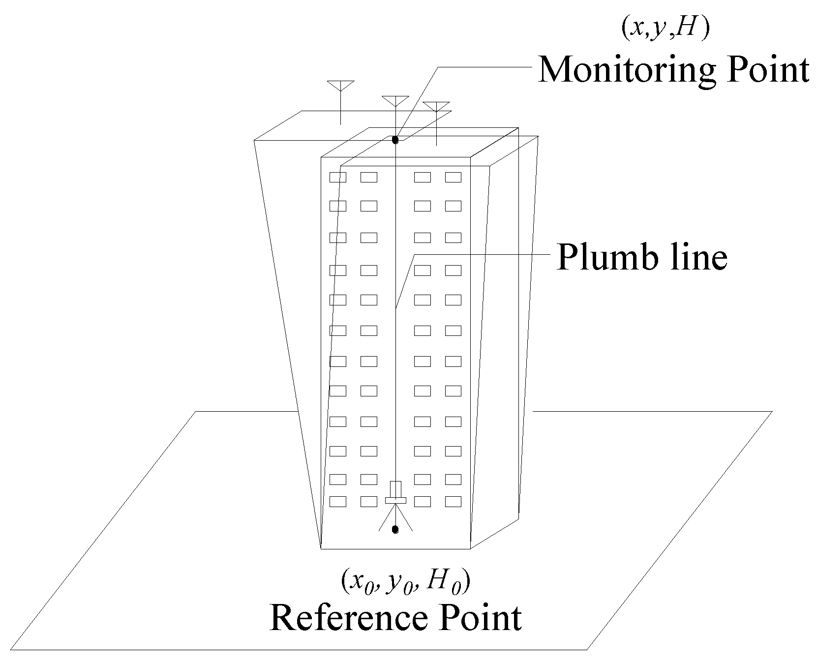
During a super-tall building’s construction, a laser plummet is usually used to transmit the coordinates of reference points from the ground layer-by-layer, which effectively controls the verticality of super-tall buildings. However, motion of super-tall buildings in a horizontal plane will occur due to such external factors as tower crane operation, wind, construction load, temperature, and sun exposure during construction as shown in Figure 1. In this case, it is difficult to accurately transmit the coordinates of reference points by laser plummet, and the plumbing accuracy would be severely affected by the transmitted errors as the height of the building increases. Therefore, monitoring the motion of super-tall buildings in a horizontal plane and checking the result of a laser plumbing point based on GNSS technology is extremely important.
In fact, the GNSS results refer in many cases to an ellipsoidal reference system while the laser plummet refers to a geoidal system. In order to check the result of a laser plumbing point based on GNSS technology, their results need to be matched into a unique datum with deflections of the vertical. For instance, the gravity vector has been considered during the construction of the 828-m high Burj Khalifa [20]. Therefore, the determination of the deflections of the vertical is very important work. Traditionally, the deflection of vertical components are determined from astro-geodesy [21,22,23], gravimetry [24,25], GNSS/leveling [26,27], etc. from which it is easier to calculate the deflections of the vertical with an Earth gravity field model and a geoid model.
As a case study, this paper aims to monitor the verticality of the 438-m high Guangzhou International Finance Center based on GNSS technology. The paper is organized as follows: first, the data processing strategy for calculating the monitoring point’s coordinate time series and deflections of the vertical are introduced, and we match the results of static GNSS Measurements and Laser Plumbing with deflection of the vertical components obtained from an Earth gravity field model (e.g., EGM2008) and a geoid model (e.g., GZGEOID). Finally, we analyze the horizontal motion of the Guangzhou International Finance Center and check its verticality based on static GNSS technology.
2. Calculation of the Monitoring Point’s Coordinate Time Series
In order to estimate the motion of a super-tall building, it is necessary to calculate the monitoring points’ coordinates time series. For this purpose, the coordinate time series of monitoring points are obtained by adjusting the GNSS monitoring network composed of three reference stations and one monitoring station at each epoch. According to the coordinate time series of the monitoring points, the authors can analyze the horizontal motion of a super-tall building and its effect on vertical reference transmission. The flowchart diagram of the GNSS processing strategy is shown in Figure 2. The GNSS data is post-processed in a kinematic mode to obtain the epoch wise baseline vectors and covariance matrix between the monitoring station and three reference stations. All these baselines form a GNSS monitoring network, including the baseline vectors and covariance matrix between the three reference stations solved in a static mode. Then, eliminating the gross errors of baseline vectors according to the misclosures and fixing the coordinates of the reference points obtained from the construction control network, the coordinate time series of each monitoring point are obtained by a constrained GNSS network adjustment. Finally, the precise coordinates of a monitoring point are obtained by the Daubechies wavelet filter, which allows us to analyse the horizontal motion of a super-tall building.
2.1. Criteria of Eliminating the Gross Errors
Before eliminating the gross error of baseline vectors, we construct a closed loop with the reference network and the baseline vectors between the monitoring and reference stations at each epoch. In this paper, three-dimensional baseline vectors and a covariance matrix will be directly used for GNSS network adjustment according to the Specifications for global positioning system (GPS) surveys in China, and we can assume that the closed loop consists of n baselines. Then, the misclosures are computed in three coordinate components as:
Assuming that the baseline vectors with a different precision are not correlated, the tolerance of misclosures reads as follows [28]:
where , , a is the constant error of GNSS receivers in millimeters (a = 5 mm for static mode and a = 10 mm for kinematic mode), b is the coefficient of ratio error in ppm (b = 1 ppm for static and kinematic mode), and d is the length of the baseline in kilometers.
According to the error-processing criterion, if the misclosure is 3 times larger than the STD of the misclosure, then all baselines in the closed loop can be considered unqualified. After rejecting the baselines by checking the formed closed loop, the remaining baselines are all qualified. Since the above process is based on the WGS-84 system, one can of course transform the baseline results as well as the closed loops into a Gaussian plane coordinate system (wx, wy, wH) as follows [28]:
where the transformation matrices RB and Rg are given by [28]
where Bk and Lk are the latitude and longitude of station k, respectively, l is the difference of longitude between station k and the central meridian used for projection, and M and N are the radii of curvature in the meridian and prime verticals, respectively.
A minimally constrained least-squares adjustment (free network adjustment) is performed. The residuals that result from this adjustment are strictly related to the baseline vectors. These residuals are examined, and from them blunders that may have gone undetected through the analyses of misclosures can be found and eliminated. The baseline vector correction tolerances are as follows:
where is the precision of the baseline vectors.
2.2. GNSS Monitoring Network Adjustment and Noise Filtering
First of all, GNSS data is processed in the post-processed kinematic mode to obtain the baseline vectors of the monitoring station to three reference stations epoch-by-epoch. Secondly, we identify and eliminate gross errors of baseline vectors by the misclosures and a minimally constrained least-squares adjustment epoch-by-epoch. Finally, we use the reference points’ coordinates obtained from the construction control network as constraints and then process the GNSS monitoring network data with a least-squares adjustment at each epoch based on the qualified baseline vectors and their variance information [28]. Nevertheless, the coordinate time series of monitoring points contains not only the real displacements of super-tall buildings, but also the measurement noise (e.g., GNSS phase noise). The displacement of the monitoring point is characterized by systematic signal even though it may be small over a short time period, but the measurement noise is characterized by strong noise that can be reduced by wavelet filtering. The choice of an appropriate wavelet basis function and the best decomposition level are the main issues in wavelet analysis. The compactly supported orthogonal Daubechies wavelet is widely applied in the field of engineering [29,30] since it gives accurate results in time-frequency analysis. Regarding the choice of decomposition level, we take into account both the signal change and the data-sampling rate.
3. Matching the Results of Static GNSS Measurements and Laser Plumbing
In fact, the GNSS results refer in many cases to an ellipsoidal reference system, while the laser plummet refers to a geoidal system. Therefore, their results need to be matched into a unique datum with deflections of the vertical, i.e., the plumb line.
3.1. Determination of Deflection of the Vertical Components
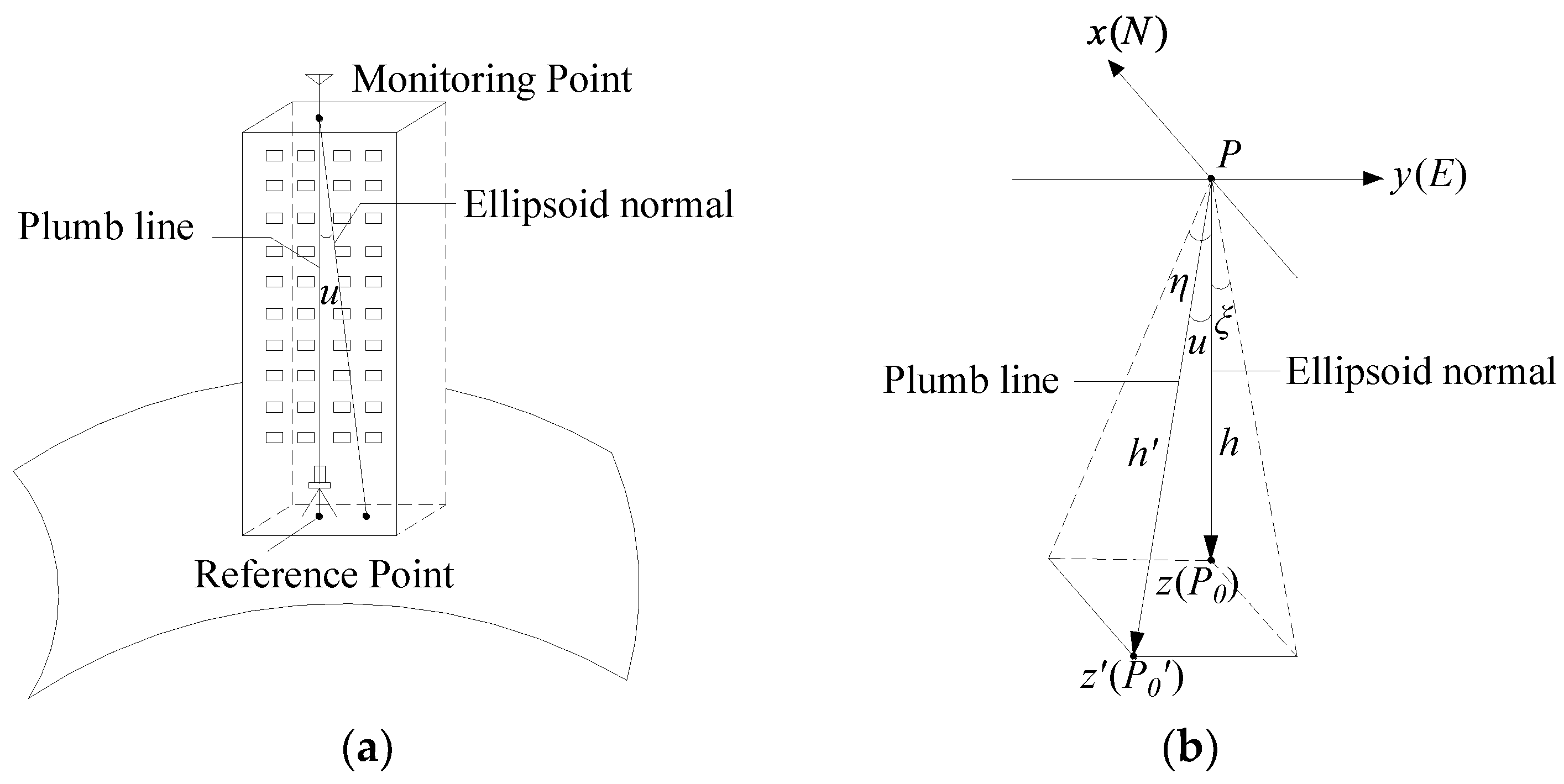
As shown in Figure 3, the deflection of the vertical u is the angle between the gravity vector at a reference point and the ellipsoidal normal through the same point for a particular ellipsoid. It is conventionally decomposed into two perpendicular components: a north-south meridional component ξ and an east-west prime vertical component η. In this paper, the deflections of vertical are determined from an Earth gravity field model and a geoid model.
By using a set of Earth gravity field coefficients (e.g., EGM2008), one can calculate the deflection of the vertical component ξ along the meridian and η along the prime vertical as: [25]
where Nmax is the maximum degree of the Earth gravity field model, n = µ = max (2, m), GM is the geocentric gravitational constant; a is the specific scale parameter of the Earth global gravitational model. ϕ, λ, and r are the latitude, longitude, and geocentric radius of the spherical coordinates for the computation point, respectively, is the normal gravity at (ϕ,λ, r), are the fully normalized associated Legendre functions of degree n and order m, and and are the fully normalized spherical harmonic coefficients referred to some normal gravity field.
Assume that we have two closely spaced locations A and B on the surface of the earth with their geoid height difference and geodetic azimuth . One computes the deflection of the vertical component along the meridian and along the prime vertical as [26]
where is the deflection of the vertical and is the length of the corresponding geodesic arc. can be obtained from the precise leveling and GNSS measurements . As an alternative, the geoid height difference can be calculated by a geoid model.
When we apply an error distribution to Equation (10), and omit the effect of distance , the error formula can be written as follows:
For instance, for and , the standard deviation of the calculated deflection of the vertical would be about arc seconds.
3.2. Bias Correction of GNSS Measurements and Laser Plumbing
To make use of GNSS surveying to check the plumbing result of a laser plummet, we need to eliminate the systematic bias of GNSS affected by deflections of the vertical. In other words, the GNSS coordinates should be transformed into a system with the same datum.
As shown in Figure 3b, the deflection of the vertical u is decomposed into two perpendicular components: a north-south meridional component ξ (the positive direction is toward the south) and an east-west prime vertical component η (the positive direction is toward the west). The geodetic coordinates P-xyz are related to the normal ellipsoid. The z-axis points toward the interior of the ellipsoid along the ellipsoid normal. The z′-axis points toward the interior of the geoid along the plumb line. The x-axis points toward the north (N) and the y-axis points east (E) to form an orthogonal, right-handed rectangular coordinate system. The points P0 and P0′ are the projections from the point P along the z-axis and the z′-axis, respectively. The projection heights of the points P0 and P0′ are expressed by h and h′, respectively. In general, the deflection of the vertical is so small (e.g., 10 arc seconds) that the projection heights h and h′ (with a building height of 432 m, the difference between h and h′ is about 2 cm) are approximately equal; therefore, the effect of curvature of the plumb line is neglected in this paper.
The plane-coordinate difference between the points P0 and P0′ can be approximately calculated as
Therefore, the authors can assess the systematic bias between the coordinates of the GNSS measurement and laser plumbing using Equations (12) and (13).
In order to analyze the systematic bias between the coordinates of the GNSS measurement and laser plumbing at different building heights, the authors can assume that a building (23°02′24.17311” N, 113°23′43.95410” E) located at Guangzhou city has different heights. Then, the deflection of the vertical components can be calculated by Equations (8) and (9) with the Earth Gravitational Model EGM2008 (to degree 2160) [31] at different heights (e.g., H = building height). Finally, an approximation of the systematic bias between the coordinates of the GNSS measurement and laser plumbing can be calculated by Equations (12) and (13). Table 1 lists the approximations of the systematic bias in the x and y directions at different building heights.
Referring to the values listed in Table 1, one may see that the systematic bias between the coordinates of the GNSS measurement and laser plumbing is small when the building height is smaller than 100 m for a building in Guangzhou. However, the systematic bias increases with an increase in building height when the building height exceeds 100 m. Therefore, the systematic bias cannot be ignored in verticality monitoring of super-tall buildings.
4. Simulation
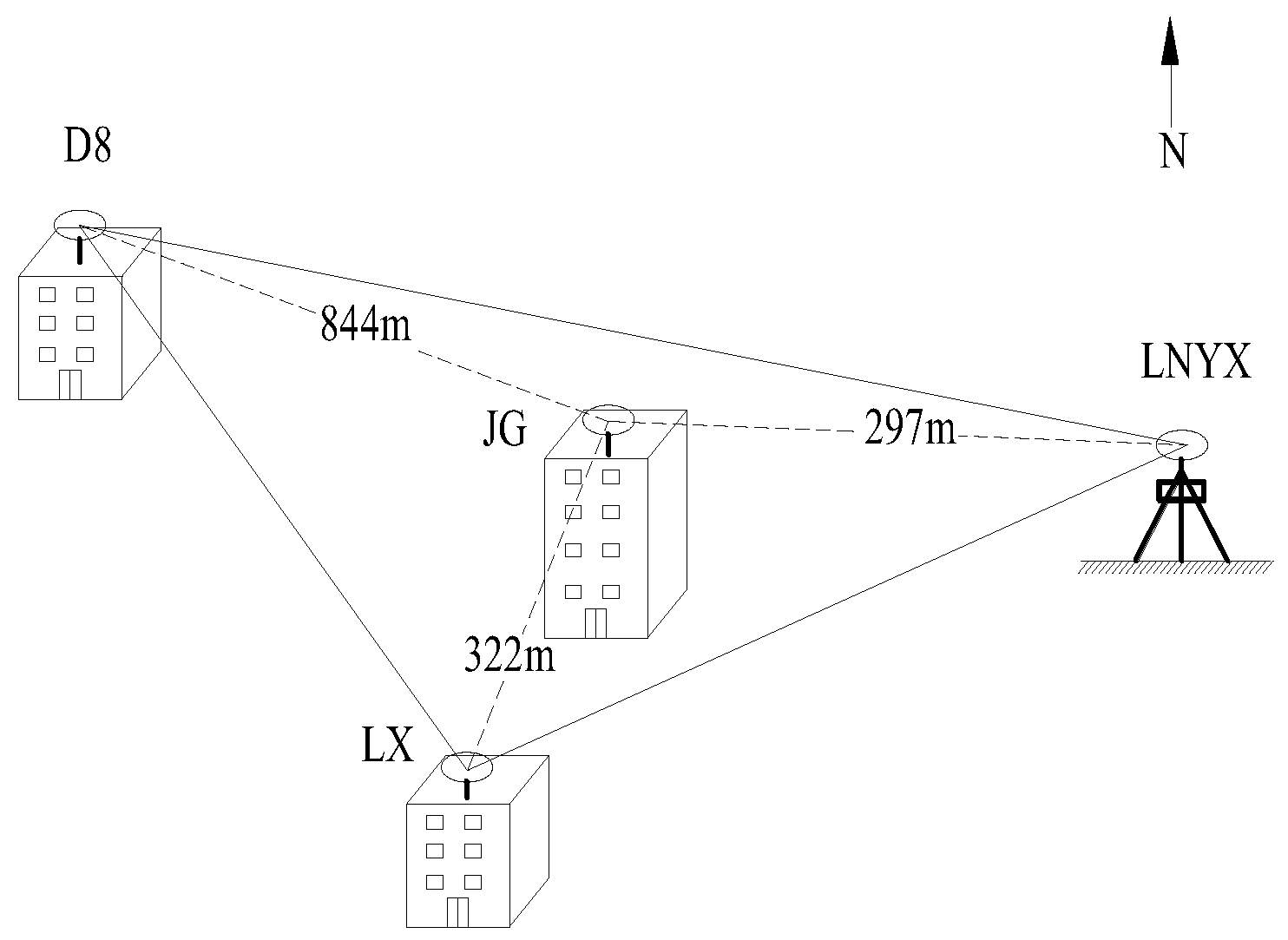
Before applying the method in this paper to super-tall buildings, a simulation is first conducted to show the efficiency of the method. The goal of this simulation is to analyze the displacements of the stable JG building with a height of 10 m located at the Guangdong University of Technology. This building is held up by a reinforced concrete structure. On its roof, a GNSS station was installed to monitor the building’s displacements. In addition, we established a reference network around the JG building consisting of three reference points, D8, LNYX, and LX. We chose these locations based on their suitability as reference stations according to the International GNSS service (IGS) criteria, keeping in mind the difficulty of finding adequate locations in an urban setting. Figure 4 shows the locations of the three points of the reference network and their distances to the JG building. Two points, D8 and LX, were located on low concrete buildings and one, LNYX, on a metal stand at ground level. Dual-frequency Trimble R8 GNSS receivers were employed to collect data for 2 h with a sampling interval of 1 s at all stations. As per the prior information, it is reasonable to assume that the displacement of the JG building is small or even negligible due to its low height and nonexposure to the effects of construction load, sun exposure, etc.
The GNSS data of the reference network, consisting of D8, LNYX, and LX, was first processed in the static mode to obtain the baseline vectors amongst the reference stations. Second, the GNSS data of the monitoring station, namely JG, was processed in the post-processed kinematic mode to obtain the baseline vectors from the monitoring station to each reference station, giving a total of 21,789 baseline vectors at 7263 epochs. Finally, the monitoring network was constructed by the reference network and the baseline vectors between the monitoring station and reference stations at each epoch. Table 2 lists the statistics of the GNSS monitoring network’s misclosures. The misclosures of the X direction are all smaller than the tolerance, and the 1.26% and 0.02% misclosures exceed the tolerances in the Y and Z direction, respectively, where X, Y, and Z are geocentric coordinates.
By checking the misclosure, a total of 420 single-baseline vectors are eliminated as gross errors. After processing, the misclosures of all closed loops are all smaller than tolerance. An amount of 99.89% and 97.81% of the misclosures are within ±2.0 cm in both the x and y directions, while 96.19% are within ±4.0 cm in the H direction.
After the previously described processing, some gross errors of the baseline vectors were eliminated. In order to further detect the potential gross errors of the baseline vectors, we process the GNSS monitoring network at each epoch by using the adjustment method of a free network with corrections of baseline vectors as outputs. Table 3 lists the statistics of the baseline vectors’ corrections. The results show that the corrections are all smaller than the tolerance for both the X and Z directions and the corrections of 1.71% of the baseline vectors exceed the tolerance for the Y direction.
The gross errors of baseline vectors can be eliminated by the tolerance of corrections, with a total of 360 single-baseline vectors eliminated. After processing, the corrections of all baseline vectors are smaller than the tolerance. Amounts of 99.95%, 93.35%, and 99.96% of corrections are within ±2 cm for all of the three directions, respectively.
Finally, based on the above static baseline vectors and the covariance matrix from the three reference stations, we calculate the reference points’ coordinates with a minimally constrained least-squares adjustment. We can fix the reference points’ coordinates as a constraint and then process the GNSS monitoring network with a least-squares adjustment at each epoch. In order to analyze the differences in position of the monitoring point in the horizontal and vertical directions, we transform the coordinate time series of the monitoring point from the WGS84 system(X,Y,Z) to the Gaussian coordinate system(x,y,H). Table 4 lists the statistics of the differences in position with respect to the coordinate time series of the monitoring point as shown in Figure 5 in the x, y, and H directions without and with processing.
Referring to the statistics listed in Table 4, one may see that the gross errors of baseline vectors that more significantly affect the H direction are almost eliminated. After processing, the differences of all x coordinates and 95.36% of the y coordinates are within ±2.0 cm, while the differences of 94.18% of the H coordinates are within ±3.0 cm. In addition, the STD values of differences in position with respect to the monitoring coordinates are ±2.9, ±4.6, and ±10.1 mm in the x, y, and H directions, respectively. It can be seen that the monitoring result is quite similar to the standard precision of GNSS receivers.
5. Verticality Monitoring Result and Analysis of the W Tower
5.1. Horizontal Motion Analysis of the W Tower
The Guangzhou International Finance Center (denoted as the W Tower) is a reinforced concrete structure located in city center of Guangzhou, China. The building is a core tube structure and has a total height of 438 m. However, motion of the W Tower in a horizontal plane will occur due to such external factors as tower crane operation, wind, construction load, temperature, and sun exposure during construction. In this case, it is very necessary to analyze the impact of the W Tower’s motion on laser plumbing. In order to obtain the motion of the W Tower, the coordinate time series of the monitoring point need to be calculated.
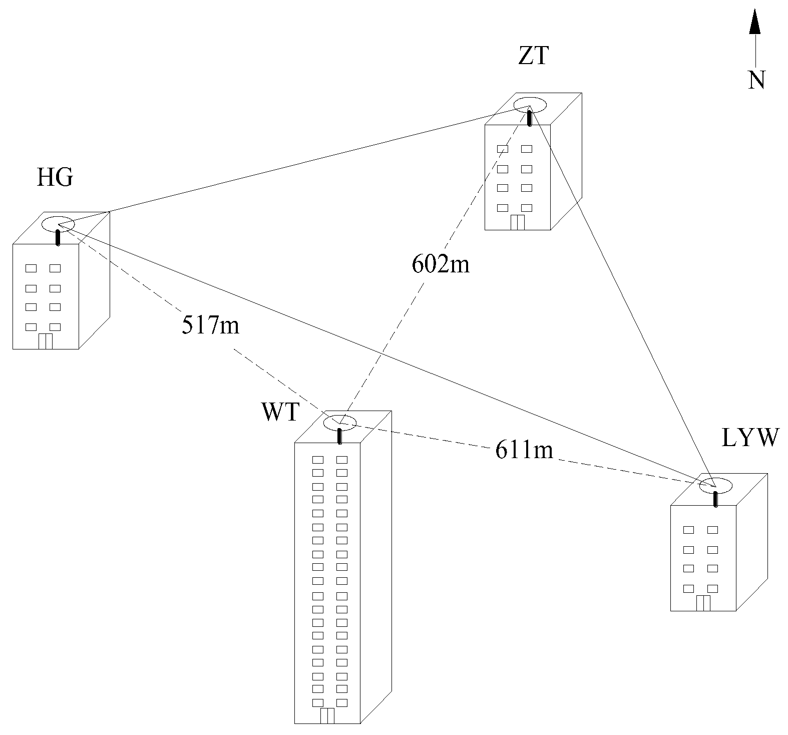
The authors chose point WT (W Tower, the average of the plumbing points) as the monitoring station on the roof of the W Tower. In order to reduce the impact of the W Tower’s motion on the vertical reference transmission, the reference point is first transmitted by the laser plummet at different moments. Then, the authors chose the average of plumbing points as the monitoring point WT. In addition, three points (HG, LYW, and ZT) are chosen from five construction control points to establish a reference network around the W Tower as shown in Figure 6. The authors chose these locations based on their suitability as reference stations according to the International GNSS service (IGS) criteria, keeping in mind the difficulty of finding adequate locations in an urban setting. Three control points were located on the concrete buildings as low as 100 m. Dual-frequency Trimble R8 GNSS receivers were placed at all stations to collect 24 h and 23 min data with a sampling rate of 0.067 Hz.
The GNSS data of the reference network consisting of points HG, ZT, and LYW was firstly processed in the static mode to obtain the baseline vectors between reference stations. Secondly, the GNSS data of the monitoring station, namely WT, was processed in the post-processed kinematic mode to obtain baseline vectors from the monitoring station to each reference station, giving a total of 13,495 baseline vectors at 5648 epochs. Among others, there are 659 single baselines, which means only one baseline vector can be successfully calculated between the monitoring station and one of the three reference stations at 659 epochs. In particular, the 659 baseline vectors will be used directly without any processing in the following. Owing to observational conditions, the integer ambiguity resolution cannot be fixed at 206 epochs. Thirdly, the monitoring network was constructed by the reference network and the baseline vectors between the monitoring station and reference stations at each epoch. Then, the authors check the misclosures and the corrections of baseline vectors to identify and eliminate gross errors of baseline vectors epoch-by-epoch. By checking the misclosures and the corrections of baseline vectors, total of 1726 baseline vectors are eliminated as gross errors. Referring to the statistics listed in Table 5, after processing, the corrections of all baseline vectors are less than 3 times the standard deviation σ of the baseline vector, and 96.27%, 91.59%, and 98.03% of corrections are within the range of ±2.0 cm for all three directions (not including the 659 single baseline vectors).
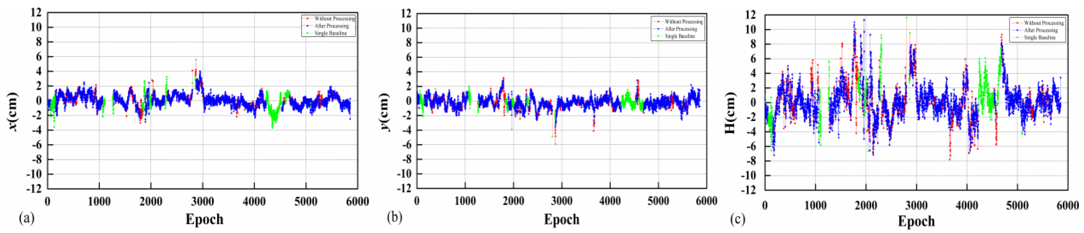
Finally, the reference points’ coordinates can be used as a constraint to then process the GNSS monitoring network via a least-squares adjustment at each epoch. Table 6 lists the statistics of the differences in position with respect to the coordinate time series of the monitoring point as shown in Figure 7 in the x, y, and H directions without and with processing.
Referring to the statistics listed in Table 6, one may see that a small number of gross errors have been eliminated, especially in the x and y directions. After processing, the differences of 96.48% of the x coordinates and 98.57% of the y coordinates are within ±2.0 cm, while the differences of 90.49% of the H coordinates is within ±4.0 cm. However, there are some abnormal coordinates included in the result above (shown by the green points in Figure 7), which are calculated by just one reference point and one baseline vector instead of using a least-squares adjustment. In addition, the operation of a tower crane has an impact on the motion of the W Tower.
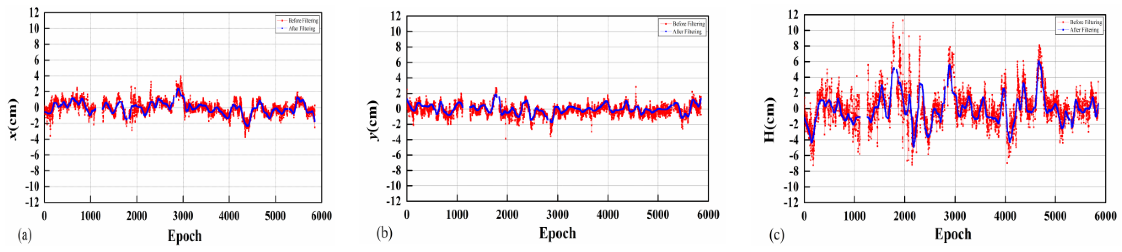
Nevertheless, the coordinate time series of the monitoring point contain both the displacement information and the measurement-error information after the aforementioned processing. The displacement of the monitoring point is characterized by a systematic signal even though it may be small over a short time period, but the measurement-error is characterized by strong noise that can be removed by wavelet filtering [29,30]. In order to extract the displacement signal of the W Tower, the wavelet filter is applied to further process the coordinate time series. Based on the understanding of the signal as discussed previously, a db4 wavelet filter at level 6 is applied to eliminate the background noise hidden in the coordinate time series. Figure 8 shows the coordinate variations before and after filtering.
The standard deviations (STDs) of the background noises are ±5.0, ±4.5, and ±13.0 mm in the x, y, and H directions, respectively. It is evident that, after the filtering, the background noises are almost eliminated and the GNSS time-series becomes smoother. After filtering, the differences of 89.34% of the x coordinates and 95.08% of the y coordinates are within ±1.0 cm, while the differences of 95.24% of the H coordinates are within ±4.0 cm. In addition, the results show that the displacement in the x direction is slightly larger than the displacement in the y direction, which may be related to wind direction. Therefore, one may conclude that the displacement of the W Tower is within ±1.0 cm in horizontal direction at most epochs, so it has less impact on the vertical reference transmission.
5.2. Calculating Deflection of the Vertical Components for the Monitoring Point
Now, let us calculate the deflection of the vertical components using the Earth gravity field model and the GZGEOID model [32]. EGM2008 (to degree 2160) and EIGEN-6C4 (to degree 2190) (http://icgem.gfz-potsdam.de/) were used to calculate deflections of the vertical by Equations (8) and (9). Qi et al. have estimated the accuracy of the EGM2008 model with 466 first-order astrogeodetic points in the east (>102° E) of China. The estimated accuracy of deflection of the vertical components from the EGM2008 model are ±1.734′′ and ±1.649′′ in the north-south and east-west components, respectively [33], which is main reason for selecting the EGM2008 and EIGEN-6C4 (including GOCE(Gravity field and steady-state Ocean Circulation Explorer) data) models.
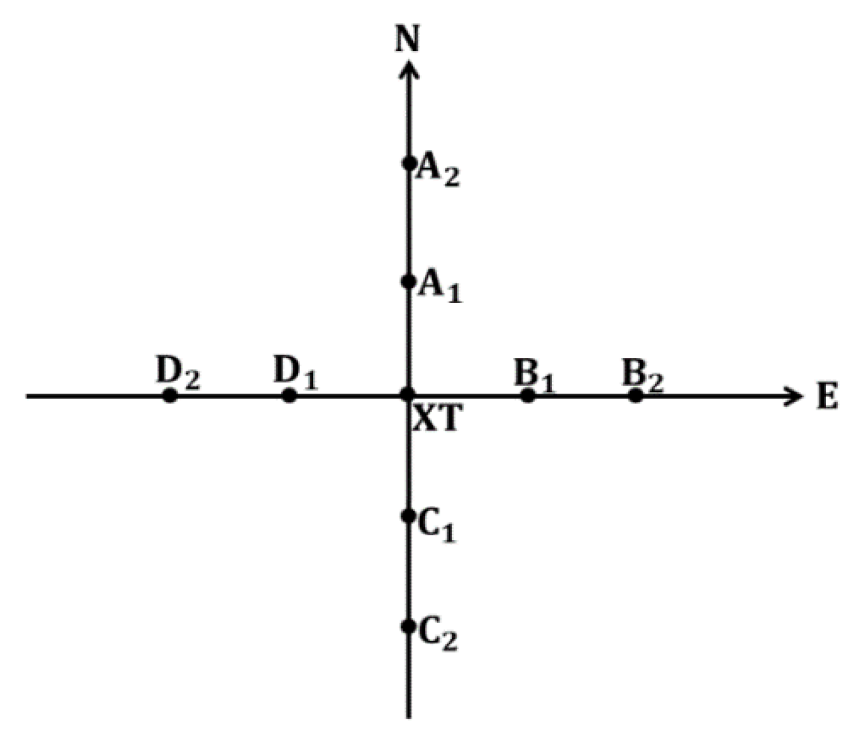
Considering and [32], and assuming that orthometric height differences and ellipsoidal height differences are not correlated, we obtain . If the accuracy of the deflection of the vertical components is expected to be about 1 arc second, the is about 1.6 km according to Equation (11). Finally, eight points along the north-south (A2, A1, C1, and C2) and east-west (B2, B1, D1, and D2) directions are chosen to calculate the deflection of the vertical components (see Figure 9), The distances from A1, B1, C1, and D1 to XT are about 30 arc seconds, and the distances from A2, B2, C2, and D2 to XT are about 60 arc seconds. The geoid height difference can be calculated from the GZGEOID model and the EGM2008 and EIGEN-6C4 gravity field models, respectively, and we can obtain the deflection of the vertical components according to Equation (10). The results are shown in Table 7. The Table 7 shows that the results from the GZGEOID, EGM2008, and EIGEN-6C4 models have good consistency. The average deflection of the vertical components from the GZGEOID, EGEM2008, and EIGEN-6C4 models are shown in Table 8, respectively. For instance, the deflection of the vertical component ξ from GZGEOID is the average of 3.80″, 4.25″, 3.91″, and 4.36″, and the deflection of the vertical component η from GZGEOID is the average of −6.04″, −5.80″, −6.04″, and −5.80″, and so on.
5.3. Verticality Monitoring Result of the W Tower
In order to validate/check the result of laser plumbing by comparison with the GNSS result, the GNSS data of the monitoring network consisting of points HG, ZT, LYW, and WT were reprocessed in static mode to obtain the mean coordinate of WT. Then, the systematic bias between the coordinates of a GNSS measurement and a laser plumbing measurement can be calculated by Equations (12) and (13) with the ellipsoidal height of the monitoring point (hWT = 432.477 m) and the deflection of the vertical components. Table 8 lists the corresponding corrections of the plane coordinates of the monitoring point (WT). The differences between the coordinates of the laser plumbing and GNSS measurements without corrections are listed in Table 9.
The coordinates of the GNSS measurement can be corrected with the corrections listed in Table 8. The differences between the coordinates of the laser plumbing and GNSS measurements with corrections are listed in Table 10.
In the x direction, it can be seen that the difference between the coordinates of the GNSS measurement and the laser plumbing measurement has been reduced by the corrections calculated with the deflections of the vertical. However, in the y direction, it seems that the corrected difference becomes worse. In fact, there are two possibilities. On one hand, the accuracy of deflections of the vertical leads to the results, with a building height of 432 m, when the accuracy of deflections of the vertical is about 1–2 arc seconds, which may lead to a difference of millimeters. On the other hand, the corrected difference may be the actual difference caused by construction and measurement errors. As shown in Table 10, the difference in position between the GNSS measurement and the laser plumbing measurement is within 2.0 cm after correction. Therefore, when considering such factors as the wind, the operation of a tower crane, and the installation of a curtain wall, one may conclude that the verticality of the W Tower is within 2.0 cm.
6. Conclusions
This paper aims to monitor the verticality and analyze the horizontal motion of the W Tower in Guangzhou, China via GNSS technology, from which the following conclusions were drawn:
- The data processing strategy for calculating the monitoring point’s coordinate time series and deflections of the vertical are introduced. The 24-h observation result shows that the displacement variations of the W Tower are within ±1.0 cm in the horizontal direction at most epochs, so it has less impact on the vertical reference transmission of the W Tower.
- Comparison shows that deflections of the vertical calculated by the Earth gravity field model (e.g., EGM2008) were also very close to that calculated by the GZGEOID model. The high-precision deflection of the vertical components play an important role in matching the results of the GNSS measurement and laser plumbing measurement. When considering such factors as the wind, the operation of a tower crane, and the installation of a curtain wall, one may conclude that the verticality of the W Tower is within the range of 2.0 cm after correction, which meets the design requirement of ±3.0 cm according to the Technical Specification for Concrete Structures of Tall Buildings in China.
Author Contributions
X.Z. and Y.Z. did the measurements, data processing, and contributed to the writing. B.L. and G.Q. contributed to the revisions and discussions of the contents.
Funding
This research was funded by National Natural Science Foundation of China grant number NSFC 41674006, 41731069.
Acknowledgments
We acknowledge the valuable comments by Professor Gerard Lachapelle and three other anonymous reviewers.
Conflicts of Interest
The authors declare no conflict of interest.
References
- Hudnut, K.W.; Behr, J. A continuous GPS monitoring of structural deformation at Pacoima Dam, California. Seismol. Res. Lett. 1998, 69, 299–308. [Google Scholar] [CrossRef]
- He, X.; Yang, G.; Ding, X.; Chen, Y. Application and evaluation of a GPS multi-antenna system for dam deformation monitoring. Earth Planets Space 2004, 56, 1035–1039. [Google Scholar] [CrossRef] [Green Version]
- Rutledge, D.R.; Meyerholtz, S.Z.; Brown, N.; Baldwin, C. Dam stability: Assessing the performance of a GPS monitoring system. GPS World 2006, 17, 26–33. [Google Scholar]
- Li, W.; Wang, C. GPS in the tailings dam deformation monitoring. Procedia Eng. 2011, 26, 1648–1657. [Google Scholar] [CrossRef]
- Meng, X.; Dodson, A.H.; Roberts, G.W. Detecting bridge dynamics with GPS and triaxial accelerometers. Eng. Struct. 2007, 29, 3178–3184. [Google Scholar] [CrossRef]
- Moschas, F.; Stiros, S. Measurement of the dynamic displacements and of the modal frequencies of a short-span pedestrian bridge using GPS and an accelerometer. Eng. Struct. 2011, 33, 10–17. [Google Scholar] [CrossRef]
- Kaloop, M.R.; Kim, D. GPS-structural health monitoring of a long span bridge using neural network adaptive filter. Surv. Rev. 2014, 334, 7–14. [Google Scholar] [CrossRef]
- Kumberg, T.; Schneid, S.; Reindl, L. A Wireless Sensor Network Using GNSS Receivers for a Short-Term assessment of the Modal Properties of the Neckartal Bridge. Appl. Sci. 2017, 7, 626. [Google Scholar] [CrossRef]
- Yi, T.H.; Li, H.N.; Gu, M. Experimental assessment of high-rate GPS receivers for deformation monitoring of bridge. Measurement 2013, 46, 420–432. [Google Scholar] [CrossRef]
- Lovse, J.W.; Teskey, W.F.; Lachapelle, G.; Cannon, M.E. Dynamic Deformation Monitoring of a Tall Structure Using GPS Technology. J. Surv. Eng. 1995, 121, 35–40. [Google Scholar] [CrossRef]
- Tamura, Y.; Matsui, M.; Pagnini, L.C.; Ishibashi, R.; Yoshida, A. Measurement of wind-induced response of buildings using RTK-GPS. J. Wind Eng. Ind. Aerodyn. 2002, 90, 1783–1793. [Google Scholar] [CrossRef] [Green Version]
- Casciati, F.; Fuggini, C. Monitoring a steel building using GPS sensors. Smart Struct. Syst. 2011, 7, 349–363. [Google Scholar] [CrossRef]
- Yi, J.; Zhang, J.W.; Li, Q.S. Dynamic characteristics and wind-induced responses of a super-tall building during typhoons. J. Wind Eng. Ind. Aerodyn. 2013, 121, 116–130. [Google Scholar] [CrossRef]
- Tang, X.; Roberts, G.W.; Li, X.; Hancock, C.M. Real-time Kinematic PPP GPS for Structure Monitoring Applied on the Severn Suspension Bridge, UK. Adv. Space Res. 2017, 60, 925–937. [Google Scholar] [CrossRef]
- Sampietro, D.; Caldera, S.; Capponi, M.; Realini, E. Geoguard-An Innovative Technology Based on Low-cost GNSS Receivers to Monitor Surface Deformations. In Proceedings of the First EAGE Workshop on Practical Reservoir Monitoring, Amsterdam, The Netherlands, 6–9 March 2017. [Google Scholar]
- Chan, W.S.; Xu, Y.L.; Ding, X.L.; Dai, W.J. An integrated GPS–accelerometer data processing technique for structural deformation monitoring. J. Geod. 2006, 80, 705–719. [Google Scholar] [CrossRef]
- Li, X.; Ge, L.; Ambikairajah, E.; Rizos, C.; Tamura, Y.; Yoshida, A. Full-scale structural monitoring using an integrated GPS and accelerometer system. GPS Solut. 2006, 10, 233–247. [Google Scholar] [CrossRef]
- Quesada-Olmo, N.; Jimenez-Martinez, M.J.; Farjas-Abadia, M. Real-time high-rise building monitoring system using global navigation satellite system technolog. Measurement 2018, 123, 115–124. [Google Scholar] [CrossRef]
- Im, S.B.; Hurlebaus, S.; Kang, Y.J. Summary review of GPS technology for structural health monitoring. J. Struct. Eng. 2011, 10, 1653–1664. [Google Scholar] [CrossRef]
- Driving Vertical Towers. Available online: https://www.gim-international.com/ content/article/ driving- vertical-towers (accessed on 28 June 2010).
- Lachapelle, G.; Dennler, M.; Lethaby, J.; Cannon, M.E. Special order geodetic operations for a canadian pacific railway tunnel in the canadian rockies. Can. Surv. 1984, 38, 163–176. [Google Scholar]
- Hirt, C.; Seeber, G. Accuracy analysis of vertical deflection data observed with the hannover digital zenith camera system TZK2-D. J. Geod. 2008, 82, 347–356. [Google Scholar] [CrossRef]
- Wang, Y.M.; Becker, C.; Mader, G.; Martin, D.; Li, X.; Jiang, T.; Breidenbach, S.; Geoghegan, C.; Winester, D.; Guillaume, S.; et al. The Geoid slope validation survey 2014 and GRAV-D airborne gravity enhanced geoid comparison results in Iowa. J. Geod. 2017, 91, 1261–1276. [Google Scholar] [CrossRef]
- Jekeli, C. An analysis of vertical deflections derived from high-degree spherical harmonic models. J. Geod. 1999, 73, 10–22. [Google Scholar] [CrossRef]
- Hirt, C. Efficient and accurate high-degree spherical harmonic synthesis of gravity field functionals at the Earth’s surface using the gradient approach. J. Geod. 2012, 86, 729–744. [Google Scholar] [CrossRef]
- Tse, C.M.; Baki Iz, H. Deflection of the vertical components from GPS and precise leveling measurements in Hong Kong. J. Surv. Eng. 2006, 132, 97–100. [Google Scholar] [CrossRef]
- Ceylan, A. Determination of the deflection of vertical components via GPS and leveling measurement: A case study of a GPS test network in konya, turkey. Sci. Res. Essays 2010, 4, 1438–1444. [Google Scholar]
- Liu, D.; Bai, Z.; Shi, Y.; Shen, Y. Geodetic Coordinate Transformation, GPS Control Network Adjustment and Software System; Tongji University Press: Shanghai, China, 1997. [Google Scholar]
- Kaloop, M.R.; Li, H. Sensitivity and analysis GPS signals based bridge damage using GPS observations and wavelet transform. Measurement 2011, 44, 927–937. [Google Scholar] [CrossRef]
- Kumar, K.V.; Miyashita, K.; Li, J. Secular crustal deformation in central Japan, based on the wavelet analysis of GPS time-series data. Earth Planets Space 2002, 54, 133–139. [Google Scholar] [CrossRef] [Green Version]
- Pavlis, N.K.; Holmes, S.A.; Kenyon, S.C.; Factor, J.K. The development and evaluation of the Earth Gravitational Model 2008 (EGM2008). J. Geophys. Res. Solid Earth 2012, 117, B04406. [Google Scholar] [CrossRef]
- Yang, G.; Lin, H.; Ou, H.; Fang, F.; Li, J. Quasi-geoid Determination with Sub-centimeter Precision in City Guangzhou. Bull. Surv. Mapp. 2007, 1, 24–25. [Google Scholar]
- Qi, X.; Zhou, W.; Cui, J. Accuracy Analysis of EGM2008 Model based on Vertical Deflection in China. Geom. Technol. Equip. 2011, 13, 6–8. [Google Scholar]
Figure 1.
Schematic of plumbing with a laser plummet.

Figure 2.
The flowchart diagram for calculating the monitoring point’s coordinate time series.

Figure 3.
Difference between the Global Navigation Satellite System (GNSS) measurement and laser plumbing. (a) The relationship between plumb line and ellipsoid normal during monitoring; (b) Decomposition of the deflection of the vertical u.
Figure 3.
Difference between the Global Navigation Satellite System (GNSS) measurement and laser plumbing. (a) The relationship between plumb line and ellipsoid normal during monitoring; (b) Decomposition of the deflection of the vertical u.

Figure 4.
GNSS monitoring network in simulation.

Figure 5.
Differences in position in relation to the coordinate time series of the monitoring point: (a) x direction; (b) y direction; (c) H direction.
Figure 5.
Differences in position in relation to the coordinate time series of the monitoring point: (a) x direction; (b) y direction; (c) H direction.

Figure 6.
GNSS monitoring network.

Figure 7.
Differences in position in relation to the coordinate time series of the monitoring point: (a) x direction; (b) y direction; (c) H direction.
Figure 7.
Differences in position in relation to the coordinate time series of the monitoring point: (a) x direction; (b) y direction; (c) H direction.

Figure 8.
Differences in position in relation to the coordinate time series of the monitoring point: (a) x direction; (b) y direction; (c) H direction.
Figure 8.
Differences in position in relation to the coordinate time series of the monitoring point: (a) x direction; (b) y direction; (c) H direction.

Figure 9.
Distribution of Points for calculating the deflections of the vertical components.


Table 1.
Approximations of the systematic bias at different building heights.
| Building Height (m) | Δx (mm) | Δy (mm) |
|---|---|---|
| 100 | −1.6 | +3.2 |
| 200 | −3.2 | +6.4 |
| 300 | −4.7 | +9.6 |
| 400 | −6.3 | +12.8 |
Table 2.
Statistics of misclosures of the spatial GNSS monitoring network (%).
| XYZ Directions | xyH Directions | |||||
|---|---|---|---|---|---|---|
| wX | wY | wZ | wx | wy | wH | |
| <1 cm | 71.38 | 39.51 | 76.79 | 94.51 | 70.99 | 38.23 |
| 1–2 cm | 26.26 | 31.34 | 20.27 | 5.35 | 26.39 | 30.18 |
| 2–3 cm | 2.21 | 17.96 | 2.78 | 0.13 | 2.49 | 18.02 |
| 3–4 cm | 0.14 | 7.63 | 0.12 | 0.01 | 0.13 | 8.50 |
| 4–5.2 cm | 0.01 | 2.30 | 0.02 | 0 | 0 | 3.16 |
| ≥5.2 cm | 0 | 1.26 | 0.02 | 0 | 0 | 1.91 |
Table 3.
Statistics of baseline vectors’ corrections of the spatial GNSS monitoring network (%).
| Before Processing | After Processing | |||||
|---|---|---|---|---|---|---|
| VΔX | VΔY | VΔZ | VΔX | VΔY | VΔZ | |
| <1 cm | 93.79 | 64.38 | 93.09 | 94.19 | 65.27 | 94.20 |
| 1–2 cm | 6.16 | 27.37 | 6.62 | 5.78 | 28.08 | 5.76 |
| 2–3 cm | 0.05 | 6.54 | 0.29 | 0.03 | 6.65 | 0.04 |
| ≥3 cm | 0 | 1.71 | 0 | 0 | 0 | 0 |
Table 4.
Statistics of differences in position in relation to the coordinate time series of the monitoring point (%).
Table 4.
Statistics of differences in position in relation to the coordinate time series of the monitoring point (%).
| xyH Direction (without Processing) | xyH Directions (after Processing) | |||||
|---|---|---|---|---|---|---|
| Vx | Vy | VH | Vx | Vy | VH | |
| <0.5 cm | 89.01 | 61.12 | 19.56 | 89.26 | 61.12 | 20.26 |
| 0.5–1 cm | 10.94 | 34.13 | 19.54 | 10.74 | 34.24 | 20.45 |
| 1–2 cm | 0.05 | 4.71 | 35.36 | 0 | 4.64 | 36.60 |
| 2–3 cm | 0 | 0.04 | 17.88 | 0 | 0 | 16.87 |
| ≥3 cm | 0 | 0 | 7.66 | 0 | 0 | 5.82 |
Table 5.
Statistics of baseline vectors’ corrections of the spatial GNSS monitoring network (%).
| Before Processing | After Processing | |||||
|---|---|---|---|---|---|---|
| VΔX | VΔY | VΔZ | VΔX | VΔY | VΔZ | |
| <1 cm | 78.81 | 63.38 | 80.17 | 80.64 | 65.27 | 82.08 |
| 1–2 cm | 15.46 | 25.32 | 16.42 | 15.63 | 26.32 | 15.95 |
| 2–3 cm | 3.81 | 8.40 | 2.94 | 3.73 | 8.41 | 1.97 |
| ≥3 cm | 1.92 | 2.90 | 0.47 | 0 | 0 | 0 |
Table 6.
Statistics of differences in position in relation to the coordinate time series of the monitoring point (%).
Table 6.
Statistics of differences in position in relation to the coordinate time series of the monitoring point (%).
| xyH Directions (without Processing) | xyH Directions (after Processing) | |||||
|---|---|---|---|---|---|---|
| Vx | Vy | VH | Vx | Vy | VH | |
| <1 cm | 76.14 | 82.39 | 40.05 | 76.63 | 84.05 | 41.50 |
| 1–2 cm cm | 20.18 | 15.68 | 27.31 | 19.85 | 14.52 | 27.27 |
| 2–3 cm | 3.03 | 1.54 | 14.48 | 2.98 | 1.28 | 14.91 |
| 3–4 cm | 0.60 | 0.28 | 7.56 | 0.54 | 0.15 | 6.81 |
| ≥4 cm | 0.05 | 0.11 | 10.60 | 0 | 0 | 9.51 |
Table 7.
The deflection of vertical components from the GZGEOID, EGM2008, and EIGEN-6C4 models.
| From | To | GZGEOID | EGM2008 | EIGEN-6C4 | |||
|---|---|---|---|---|---|---|---|
| ΔN/m | ξ/η(″) | ΔN/m | ξ/η(″) | ΔN/m | ξ/η(″) | ||
| XT | A1 | −0.018 | 3.80 | −0.014 | 3.20 | −0.013 | 2.99 |
| C1 | 0.019 | 4.25 | 0.014 | 3.21 | 0.013 | 2.99 | |
| B1 | 0.025 | −6.04 | 0.028 | −6.65 | 0.028 | −6.69 | |
| D1 | −0.024 | −5.80 | −0.027 | −6.57 | −0.027 | −6.64 | |
| A2 | −0.035 | 3.91 | −0.029 | 3.21 | −0.027 | 3.00 | |
| C2 | 0.038 | 4.36 | 0.029 | 3.23 | 0.027 | 3.01 | |
| B2 | 0.050 | −6.04 | 0.055 | −6.69 | 0.056 | −6.73 | |
| D2 | −0.048 | −5.80 | −0.054 | −6.53 | −0.054 | −6.56 | |
Table 8.
The vertical deflections and the corrections of plane coordinates calculated with different strategies.
Table 8.
The vertical deflections and the corrections of plane coordinates calculated with different strategies.
| Method | ξ (″) | η (″) | Δx (mm) | Δy (mm) |
|---|---|---|---|---|
| EGM2008 | +3.21 | −6.617 | −6.7 | +13.9 |
| EIGEN-6C4 | +3.00 | −6.667 | −6.3 | +14.0 |
| GZGEOID | +4.08 | −5.924 | −8.6 | +12.4 |
Table 9.
Differences between the coordinates of the laser plumbing and GNSS measurements (m).
| Laser Plumbing | GNSS Measurement | Differences | |||||
|---|---|---|---|---|---|---|---|
| x | y | x | y | x Direction | y Direction | xy Directions | |
| WT | 8258.284 | 3535.986 | 8258.310 | 3535.976 | +0.026 | −0.010 | 0.028 |
Table 10.
Differences between the coordinates of the laser plumbing and GNSS measurements after correction (mm).
Table 10.
Differences between the coordinates of the laser plumbing and GNSS measurements after correction (mm).
| Method | x Direction | y Direction | xy Directions |
|---|---|---|---|
| EGM2008 | +19.3 | +3.9 | 19.5 |
| EIGEN-6C4 | +19.7 | +4.0 | 20.1 |
| GZGEOID | +17.4 | +2.4 | 17.6 |
© 2018 by the authors. Licensee MDPI, Basel, Switzerland. This article is an open access article distributed under the terms and conditions of the Creative Commons Attribution (CC BY) license (http://creativecommons.org/licenses/by/4.0/).
Share and Cite
MDPI and ACS Style
Zhang, X.; Zhang, Y.; Li, B.; Qiu, G. GNSS-Based Verticality Monitoring of Super-Tall Buildings. Appl. Sci. 2018, 8, 991. https://doi.org/10.3390/app8060991
AMA Style
Zhang X, Zhang Y, Li B, Qiu G. GNSS-Based Verticality Monitoring of Super-Tall Buildings. Applied Sciences. 2018; 8(6):991. https://doi.org/10.3390/app8060991
Chicago/Turabian StyleZhang, Xingfu, Yongyi Zhang, Bofeng Li, and Guangxin Qiu. 2018. "GNSS-Based Verticality Monitoring of Super-Tall Buildings" Applied Sciences 8, no. 6: 991. https://doi.org/10.3390/app8060991
Note that from the first issue of 2016, this journal uses article numbers instead of page numbers. See further details here.