A Novel Approach for Outdoor Fall Detection Using Multidimensional Features from A Single Camera

Abstract

In the past few years, it has become increasingly important to automatically detect falls and provide feedback in emergency situations. To meet these demands, fall detection studies have been undertaken using various methods ranging from wearable devices to vision-based methods. However, each method has its own limitations and one common limitation that is prevalent in almost all fall detection studies is that they are restricted to indoor environments. Therefore, we focused on a more dynamic and complex outdoor environment. We used two-dimensional features and Rao-Blackwellized Particle Filtering for human detection and tracking, and extracted three-dimensional features from depth images estimated by the supervised learning method from single input images. As we used the methods in combination, we could distinguish a series of states in which a person falls more precisely and then successfully perform fall detection under dynamic and complex scenes. In this study, we solved the initialization problem, the main constraint of existing tracking studies, by applying the particle swarm optimization method to the human detection system. In addition, we avoided using the background reference image feature for image segmentation due to its vulnerability towards dynamic outdoor changes. The experimental results show a reliable and robust performance for the proposed method and suggest the possibility of effective application to the pre-existing surveillance systems.

1. Introduction

With the continuous aging of the global population, there has been an alarming increase in the number of incidents of the elderly falling that cause severe injuries and sometimes even death. According to the World Health Organization in [1], 28–35% of people aged 65 or more encounter falls and the incident rate is even higher for people aged 70 or above. Falls can be potentially fatal in cases when an elder is alone. This is resulting in a steady increase in the social costs involving pre-incident preventive measures and post-incident treatments. Hence, multiple recent studies that have been undertaken aim to develop an intelligent solution that automatically detects falls and raises an emergency alert targeted to an elderly person who lives alone. However, no perfect solution has been developed to date due to challenges, such as non-deterministic fall patterns and the illumination factor.

The most recent fall detection studies are based on wearable, ambience, or vision sensors [2]. The wearable device-based fall detection system uses accelerometers, gyroscopes, or other body sensors embedded in garments [3,4,5,6,7]. The wearable sensor-based fall detection methods uncover changes in a human body through wearable sensors attached to the body. This method is simple, computationally efficient, and easy to install. However, as several kinds of sensors need to be physically attached to the body, such a wearable sensor-based fall detection system proves to be slightly inconvenient to the users. In addition, it needs periodic replacement of batteries that power it and may have side effects due to a lasting exposure to electromagnetic waves. Although the accuracy of alarms can be improved by fusing different sensors [8,9], such a conjugated method often leads to inconvenience. An ambience-based fall detection system typically uses vibration sensors, infrared (IR) sensors, pressure sensors, and several other devices that can be used individually or in combination to detect the position and abnormality of a person to trigger a fall alarm [10,11,12,13,14]. Unlike a wearable sensor-based fall detection method, the ambience-based fall detection system is a non-invasive method, however there are many false alarms. Moreover, it is difficult to use this system comprehensively in indoor or outdoor environments because a fall can only be detected in an area that is equipped with sensors.

With new advancements in computer vision research, diverse vision-based fall detection systems are being studied. Such vision-based fall detection systems can be classified into three main categories: single camera-based fall detection systems, multi-camera-based fall detection systems, and depth camera-based fall detection systems. In general, numerous single camera-based fall detection systems extract an individual’s silhouette by adopting a background model (e.g., a background reference image). From the individual silhouette, various features such as the width and the length of a bounding box, the ellipse aspect ratio of the orientation, and edges are used to detect a fall [15,16,17]. However, the constantly and dynamically changing background of recorded scenes due to illumination and the presence of shadows in outdoor environments causes a lot of errors. Moreover, the aspect ratio of a bounding box or an ellipse, commonly used for human tracking with 2D images, is not sufficient to detect a fall accurately.

More specifically, some studies [18,19] related to single camera cases tried to detect falls based on the motion contour by analyzing the motion energy or using the integrated spatiotemporal energy map. However, the fact that the analysis of motion energy varies from person to person makes it difficult to be used for general cases. In addition, a single camera is not capable of providing 3D information required for a robust fall detection. To overcome this limitation, another fall detection study brings forth the possibility of using estimated 3D head motions with a single camera [20], but the system works only with a pre-calibrated camera and an initialized head position. These facts indicate that fall detection systems based on a single camera have their own drawbacks.

The fall detection systems based on multiple cameras can track 3D motions using 3D reconstruction of foreground objects [21,22], but the calibration of multiple cameras is problematic and causes computational complexity. Moreover, the need for additional cameras increases the cost and gives rise to various hassles in an outdoor environment. Recently, multiple studies have been conducted using kinetic cameras or depth sensors [23,24,25,26]. These sensors generate accurate depth images in real-time that improve the performance of human detection and tracking in the 3D space. However, this approach increases the additional cost for existing surveillance systems. Moreover, a depth camera does not work accurately in an outdoor environment and there are restrictions in terms of distance [27]. In most vision-based fall detection studies conducted to a date, the focus has been to automatically detect falls of the elderly in the indoor environment. Fall detection in an outdoor environment is more difficult since human motion and surrounding scenarios are more dynamic and complex in general, as compared to the indoor environment. Nonetheless, there has been very little research on noninvasive methods, which is our research direction. It is different from the few studies conducted on the effectiveness of using wearable sensors [28,29,30].

In this study, we propose a single camera-based fall detection method to be used in an outdoor environment. In spite of using a single camera, this approach employs 3D movement by analyzing depth images estimated by a machine learning algorithm. Furthermore, our study presents the possibility of outdoor fall detection which is not a well-studied topic yet. To summarize the process, first, a depth image is generated from an input image captured by a RGB camera and then a global optimization method is applied to detect a human form in the depth image. Our method does not employ the initialization process generally required for human tracking in other methods. After a human form is detected, prediction and update steps are performed continuously to track the detected human form using a particle filter. The measurement information used in the update process is computed by applying the graph-cut method. This rules out the need of the background subtraction method (i.e., no use of background reference image), which is frequently used in other detection methods. Therefore, we can say that this approach facilitates the use of existing surveillance systems and provides a novel and universal fall detection method that enables fall detection in various outdoor environments.

In the subsequent sections, we introduce the methods used and present the proposed method in Section 2, show our experimental results in Section 3, and present the conclusions in Section 4.

2. Materials and Methods

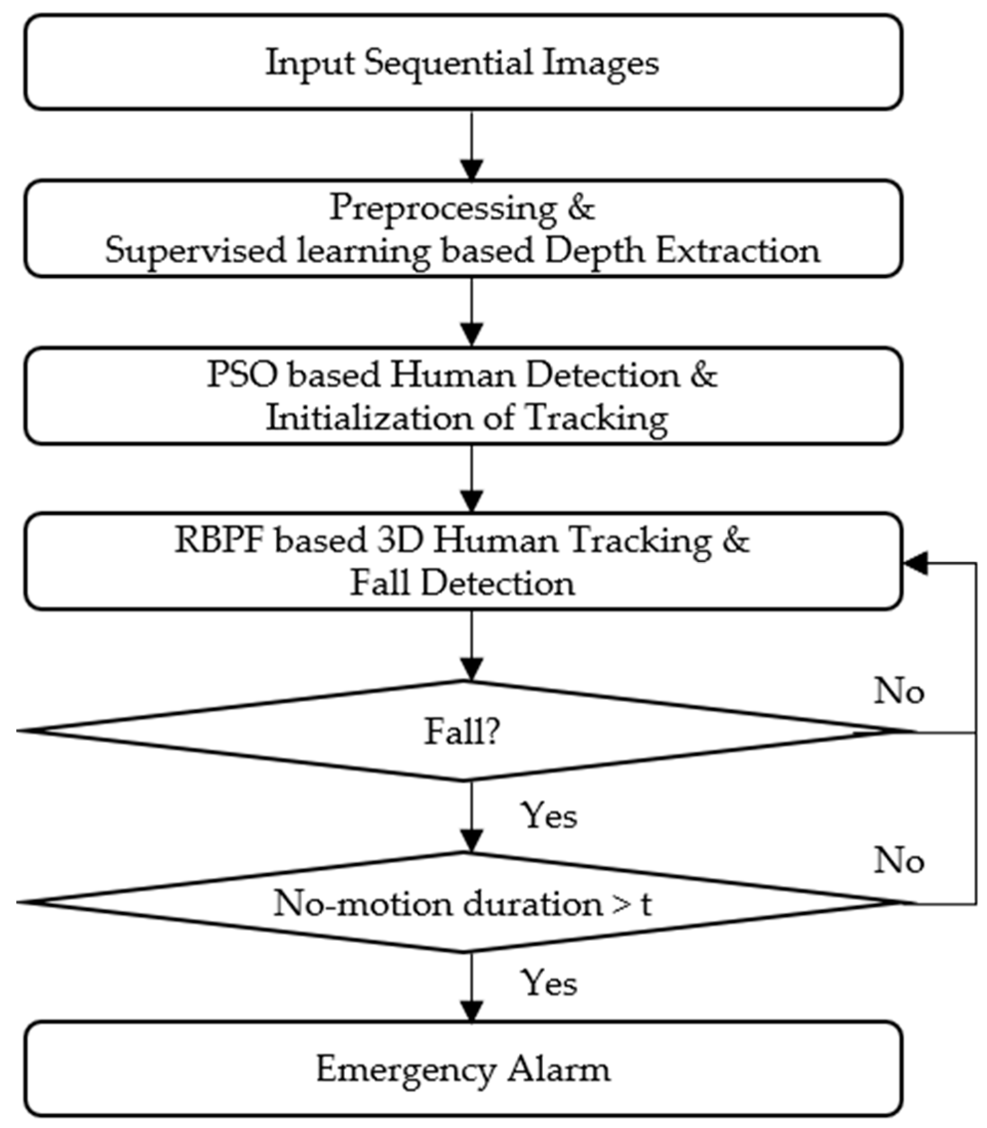
Figure 1 shows the overall algorithm proposed in our study. When an image is received, the algorithm converts the RGB color space into a HSV color space and applies histogram equalization to the input image. This preprocessing alleviates the sensitivity to illumination changes [31]. A depth image is then generated from the input image using a supervised learning technique. In the depth image, a human form is represented as a cluster area having the same or similar depth, which makes it easy to detect shapes and locations of the human. To automatically detect a human form and initialize tracking, we use a global optimization method called particle swarm optimization (PSO) that calculates the optimum size of a bounding box (window) enclosing the human and the box location simultaneously. This information serves as the input for the foreground (inside) and background (outside) information of the graph-cuts method, which helps detect a person and initialize the parameters of an ellipse model, thus enclosing the human to be tracked. In the next step, the ellipse (human) is tracked through iterative predictions and update steps of the Rao-Blackwellized Particle Filter (RBPF). While tracking, our fall detection algorithm determines whether a fall occurs or not by analyzing both 2D and 3D features of the ellipse model (human). Once the algorithm detects a fall, our system raises an emergency alarm in case the duration of the subsequent no-motion phase is prolonged. In the following flowchart, each step of the algorithm is explained.

2.1. Supervised Learning Based Depth Extraction

Assuming that a general depth image is obtained through multiple cameras, a learning method needs to be developed to obtain depth images using a single camera. In this study, we use the depth estimation method introduced by [32]. The depth image of the input image is built by training various monocular images taken in indoor and outdoor environments along with ground truth depth images measured by the laser scanner. A depth image is derived from a discriminatively trained Markov Random Field (MRF) for local and global features in combination with the individual and relative depths that denote the depths between different points. Here we derive a depth image for a new input image based on a training set that is composed of 425 individual images and depth image pairs. The trained image resolution is 1704 × 2272 and depth image resolution is 86 × 107. The trained images are of objects that we often encounter, such as forest, trees, buildings, roads, sidewalks, and so on.

Depth Estimation from Both Absolute Depth and Relative Depth Features

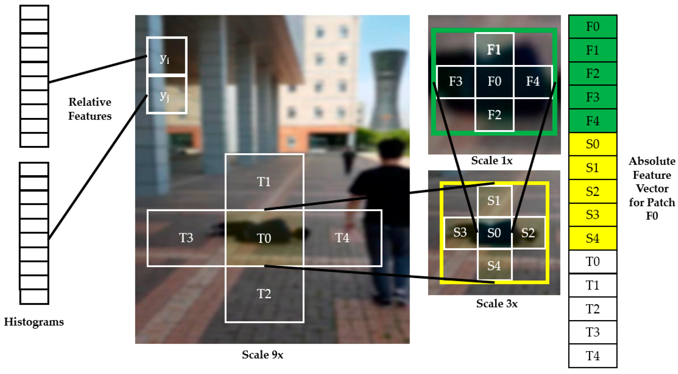
Two types of features, absolute and relative depth features, are required for each patch (e.g., T0–T4 in Figure 2) to estimate the scene global depth from a single image as seen in Figure 2. The entire process can be summarized as follows. First, a feature vector (E_i(n)) for a patch is obtained through the Equation (1) with a predefined filter F for the input image. Second, based on the feature vector, the absolute depth features are computed with multiple spatial scales of the patch and its surrounding patches as seen in the right-side of Figure 2. For instance, F0–F4, S0–S4, T0–T4 in Figure 2 are absolute feature vectors obtained with different scales from a patch F0. Third, the relative depth features are computed by the difference of the histograms (|y_i − y_j|) from each patch (y_i and y_j in Figure 2) on the left-hand side in Figure 2 (see [32,33,34] for details).

$$\begin{array}{l}{F}_n(x,y),n=\left\{1,2,\dots ,17\right\},\\ E_i(n)={\displaystyle {\sum }_{(x,y)\in patch(i)}|I(x,y)*F_n(x,y)|}\end{array}$$

(1)

The scene global depth is finally obtained by a probability model (Equation (2)) integrating the absolute depth and relative depth features.

$$P(d|X;\theta ,\eta )=\frac{1}{Z}\exp \left(-{\displaystyle \sum _{k=1}^N\frac{|d_k(1)-x_k^T{\theta }_r|}{{\eta }_{1r}}}-{\displaystyle \sum _{m=1}^3{\displaystyle \sum _{k=1}^N{\displaystyle \sum _{l\in N{e}_m(k)}\frac{|d_k(m)-d_l(m)|}{\left|y_{ijm}\right|}}}}\right)$$

(2)

where $d_k(m)$ represents the depth of patch $k$ at three scales $m=1,2,3$. $N{e}_m(k)$ denotes the four neighbors of the patch $k$ at scale $m$, $N$ is the total number of the patches, $x_k$ is the absolute depth feature vector, and $y_{ij}$ is the relative depth feature vector for the patch $k$, $\theta ,\eta$ are the learning parameters of the model, and $Z$ is the normalization constant. In Figure 3a, we see that a person is quite far from the camera and (b) is close to the camera. Even though every depth image is obtained from a different location and (b) is based in a more complex environment, these depth maps are obtained based on the same training set. Both (a) and (b) represent the human part with almost the same depth value.

2.2. Particle Swarm Optimization-Based Human Detection and Initialization for Tracking

2.2.1. Particle Swarm Optimization

The particle swarm optimization (PSO) method was designed for observing and simulating collective behaviors, such as those of a flock of birds or school of fish [35]. For every iteration, PSO allows the particles to progressively seek the optimal value. In other words, for each iteration we calculate the fitness value for a group of variables in each of the particles and move towards the nearest optimal value and continue this tightening pattern to progressively bring the particles closer to the optimal value.

$$\begin{array}{l}{V}_i(t+1)=\omega V_i\left(t\right)+c_1{r}_1\left(P_{IB}\right(t)-p_i(t\left)\right)+c_2{r}_2\left(P_{GB}\right(t)-P_i(t\left)\right)\\ P_i(t+1)=P_i\left(t\right)+V_i(t+1)\end{array}$$

(3)

where $c_1>0$ and $c_2>0$ represent the learning rate and are often set to the same value. $r_1\in \left[0,1\right]$ and $r_2\in \left[0,1\right]$ are random values related to learning rate components and ω is the inertia value. $V_i(t+1)$ is the velocity of particle $i$, which indicates the difference between the optimal value and the fitness value of each particle, hence the greater the difference from the optimal value, the higher the velocity is and $P_i(t+1)$ is the position of particle $i$ at time $t+1$. $P_{GB}$ is the global best and represents the value that is closest to the optimal value among all the particles. $P_{IB}$ is the individual best of each particle and represents, historically, the closest position of the $i\mathrm{th}$ particle. Thus, $P_{GB}$ is updated when the $P_{IB}$ of a particle is closer to the optimal value than $P_{GB}$ is. Consequently, $P_{GB}$ gets closer to the optimal value with every iteration.

2.2.2. PSO-Based Human Detection and Initialization

In a typical tracking study, the state vector is mostly initialized to a random value. However, the closer the initial value is to the actual target, the faster the particle converges accurately to the target. If there is a human in the depth image extracted from the Section 2.1, the depth values of the human are almost the same. Therefore, in this study, we use the PSO method to discover the optimal window size and position at which the variance of depth values of the window region is the minimum. Since the window position and size can sufficiently enclose the human by the PSO method, the inside and the outside of the window serve as the seed of foreground and background, respectively, to the graph-cuts method [36]. This gives the initial value of the ellipse parameter for tracking the human.

$$\begin{array}{c}\underset{w,h,x,y}{{\displaystyle argmin}}f(P_i)\\ 0<x<I_w-L_w\\ 0<y<I_h-L_h\end{array}$$

(4)

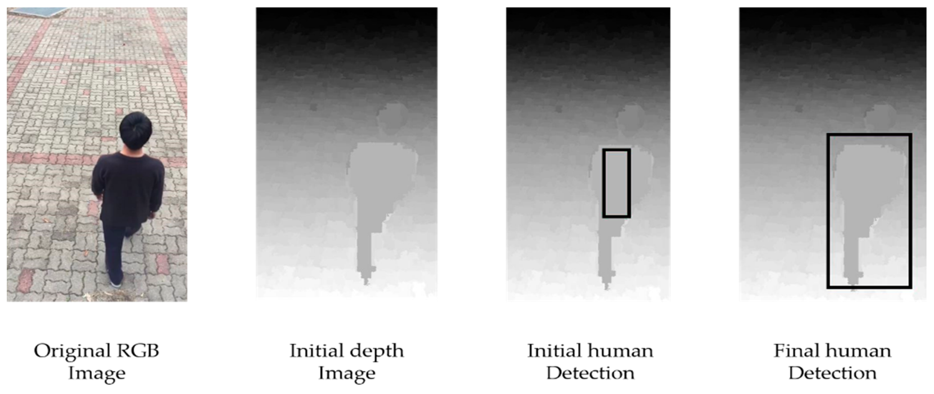
where $f(P_i)={\displaystyle {\sum }_{i=0}^w{\displaystyle {\sum }_{j=0}^h(I(x+i,y+j)-\overline{I})}}$ and $P_i=\{w,h,x,y\}$. The function $f(P_i)$ is the objective function to be minimized to find the optimum size $\left(w,h\right)$ and location of the local window $\left(x,y\right)$ enclosing a human body shape. The symbols, $w,h,x,y$, indicate the window width, window height, and the $x$ and $y$ coordinates of the center of the window, respectively. $I_w,I_h$ and $L_w,L_h$ denote the image width and height and the window width and height, respectively. $I(x,y)$ is the intensity value at $(x,y)$ and $\overline{I}$ is the mean of all pixels in the local window. Figure 4 shows the human detection process using the PSO method. In the depth image, the region having the smallest variance is found and the depth information in the region is used to expand the region. In this way, the final (red) rectangular box is detected and the inside (foreground) and the outside (background) information are separated from each other and used for the graph-cuts method.

2.3. Rao-Blackwellized Particle Filter-Based Human Tracking

2.3.1. Rao-Blackwellized Particle Filter (RBPF)

Kalman filter and Extended Kalman filter are two representative estimation methods used for object tracking using the Bayesian filtering method. They work on linear state space models and non-linear state space models, respectively, and many estimation problems are solved using these two filtering methods. However, these methods assume the Gaussian approximation, which may not work in certain real-world scenarios. A sequential importance resampling algorithm is proposed to solve the non-linearity and non-Gaussian problems. This algorithm first represents the posterior distribution of the state vector using particles with weight factors. The resampling step then removes the low-weight particles and duplicates the high-weight particles to reduce the variance [37]. The set of particles is then reweighted and updated recursively. The Sequential Importance Resampling (SIR) algorithm [38] produces the following filtering distribution. Equation (5) represents the filtering for a weighted set of particles $\left\{\right(w_k^{\left(i\right)},x_k^{\left(i\right)}):i=1\cdots N\}$.

$$p(x_k|y_{1:k})\approx {\displaystyle \sum _{i=1}^N{\omega }_k^{(i)}\delta (}{x}_k-x_k^{(i)})$$

(5)

Rao-Blackwellization refers to a kind of marginalization in which the parts that can be evaluated analytically in the filtering equation are separately calculated and the remaining parts are calculated using the Monte Carlo sampling method [39]. Thus, Equation (5) is divided into two parts, as shown in Equation (6).

$$p(u_{0:k},x_{0:k}|y_{1:k})=p(x_{0:k}|u_{0:k},y_{1:k})p(u_{0:k}|y_{1:k})$$

(6)

where $x_k$ is the state, $y_k$ is the measurement, and $u_k$ is an arbitrary latent variable. Here, the first term is analytically solved using a Kalman filter or an extended Kalman filter and the second term is solved using the Monte Carlo sampling method.

$$\begin{array}{l}p(u_{0:k}|y_{1:k})\propto p(y_k|u_{0:k},y_{1:k-1})p(u_{0:k}|y_{1:k-1})\\ =p(y_k|u_{0:k},y_{1:k-1})p(u_k|u_{k-1})p(u_{0:k-1}|y_{1:k-1})\end{array}$$

(7)

where we have used the Markovian property $u_k$. Importance distribution can be used to obtain the following weight recursion:

$${\omega }_k^{(i)}\propto \frac{p(y_k|u_{0:k-1}^{(i)},y_{1:k-1})p(u_k^{(i)}|u_{k-1}^{(i)})}{\pi (u_k^{(i)}|u_{0:k-1}^{(i)},y_{1:k})}{\omega }_{k-1}^{(i)}$$

(8)

This is a mathematical formulation of RBPF [40].

2.3.2. RBPF-Based Human Tracking

Our aim is to model the shape of a person as an ellipse and to estimate the state recursively using a state vector and an observation vector. The state vector and observation vector are defined as follows:

$$x_t={(x_c,y_c,a,b,v_x,v_y,\theta )}^T$$

(9)

where $\left(x_c,y_c\right)$ is the human position, $\left(a,b\right)$ are half lengths of the major and minor axis of the ellipse, $\left(v_x,v_y\right)$ is the velocity in 2D Cartesian coordinates, and θ is the angle of measure of the ellipse’s rotation with respect to the image x-axis. The points on the human contour from the binary image obtained from the detection step are defined as an observation vector: $y_k=\left\{x_i,y_i\right\},i=1\cdots p$ where, $k$ is the time step, $p$ is the number of points on the contour, and $x_i,y_i$ are the $x$ and $y$ coordinates of each point. In this study, an observation vector is defined as follows using 10 points:

$$y_k={\{y_1^T,y_2^T,y_3^T,y_4^T,y_5^T,y_6^T,y_7^T,y_8^T,y_9^T,y_{10}^T\}}^T$$

(10)

The non-linear function $h$ defines the general parametric ellipse equation given by:

$$h(x_t)=\left[\begin{array}{c}X(\theta )=x_c+a\cos (\theta )\cos (\phi )-b\sin (\theta )\sin (\phi )\\ Y(\theta )=y_c+a\cos (\theta )\sin (\phi )+b\sin (\theta )\cos (\phi )\end{array}\right]$$

(11)

where $\theta \in \left[0,2\pi \right]$ and φ are angles with respect to the x-axis. The Jacobian of $h$ is given by:

$$\begin{array}{l}H(x_t)=\left[\begin{array}{c}\frac{\partial X\left(\theta \right)}{\partial x_t}\\ \frac{\partial Y(\theta )}{\partial x_t}\end{array}\right]\\ =\left[\begin{array}{c}\begin{array}{ccc}\begin{array}{ccc}\begin{array}{cc}1& 0\end{array}& \cos (\theta )\cos (\phi )& -\sin (\theta )\sin (\phi )\end{array}& -a\cos (\theta )\sin (\phi )& -b\sin (\theta )\cos (\phi )\end{array}\\ \begin{array}{ccc}\begin{array}{cc}\begin{array}{cc}\begin{array}{cc}0& 1\end{array}& \cos (\theta )\sin (\phi )\end{array}& \sin (\theta )\cos (\phi )\end{array}& a\cos (\theta )\cos (\phi )& -b\sin (\theta )\sin (\phi )\end{array}\end{array}\right]\end{array}$$

(12)

The likelihood function of the observations approximate to Gaussian density as follows [41]:

$$p(y_t|x_t)\propto N(D_t;0,{\sigma }^2)=\frac{1}{\sqrt{2\pi {\sigma }^2}}exp\left\{-\frac{D_t^2}{2{\sigma }^2}\right\}$$

(13)

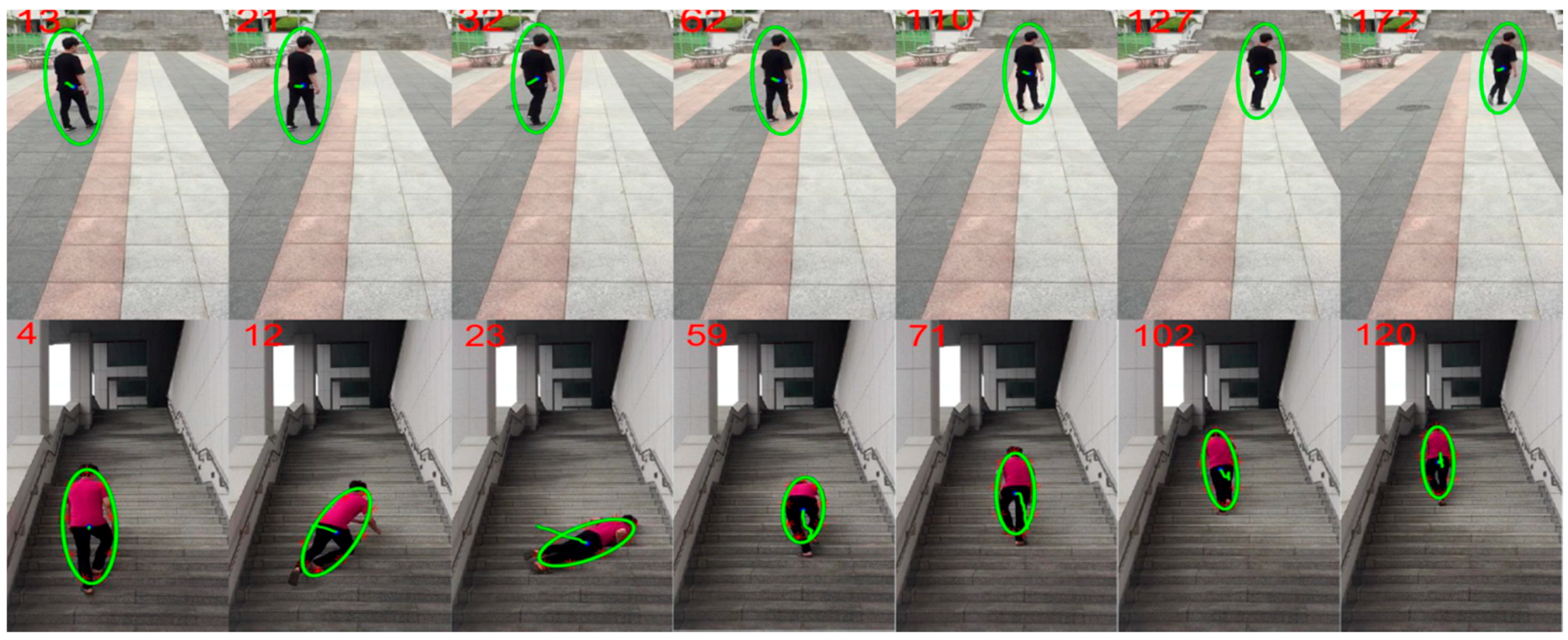
D_t is the Euclidean distance between the predicted observations of the target and true observations y_t obtained from the detection step, specified by the state vector x_t. The standard deviation σ of the Gaussian density [42] depends on the designer. Figure 5 represents the human tracking result based on the RBPF algorithm at different locations. The upper images show the normal case during which the subject does not fall throughout the duration of the scene and the lower images indicate the scenario in which the subject falls during the scene.

2.4. 3D Fall Detection

2.4.1. Feature Extraction

As described in the introduction, different features such as the ratio of minor axis to major axis, area, head position, shape orientation, and 3D movement have been used in many fall detection studies. Among the features, the vertical velocity is the most conspicuous feature when a fall is detected, and also after the fall occurs, the motionless time is monitored to detect an emergency situation [43]. In this study, we divide a fall event into five states and use adaptive features to distinguish falling postures, such as front falling, back falling, and side falling from confounding normal motions (squatting, sitting, and bending). We use three main features to classify the falling event into five states.

• Silhouette features: for the ellipse model estimated by human tracking, features (orientation, positions of major and minor axes) are extracted from the silhouette of a human.
• Depth features: depth values at the two distinct end points of the major axis of the ellipse model. The depth values are generated by a supervised learning method [32,33,34].
• Velocity features: vertical velocity shows how the height difference changed during a certain period. The velocity is calculated by measuring the height difference (Euclidean distance) between the top and bottom positions in a predefined time period (e.g., 5 frames in our study providing a clear cue of the potential fall). In addition to this, we also use the gradient of the top and the center positions to make a judgment of the no-motion phase.

2.4.2. Features-Based Fall State Classification

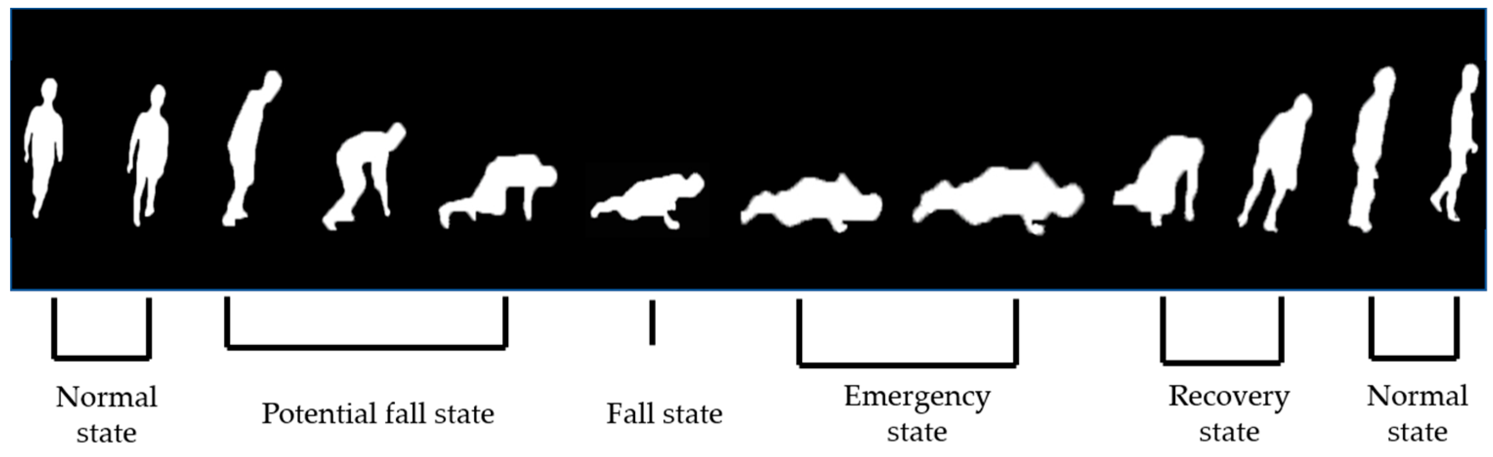
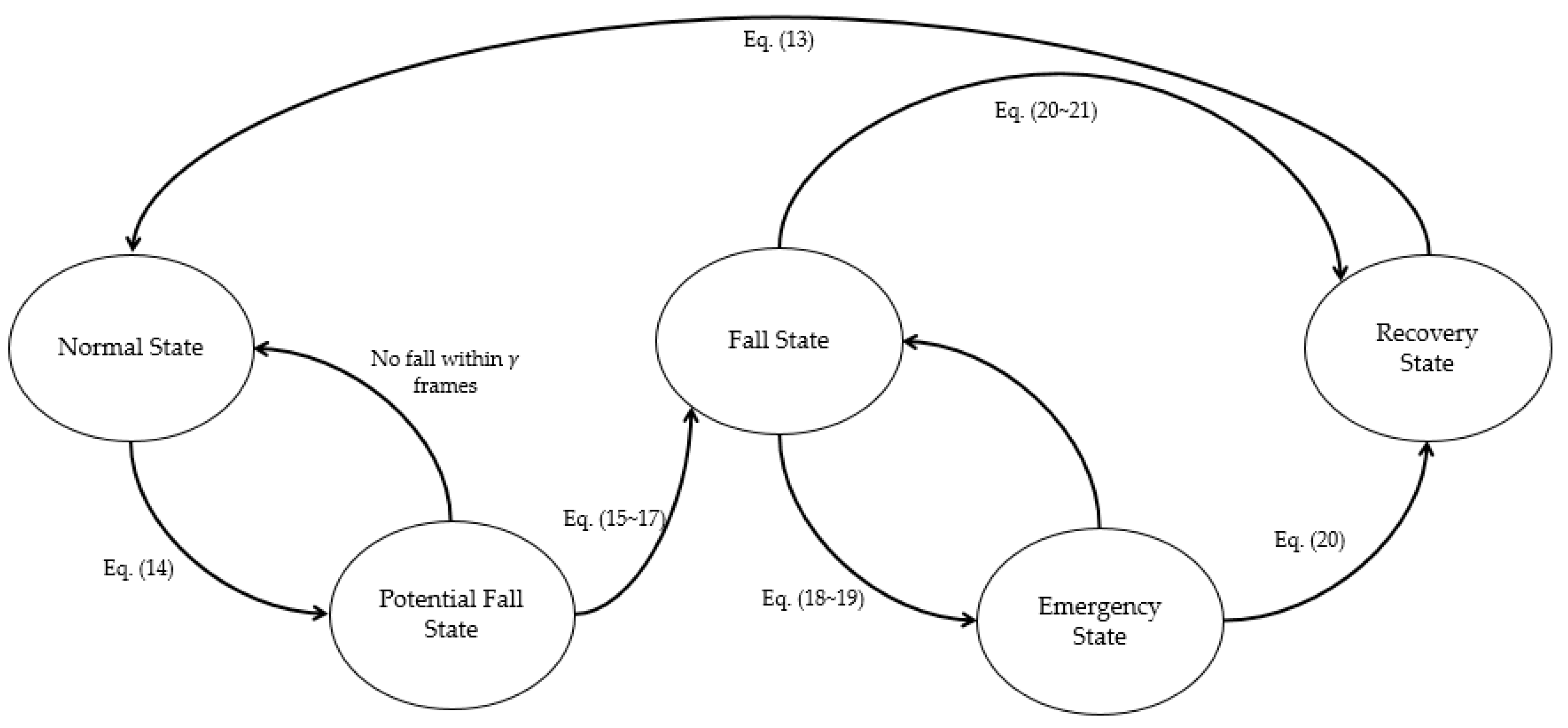
According to [2], a fall event is divided into four states: potential fall state, fall state, no-motion phase, and normal state. In this study, we define an additional recovery state that comes before returning to normal state after the emergency or fall state, so that the ending time of the emergency state can be informed more quickly. We use adaptive features to accurately classify the current state as seen in Figure 6. In the following, each state is described with necessary conditions to state transition illustrated in Figure 15.

• Normal state: If the ratio of the height difference in the current frame $h_d\left(c_k\right)$ to the height difference in the normal state $h_d(n_k)$ is larger than the value defined in Equation (14), it is judged to be the normal state again.

  $$\{\begin{array}{l}{\tilde{h}}_d=\frac{h_d(c_k)}{h_d(n_k)}>m\ast \theta +n,0\le \widetilde{h_d}\le 1\\ (m,n)=argmin\Vert \widehat{L}(\theta )-L_{fall}(\theta )\Vert \end{array}$$

  (14)
• Potential fall state: The most important characteristic of this state is that a human loses balance and the associated vertical velocity increases sharply. In our study, the potential fall state is the state satisfying Equation (15) while tracking.

  $$v_v\ge {\delta }_1$$

  (15)

  where $v_v$ is the vertical velocity and ${\delta }_1$ is a predefined threshold. If it does not enter the fall state for a certain period, it returns to the normal state.
• Fall state: The fall state begins when the upper body of a person touches the ground and the height difference between the top and bottom positions of the major axis are significantly different from the normal state. From a technical point of view, 2D information is not enough to determine a fall. Hence, we define three conditions, (16), (17), (18), that use both 2D and 3D features to improve fall detection. To be considered as the fall state, all of the following conditions should be met:

  $$\{\begin{array}{l}{\tilde{h}}_d=\frac{h_d(c_k)-h_d(n_k)}{h_d(n_k)}>m\ast \theta +n,0\le \widetilde{h_d}\le 1\\ (m,n)=argmin\Vert \widehat{L}(\theta )-L_{fall}(\theta )\Vert \end{array}$$

  (16)

  $$\frac{b}{a}>{\delta }_2,0\le {\delta }_2\le 1$$

  (17)

  $$\left[\frac{d_t}{d_b}\right]=1$$

  (18)

  where $h_d(c_k)$ and $h_d(n_k)$ are the height difference between current frame $c_k$ and last frame $n_k$ of the normal state. $\theta$ is the slope of the major axis of the ellipse model and $m,n$ are the line parameters of $\widehat{L}(\theta )$ (line at $\theta$), estimated by the method of least squares with $L_{fall}(\theta )$ (precomputed line to a fall at $\theta$) that was pre-calculated by pilot experiments. $a$ and $b$ are the major and minor axes, respectively. The notations $d_t,d_b$ are the depth values at the top and the bottom positions, respectively and ${\delta }_2$ is the predefined threshold. If any of the conditions are not satisfied, either temporarily or permanently, it returns to the normal state.
• No-motion phase: This phase is a condition that indicates the motionless period of the human after the fall state. To detect motion change in this phase, we use two gradient features, namely $\nabla p_t(c_k)$ and $\nabla p_c(c_k)$, they are the gradients at the top and center position. If these two gradient values satisfy Equation (19), it is initially classified as no-motion and if this condition is continuously satisfied over a period of $\tau$ frames, the fall state is judged as an emergency state.

  $$\{\begin{array}{l}\nabla p_t(c_k)<{\delta }_3\\ \nabla p_c(c_k)<{\delta }_4\end{array}$$

  (19)

  $$t_{nomotion}>\tau$$

  (20)

  where $\tau$ is the threshold value that can be set arbitrarily according to the desired time. If the two gradient values are greater than threshold values ${\delta }_3$ and ${\delta }_4$, the fall state changes to the next state which is the recovery state.
• Recovery state: This is in complete contrast to the fall state and represents the state when the upper body of a person rises from the ground and thus, the difference between the top or bottom from the current frame $c_k$ to the frame $n{m}_k$ in no-motion phase or $f_k$ in fall state is the most significant feature. If the previous state is the emergency phase, then, the state converts to a recovery state if Equation (21) is satisfied. If the previous state is the fall state and the interval between the current frame and the fall state start frame is greater than or equal to t, then the state changes from the fall state to the recovery state under Equation (21).

  $$\{\begin{array}{l}|p_t(c_k)-p_t(n{m}_k)|>{\delta }_5\\ |p_b(c_k)-p_b(n{m}_k)|>{\delta }_5\end{array}$$

  (21)

  $$c_k-f_k>\tau$$

  (22)
  Here, ${\delta }_5$ is our predefined threshold. With either condition satisfied, the body enters the recovery state from the previous state. All the states explained in the preceding sections are illustrated in Figure 7.

3. Experimental Results and Discussion

This section evaluates the performance of the proposed algorithm. For indoor fall research, testing datasets are publicly available; however, it is difficult to find testing datasets for outdoor falls because very little research has been done until now. We therefore recorded 38 testing video clips, consisting of 4271 frames in total, at three different locations including both indoor and outdoor environments with six people to evaluate our fall detection method. With the datasets, the performance in terms of sensitivity, specificity, accuracy, and error was measured for a quantitative evaluation. The frame rate of our testing dataset is 12 fps and the resolution of the images is 720 × 404 pixels. Video recording was performed using a simple smart phone camera (iPhone 5s) and multiple camera angles were used. A total of 27 fall scenes depict the falling postures, such as falling front, back, side (right and left), and other motions based on the orientation of the fall. Eleven confounding scenes include sitting, squatting, and bending, which are the motions that make it difficult to distinguish between a fall and normal motion. Prior to the main experiments, we conducted pilot experiments to find the optimum values of thresholds used for our algorithm with 24 separate datasets. We used the Matlab 2017 version to simulate the fall detection algorithm.

3.1. State Analysis

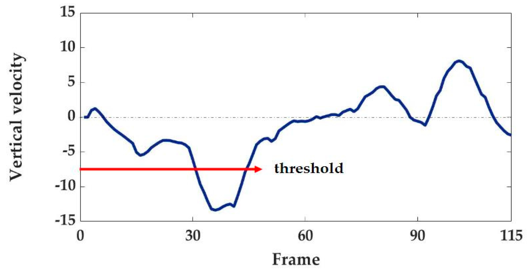
First, we use the threshold value as the vertical velocity to detect the start point of the potential fall period. The threshold value is the same for all scenes. This means that the pixel difference between the top and bottom positions must be more than the predefined value, within the period spanning 12 frames, to begin the potential fall state. Figure 8 shows the vertical velocity feature used to detect a potential fall state. When the vertical velocity meets a predefined threshold, the normal state becomes a potential fall state. The end frame of the normal state is identified by detecting the start frame of the potential fall state. The start frame of the fall state can be detected by measuring the change in the height difference of the ellipse model.

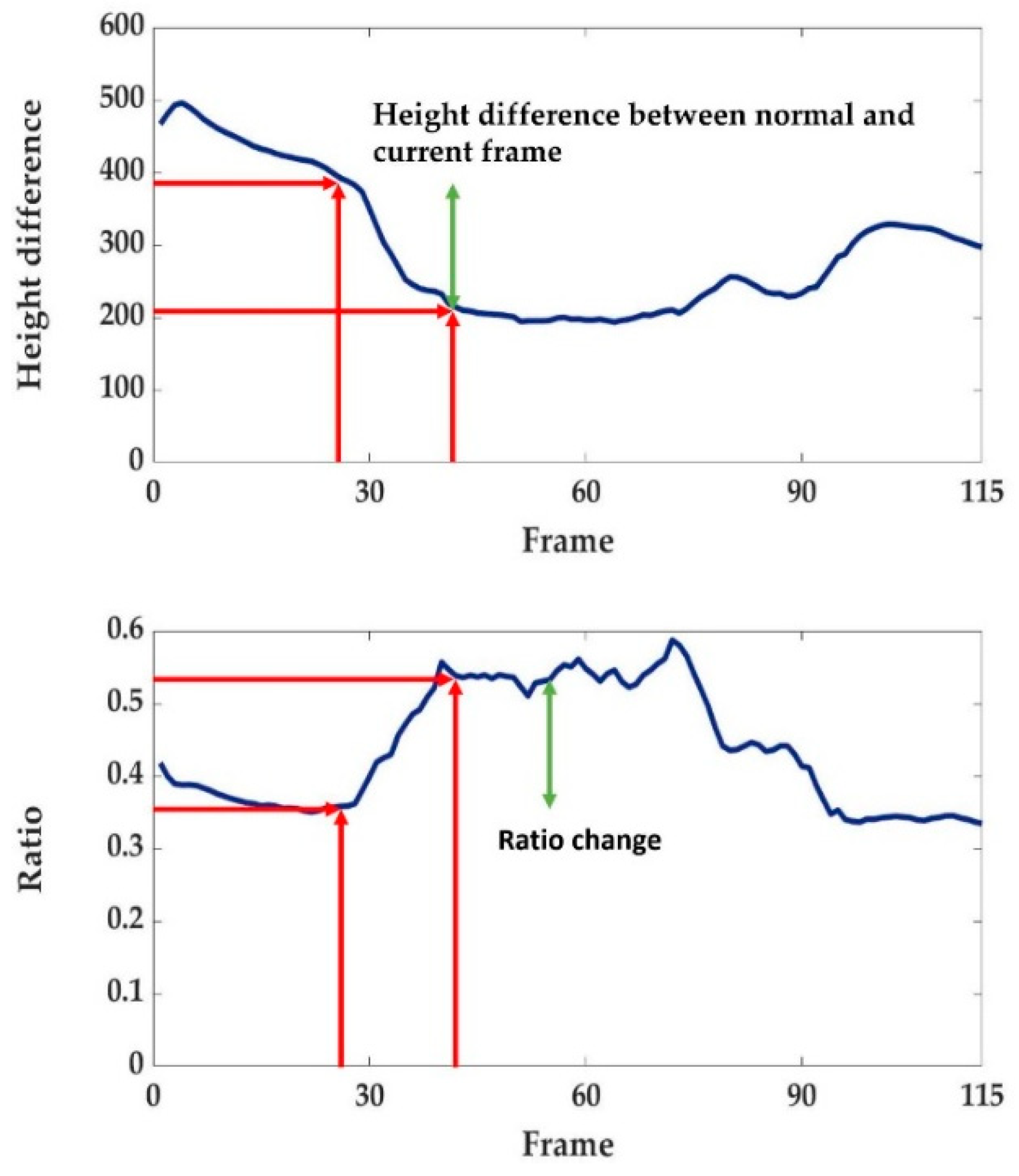
The plots of Figure 9 are an example of successful detection of the fall state near the 45th frame. Note that the vertical axes of the two plots in Figure 9 are the height difference of the major axis of the ellipse model and the ratio of minor axis to major axis, respectively. The ratio of minor axis to major axis feature is also used to account for the changes in the length of the major axis due to the motions, such as bending, squatting, and sitting. In the case of bending, the length of the upper body reduces and, in the case of squatting, the length of the lower body reduces, consequently changing the length of the major axis when confounding motion occurs. However, in case of a general fall, the ratio of major axis to minor axis is almost always maintained. Therefore, we use these two features to detect the fall start point accurately. The no-motion phase is defined as no movement after the fall state. Therefore, in this state, the gradient values at the top and the bottom positions must be below the predefined threshold. Figure 10 shows an example where the gradient is lower than the threshold (see the red arrow between the 30th and the 50th frames). At the end of the no-motion phase, the most noticeable feature is the movement of a human’s head or leg.

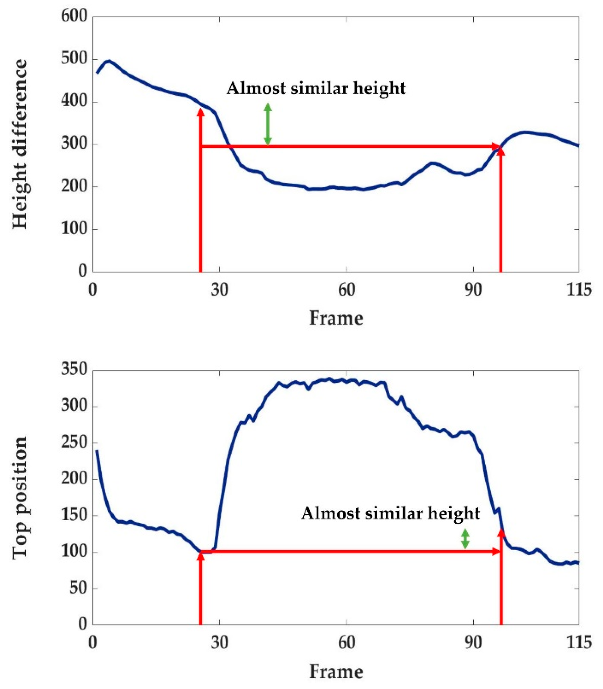
In this study, the recovery state begins when the upper body is completely off the floor, which is the case of the change in the top position above the predefined threshold. However, in the case of a back fall, the position of the head is opposite to that in case of a front fall, so the change rate of the top position and bottom position is observed differently depending on the slope of the fall. As shown in Figure 11, the recovery state begins when the difference exceeds the threshold of the red arrow. If the height difference in the current frame is closer to the height difference in the normal state, the recovery state is changed to the normal state. The criterion used here is adaptively determined using the same value that was used to determine the fall. Every state and feature is described in Figure 12. For the evaluation experiments, we use optimized values for all of the thresholds (${\delta }_1=7$, ${\delta }_2=0.25$, ${\delta }_3=6$, ${\delta }_4=4.5$, ${\delta }_5=26$) gathered by pilot experiments. Velocity threshold ${\delta }_1$ refers to the commonly reported fall velocity. Moreover, ${\delta }_2$ is the ratio of the minor axis to the major axis, which indicates how much the shape of a person changes. Symbols ${\delta }_3$ and ${\delta }_4$ represent the threshold for the top and bottom position gradient of the ellipse. These are the values that physically represent the movement of a person’s head or leg in a gradient. ${\delta }_5$ refers to the transition threshold from the no-motion phase to the recovery state, which indicates that there is a difference in head or leg height during the recovery.

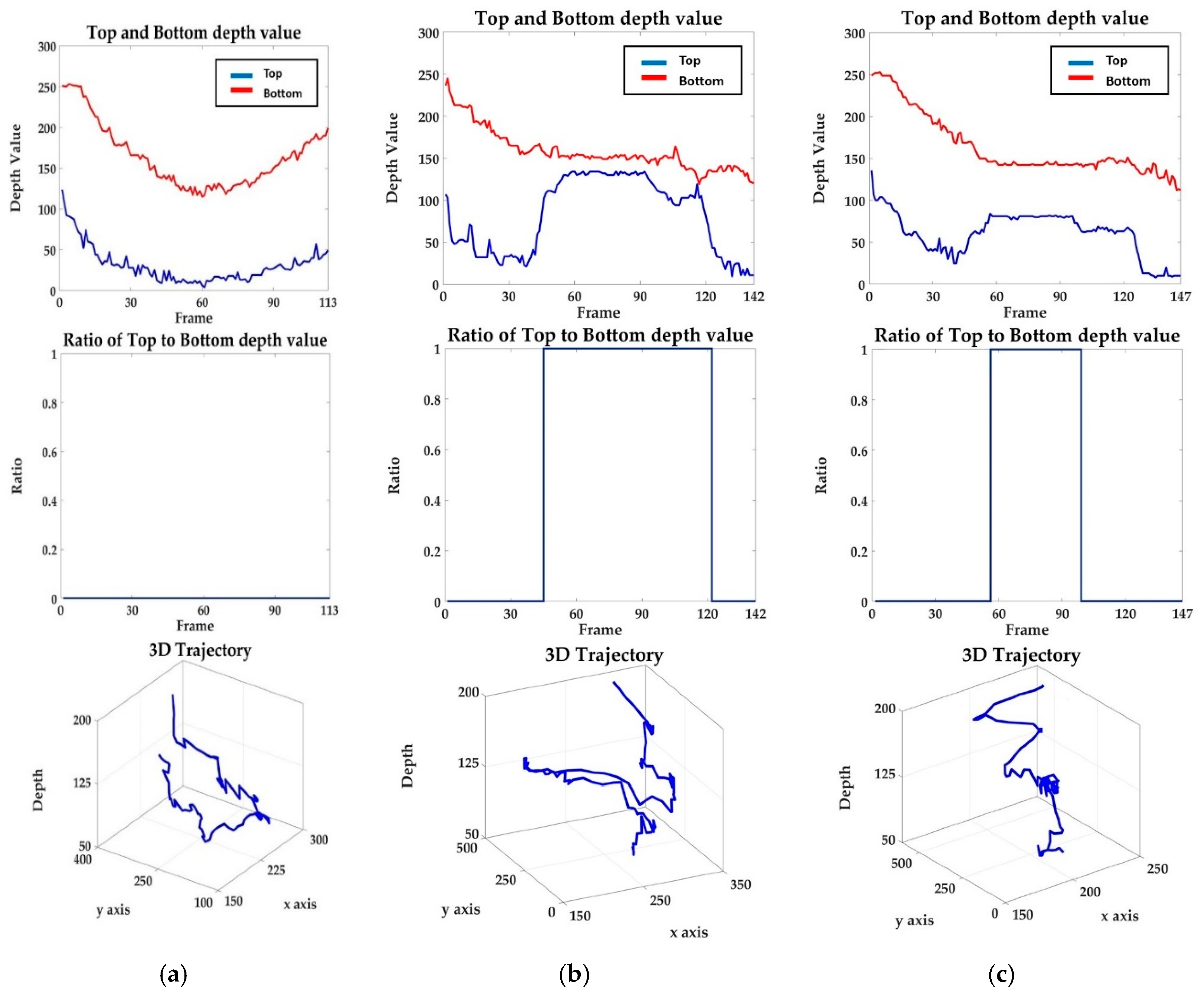
Figure 13 shows the depth values (top line) and the ratio (middle line) of the top and bottom positions of the individual along with the 3D trajectory (bottom line) for the three cases. Figure 13a represents the normal walking scenario, in which the subject is gradually moving away and coming back again. Figure 13b demonstrates the scenario involving the side fall and Figure 13c represents the scenario in which the subject falls in the camera view direction. Here, we use a depth image of the background. This method differs from background modeling that is vulnerable to background changes. However, this method does not need to update the background scene constantly because it only needs just one depth map of a single background image including a CCTV wide angle. Moreover, it does not need to use different background images over time. The human’s top and bottom positions, obtained through human tracking, are assigned to the depth map of the background to extract the depth value for those positions, which are then depicted by the graphs on the upper line in Figure 13. In a walking scene, where a person moves away from the camera and close to the camera, the corresponding depth values become smaller and larger, respectively. Moreover, in case of front/back and side falling, the bottom position is almost the same. The difference between the bottom and top position becomes larger in front or back falling cases. The depth values are depicted by the upper line of the graph represented in Figure 13. The middle line of the graph is calculated by rounding off the ratio of the depth values of the top to bottom positions. The state recorded as 1 is almost the same as that of the actual fall and no-motion phase, which shows that reliable information can be obtained from the 3D feature. The bottom line graphs represent 3D trajectories for human tracking. In the walking scene the depth value changes naturally, and in the scenes containing the fall there are unique sections in the depth value. Therefore, fall detection can be improved by additionally using the depth information.

Table 1. 3D mean error obtained from walking (Case 1), side fall (Case 2), front/back fall (Case 3).

Case 1	Error Rate (%)	Case 2	Error Rate (%)	Case 3	Error Rate (%)
Frame 1	12.6	Frame 1	5.6	Frame 1	8.9
Frame 13	6.9	Frame 13	16.5	Frame 13	0.1
Frame 25	12.1	Frame 25	12.5	Frame 25	18.2
Frame 37	3.8	Frame 37	3.1	Frame 37	11.6
Frame 49	2.1	Frame 49	3.9	Frame 49	5.3
Frame 61	10.5	Frame 61	3.1	Frame 61	6
Frame 73	7.6	Frame 73	4.4	Frame 73	6
Frame 85	5.4	Frame 85	4.4	Frame 85	5.8
Frame 97	10.3	Frame 97	4.4	Frame 97	5.8
Frame 109	18.4	Frame 109	6.3	Frame 109	5
Average	8.97	Average	6.42	Average	7.27

lists the 3D mean error of scenes that include walking, side fall, front fall, and back fall. The error is the difference between a 3D value estimated by our tracking algorithm and a real 3D value measured with a ruler. This was possible since we found that there is a linear relationship between the physical and estimated distance with a depth map generated from a single RGB image. More specifically, the human’s bottom position is estimated through human tracking and the corresponding depth value is obtained using the depth map, which is derived through the background image as described in the preceding section. The real distance value is calculated through the depth versus real distance graph. Calculating the error between algorithm output and the real value yields the error rate shown in Table 1, which shows that our algorithm can provide reliable real distance values from a single camera. The error interval is approximately 12 frames because we acquire 12 frames per second.

Figure 14a shows the result of state classification based on the features obtained earlier, which is similar to [44] in terms of fall severity levels from the normal to the emergency. The overall fall process is divided into five states and, as mentioned previously, the prior state requirements have to be met for moving onto the next state. When a person’s vertical velocity changes suddenly, the indicator of the potential fall is turned on and the normal indicator is turned off. From this moment, the algorithm observes whether the condition for going to the fall state is satisfied or not. If a fall does not occur for a certain period, the normal indicator is turned on. If the fall indicator is turned on, we need to observe if the fall is temporary or permanent. If there is no human motion for a prolonged period, the no-motion indicator is turned on. The duration of the no-motion phase is monitored to raise the emergency signal and the criteria for this duration may vary. When no incident of fall is detected, the state from fall to recovery must remain zero. Figure 14b,c show the normal and fall indicators when confounding motion occurs, such as sitting and squatting motion respectively. If the potential fall indicator is not turned on, both the no-motion indicator and the recovery indicator are not turned on. The proposed algorithm accurately judges these confounding motions as normal motion. Figure 15 shows the state transition diagram for the fall detection process proposed in this paper. It shows how the change among normal state, potential fall state, fall state, emergency state, and recovery state occurs under certain conditions.

3.2. Evaluation of Fall Detection

The criteria for evaluation of our method utilizes well-known metrics in the fall detection study [45].

$$\begin{array}{l}Sensitivity=\frac{TP}{TP+FN}\\ Specificity=\frac{TN}{TN+FP}\\ Accuracy=\frac{TN+TP}{TN+TP+FN+FP}\\ Error=\frac{FP+FN}{TP+TN+FP+FN}\end{array}$$

(23)

• True Positive (TP): A fall occurs, the device detects it.
• False Positive (FP): The device announces a fall, but it did not occur.
• True Negative (TN): A normal movement is performed, the device does not declare a fall.
• False Negative (FN): A fall occurs but the device does not detect it.

3.2.1. Fall Detection on Representative Scenes

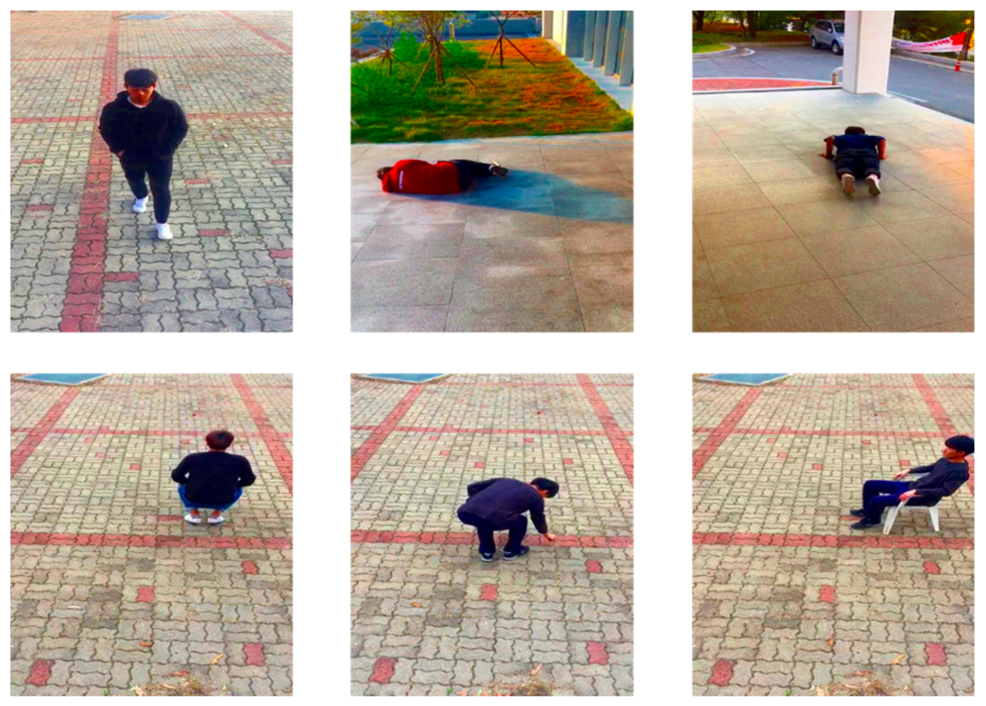
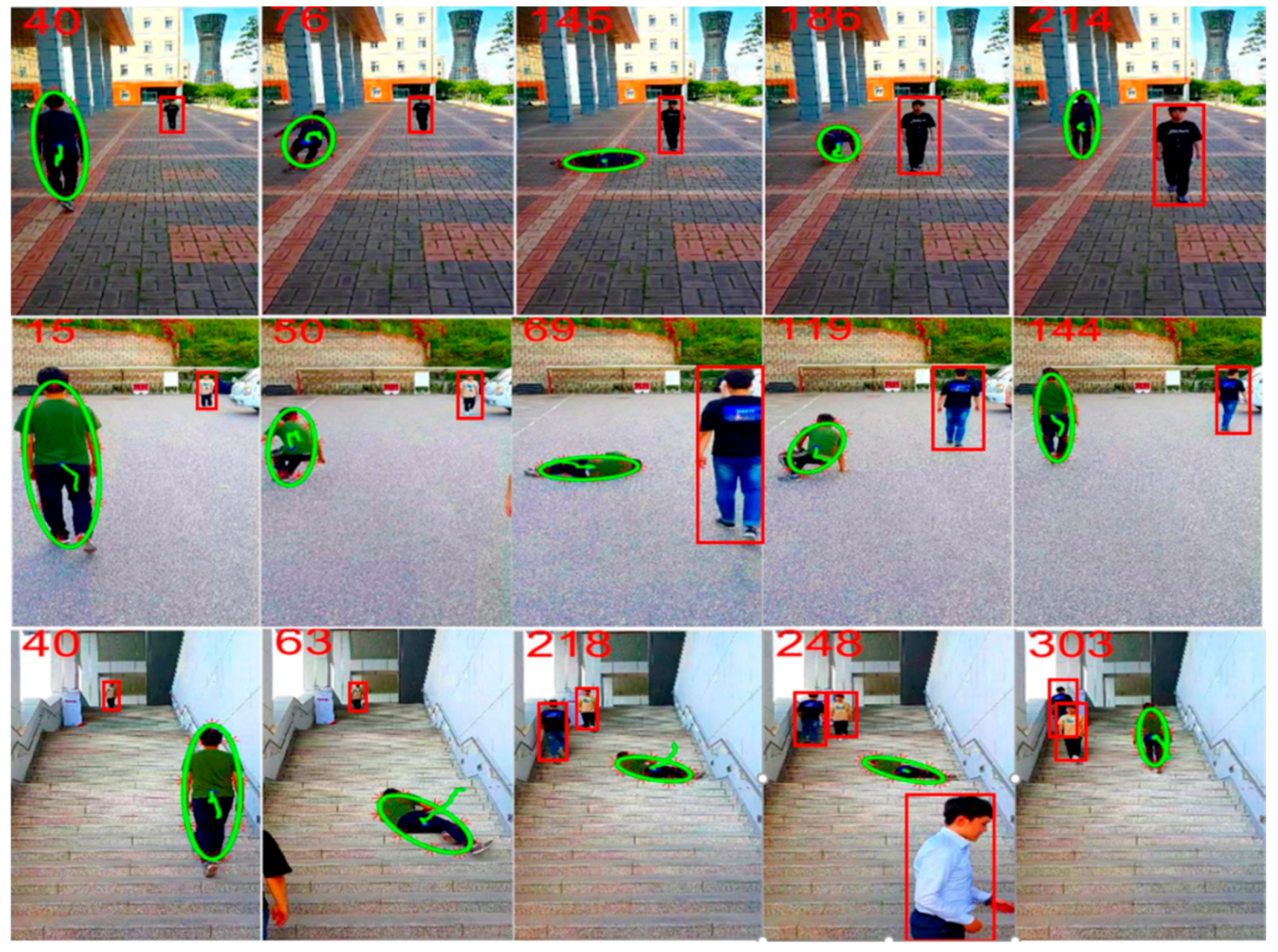
Figure 16 shows some representative scenes of datasets used in the evaluation experiment. The first three images in Figure 16 show a normal walking, side fall, and front fall scene from the left. The next three images are a squatting, bending, and sitting scene from the left. Experimental results evaluated with the metric (23) are summarized in

Table 2. Classification result of our system for representative scenes.

Person	Case	Our System	Ground Truth	Sensitivity (%)	Specificity (%)	Accuracy (%)	Error (%)
A	Bending	No alarm	No alarm	97.3% (Avg.)	99.5% (Avg.)	99.1% (Avg.)	0.9% (Avg.)
B	Side fall	52–96	52–95
	Front/back fall	54–100	55–98
C	Side fall	52–110	49–109
	Sitting	No alarm	No alarm
	Bending	No alarm	No alarm
	Squatting	No alarm	No alarm
D	Sitting	No alarm	No alarm
	Side fall	38–71	36–70
	Walking	No alarm	No alarm
	Bending	No alarm	No alarm
	Squatting	No alarm	No alarm

with respect to the sensitivity, specificity, accuracy, and the error rate of the representative scenes in Figure 16. Ground Truth in Table 2 indicates the manually recorded frames to test whether it detects falls accurately or not. The term ‘No alarm’ means that the fall indicator is not turned on. The sensitivity and specificity rate obtained from the experiment are similar or higher than those obtained in other studies for indoor fall detection. We cannot directly compare our results with others since our study focuses on an outdoor environment. However, these results (overall 99.1% success and 0.9% error) demonstrate that our algorithm is a promising approach for fall detection in an outdoor environment. Moreover, Figure 17 shows the tracking results for each case presented in Figure 16. Our algorithm can successively track all the cases from top to bottom.

3.2.2. Fall Detection in Various Fall Scenes

To verify our method more quantitatively, we tested all the datasets (38 videos consisting of 4271 frames in total) including confounding scenes and several normal walking, sitting, and standing scenes that might increase errors.

Table 3. Classification result of our system for all experiments.

TP	TN	FP	FN	Sensitivity (%)	Specificity (%)	Accuracy (%)	Error (%)
977	2106	27	44	95.7%	98.7%	97.7%	2.3%

represents the numerical results of the experiments. It is observed that the accuracy is slightly lower than the results presented in Table 2, which is sufficiently outstanding to detect various fall postures on the street. Additionally, we performed an experiment with the appearance of several people in one scene to measure the robustness of the fall detection algorithm, and the results showed successful fall detection of a single target person in the presence of multiple other people (two to four) without losing tracking as shown in Figure 18.

3.3. Robustness to Illumination Variations

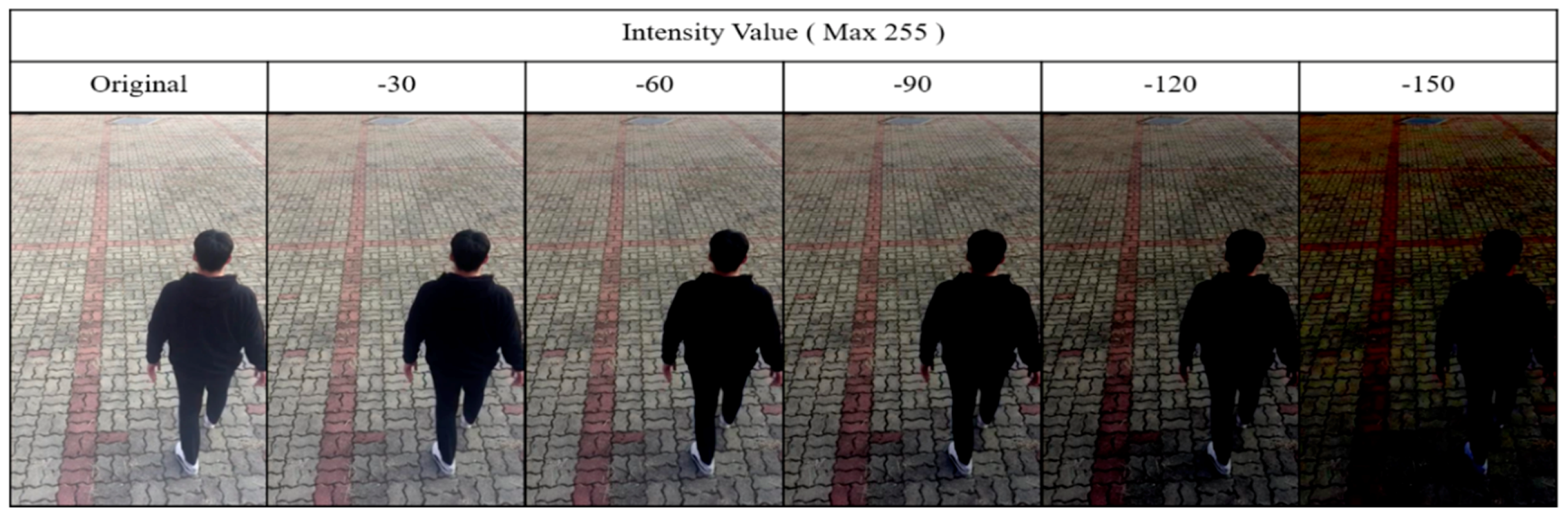
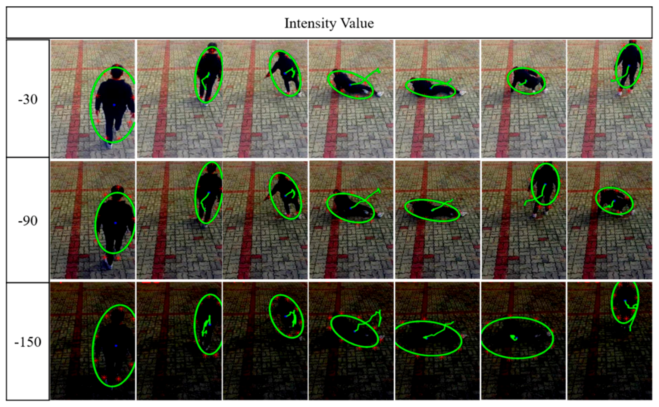
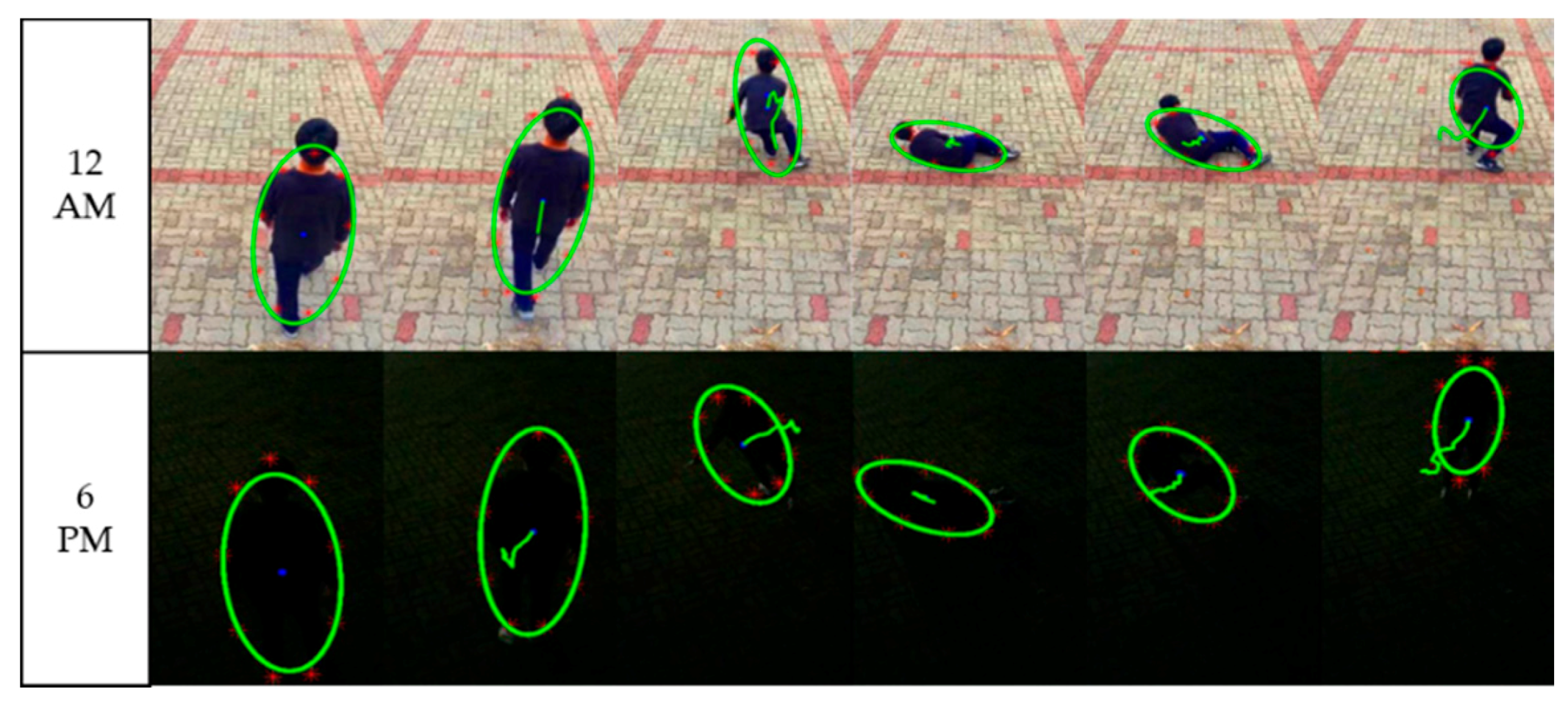
This study focuses on fall detection in an outdoor environment using equipment such as CCTV cameras. Therefore, the tracking algorithm needs to be robust against illumination changes in an outdoor environment to ensure optimum performance of the algorithm. Therefore, we tested our method by artificially controlling the intensity values of images of testing datasets to simulate illumination changes and then evaluated the accuracy of the tracking. Figure 19 shows a set of testing images simulating illumination changes from −30 pixel (slightly darker) to −150 pixel (darkest). In Figure 20, each line shows the tracking results with the testing images for each scene, respectively. As seen in the images, our tracking algorithm can accurately track a human’s state in the darkest image.

Table 4. The success rate with respect to synthetic illumination change.

Case/Pixel	30	60	90	120	150	Success Rate
Tracking	Success	Success	Success	Success	Success	100%
Fall detection	Success	Success	Success	Success	Success	100%

presents the tracking success rate and fall detection success rate when experimenting with four illumination changes. As changes in artificial illumination cannot adequately represent illumination changes in real environments, we also conducted tracking experiments with illumination changes in real environments. Figure 21 shows the tracking results at 12 pm and 6 pm. Sunset time is 6 pm in Korea and it is darker than when artificially subtracting 150. However, in this case, the ellipses more accurately represent the human, which means that artificially subtracting intensity value causes more information loss in the image than the actual illumination change. Therefore, in real environments, this algorithm can track people more accurately. Hence, we can confirm that this algorithm works robustly with changes in illumination, which is an important variable for an outdoor environment. Moreover, it is expected that the proposed method will be able to utilize the fall detection algorithm successfully in outdoor environments, considering it is more difficult to track black clothes in a dark environment.

4. Conclusions and Future Work

In this study, we propose a new approach for fall detection in an outdoor environment. There are two main contributions that our study makes. First, we developed a new fall detection algorithm that works accurately, even with a single camera, in an outdoor environment. Second, our method shows a new approach that combines 2D and 3D features of a depth image generated by a supervised learning method from a single RGB image to significantly improve fall detection in an outdoor environment. Our approach is a promising development, because we can use 3D information without using a special camera, such as the Kinect sensor, a depth sensor, or a multiple camera system. In addition, our method performs human detection using the particle swarm optimization method to locate the area of minimum variance on the aforementioned depth image. Consequently, this method solves the initialization problem mainly encountered in previous tracking studies.

Furthermore, it can be said that the rapid changes in the background and considerable variation in illumination of an outdoor environment makes it is difficult to use the depth camera to perform segmentation smoothly. However, in this study, we successfully performed fall detection studies in various outdoor environments due to the fact that we do not use the background reference image for segmentation; one of the only requirements of this study is a depth image taken with a normal RGB camera. Moreover, in this study we experimented with several illumination changes to establish the accuracy of the algorithm. Through various experiments, we showed that the proposed method robustly detects falls in complex environments and that the tracking algorithm used in this study works accurately even when the illumination changes, suggesting the possibility of using it in surveillance systems of outdoor environments. For future work, we plan to carry out fall detection research in an outdoor environment comprising of more than one person, multiple cars, and many other objects that are intricately intertwined. The final research goal is to construct a social safety net based on surveillance systems to detect multiple people and multiple falls that simultaneously occur within a single scene.

References

- Ageing, W.H.O.; Unit, L.C. WHO Global Report on Falls Prevention in Older Age; World Health Organization: Geneva, Switzerland, 2008. [Google Scholar]
- Feng, W.; Liu, R.; Zhu, M. Fall detection for elderly person care in a vision-based home surveillance environment using a monocular camera. Signal Image Video Process. 2014, 8, 1129–1138. [Google Scholar] [CrossRef]
- Shany, T.; Redmond, S.J.; Narayanan, M.R.; Lovell, N.H. Sensors-based wearable systems for monitoring of human movement and falls. IEEE Sens. J. 2012, 12, 658–670. [Google Scholar] [CrossRef]
- Zhao, G.; Mei, Z.; Liang, D.; Ivanov, K.; Guo, Y.; Wang, Y.; Wang, L. Exploration and implementation of a pre-impact fall recognition method based on an inertial body sensor network. Sensors 2012, 12, 15338–15355. [Google Scholar] [CrossRef] [PubMed]
- Kangas, M.; Konttila, A.; Lindgren, P.; Winblad, I.; Jämsä, T. Comparison of low-complexity fall detection algorithms for body attached accelerometers. Gait Posture 2008, 28, 285–291. [Google Scholar] [CrossRef] [PubMed]
- Nguyen, T.-T.; Cho, M.-C.; Lee, T.-S. Automatic fall detection using wearable biomedical signal measurement terminal. In Proceedings of the Annual International Conference of the IEEE Engineering in Medicine and Biology Society, EMBC 2009, Minneapolis, MN, USA, 3–6 September 2009; pp. 5203–5206. [Google Scholar]
- Bourke, A.K.; Lyons, G.M. A threshold-based fall-detection algorithm using a bi-axial gyroscope sensor. Med. Eng. Phys. 2008, 30, 84–90. [Google Scholar] [CrossRef] [PubMed]
- Ariani, A.; Redmond, S.J.; Chang, D.; Lovell, N.H. Simulated unobtrusive falls detection with multiple persons. IEEE Trans. Biomed. Eng. 2012, 59, 3185–3196. [Google Scholar] [CrossRef] [PubMed]
- Doukas, C.N.; Maglogiannis, I. Emergency fall incidents detection in assisted living environments utilizing motion, sound, and visual perceptual components. IEEE Trans. Inf. Technol. Biomed. 2011, 15, 277–289. [Google Scholar] [CrossRef] [PubMed]
- Alwan, M.; Rajendran, P.J.; Kell, S.; Mack, D.; Dalal, S.; Wolfe, M.; Felder, R. A smart and passive floor-vibration based fall detector for elderly. In Proceedings of the 2nd Information and Communication Technologies, ICTTA’06, Damascus, Syria, 24–28 April 2006; pp. 1003–1007. [Google Scholar]
- Yazar, A.; Çetin, A.E. Ambient assisted smart home design using vibration and PIR sensors. In Proceedings of the 21st Signal Processing and Communications Applications Conference (SIU), Haspolat, Turkey, 24–26 April 2013; pp. 1–4. [Google Scholar]
- Yazar, A.; Keskin, F.; Töreyin, B.U.; Çetin, A.E. Fall detection using single-tree complex wavelet transform. Pattern Recognit. Lett. 2013, 34, 1945–1952. [Google Scholar] [CrossRef]
- Sixsmith, A.; Johnson, N.; Whatmore, R. Pyroelectric IR sensor arrays for fall detection in the older population. J. Phys. IV (Proc.) 2005, 128, 153–160. [Google Scholar] [CrossRef]
- Zigel, Y.; Litvak, D.; Gannot, I. A method for automatic fall detection of elderly people using floor vibrations and sound—Proof of concept on human mimicking doll falls. IEEE Trans. Biomed. Eng. 2009, 56, 2858–2867. [Google Scholar] [CrossRef] [PubMed]
- Rougier, C.; Meunier, J.; St-Arnaud, A.; Rousseau, J. Fall detection from human shape and motion history using video surveillance. In Proceedings of the 21st International Conference on Advanced Information Networking and Applications Workshops, AINAW’07, Niagara Falls, ON, Canada, 21–23 May 2007; pp. 875–880. [Google Scholar]
- Vishwakarma, V.; Mandal, C.; Sural, S. Automatic detection of human fall in video. Pattern Recognit. Mach. Intell. 2007, 4815, 616–623. [Google Scholar]
- Rougier, C.; Meunier, J.; St-Arnaud, A.; Rousseau, J. Robust video surveillance for fall detection based on human shape deformation. IEEE Trans. Circuits Syst. Video Technol. 2011, 21, 611–622. [Google Scholar] [CrossRef]
- Qian, H.; Mao, Y.; Xiang, W.; Wang, Z. Recognition of human activities using SVM multi-class classifier. Pattern Recognit. Lett. 2010, 31, 100–111. [Google Scholar] [CrossRef]
- Anderson, D.; Keller, J.M.; Skubic, M.; Chen, X.; He, Z. Recognizing falls from silhouettes. In Proceedings of the 28th Annual International Conference of the IEEE Engineering in Medicine and Biology Society, EMBS’06, New York, NY, USA, 30 August–3 September 2006; pp. 6388–6391. [Google Scholar]
- Rougier, C.; Meunier, J.; St-Arnaud, A.; Rousseau, J. 3D head tracking for fall detection using a single calibrated camera. Image Vis. Comput. 2013, 31, 246–254. [Google Scholar] [CrossRef]
- Anderson, D.; Luke, R.H.; Keller, J.M.; Skubic, M.; Rantz, M.; Aud, M. Linguistic summarization of video for fall detection using voxel person and fuzzy logic. Comput. Vis. Image Understand. 2009, 113, 80–89. [Google Scholar] [CrossRef] [PubMed] [Green Version]
- Auvinet, E.; Reveret, L.; St-Arnaud, A.; Rousseau, J.; Meunier, J. Fall detection using multiple cameras. In Proceedings of the 30th Annual International Conference of the IEEE Engineering in Medicine and Biology Society, EMBS 2008, Vancouver, BC, Canada, 20–25 August 2008; pp. 2554–2557. [Google Scholar]
- Mastorakis, G.; Makris, D. Fall detection system using Kinect’s infrared sensor. J. Real-Time Image Process. 2014, 9, 635–646. [Google Scholar] [CrossRef]
- Stone, E.E.; Skubic, M. Fall detection in homes of older adults using the Microsoft Kinect. IEEE J. Biomed. Health Inform. 2015, 19, 290–301. [Google Scholar] [CrossRef] [PubMed]
- Gasparrini, S.; Cippitelli, E.; Spinsante, S.; Gambi, E. A depth-based fall detection system using a Kinect® sensor. Sensors 2014, 14, 2756–2775. [Google Scholar] [CrossRef] [PubMed]
- Ma, X.; Wang, H.; Xue, B.; Zhou, M.; Ji, B.; Li, Y. Depth-based human fall detection via shape features and improved extreme learning machine. IEEE J. Biomed. Health Inform. 2014, 18, 1915–1922. [Google Scholar] [CrossRef] [PubMed]
- Ko, M.; Kim, S.; Lee, K.; Kim, M.; Kim, K. Single camera based 3D tracking for outdoor fall detection toward smart healthcare. In Proceedings of the 2017 2nd International Conference on Bio-Engineering for Smart Technologies (BioSMART), Paris, France, 30 August–1 September 2017; pp. 1–4. [Google Scholar]
- Busching, F.; Post, H.; Gietzelt, M.; Wolf, L. Fall detection on the road. In Proceedings of the 2013 IEEE 15th International Conference on e-Health Networking, Applications & Services (Healthcom), Lisbon, Portugal, 9–12 October 2013; pp. 439–443. [Google Scholar]
- Sim, S.; Jeon, H.; Chung, G.; Kim, S.; Kwon, S.; Lee, W.; Park, K. Fall detection algorithm for the elderly using acceleration sensors on the shoes. In Proceedings of the 2011 Annual International Conference of the IEEE Engineering in Medicine and Biology Society, EMBC, Boston, MA, USA, 30 August–3 September 2011; pp. 4935–4938. [Google Scholar]
- Doukas, C.; Maglogiannis, I. Advanced patient or elder fall detection based on movement and sound data. In Proceedings of the Second International Conference on Pervasive Computing Technologies for Healthcare, PervasiveHealth 2008, Tampere, Finland, 30 January–1 February 2008; pp. 103–107. [Google Scholar]
- Iqbal, Q.; Aggarwal, J.K. Retrieval by classification of images containing large manmade objects using perceptual grouping. Pattern Recognit. 2002, 35, 1463–1479. [Google Scholar] [CrossRef] [Green Version]
- Saxena, A.; Schulte, J.; Ng, A.Y. Depth Estimation Using Monocular and Stereo Cues.
- Saxena, A.; Chung, S.H.; Ng, A.Y. Learning depth from single monocular images. In Proceedings of the Advances in Neural Information Processing Systems, Vancouver, BC, Canada, 5–8 December 2005; pp. 1161–1168. [Google Scholar]
- Saxena, A.; Chung, S.H.; Ng, A.Y. 3-D depth reconstruction from a single still image. Int. J. Comput. Vis. 2008, 76, 53–69. [Google Scholar] [CrossRef]
- Kennedy, J. Particle swarm optimization. In Encyclopedia of Machine Learning; Springer: Berlin, Germany, 2011; pp. 760–766. [Google Scholar]
- Boykov, Y.; Funka-Lea, G. Graph cuts and efficient ND image segmentation. Int. J. Comput. Vis. 2006, 70, 109–131. [Google Scholar] [CrossRef]
- Kitagawa, G. Monte Carlo filter and smoother for non-Gaussian nonlinear state space models. J. Comput. Graph. Stat. 1996, 5, 1–25. [Google Scholar]
- Doucet, A.; Godsill, S.; Andrieu, C. On sequential Monte Carlo sampling methods for Bayesian filtering. Stat. Comput. 2000, 10, 197–208. [Google Scholar] [CrossRef]
- Särkkä, S. Bayesian Filtering and Smoothing; Cambridge University Press: Cambridge, UK, 2013; Volume 3. [Google Scholar]
- Doucet, A. Rao-Blackwellized particle filtering for dynamic Bayesian networks. In Proceedings of the Conference on Uncertainty in Artificial Intelligence, Stanford, CA, USA, 30 June–3 July 2000; pp. 176–183. [Google Scholar]
- Jaward, M.; Mihaylova, L.; Canagarajah, N.; Bull, D. Multiple object tracking using particle filters. In Proceedings of the 2006 IEEE Aerospace Conference, Big Sky, MT, USA, 4–11 March 2006; p. 8. [Google Scholar]
- Kay, S.M. Fundamentals of Statistical Signal Processing: Practical Algorithm Development; Pearson Education: New York, NY, USA, 2013; Volume 3. [Google Scholar]
- Mirmahboub, B.; Samavi, S.; Karimi, N.; Shirani, S. Automatic monocular system for human fall detection based on variations in silhouette area. IEEE Trans. Biomed. Eng. 2013, 60, 427–436. [Google Scholar] [CrossRef] [PubMed]
- Fortino, G.; Gravina, R. Fall-MobileGuard: A smart real-time fall detection system. In Proceedings of the 10th EAI International Conference on Body Area Networks, Sydney, NSW, Australia, 20–30 September 2015; pp. 44–50. [Google Scholar]
- Noury, N.; Fleury, A.; Rumeau, P.; Bourke, A.; Laighin, G.; Rialle, V.; Lundy, J. Fall detection-principles and methods. In Proceedings of the 29th Annual International Conference of the IEEE Engineering in Medicine and Biology Society, EMBS 2007, Lyon, France, 22–26 August 2007; pp. 1663–1666. [Google Scholar]
Figure 1.
Proposed fall detection algorithm.
Figure 2.
Absolute (the right-hand side) and relative depth features (the left-hand side) used for estimating scene global depth (see [32] for details).
Figure 3.
The extracted depth maps: (a) the person in the image is about 5 m away from the camera and (b) the person in the image is about 2 m away from the camera.
Figure 4.
Human body detection process using a generated depth image.
Figure 5.
The human tracking result based on RBPF algorithm.
Figure 6.
Adaptive features for accurate state classification.
Figure 7.
State classification during the fall process.
Figure 8.
Vertical velocity and the corresponding threshold used to detect the start of the potential fall state.
Figure 9.
The upper image represents the height difference between the top and bottom positions and the bottom image indicates the ratio of minor axis to major axis that can be used to detect the start of the fall state.
Figure 10.
Fall detection feature that is applied to detect no-motion phase.
Figure 11.
Fall detection feature applied to detect the recovery state.
Figure 12.
Fall detection features applied to detect the normal state.
Figure 13.
Top and Bottom depth values (upper line) and Ratio of Top to Bottom depth value (middle line) and 3D trajectories (bottom line): (a) normal walking; (b) sideway fall; (c) optical fall.
Figure 14.
(a) Overall indicators for fall case; (b) Normal and Fall Indicator for sitting motion; (c) Normal and Fall indicators for squatting motion. (b,c) indicate normal cases. When the normal indicator is ‘ON’ and the fall indicator is ‘OFF’, it is interpreted as the ‘Normal State’ in case of sitting and squatting motion.
Figure 15.
State transition model of the proposed fall detection algorithm.
Figure 16.
Representative scenes and fall cases used for the evaluation.
Figure 17.
Resulting images of human tracking for various confounding cases: green colored ellipses demonstrate successful tracking and the red numbers are the image frame number.
Figure 18.
Results of tracking and fall detection in the presence of multiple other people (two to four from the top) in a scene. A person in a green ellipse is a target for tracking and fall detection.
Figure 19.
Testing images synthetically generated by reducing the pixel intensity for illumination changes.
Figure 20.
Tracking results with the synthetic testing images for illumination changes.
Figure 21.
Human tracking results in real illumination variations from midday light (noon) to evening time (6 pm right after sunset) in Korea.